Preprint
Article

Data-Driven Sparse Sensor Placement Optimization on Wings for Flight-by-Feel: Bioinspired Approach and Application

Altmetrics

Downloads

95

Views

50

Comments

0

A peer-reviewed article of this preprint also exists.

Submitted:

03 September 2024

Posted:

03 September 2024

You are already at the latest version

Alerts
Abstract
This research explores the feasibility of a data-driven optimization algorithm for placing sparse arrays of artificial hair-cell airflow velocity sensors to enable agile and robust flight-by-feel control of unmanned aircraft. The Sparse Sensor Placement Optimization for Prediction (SSPOP) algorithm exploits the information-rich features of large flow datasets to find a near-optimal set of locations for flow sensors on a wing. The flow information from these sensors can be used to predict flight state parameters such as the angle of attack, mimicking the fly-by-feel control systems observed in nature. We evaluate the effectiveness of this approach for a blunt-edged 45∘ swept delta wing. Exploiting the information in the complex airflow patterns over this wing, the SSPOP algorithm selects a sensor location design point (DP) which reliably ranks within the top 1% of all possible DPs by root mean square error in angle of attack prediction. This performance was consistent across models of various artificial hair lengths, and one model with variable hair lengths. This bioinspired dimension-reducing method for sensor placement optimization exhibits reliability and flexibility benefits when compared with a conventional greedy search algorithm and gradient-based optimization using auto-differentiation. The successful application of SSPOP in complex 3D flows paves the way for experimental evaluation of data-driven sparse sensor placement optimization for artificial hair-cell airflow sensors and is a major step toward biomimetic flight-by-feel.
Keywords: 
Subject: Engineering  -   Aerospace Engineering

1. Introduction

Aircraft design, perhaps more so than any other modern science, has its roots firmly planted in bioinspiration. However, until very recently, practical and technological constraints limited the extent of biomimicry. Birds and bats have continuously morphing wings with seemingly infinite configurations [1,2,3,4,5,6,7]; aircraft have slots, flaps, and, more rarely, active sweep. Bats and insects have hundreds or thousands of sensory hairs by which they feel the airflow; aircraft have one to several pitot probes and static ports. Recent advancements in materials and actuators have made possible continuously variable camber, twist, and planform [8], which may bring technology closer to matching the performance of natural flyers [9,10] These developments in morphing wing and sensor technology, as well as concurrent advances in understanding of extant [11] and extinct [12] animal flight, may be ushering in a new era of dexterous, nimble aircraft whose control systems are lighter, more robust, faster, and more information-rich than those of conventional aircraft [13]. A bioinspired systems-based approach is needed [14]; conventional sensors and control systems may be unreliable or infeasible for these emerging aircraft shapes, actuators, and integrated control surfaces [15,16].
A bioinspired Flight-By-Feel (FBF) system may employ integrated arrays of any number of pressure, strain, and flow sensors to enable rapid and agile flight state estimation and response [17] . Flying animals provide the proof-of-concept that FBF control is feasible, though the intricacies of their flight control systems remain poorly understood [18]. What is clear, at least, is that biological sensors are tailored for environment and behavior [19] and are seamlessly integrated into the body and wings [20]. The challenge for aircraft designers, constrained by size, weight, and power (SWaP) budgets, is to determine where best to place a limited number of sensors to detect the most useful information from the airflow over a wing or aircraft body. Optimal sensor placement may allow a handful of sensors to capture as much information as a dense array of randomly placed sensors, doing the same job but with less lag in closed-loop control, lower SWaP central processors, and easier integration. Sensor placement optimization can also be coupled with actuator design or placement optimization to achieve a lightweight structure capable of stability and control [21].
The functions describing the airflow over a wing in dynamic conditions are highly complex, nonlinear, and discrete, which poses severe difficulties for conventional optimization approaches. Likewise, a brute-force search of the design space, while feasible for small models, is prohibitive or impossible for realistic sensor placement problems. In this paper, we report that the data-driven Sparse Sensor Placement Optimization for Prediction (SSPOP) algorithm, first introduced for 2D airfoils [22,23,24], is capable of reliably finding a top-one-percent Design Point (DP), or set of sensor locations, for any number of sensors on a 3D wing, as ranked by accuracy in predicting the angle of attack (AoA or α ) from airflow velocity magnitude data. The performance of the SSPOP DP is compared against the best possible DP where brute force search is possible, and against some conventional optimization approaches, some of which are also bioinspired [25].
The SSPOP algorithm used here is an adaptation of the Sparse Sensor Placement Optimization for Classification (SSPOC) algorithm developed by Brunton et al. [26] and later expanded for Reconstruction (SSPOR) by the same group [27,28,29]. These optimization algorithms all use data reduction techniques to reduce the dimensionality of high-order systems. Like artificial hair sensors, data reduction for sensing is bioinspired. Animals interact with high-dimensional physical systems via limited sensory information, a form of compressive sensing of big data [30,31], and process diverse stimuli with limited sensor types as multi-modal signals [32,33].
In the present research, the sensors in the modeled FBF system were based on bat-like artificial hair-cell flow sensors (AHS), which detect velocity magnitude from mechanical drag force on hair-like structures (See [34] for bat hair-cell morphology and function, and [35,36] for a bat-like AHS). Some models included variable-length hairs, since hair length has been shown to have a significant impact on sensitivity [37,38]. A recent survey by the authors describes and evaluates hair-type and similar flow sensors to synthesize sensor design, function, placement optimization, FBF control, and next-generation aircraft design into a cohesive bioinspired research paradigm [22].
Most of the work in distributed sensing for FBF has involved the tractable cases of 2-D airfoils and rectangular wings on conventional-style aircraft, and rarely consider optimal placement (for a recent example of a square array of AHS used for flap-morphing gust alleviation, see [39]). This leaves the realms of complex flows, unsteady aerodynamics, and vortical flow largely unexplored. The flow over highly-swept wings, such as in the delta wing model used here (see Figure 2 in Section 2.1) includes prominent leading edge vortex (LEV) features, a common flow-control and lift-generating phenomenon found in nature [40,41,42,43,44,45,46] and increasingly in aircraft [47]. Figure 1 compares a physical and computational visualizations of a flapping dragonfly and a delta wing fighter aircraft, showing that both exhibit significant vortical flow structures. Flight control for aircraft with persistent LEVs is highly challenging [48], making a delta wing a prime candidate for evaluating the effectiveness of sensor placement optimization for flight-by-feel.
This work represents the first application of a data-driven approach for optimal placement of flow sensors on 3D wings, and the first application using variable-length hairs. These results confirm the conclusion from previous 2D studies ([22,23]) that the SSPOP algorithm is flexible in scale and scope, with promising FBF implications for sensors of any type and aircraft of any size. The successful application of SSPOP to 3D wings is a step toward solving the "grand challenge problem" of generalized optimization with scalability, which may enable rapid advancements in a broad range of engineering and system designs [27,28,29].

2. Materials and Methods

This paper covers the application and evaluation of the SSPOP algorithm for flow sensor placement on a delta wing. The following subsections describe the wing model, the SSPOP algorithm, and the brute-force search approach for verification of the results.

2.1. Wing Model

The model was a NACA 4415 delta wing with 45 sweep and a root chord of 250 mm. The wing geometry was constructed in Ansys DesignModeler as a half-span wing in a tunnel setting. Ansys Workbench and Ansys Fluent were used to perform computational fluid dynamics (CFD) modeling to acquire velocity data over a wide range of α . Ansys Fluent was used for grid generation of a polyhedral volume mesh limited to approximately 500 thousand cells for efficiency. Turbulent steady-state estimations of the flow field at 10 m/s freestream velocity were solved for each α from -10 to 20 at half-degree increments using constant density gas at standard conditions with a two-equation k- ω Shear-Stress Transport model. Each case was solved using a pseudo-transient pressure-based solver where the momentum equation and pressure-based continuity equations are solved simultaneously. This procedure was was validated by modeling a similar wing matching the geometry and conditions of an experimental wind tunnel test from [51], finding errors of approximately 2 % for the coefficients of lift ( c l ) and drag ( c d ) and 0.20 % for lift-to-drag ratio [23].
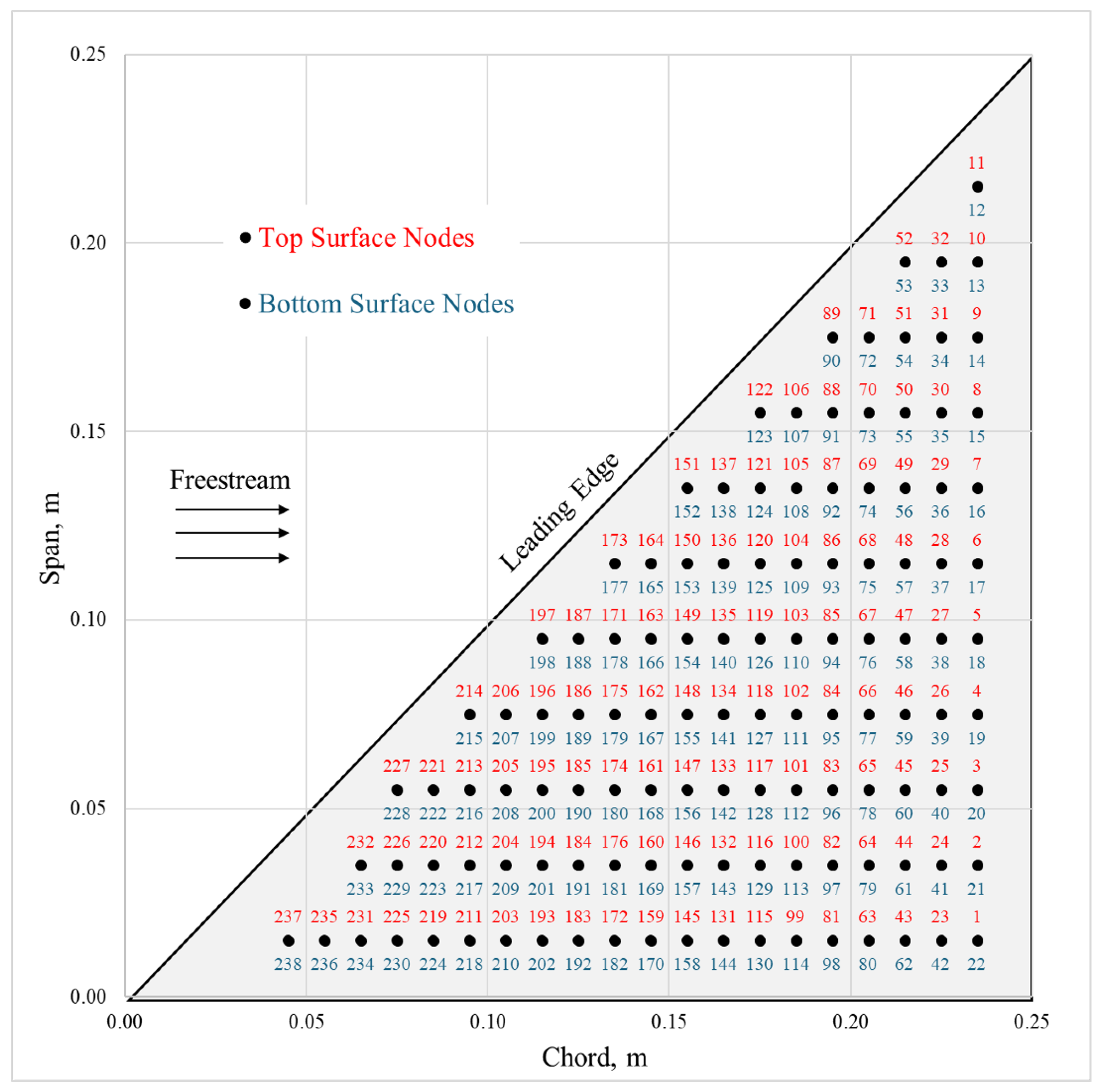
Velocity magnitude (not direction, since many AHS types are isotropic [22] and many natural flow-sensing systems measure only velocity [52]) was calculated at 0.5 cm, 1.0 cm, and 2.0 cm above the surface along eleven chordwise slices of the wing (Figure 2). This resulted in a three-layer shell of velocity data from which were extracted data sets with variable AHS height at 238 nodes (candidate sensor locations) over the top and bottom surfaces of the wing (Figure 3). This allowed SSPOP analysis for three fixed-height cases as well as a variable height case, which corresponds to real-world AHSs in which the length of the hair may be tuned during manufacturing or installation to account for different sensitivities [35,53]. Nodes were spaced at least 1 cm apart to account for mounting of neighboring sensors.
Nodes can be considered binary variables. For any given DP with Q sensors and N nodes, there will be Q local measurements and N Q nodes with null measurements; the DP surface velocity distribution is sparse while the full data set is semi-continuous. When a linear regression is performed on the variation of velocity at each DP node over a range of conditions, the prediction model will have Q nonzero coefficients and N Q coefficients of zero value. The solution space poses a combinatorial problem: for any given Q and N there are N ! Q ! ( N Q ) ! possible DPs. For small models with few sensors and relatively few nodes, a brute force search of the design space can be performed to find the optimal DP. However, realistic models may have many billions of DPs, so a data-driven approach to find a near-optimal DP is necessary.

2.2. Finding and Testing the Design Point

The SSPOP algorithm bypasses this combinatorial problem by greatly reducing its dimensionality. SSPOP (Figure 4) uses singular value decomposition (SVD) and linear discriminant analysis (LDA) to identify a sparse set of sensor locations (a Design Point, DP) at which most of the information from the flow may be obtained. It begins with SVD of the near-surface velocity magnitude data to identify prominent flow field features and create a low-rank approximation of the original data set. The data is then truncated using a weights matrix via LDA based on the variances of the original data. The highly truncated data sets contain well over 95 % of the information of the full dataset. A convex solver then creates the final sensor matrix and identifies the corresponding DP. Finally, linear regression of velocity data at the DP sensor locations is performed to obtain a root mean square error (RMSE) of prediction for any flight parameter (in this research, we predict α ). It should be emphasized that the SSPOP DP is application agnostic; the algorithm selects the most information-rich DP regardless of what that information will be used to predict. The RMSE between the original data (CFD simulation) and the sparsely calculated linear regression prediction is the performance metric of the DP. To determine its proximity to optimality, the performance of the SSPOP DP in terms of predictive accuracy was evaluated by comparison with the best possible DP found by a brute force search of all possible DPs for small Q values. For smaller models, the SSPOP DP can be ranked against every possible DP by performing a brute force combinatorial regression analysis. Analysis by this method is limited to low Q, especially when N is large. Once validated in general, the predictive performance of any SSPOP DP can be used to baseline a search of all possible DPs for a given model. See Section 5 for a link to supplementary information including the Matlab code and detailed flow chart for the SSPOP algorithm.

3. Results

The SSPOP algorithm found a DP for one through four sensors for each of the three single-length AHS models, and for one through three sensors for the variable-length model. A simple search was performed to improve the SSPOP performance, and all cases were compared against the best possible DP found by brute force search. The results are presented in Table 1 and described below, followed by a comparison of SSPOP against conventional optimization methods for one through ten sensors for each model.

3.1. Design Points and Predictive Performance

The predictive performance by RMSE of α and relative ranking of the SSPOP, SSPOP + Search, and Best Possible (BP) DPs are given in Figure 5. Among the single-length cases, the 1 cm AHS case performed best in all metrics for the 3- and 4-sensor DPs. This may have been anticipated as the airflow at this height may contain a wider range of information from both within and outside the boundary layer, compared with the shorter or longer hairs which may be too far under the viscous boundary or too far into the freestream, respectively. Also, as expected, the variable length model had the best brute-force optimum performance for all Q, due to having a design space three times as large. Unexpectedly, however, the 1 cm model outperformed the variable model in SSPOP and SSPOP + Search for the 3-sensor case, possibly due to the greater complexity of the variable dataset. In the brute force search three sensor case, the variable model retained one of the 1 cm hair nodes but replaced the other two with 2 cm hairs in nearly the same location but on the opposite surface. These changes in the variable model did not result in a significant improvement in performance (0.043 versus 0.039 RMSE α ) over the 1 cm model. This result indicates that the performance gains, if any, from variable length AHS models might not be worth the cost of manufacturing hairs of various lengths. Identifying a single ideal hair length for a given airfoil or wing may be advantageous. The SSPOP algorithm can assist in optimizing hair length through rapid iterations of different hair length models.
The SSPOP + Search results suggest diminishing returns with this method as Q increases. As the size of the design space increases, the rate of gain beyond the SSPOP performance by searching the design space slows considerably. This indicates that the SSPOP + Search method might not add value to SSPOP alone in very large models. For instance, the 3 sensor SSPOP + Search case did worse than the 2 sensor case. This is because the search was more difficult in higher dimensions, so even though the 3 sensor case started with a better SSPOP solution, the search did not improve the solution enough and it fell behind.
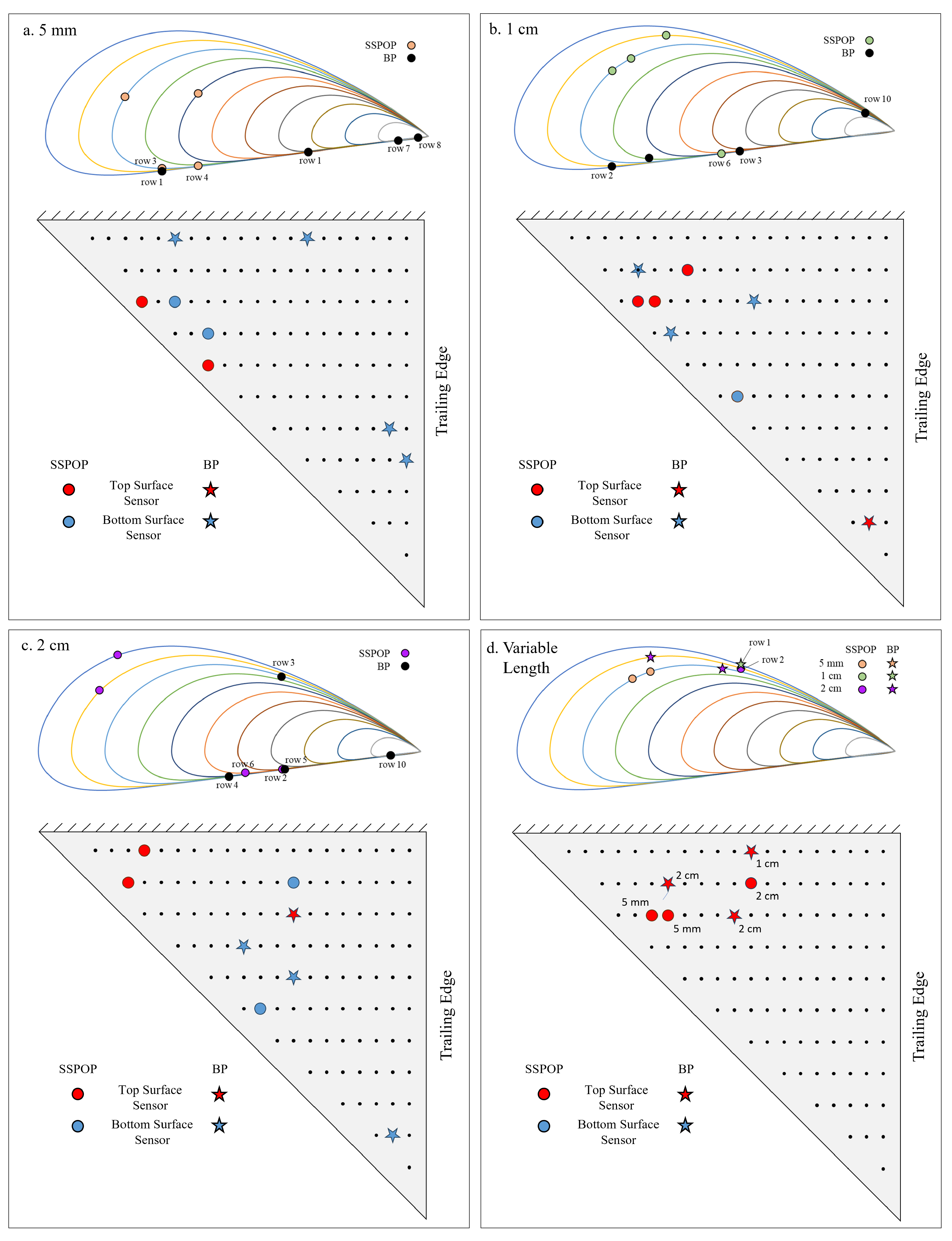
Figure 6 depicts the sensor locations for the SSPOP and BP DPs. Each row represents a chordwise slice, with Row 1 nearest the wing root and Row 11 nearest the wing tip. The thickness of the NACA 4415 airfoil is exaggerated by 300 % to facilitate visualization. The BP DP was found for up to four sensors for each fixed hair length case. The variable hair length case was only characterized for three sensors because the design space (238 nodes x 3 lengths = 714 variables and 10,738,066,626 DPs for a four-sensor solution) was too large for a brute force search. The SSPOP DPs for all single-length models (a-c) included multiple sensors near the leading edge, while the BP sensor locations were, on average, closer to the trailing edge. The single-length BP DPs tended to include sensors in more extreme locations, nearer the wingtip and trailing edge. However, the SSPOP DPs were more likely to include neighboring sensors. The variable length model (d) featured the closest agreement between the SSPOP DP and the BP DP. Two-thirds of the SSPOP sensors were located on the top surface, compared to only one-third of the BP sensors.

3.2. SSPOP versus Conventional Optimization

The simplicity and efficiency of the SSPOP algorithm is a major driver in its use for sensor placement optimization over conventional approaches. Below we first compare SSPOP DP performance against greedy search (GS) and then against gradient-based optimization using auto-differentiation, evaluating the costs and benefits of each method.

3.2.1. Greedy Search

A GS optimization algorithm first finds the best single-sensor solution, then finds the best two-sensor solution in which the location of the first sensor is retained, and so on. The benefits of a GS is its simplicity and speed, and there is no upper limit for any realistic model in terms of node and sensor quantity. For a model with linear regression such as used here, each iteration of the search has negligible cost, and the total cost of the GS is also negligible. The question is whether GS reliably arrives at a near-optimal solution for any Q. We cannot know with certainty whether a GS solution approaches the optimum unless we compare it to a brute force search, but this is infeasible for models with high Q and high N. However, having shown that the SSPOP solutions are within the top 1 % of all possible solutions where the design space can be characterized, we can confidently compare the relative performance of SSPOP and GS solutions for any number of sensors.
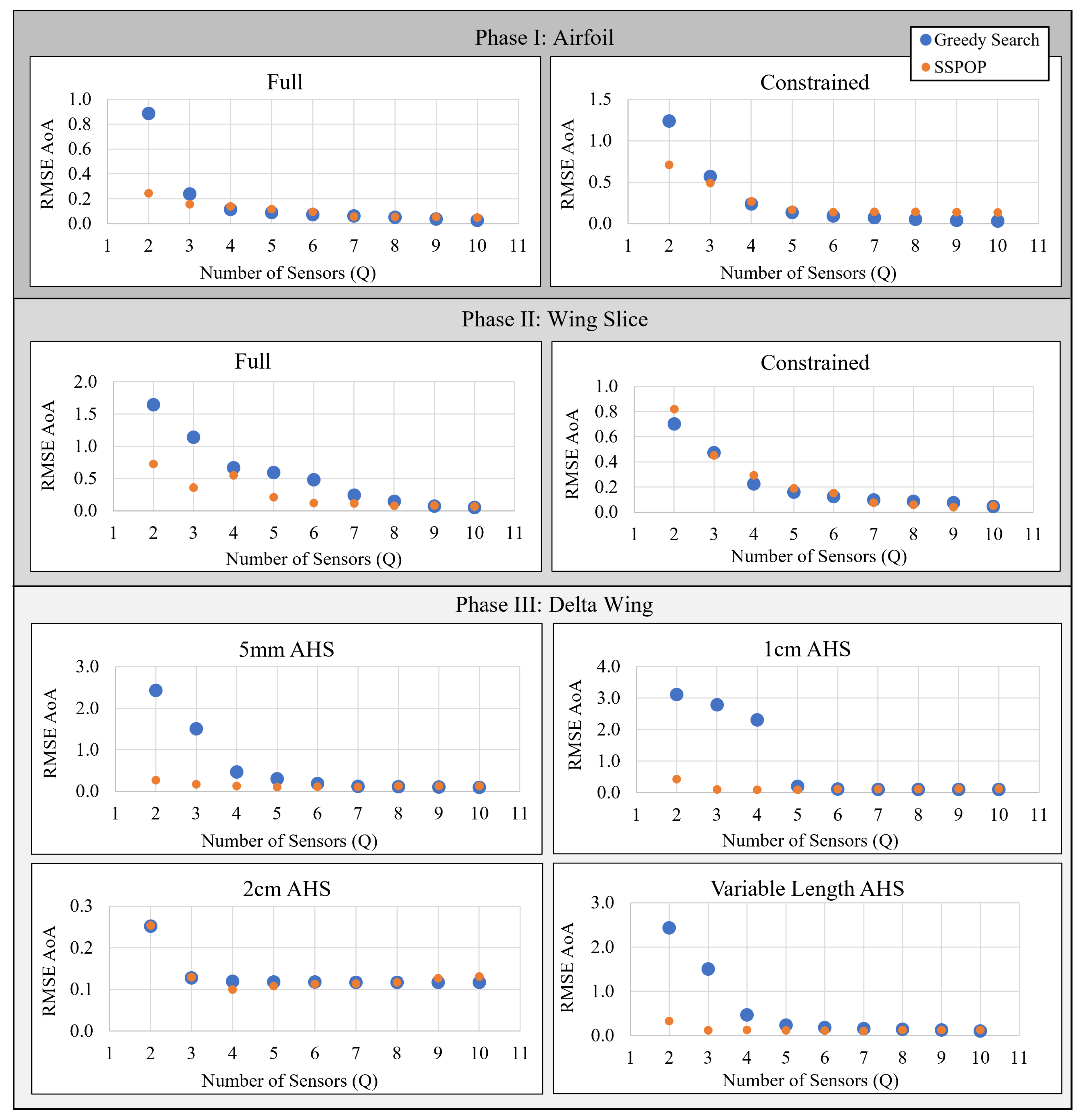
Figure 7 plots the predictive performances of the SSPOP and GS DPs for one through ten sensors for an airfoil model and 2D slice of a wing (model from [23]), and the 3D wing of the present study. In most cases, the SSPOP solution outperforms the GS solution, especially at lower Q. In other instances at low Q, and in all cases for high Q, the GS solution approximately matches the SSPOP solution. In no case does the GS solution significantly outperform the SSPOP solution.
Based on these results, it is evident that a GS can yield a top-one-percent result, especially at higher Q values, but some form of validation would be required to confirm this for each model. We have shown in [23] and above that SSPOP reliably finds a top-one-percent solution regardless of model in both 2D and 3D for two or more sensors. The two approaches may be used together, just as we have done earlier with SSPOP + Search. The SSPOP + GS would first run SSPOP to establish a goal, and either a GS or simple search, or both, could be run to seek improvement. From Figure 8, it is evident that the SSPOP + Search approach delivers diminished returns as Q increases, due to the exponentially increased design space at larger Q. Therefore, for very large models, it may be sufficient to simply keep the SSPOP DP without additional searches.
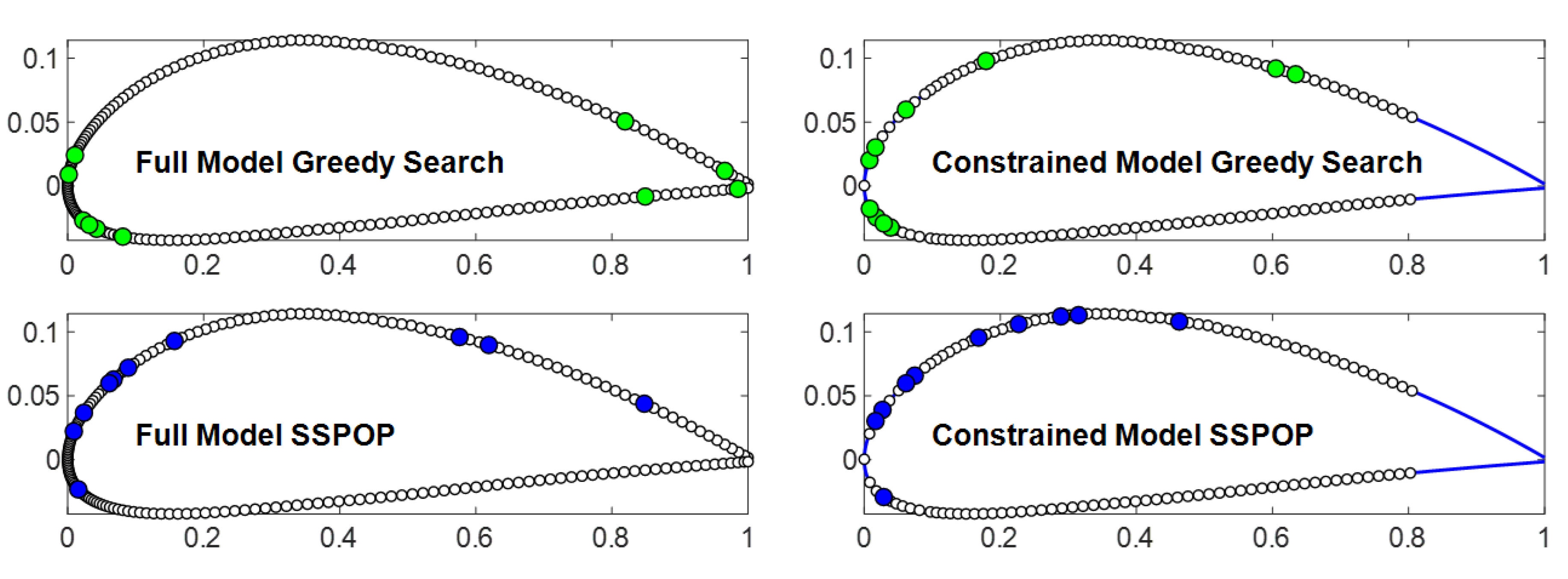
It may also be the case that the data-driven SSPOP algorithm is less sensitive to model configuration than the GS. Figure 8 shows the ten-sensor GS and SSPOP DPs for two variations of an airfoil model. Compared with SSPOP, the GS more significantly exploits the extreme conditions at the leading and trailing edges, especially for the full model. Tight groupings which may be impractical for real-world sensor installation are more prevalent in the GS DPs. In addition, GS is sensitive to local minima in the objective function, which may lead to early ’mistakes’ in node selection which impact the higher-Q models. For example, the best single-sensor solution is highly variable in performance and tends to be located at extreme points. In a GS, this sensor must be retained whether it is helpful in combination with the others or not.

3.2.2. Other Conventional Optimization Approaches

The SSPOP and brute force methods formulate the sensor placements as a discrete problem, where the sensors must be placed at specific node locations. However, it can also be formulated as a continuous problem by interpolating the velocities between the grid points. Given specific sensor locations, one can perform linear regression on the training cases and evaluate accuracy on the test cases. This entire pipeline of sensor locations → sensor velocities → linear regression to predict α from sensor velocities → predicting α in the test cases and finding the MSE was implemented in TensorFlow (Figure 9). This allows the gradients of α -prediction-error with respect to sensor locations to be found using auto-differentiation, enabling the application of gradient-based optimization algorithms.
Linear regression is performed using TensorFlow’s tf.linalg.lstsq function, which requires fast=True in order to be differentiable. However, this setting causes the linear regression to use Cholesky decomposition. While this method is less robust and stable than the complete orthogonal decomposition used when fast=False, an L2 regularization of 10 7 aided numerical stability.
Sensor locations were constrained to always remain within the appropriate region of the airfoil surface. Whenever a sensor moved outside of the feasible region, it was both penalized and moved to within the sensor region before linear regression was performed, ensuring the optimizer settled on a feasible solution.
The continuous optimization formulation introduces a limitation not found in the discrete optimization or SSPOP. Because sensors cannot be added too close to the leading or trailing wing edges, the feasible regions on the top and bottom of the wing are separated. This means sensors will remain confined within their initial regions. To handle this, we run two different optimizations for each hair length case, one with all three discrete variable length sensors on the top of the wing and one with all three discrete variable length sensors on the bottom.
Two optimization algorithms for sensor placement were initially considered: Adam (Adaptive moment estimation) and BFGS (Broyden–Fletcher–Goldfarb–Shanno). It was found that Adam is less reliable than BFGS for this use case. The Adam solution tends to fluctuate unpredictably, and can move away from a good solution without returning. This behavior is useful when training a neural network with thousands-to-billions of parameters, where the parameter space is full of nearly-equally-good local optima and the most important thing is to avoid getting stuck at one of the many saddle points. However, in engineering applications BFGS performs better. Therefore, only BFGS results are compared to SSPOP. For implementation, we used SciPy’s L-BFGS-B function, where the L stands for limited memory and the B stands for box constraints (where each variable is constrained by a minimum and maximum value). BFGS approximates the Hessian of the loss function using gradients calculated with auto-differentiation.
In total, we ran four cases, with 5 mm, 1 cm, 2 cm, and variable length hairs. For this last case, the hair lengths were optimized as continuous variables. Because BFGS is not a global optimization method, it was run multiple times. For each optimization case, 10 different initial sensor placements were selected using Latin Hypercube Sampling, a BFGS optimization run was conducted for each initial sensor placement, and the best optimum from the 10 results was selected as the final optimum. Finally, the sensors at this final continuous optimization are snapped to the nearest grid points. In cases where one or more sensors are nearly equidistant from multiple grid points, all combinations of nearby grid points are tested and the best configuration selected. All results are shown in Table 2. BFGS outperforms SSPOP in the 5 mm case, but performs worse in the other three cases.
Snapping the sensors to the grid resulted in varying levels of degradation for the α prediction accuracy. For instance, in the case with 5 mm hairs on top of the wing, test error increased negligibly from 0 . 143 to 0 . 145 . At the other extreme, adjusting the 1 cm sensors on the top of the wing increased error from 0 . 137 to 0 . 514 , or a factor of around four.
On average, each of the 10 optimization runs for each case takes 15-20 seconds to complete, making the method fast to execute. This makes BFGS comparable in speed to SSPOP, even if the optimization is repeated 10 times to increase the chance of finding the global optimum.
On the other hand, BFGS with auto-differentiation also comes with drawbacks in this application. First, it is more difficult and time-consuming to implement than SSPOP, requiring interpolation of air velocity values, geometric constraints on sensor locations, a differentiable implementation of linear regression, and the testing of multiple combinations of nearby grid points once optimization converges. While none of these individually are too difficult to implement, they do take time which is not required when implementing SSPOP. Second, each sensor is constrained to its initial region. While this can be handled by running optimization cases for every possible combination of sensors in every region, this scales poorly as the number of sensors and number of regions increases. Finally, as previously mentioned, the accuracy of the final BFGS solution is often highly sensitive to small perturbations in the sensor location and may be sensitive to initial sensor location choice, unlike SSPOP. Despite these drawbacks, BFGS with auto-differentiation performed only slightly worse than SSPOP in this example, and either method is powerful enough to handle sensor placement optimization.

4. Discussion

The SSPOP algorithm is capable of quickly finding a DP of AHS placements which predicts α by linear regression to well within 0.10 accuracy over a wide range of α for 3D wings. The performance of these SSPOP DPs generally ranks within the top 1 % of all possible DPs for those cases where a brute force analysis was performed, granting confidence that similar performance can be expected for any arbitrary number of sensors and nodes on a wing of any shape and size. Therefore, in large models for which a brute force search is infeasible and the true optimum DP cannot be found, we can use the SSPOP DP as a top-one-percent solution starting point. If needed, a search can then be performed to find a DP which performs up to an order of magnitude better. These results have significant implications for bioinspired aircraft design, sensor design and placement, and FBF control system design.

4.1. SSPOP and Flight-by-Feel

In general, the achievable predictive accuracy improves with increasing number of sensors Q. However, the predictive performance varies significantly across the possible DPs for a given Q and N. In order to find a DP suitable for FBF, an objective maximum RMSE (for AoA or any flight parameter) may be set based on the requirements of the FBF controller and desired performance. In the present work, no RMSE performance objective was given other than to find the best possible performance subject to the constraints of the solution method. We have shown that the SSPOP algorithm can quickly predict the near-optimal performance of any number of sensors on a wing, so a flight control designer could incorporate these metrics into a tradeoff analysis for the number of sensors. After performing SSPOP for a range of Q (as in Figure 7), the DP with the lowest Q meeting a control-system-driven predictive accuracy requirement would be considered the optimum for the given criteria. Comprehensive FBF systems for future autonomous aircraft might benefit from a combination of sensor placement optimization approaches for different sensor types and modalities. For example, a flapping-wing MAV might use strain sensors placed by an observability analysis optimization approach on the wings for wing state estimation [54], SSPOP could optimally place hair sensors on the body for flight state estimation, bioinspired isolators could protect sensitive navigation equipment [55], and nano-scale hair sensors could be used for inertial and directional control [56].

4.2. SSPOP and Aircraft Design

SSPOP only requires a discrete dataset of flow, pressure, or other metrics, which can be found by computer modeling (such as CFD) or wind tunnel testing (such as particle image velocimetry). Therefore, SSPOP can be used early and often in the design process, helping to determine the required number and placement of sensors even as early as the conceptual design stage. The flexibility and robustness of the SSPOP algorithm is potentially a major advantage over a conventional sensor placement optimization approach, especially early in the design process when configurations are subject to significant change. Unlike a conventional approach in which sensors are placed only after the aircraft design is fixed, a bioinspired FBF design approach can use SSPOP to ensure the appropriate sensors are seamlessly integrated into the skin of the aircraft in a near-optimal location. Likewise, the form and structure of an AHS itself may be varied early in the design process, as we have done with our variable hair length model. Just as we observe in the hair sensors of natural fliers, an AHS should be fine-tuned to suit the perception needs for flight control based on its location and envelope of flight conditions [53,57].

5. Conclusions

This research covered the application of a data-driven approach for identifying a near-optimal location of a sparse set of velocity magnitude sensors for predicting the angle of attack of a wing. The primary model was a canonical NACA 4415 45-swept blunt-edged delta wing. The performance of the DP selected by the SSPOP algorithm was compared, where possible, to the true optimum DP found by brute force search. For two or more sensors, the SSPOP DP ranked within or near the top 1 % of all possible DPs by RMSE. Adding a search procedure after SSPOP yielded a DP well within the top 0.01 % in a few minutes versus the several hours required for a brute force search for these relatively small models. The SSPOP algorithm is highly adaptable, having been previously demonstrated on 2D models and here on three fixed-length AHS models and one variable-length AHS model, and performing well in all cases. Therefore, SSPOP can be applied in two or three dimensions for any shape and node configuration and for pressure, strain, or any other FBF-relevant sensors. Unlike some conventional optimization techniques, SSPOP does not depend on node/region continuity, allows discrete flow data, and is not sensitive to initial conditions. Additionally, in our analysis, SSPOP proved to be slightly more accurate than BFGS with auto-differentiation. By quickly and easily guiding the placement of sensors for near-optimum predictive accuracy, the SSPOP algorithm can support the implementation of FBF control in the design and operation of next-generation aircraft. The success of SSPOP for bioinspired FBF control suggests the applicability of bioinspiration in aircraft design extends far beyond its current horizons.

Author Contributions

Conceptualization, A.H.; methodology, A.H. and A.B.; validation, A.H.; resources, all; writing—original draft preparation, A.H. and A.B.; writing—review and editing, all. All authors have read and agreed to the published version of the manuscript.

Funding

This research was supported in part by an appointment to the NRC Research Associateship Program at the Air Force Institute of Technology, administered by the Fellowships Office of the National Academies of Sciences, Engineering, and Medicine. The contract number for the program is FA955024CB001. The APC was funded by the Air Force Institute of Technology.

Institutional Review Board Statement

Not applicable.

Data Availability Statement

A Matlab code supplement is available [58] for reproducing some of the results in this manuscript, including the SSPOP algorithm code, example flow datasets, and detailed flow charts of the SSPOP algorithm.

Acknowledgments

The views and conclusions contained herein are those of the authors and do not necessarily represent official policies or endorsements, either expressed or implied, of the U.S. Air Force, the U.S. Department of Defense, or the U.S. Government. This paper is cleared for public release, case number 88ABW-2024-0680. This material is declared a work of the U.S. Government and is not subject to copyright protection in the United States.

Conflicts of Interest

The authors declare no conflicts of interest. The funders had no role in the design of the study; in the collection, analyses, or interpretation of data; in the writing of the manuscript; or in the decision to publish the results.

References

  1. Usherwood, J.R.; Cheney, J.A.; Song, J.; Windsor, S.P.; Stevenson, J.P.; Dierksheide, U.; Nila, A.; Bomphrey, R.J. High aerodynamic lift from the tail reduces drag in gliding raptors. Journal of Experimental Biology 2020, 223. [Google Scholar] [CrossRef]
  2. Harvey, C.; Baliga, V.B.; Wong, J.C.; Altshuler, D.L.; Inman, D.J. Birds can transition between stable and unstable states via wing morphing. Nature 2022, 603, 648–653. [Google Scholar] [CrossRef]
  3. Taylor, G.K.; Thomas, A.L.R. Evolutionary Biomechanics: Selection, Phylogeny, and Constraint; Oxford series in ecology and evolution; Oxford University Press: Oxford, UK, 2014. [Google Scholar]
  4. Taylor, G.K.; Carruthers, A.C.; Hubel, T.Y.; Walker, S.M. Wing Morphing in Insects, Birds and Bats: Mechanism and Function. In Morphing Aerospace Vehicles and Structures, 1st ed.; John Valasek., Ed.; John Wiley & Sons, Ltd., 2012; pp. 13–40.
  5. Gillies, J.A.; Thomas, A.L.; Taylor, G.K. Soaring and manoeuvring flight of a steppe eagle Aquila nipalensis. Journal of Avian Biology 2011, 42, 377–386. [Google Scholar] [CrossRef]
  6. Tuthill, J. Begrudging the bat. Journal of Experimental Biology 2015, 218, 2318–2319. [Google Scholar] [CrossRef]
  7. Wang, S.; Zhang, X.; He, G.; Liu, T. Lift enhancement by bats’ dynamically changing wingspan. Journal of the Royal Society Interface 2015, 12. [Google Scholar] [CrossRef]
  8. Ruland, O.; Mkhoyan, T.; De Breuker, R.; Wang, X. Black-box Online Aerodynamic Performance Optimization for a Seamless Wing with Distributed Morphing. AIAA SciTech Forum; , 2022. doi:10.2514/6.2022-1840.
  9. Burgess, S. Universal optimal design in the vertebrate limb pattern and lessons for bioinspired design. Bioinspiration & Biomimetics 2024, 19, 051004. [Google Scholar] [CrossRef]
  10. Bardera, R.; Rodriguez-Sevillano, A.A.; Barroso Barderas, E.; Matias Garcia, J.C. Computational Study of Aerodynamic Effects of the Dihedral and Angle of Attack of Biomimetic Grids Installed on a Mini UAV. Biomimetics 2024, 9, 12. [Google Scholar] [CrossRef]
  11. Lentink, D. Coevolving advances in animal flight and aerial robotics. Interface Focus 2017, 7. [Google Scholar] [CrossRef]
  12. Martin-Silverstone, E.; Habib, M.B.; Hone, D.W. Volant Fossil Vertebrates: Potential for Bioinspired Flight Technology. Trends in Ecology and Evolution 2020, 35, 618–629. [Google Scholar] [CrossRef]
  13. Salowitz, N.; Guo, Z.; Li, Y.H.; Kim, K.; Lanzara, G.; Chang, F.K. Bio-inspired stretchable network-based intelligent composites. Journal of Composite Materials 2013, 47, 97–105. [Google Scholar] [CrossRef]
  14. Chahl, J.; Chitsaz, N.; McIvor, B.; Ogunwa, T.; Kok, J.M.; McIntyre, T.; Abdullah, E. Biomimetic drones inspired by dragonflies will require a systems based approach and insights from biology. Drones 2021, 5. [Google Scholar] [CrossRef]
  15. Naigle, S.C.; Hiltner, S.D.; Walker, M.M. Numerical Optimization of a Vortex Generating Jet on a Non-Slender Delta Wing. AIAA SciTech Forum;, 2022. [CrossRef]
  16. Chen, L.; Zhang, Y.; Zhou, C.; Wu, J. Aerodynamic mechanisms in bio-inspired micro air vehicles: A review in the light of novel compound layouts. IET Cyber-systems and Robotics 2019, 1, 2–12. [Google Scholar] [CrossRef]
  17. Sihite, E.N.; Lessieur, A.; Dangol, P.; Singhal, A.; Ramezani, A. Orientation stabilization in a bioinspired bat-robot using integrated mechanical intelligence and control. Proceedings SPIE Defense & Commercial Sensing; , 2021; Vol. 11758, pp. 12–20. doi:10.1117/12.2587894.
  18. Iida, F.; Nurzaman, S.G. Adaptation of sensor morphology: An integrative view of perception from biologically inspired robotics perspective. Interface Focus 2016, 6. [Google Scholar] [CrossRef]
  19. Chittka, L.; Brockmann, A. Perception space - The final frontier. PLoS Biology 2005, 3, 0564–0568. [Google Scholar] [CrossRef]
  20. Zikmund, P.; Macík, M.; Dvořák, P.; Míkovec, Z. Bio-inspired aircraft control. Aircraft Engineering and Aerospace Technology 2018, 90, 983–991. [Google Scholar] [CrossRef]
  21. Khot, N.S.; Veley, D.E.; Grandhi, R.V. Effect of number of actuators on optimum actively controlled structures. Engineering Optimization 1992, 19, 51–63. [Google Scholar] [CrossRef]
  22. Hollenbeck, A.C.; Grandhi, R.; Hansen, J.H.; Pankonien, A.M. Bioinspired Artificial Hair Sensors for Flight-by-Feel of Unmanned Aerial Vehicles: A Review. AIAA Journal 2023, 61, 5206–5231. [Google Scholar] [CrossRef]
  23. Hollenbeck, A.; Grandhi, R.V.; Hansen, J.; Pankonien, A.M. Sparse Sensor Placement Optimization for Prediction of Angle of Attack with Artificial Hair-Cell Airflow Microsensors. AIAA SciTech Forum; , 2024. doi:10.2514/6.2024-1798.
  24. Hollenbeck, A.C.; Grandhi, R.; Hansen, J.H.; Pankonien, A.M. Sparse Flow Sensor Placement Optimization for Flight-by-Feel Control of 2D Airfoils. AIAA Journal 2024, pp. 1–10. doi:10.2514/1.J064040.
  25. Yang, X.S. Nature-inspired optimization algorithms: Challenges and open problems. Journal of Computational Science 2020, 46, 101104. [Google Scholar] [CrossRef]
  26. Brunton, B.W.; Brunton, S.L.; Proctor, J.L.; Kutz, J.N. Sparse Sensor Placement Optimization for Classification. SIAM Journal on Applied Mathematics 2016, 76, 2099–2122. [Google Scholar] [CrossRef]
  27. Mohren, T.L.; Daniel, T.L.; Brunton, S.L.; Brunton, B.W. Neural-inspired sensors enable sparse, efficient classification of spatiotemporal data. Proceedings of the National Academy of Sciences of the United States of America 2018, 115, 10564–10569. [Google Scholar] [CrossRef]
  28. Manohar, K.; Brunton, B.W.; Kutz, J.N.; Brunton, S.L. Data-Driven Sparse Sensor Placement for Reconstruction: Demonstrating the Benefits of Exploiting Known Patterns. IEEE Control Systems 2018, 38, 63–86. [Google Scholar] [CrossRef]
  29. Callaham, J.; Maeda, K.; Brunton, S.L. Robust flow field reconstruction from limited measurements via sparse representation. Physical Review Fluids 2019, 4, 103907. [Google Scholar] [CrossRef]
  30. Brunton, B.W.; Botvinick, M.M.; Brody, C.D. Rats and Humans Can Optimally Accumulate Evidence for Decision-Making. Science 2013, 340, 95–98. [Google Scholar] [CrossRef]
  31. Bright, I.; Lin, G.; Kutz, J.N. Compressive sensing based machine learning strategy for characterizing the flow around a cylinder with limited pressure measurements. Physics of Fluids 2013, 25, 127102. [Google Scholar] [CrossRef]
  32. Aiello, B.R.; Stanchak, K.E.; Weber, A.I.; Deora, T.; Sponberg, S.; Brunton, B.W. Spatial distribution of campaniform sensilla mechanosensors on wings: Form, function, and phylogeny. Current Opinion in Insect Science 2021, 48, 8–17. [Google Scholar] [CrossRef]
  33. Hinson, B.T.; Morgansen, K.A. Gyroscopic sensing in the wings of the hawkmoth Manduca sexta: The role of sensor location and directional sensitivity. Bioinspiration and Biomimetics 2015, 10. [Google Scholar] [CrossRef]
  34. Sterbing-D’Angelo, S.J.; Liu, H.; Yu, M.; Moss, C.F. Morphology and deflection properties of bat wing sensory hairs: Scanning electron microscopy, laser scanning vibrometry, and mechanics model. Bioinspiration and Biomimetics 2016, 11. [Google Scholar] [CrossRef]
  35. Slinker, K.A.; Kondash, C.; Dickinson, B.T.; Baur, J.W. CNT-Based Artificial Hair Sensors for Predictable Boundary Layer Air Flow Sensing. Advanced Materials Technologies 2016, 1. [Google Scholar] [CrossRef]
  36. Izquierdo, J.J.; Hollenbeck, A.; Demott, R.; Bramlette, R.; Cervantes, G.; Vallejo, C.; Kudva, J. Improving synthesis and testing conditions for bio-inspired carbon nanotube artificial hair sensors: Design, construction, reproduction, and calibration. AIAA Scitech 2024 Forum; , 2024. doi:10.2514/6.2024-0259.
  37. Dickinson, B.T.; Singler, J.R.; Batten, B.A. The Detection of Unsteady Flow Separation with Bioinspired Hair-Cell Sensors. 26th AIAA Aerodynamic Measurement Technology and Ground Testing Conference; , 2008. doi:10.2514/6.2008-3937.
  38. Dickinson, B.T. Hair receptor sensitivity to changes in laminar boundary layer shape. Bioinspiration and Biomimetics 2010, 5. [Google Scholar] [CrossRef]
  39. Court, A.; Bruecker, C. Fly by Feel: Flow Event Detection via Bioinspired Wind-Hairs. Fluids 2024, Vol. 9, Page 74 2024, 9, 74. [Google Scholar] [CrossRef]
  40. Ellington, C.P.; van den Berg, C.; Willmott, A.P.; Thomas, A.L.R. Leading-edge vortices in insect flight. Nature 1996, 384, 626–630. [Google Scholar] [CrossRef]
  41. Warrick, D.R.; Tobalske, B.W.; Powers, D.R. Lift production in the hovering hummingbird. Proceedings of the Royal Society B: Biological Sciences 2009, 276, 3747–3752. [Google Scholar] [CrossRef]
  42. Linehan, T.; Mohseni, K. Scaling trends of bird’s alular feathers in connection to leading-edge vortex flow over hand-wing. Scientific Reports 2020, 10. [Google Scholar] [CrossRef]
  43. Muijres, F.T.; Johansson, L.C.; Barfield, R.; Wolf, M.; Spedding, G.R.; Hedenström, A. Leading-Edge Vortex Improves Lift in Slow-Flying Bats. Science 2008, 319, 1250–1253. [Google Scholar] [CrossRef]
  44. Lentink, D.; Dickson, W.B.; Van Leeuwen, J.L.; Dickinson, M.H. Leading-Edge Vortices Elevate Lift of Autorotating Plant Seeds. Science 2009, 324, 1438–1440. [Google Scholar] [CrossRef]
  45. Bomphrey, R.J. Insects in flight: Direct visualization and flow measurements. Bioinspiration & Biomimetics 2006, 1, S1. [Google Scholar] [CrossRef]
  46. KleinHeerenbrink, M.; Christoffer Johansson, L.; Hedenström, A. Multi-cored vortices support function of slotted wing tips of birds in gliding and flapping flight. Journal of the Royal Society Interface 2017, 14. [Google Scholar] [CrossRef]
  47. Malicki, L.; Malecha, Z.; Tomczuk, K. Leading-Edge Vortex Controller (LEVCON) Influence on the Aerodynamic Characteristics of a Modern Fighter Jet. Energies 2023, 16, 7590. [Google Scholar] [CrossRef]
  48. Zhang, S.; Jaworski, A.J.; McParlin, S.C.; Turner, J.T. Experimental investigation of the flow structures over a 40 swept wing. Aeronautical Journal 2019, 123, 39–55. [Google Scholar] [CrossRef]
  49. Thomas, A.L.; Taylor, G.K.; Srygley, R.B.; Nudds, R.L.; Bomphrey, R.J. Dragonfly flight: Free-flight and tethered flow visualizations reveal a diverse array of unsteady lift generating mechanisms, controlled primarily via angle of attack. J. Exp. Biol. 2004, 207, 4299–4323. [Google Scholar] [CrossRef]
  50. Sutrisno, S.; Deendarlianto, D.; Rohmat, T.A.; Wibowo, S.B.; Iswahyudi, S. Vortex Dynamics Analysis of Straight-Body-Type-Fuselage Fighter Using CFD Simulation. Journal of Aerospace Technology and Management 2020, 12. [Google Scholar] [CrossRef]
  51. Demoret, A.C. The Effect of Passive and Active Boundary-layer Fences on Delta Wing Performance at Low Reynolds Number. Theses and Dissertations; Air Force Institute of Technology, Air Force Institute of Technology: Wright Patterson Air Force Base, Ohio, 2020; Volume 3213. [Google Scholar]
  52. Colvert, B.; Chen, K.K.; Kanso, E. Bioinspired Sensory Systems for Shear Flow Detection. Journal of Nonlinear Science 2017, 27, 1183–1192. [Google Scholar] [CrossRef]
  53. Slinker, K.; Kondash, C.; Dickinson, B.; Baur, J. High-Bandwidth and Sensitive Air Flow Sensing Based on Resonance Properties of CNT-on-Fiber Hairs. Journal of Carbon Research 2017, 3. [Google Scholar] [CrossRef]
  54. Jin, B.; Xu, H.; Peng, J.; Lu, K.; Lu, Y. Derivative-Free Observability Analysis for Sensor Placement Optimization of Bioinspired Flexible Flapping Wing System. Biomimetics 2022, 7, 178. [Google Scholar] [CrossRef]
  55. Zhang, Y.; Wang, L.; Li, L.; Wang, X.; He, S. Modeling and Analysis of Bio-Inspired, Reconfigurable, Piezo-Driven Vibration Isolator for Spacecraft. Biomimetics 2024, 9, 29. [Google Scholar] [CrossRef]
  56. Moshizi, S.A.; Pastras, C.J.; Peng, S.; Wu, S.; Asadnia, M. Artificial Hair Cell Sensor Based on Nanofiber-Reinforced Thin Metal Films. Biomimetics 2024, 9, 18. [Google Scholar] [CrossRef]
  57. Su, W.; Reich, G.W. Geometric scaling of artificial hair sensors for flow measurement under different conditions. Smart Materials and Structures 2017, 26, 037002. [Google Scholar] [CrossRef]
  58. Hollenbeck, A.C. SSPOP (Sparse Sensor Placement Optimization for Prediction) Code and Figure Supplement, 2024.
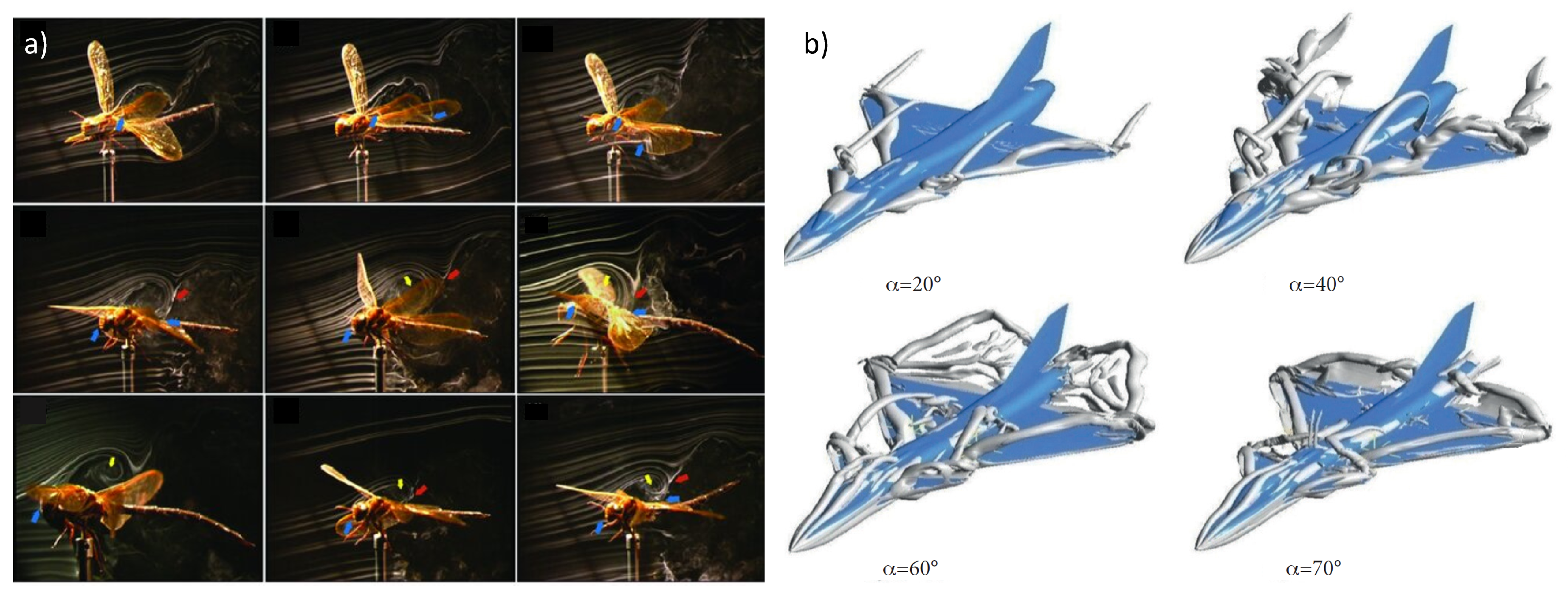
Figure 1. Lift-inducing LEV formation and evolution in (a) flapping dragonfly wings (from [49]) and (b) a delta-canard fighter at high AoA (from [50]).
Preprints 117084 g001
Figure 2. 45 deg sweep, NACA 4415 delta wing model. (a) Full data matrix of airflow velocity magnitude for the 1cm hair length model at each of 238 nodes over 40 angles of attack from -10 to 20. (b) CFD: Velocity magnitude at three heights above wing for eleven slices at α = 20 .
Preprints 117084 g002
Figure 3. Node locations and numbers. There are 238 nodes spaced evenly over the top and bottom surfaces.
Preprints 117084 g003
Figure 4. The Sparse Sensor Placement Optimization for Prediction (SSPOP) algorithm. From [23].
Preprints 117084 g004
Figure 5. Performance and ranking for the three individual hair length models and the variable hair length model.
Preprints 117084 g005
Figure 6. Design Points for SSPOP and best possible with four sensors for (a) 5 mm, (b) 1 cm, (c) 2 cm, and (d) three sensors for variable AHS hair lengths.
Preprints 117084 g006
Figure 7. DP performance (degrees AoA prediction) of a Greedy Search and SSPOP for two through ten sensors.
Preprints 117084 g007
Figure 8. Ten-sensor design points for SSPOP and Greedy Search solutions for a 2D airfoil (model from [23].)
Preprints 117084 g008
Figure 9. Flowchart of auto-differentiated sequential data processing.
Preprints 117084 g009
Table 1. Design Points, Performance, and Ranking for three single-hair-length models and one model with variable hair length. Nodes for the variable model are colored according to their length.
SSPOP SSPOP + Search Best Possible
Q DP RMSE
(deg)
Rank
(%)
DP RMSE
(deg)
Rank
(%)
DP RMSE
(deg)
5 cm 1 227 7.517 2.521 13 7.105
2 216 227 0.271 0.177 183 211 0.142 0.004 183 211 0.142
3 43 227 228 0.170 0.231 188 193 225 0.137 0.008 130 198 207 0.095
4 197 199 216 227 0.131 0.105 130 142 158 232 0.125 0.055 15 36 130 218 0.045
1 cm 1 227 7.756 1.261 227 7.493
2 215 227 0.426 3.865 21 224 0.125 0.004 210 224 0.125
3 153 213 232 0.106 0.048 156 161 223 0.060 0.000 145 167 208 0.043
4 165 194 213 221 0.092 0.057 86 93 210 223 0.075 0.012 32 156 207 223 0.036
2 cm 1 227 8.009 0.420 227 8.009
2 133 199 0.254 0.450 145 230 0.161 0.004 145 230 0.161
3 141 180 214 0.129 0.091 155 200 220 0.064 0.000 33 96 188 0.056
4 143 165 225 232 0.100 0.111 112 157 189 218 0.088 0.042 33 133 140 178 0.038
Var. 1 227 7.517 0.980 13 7.105
2 64 215 0.331 1.288 156 223 0.080 0.000 156 223 0.080
3 146 205 213 0.121 0.061 206 210 234 0.097 0.012 145 161 204 0.039
Table 2. Comparison of sensor locations and performance for optimum (brute-force search), full-surface SSPOP, and top- or bottom-only BFGS DPs. Rows are ordered from best-to-worst RMSE.
Method RMSE
deg α
DP nodes Method RMSE
deg α
DP nodes
5 mm BF Search 0.045 15 36 130 218 2 cm BF Search 0.038 33 133 140 178
BFGS (bot) 0.099 22 109 168 210 SSPOP 0.100 143 165 225 232
SSPOP 0.131 197 199 216 227 BFGS (top) 0.143 1 7 23 226
BFGS (top) 0.145 1 9 137 235 BFGS (bot) 0.150 57 93 125 217
1 cm BF Search 0.036 32 156 207 223 Var. BF Search 0.039 145 161 204
SSPOP 0.092 165 194 213 221 SSPOP 0.121 146 205 213
BFGS (bot) 0.141 40 41 140 190 BFGS (bot) 0.123 19 98 207
BFGS (top) 0.514 1 23 115 175 BFGS (top) 0.966 1 23 131
Disclaimer/Publisher’s Note: The statements, opinions and data contained in all publications are solely those of the individual author(s) and contributor(s) and not of MDPI and/or the editor(s). MDPI and/or the editor(s) disclaim responsibility for any injury to people or property resulting from any ideas, methods, instructions or products referred to in the content.
Copyright: This open access article is published under a Creative Commons CC BY 4.0 license, which permit the free download, distribution, and reuse, provided that the author and preprint are cited in any reuse.
Prerpints.org logo

Preprints.org is a free preprint server supported by MDPI in Basel, Switzerland.

Subscribe

© 2024 MDPI (Basel, Switzerland) unless otherwise stated