Finding a Published Research Paper Which Meaningfully Averages the Most Pathalogical Functions (v3)

1. Intro

Let $n\in \mathbb{N}$ and suppose function $f:A\subseteq {\mathbb{R}}^n\to \mathbb{R}$, where A and f are Borel. Let ${\dim }_{\mathrm{H}}(·)$ be the Hausdorff dimension, where ${\mathcal{H}}^{{\dim }_{\mathrm{H}}(·)}(·)$ is the Hausdorff measure in its dimension on the Borel $\sigma$-algebra.

1.1. First Special Case of f

If the graph of f is G, is there an explicit f where:

(1)

The function f is everywhere surjective [2] (i.e., function defined on a topological space where its’ restriction to any non-empty open subset is surjective).

(2)

${\mathcal{H}}^{{\dim }_{\mathrm{H}}\left(G\right)}\left(G\right)=0$

1.1.1. Potential Answer

If $A=\mathbb{R}$, using this MathOverflow post [3], define f such that:

Consider a Cantor set $C\subseteq [0,1]$ with Hausdorff dimension 0 [4]. Now consider a countable disjoint union ${\cup }_{m\in \mathbb{N}}{C}_m$ such that each $C_m$ is the image of C by some affine map and every open set $O\subseteq [0,1]$ contains $C_m$ for some m. Such a countable collection can be obtained by e.g. at letting $C_m$ be contained in the biggest connected component of $[0,1]\setminus (C_1\cup \cdots \cup C_{m-1})$ (with the center of $C_m$ being the middle point of the component).

Note that ${\cup }_m{C}_m$ has Hausdorff dimension 0, so $\left({\cup }_m{C}_m\right)\times [0,1]\subseteq {\mathbb{R}}^2$ has Hausdorff dimension one [5].

Now, let $g:[0,1]\to \mathbb{R}$ such that ${g|}_{C_m}$ is a bijection $C_m\to \mathbb{R}$ for all m (all of them can be constructed from a single bijection $C\to \mathbb{R}$, which can be obtained without choice, although it may be ugly to define) and outside ${\cup }_m{C}_m$ let g be defined by $g\left(x\right)=h\left(x\right)$, where $h:[0,1]\to \mathbb{R}$ has a graph with Hausdorff dimension 2 [6] (this doesn’t require choice either).

Then the function g has a graph with Hausdorff dimension 2 and is everywhere surjective, but its graph has Lebesgue measure 0 because it is a graph (so it admits uncountably many disjoint vertical translates).

Note, we can make the construction with union of $C_m$ rather explicit as follows. Split the binary expansion of x as strings of size with a power of two, say $x=0.1101000010\dots$ becomes $(s_0,s_1,s_2,\dots )=(1,10,1000,\dots )$. If this sequence eventually contains only strings of the form $0\cdots 0$ or $1\cdots 1$, say after $s_k$, then send it to $y={\sum }_{i>0}{ϵ}_i{2}^{-i}$, where $s_{k+i}={ϵ}_i\cdots {ϵ}_i$. Otherwise, send it to the explicit continuous function h given by the linked article [6]. This will give you something from $[0,1)\to [0,1)$

Finally, compose an explicit (reasonable) bijection from $[0,1)$ to $\mathbb{R}$. In your case, the construction can be easily adapted so that the $[0,1]$ or $[0,1)$ target space is actually $(0,1)$, then compose with $t\mapsto (1-2x)/(x^2-x)$.

In case this function is impossible to average, consider the following example:

1.2. Second Special Case of f

Suppose, we define $A=\mathbb{Q}$, where $f:A\to \mathbb{R}$, such that:

$$f\left(x\right)=\left\{\begin{array}{cc}1\hfill & x\in \left\{(2s+1)/\left(2t\right):s\in \mathbb{Z},t\in \mathbb{N},t\ne 0\right\}\hfill \\ 0\hfill & x\notin \left\{(2s+1)/\left(2t\right):s\in \mathbb{Z},t\in \mathbb{N},t\ne 0\right\}\hfill \end{array}\right.$$

(1)

In the following sections, we shall see why we chose $\S$ and this function.

1.3. Attempting to Analyze/Average f

Suppose, the expected value of f is:

$$\mathbb{E}\left[f\right]={\displaystyle \frac{1}{{\mathcal{H}}^{{\dim }_{\mathrm{H}}\left(A\right)}\left(A\right)}}{\int }_{A}fd{\mathcal{H}}^{{\dim }_{\mathrm{H}}\left(A\right)}$$

(2)

Note, using $\S$, explicit f is pathological since it’s everywhere surjective and difficult to meaningfully average (i.e., the most generalized, satisfying (§2) extension of $\mathbb{E}\left[f\right]$ is non-finite).

Thus, we want the most generalized, satisfying extension of $\mathbb{E}\left[f\right]$ on bounded f, where the extension takes finite values for all f defined within §1.1. Moreover, suppose:

(1)

The sequence of bounded functions is $\overrightarrow{f_s}={\left(f_{r_s}^{\left(s\right)}\right)}_{r_s\in \mathbb{N}}$  

(2)

The sequence of bounded functions converges to f: i.e., $f_{r_s}^{\left(s\right)}\to f$  

(3)

The generalized, satisfying extension of $\mathbb{E}\left[f\right]$ is $\mathbb{E}\left[f_{r_s}^{\left(s\right)}\right]$: i.e., there exists a $s\in \mathbb{N}$, where $\mathbb{E}\left[f_{r_s}^{\left(s\right)}\right]$ is finite  

(4)

There exists $k,v\in \mathbb{N}$ where the expected value of $\overrightarrow{f_k}$ and $\overrightarrow{f_v}$ are finite and non-equivelant: i.e.,

$$-\infty <\mathbb{E}\left[f_{r_k}^{\left(k\right)}\right]\ne \mathbb{E}\left[f_{r_v}^{\left(v\right)}\right]<+\infty$$

(Whenever (4) is true, (3) is non-unique.)  

1.3.1. Example Proving $\S$1.3 (1)-(4) Correct

Using the second case of $f:A\to \mathbb{R}$ in §1.2, where $A=\mathbb{Q}$, and:

$$f\left(x\right)=\left\{\begin{array}{cc}1\hfill & x\in \left\{(2s+1)/\left(2t\right):s\in \mathbb{Z},t\in \mathbb{N},t\ne 0\right\}\hfill \\ 0\hfill & x\notin \left\{(2s+1)/\left(2t\right):s\in \mathbb{Z},t\in \mathbb{N},t\ne 0\right\}\hfill \end{array}\right.$$

(3)

suppose:

$${\left(A_r^{★}\right)}_{r\in \mathbb{N}}={\left(\left\{c/r!:c\in \mathbb{Z},-r·r!\le c\le r·r!\right\}\right)}_{r\in \mathbb{N}}$$

and

$${\left(A_j^{★★}\right)}_{j\in \mathbb{N}}=\left(\left\{c/d:c\in \mathbb{Z},d\in \mathbb{N},d\le j,-dj\le c\le dj\right\}\right)$$

where for $f_r^{★}:A_r^{★}\to \mathbb{R}$,

$$f_r^{★}\left(x\right)=f\left(x\right)\mathrm{for}\mathrm{all}x\in A_r^{★}$$

(4)

and for $f_j^{★★}:A_j^{★★}\to \mathbb{R}$

$$f_j^{★★}\left(x\right)=f\left(x\right)\mathrm{for}\mathrm{all}x\in A_j^{★★}$$

(5)

Note, $f_r^{★}$ and $f_j^{★★}$ are bounded since f is bounded (i.e., criteria 1 of §1.3 is satisfied). Also, the set-theoretic limit of ${\left(A_r^{★}\right)}_{r\in \mathbb{N}}$ and ${\left(A_j^{★★}\right)}_{j\in \mathbb{N}}$ is $A=\mathbb{Q}$: i.e.,

$$\begin{array}{c}\underset{r\to \infty }{lim\; sup}{A}_r^{★}=\bigcap _{r\ge 1}\bigcup _{q\ge r}{A}_q^{★}\\ \underset{r\to \infty }{lim\; inf}{A}_r^{★}=\bigcup _{r\ge 1}\bigcap _{q\ge r}{A}_q^{★}\end{array}$$

where:

$$\underset{r\to \infty }{lim\; sup}{A}_r^{★}=\underset{r\to \infty }{lim\; inf}{A}_r^{★}=A=\mathbb{Q}$$

(We are not sure how to prove this; however, a mathematician which specializes in rational numbers and set-theoretic limits should be able to verify the former.)

Hence, one can see that $f_r^{★}:A_r^{★}\to \mathbb{R}$ and $f_j^{★★}:A_j^{★★}\to \mathbb{R}$ converges to $f:A\to \mathbb{R}$ (i.e., criteria 2 of §1.3 is satisfied).

Now, suppose we want to average $f_r^{★}$ and $f_j^{★★}$ which we denote $\mathbb{E}\left[f_r^{★}\right]$ and $\mathbb{E}\left[f_j^{★★}\right]$. Note, this is the same as computing the following (i.e., the cardinality is $|·|$ and the absolute value is $\left|\right|·\left|\right|$):

$$\forall (ϵ>0)\exists (N\in \mathbb{N})\forall (r\in \mathbb{N})\left(r\ge N\Rightarrow \left|\left|{\displaystyle \frac{1}{|A_r^{★}|}}{\int }_{A_r^{★}}f\left(x\right)d{\mathcal{H}}^0-\mathbb{E}\left[f_r^{★}\right]\right|\right|<ϵ\right)$$

(6)

$$\forall (ϵ>0)\exists (N\in \mathbb{N})\forall (j\in \mathbb{N})\left(j\ge N\Rightarrow \left|\left|{\displaystyle \frac{1}{|A_j^{★★}|}}{\int }_{A_j^{★★}}f\left(x\right)d{\mathcal{H}}^0-\mathbb{E}\left[f_j^{★★}\right]\right|\right|<ϵ\right)$$

(7)

If we assume $\mathbb{E}\left[f_r^{★}\right]=1$ in eq. 6, then [7]:

The integral ${\int }_{A^{★}}f\left(x\right)dx$ counts the number of fractions with an even denominator and an odd numerator in set $A^{★}$, after canceling all possible factors of 2 in the fraction. Let us consider the first case. We can write $\left|\right|1-|A_r^{★}{|}^{-1}{\int }_{A_r^{★}}f\left|\right|=\left(\right|A_r^{★}|-{\int }_{A_r^{★}}f)/|A_r^{★}|=H\left(r\right)/|A_r^{★}|$, where $H\left(r\right)$ counts the fractions $x=c/r!$ in $A_r^{★}$ that are not counted in ${\int }_{A^{★}}f$, i.e., for which $f\left(x\right)=0$. This is the case when the denominator is odd after the cancellation of the factors of 2, i.e., when the numerator c has a number of factors of 2 greater than or equal to that of $r!$, which we will denote by $V\left(r\right):=v_2(r!)$ a.k.a the 2-valuation of $r!$, $\mathrm{oeis}\text{:}\mathrm{A}11371\left(r\right)=r-O(ln(r\left)\right)$[8]. That means, c must be a multiple of $2^{V\left(r\right)}$. The number of such c with $-r·r!\le c\le r·r$ is simply the length of that interval, equal to $|A_r^{★}|=2r(r!)+1$, divided by $2^{V\left(r\right)}$. Thus, $\left|\right|1-|A_r^{★}{|}^{-1}{\int }_{A_r^{★}}f\left|\right|=\left[\right|A_r^{★}|/2^{V\left(r\right)}]/\left|A_r^{★}\right|\sim 1/2^{V\left(r\right)}=1/2^{n-O(logn)}$. This obviously tends to zero, proving $\mathbb{E}\left[f_r^{★}\right]=1$

Since $\mathbb{E}\left[f_r^{★}\right]=1$ is finite, this proves §1.3 criteria 3.

Last, we need to show $\mathbb{E}\left[f_j^{★★}\right]=1/3$, where $\mathbb{E}\left[f_r^{★}\right]\ne \mathbb{E}\left[f_j^{★★}\right]$ proving §1.3 criteria 4.

Concerning the second case [7], it is again simpler to consider the complementary set of $x\in A_j^{★★}$ such that the denominator is odd when all possible factors of 2 are canceled. We can see that for $j=2p-1$, and these obviously include all those we had for smaller j. The “new" elements in $A_j^{★★}$ with $j=2p-1$ are those that have the denominator $d=2p-1$ when written in lowest terms. Their number is equal to the number of $\kappa <d$, $gcd(\kappa ,d)=1$, which is given by Euler’s $\varphi$ function. Since we also consider negative fractions, we have to multiply this by 2. Including $x=0$, we have $G\left(j\right)=|\left\{x\in A_j^{★★}|f\left(x\right)=0\right\}|=1+2{\sum }_{0\le \kappa \le j/2}\varphi (2\kappa +1)$. There is no simple explicit expression for this (cf. oeis:A99957 [9]), but we know that $G\left(j\right)=1+2·\mathrm{A}99957(j/2)\sim 2·8{(j/2)}^2/{\pi }^2=4j^2/{\pi }^2$ [9]. On the other hand, the total number of all elements of $A_j^{★★}$ is $|A_j^{★★}|=1+2{\sum }_{1\le \kappa \le j}\varphi \left(\kappa \right)$, since each time we increase j by 1, we have the additional fractions with the new denominator $d=j$ and the numerators are coprime with d, again with the sign + or −. From oeis:A002088 [10] we know that ${\sum }_{1\le \kappa \le j}\varphi \left(\kappa \right)=3j^2/{\pi }^2+O(jlogj)$, so $|A_j^{★★}|\sim 6j^2/{\pi }^2$, which finally gives $|A_j^{★★}{|}^{-1}{\int }_{A_j^{★★}}f=\left(\right|A_j^{★★}|-G\left(j\right))/|A_j^{★★}|\sim (6-4)/6=1/3$ as desired.

Hence, $\mathbb{E}\left[f_j^{★}\right]=1/3$ and $\mathbb{E}\left[f_r^{★}\right]\ne \mathbb{E}\left[f_j^{★★}\right]$ proving §1.3 criteria 4.

Therefore, in $\S$1.3, since:

Theorem 1. 

The set of all Borel f, where $\mathbb{E}\left[f\right]$ is finite, forms a shy [11] subset of all Borel measurable functions in ${\mathbb{R}}^A$

Note 2 

(Proof theorem 1 is true). We follow the argument presented in Example 3.6 of this paper [11], take $X:=L^0\left(A\right)$ (measurable functions over A), let P denote the one-dimensional subspace of A consisting of constant functions (assuming the Lebesgue measure on A) and let $F:=L^0\left(A\right)\setminus L^1\left(A\right)$ (measurable functions over A without finite integral). Let ${\lambda }_P$ denote the Lebesgue measure over P, for any fixed $f\in F$:

$${\lambda }_P\left(\left\{\alpha \in \mathbb{R}|{\int }_A(f+\alpha )d\mu <\infty \right\}\right)=0$$

Meaning P is a one-dimensional, so f is a 1-prevelant set.

Theorem 3. 

The set of all Borel f, where the expected values of different sequences of bounded functions that converge to f (§5.1) are not equivalent, form a prevalent [11]subset of ${\mathbb{R}}^A$.

Note 4 

(Possible method to proving theorem 3 true). Note, we first must prove that only f whose lines of symmetry intersect at one point have the same expected value for any bounded sequence of functions converging to f. Notice, the set of all symmetric Borel functions forms a shy subset of the set of all Borel measurable functions in ${\mathbb{R}}^A$. Hence, the set of all functions, where their lines of symmetry intersect at one point also forms a shy subset of the set of all Borel measurable functions in ${\mathbb{R}}^A$ (i.e., a subset of a shy subset is also shy).

Since thm. 1 and 3 are true, we need to fix the problems the theorems address with the following:

1.3.2. Blockquote

We want the set of all Borel f, where satisfying expected values of chosen sequences of bounded functions converging to f (§5.1) are equivalent and finite, form:

(1)

a prevalent [11] subset of ${\mathbb{R}}^A$

(2)

If not prevalent then neither prevalent [11] nor shy [11] subset of ${\mathbb{R}}^A$.

For the sake of clarity & precision, we describe examples of “extending $\mathbb{E}\left[f\right]$ on all A with positive & finite Hausdorff measure" (§2) and use the examples to define the terms “unique & satisfying" (§3) in the blockquote of this section.

2. Extending the Expected Value w.r.t the Hausdorff Measure

The following are two methods to determining the most generalized, satisfying extension of $\mathbb{E}\left[f\right]$ on all A with a positive and finite Hausdorff measure:

(1)

One way is defining a generalized, satisfying extension of the Hausdorff measure on all A with positive & finite measure which takes positive, finite values for all Borel A. This can theoretically be done in the paper “A Multi-Fractal Formalism for New General Fractal Measures"[12] by taking the expected value of f w.r.t the extended Hausdorff measure.

(2)

Another way is finding a generalized, satisfying average of all A in the fractal setting. This can be done with the papers “Analogues of the Lebesgue Density Theorem for Fractal Sets of Reals and Integers" [13] and “Ratio Geometry, Rigidity and the Scenery Process for Hyperbolic Cantor Sets" [14] where we take the expected value of f w.r.t the densities in [13,14].

(Note, the methods in these papers could be used in §3.1 to answer the blockquote of $\S$.)

3. Attempt to Define “Unique and Satisfying" in The Blockquote of §1.3

3.1. Leading Question

To define unique and satisfying in the blockquote of the §1.3, we take the expected value of a sequence of bounded functions chosen by a choice function. To find the choice function we ask the leading question...

If we make sure to:

(A)

Define C to be chosen center point of ${\mathbb{R}}^{n+1}$ (e.g., the origin)

(B)

Define E to be the fixed, expected rate of expansion for all chosen sequences of each bounded functions’ graph (e.g., $E=1$)

(C)

Define $\mathcal{E}$ to be actual rates of expansion for each chosen sequence of each bounded functions’ graph ($\S$)

Does there exist a unique choice function which chooses a unique set of equivalent sequences of bounded functions where:

(1)

The chosen sequences of bounded functions converge to f (§5.1)

(2)

The “measure" (§5.3.1, §5.3.2) of the graph of all chosen sequences of bounded functions should increase at a rate linear or superlinear to that of all sequences of bounded functions converging to f (§5.1)

(3)

The expected values, defined in the papers of §2, for all chosen sequences of bounded functions are equivalent and finite

(4)

For the chosen sequences of bounded functions satisfying (1), (2) and (3), when f is unbounded (i.e, skip (4) when f is bounded):

• The absolute difference between the expected value of (3) and the $(n+1)$-th coordinate of C is the less than or equal to that of all sequences of bounded functions satisfying (1), (2), and (3)
• For all $\mathcal{E}\in \mathcal{E}$ (§5.4), when the absolute value is $\left|\right|·\left|\right|$, the “rate of divergence" [15] of $\left|\left|\mathcal{E}-E\right|\right|$ is less than or equal to that of all chosen sequences of bounded functions satisfying (1), (2), and (3)

(5)

When set $Q\subseteq {\mathbb{R}}^A$ is the set of all $f\in {\mathbb{R}}^A$, where the choice function chooses all sequences of bounded functions satisfying (1), (2), (3) and (4), then Q is

(a)

a prevelant [11] subset of ${\mathbb{R}}^A$

(b)

If not (5a) then neither a prevelant [11] nor shy [11] subset of ${\mathbb{R}}^A$

(6)

Out of all choice functions which satisfy (1), (2), (3), (4) and (5), we choose the one with the simplest form, meaning for each choice function fully expanded, we take the one with the fewest variables/numbers?

(In case this is unclear, see §5.)

3.1.1. Explaining Motivation Behind $\S$3.1

(1)

When defining “the measure" (§5.3.1,§5.3.2) of a function, we want a bounded sequence of functions with a “high" entropic density (i.e., we aren’t sure if this is infact what the “measure" measures.) For example, when $A=\mathbb{R}$ and f is everywhere surjective [2], the “measure" chooses bounded sequence of functions whose lines of symmetry intersect at one point rather than non-symmetrical functions  §5.3.1-§6, §8.

(2)

Note, the later criteria doesn’t apply to bounded f: e.g., using §1.3.1, when $A=\mathbb{Q}$ and $f:A\to \mathbb{R}$, where:

$$f\left(x\right)=\left\{\begin{array}{cc}1\hfill & x\in \left\{(2s+1)/\left(2t\right):s\in \mathbb{Z},t\in \mathbb{N},t\ne 0\right\}\hfill \\ 0\hfill & x\notin \left\{(2s+1)/\left(2t\right):s\in \mathbb{Z},t\in \mathbb{N},t\ne 0\right\}\hfill \end{array}\right.$$

(8)

depending on the sequence of bounded function $\left(f_r^{★}\right)$ chosen which converge to f:$\mathbb{E}\left[f_r^{★}\right]$ can be any number in $[0,1]$. Since $[0,1]$ is bounded, we need only §3.1.1 crit. 1 to solve the blockquote of §1.3.2.

(3)

Using an unbounded function in §1.1 (i.e., an everywhere surjective f whose graph has zero Hausdorff measure in its dimension) depending on the sequence of bounded functions${\left(f_r^{★}\right)}_{r\in \mathbb{N}}$chosen which converge tof: $\mathbb{E}\left[f_r^{★}\right]$ can be any real number (when it exists). To fix this, take all ${\left(f_r^{★}\right)}_{r\in \mathbb{N}}$, where the $\mathbb{E}\left[f_r^{★}\right]$ has smallest absolute difference from the $(n+1)$-th coordinate of a reference point (i.e., the center point $C\in {\mathbb{R}}^n$). The problem is there exists f, where the expected value of sequences of bounded functions with non-equivalent expected values to that of the chosen sequence have the same minimum absolute difference from $(n+1)$-th coordinate of C.

(4)

Thus, we take the sequence of functions whose actual rate of expansion $\mathcal{E}$ from C ($\S$5.4) “diverges" [15, p.275-322] at the smallest rate from the expected, fixed rate of expansion E from C (i.e., the “rate of divergence of $\left|\left|\mathcal{E}-E\right|\right|$, using the absolute value $\left|\right|·\left|\right|$, is less than or equal to that of all the non-equivalent sequences of bounded functions which satisfy §3.1 criteria (1), (2), and (3)).

(5)

Finally, since there might still be sequences of bounded functions which satisfy $\S$3.3.1 criteria (1), (3) and (4), but their graphs are congruent with different $\mathbb{E}\left[f_r^{★}\right]$, we use equation T in §6.3.1 eq. 125 to choose sequences of bounded sets with the same expected value.

I’m convinced the expected values of the sequences of bounded functions chosen by a choice function which answers the leading question aren’t unique nor satisfying enough to answer the blockquote of §1.3.2. Still, adjustments are possible by changing the criteria or by adding new criteria to the question.

4. Question Regarding My Work

Most don’t have time to address everything in my research, hence I ask the following:

Is there a research paper which already solves the ideas I’m working on? (Non-published papers, such as mine [16], don’t count.)

Using AI, papers that might answer this question are “Prediction of dynamical systems from time-delayed measurements with self-intersections" [17] and “A Hausdorff measure boundary element method for acoustic scattering by fractal screens" [18].

Does either of these papers solve the blockquote of $\S$1.3.2?

5. Clarifying §3

Suppose ${\left(f_r\right)}_{r\in \mathbb{N}}$ is a sequence of bounded functions converging to f and ${\left(G_r\right)}_{r\in \mathbb{N}}$ is a sequence of the graph of each $f_r$. Let ${\dim }_{\mathrm{H}}(·)$ be the Hausdorff dimension and ${\mathcal{H}}^{{\dim }_{\mathrm{H}}(·)}(·)$ be the Hausdorff measure in its dimension on the Borel $\sigma$-algebra.

See §3.1 once reading §5, and consider the following:

Is there a simpler version of the definitions below?

5.1. Defining Sequences of Bounded Functions Converging to f

The sequence of bounded functions ${\left(f_r\right)}_{r\in \mathbb{N}}$, where $f_r:A_r\to \mathbb{R}$ and ${\left(A_r\right)}_{r\in \mathbb{N}}$ is a sequence of bounded sets, converges to function $f:A\to \mathbb{R}$ when:

For any $x\in A$ there exists a sequence $\mathbf{x}\in A_r$ s.t. $\mathbf{x}\to (x_1,···,x_n)$ and $f_r\left(\mathbf{x}\right)\to f(x_1,···,x_n)$ (see [19] for info).

Example 0.1 

(Example of §5.1). If $A=\mathbb{R}$ and $f:A\to \mathbb{R}$, where $f\left(x\right)=1/x$, then an example of ${\left(f_r\right)}_{r\in \mathbb{N}}$, such that $f_r:A_r\to \mathbb{R}$ is:

(1)

${\left(A_r\right)}_{r\in \mathbb{N}}={([-r,-1/r]\cup [1/r,r])}_{r\in \mathbb{N}}$

(2)

$f_r\left(x\right)=1/x$ for $x\in A_r$

Example 0.2 

(More Complex Example). If $A=\mathbb{R}$ and $f:A\to \mathbb{R}$, where $f\left(x\right)=x$, then an example of ${\left(f_r\right)}_{r\in \mathbb{N}}$, such that $f_r:A_r\to \mathbb{R}$ is:

(1)

${\left(A_r\right)}_{r\in \mathbb{N}}={\left([-r,r]\right)}_{r\in \mathbb{N}}$

(2)

$f_r\left(x\right)=x+(1/r)sin\left(x\right)$ for $x\in A_r$

5.2. Expected Value of Bounded Sequence of Functions

If $\left(f_r\right)$ converges to f (§5.1), the expected value of f w.r.t ${\left(f_r\right)}_{r\in \mathbb{N}}$ is $\mathbb{E}\left[f_r\right]$ (when it exists), where the absolute value is $\left|\right|·\left|\right|$, such that $\mathbb{E}\left[f_r\right]$ satisfies:

$$\begin{array}{cc}\hfill & \forall (ϵ>0)\exists (N\in \mathbb{N})\forall (r\in \mathbb{N})\left(r\ge N\Rightarrow \left|\left|{\displaystyle \frac{1}{{\mathcal{H}}^{{\dim }_{\mathrm{H}}\left(A_r\right)}\left(A_r\right)}}{\int }_{A_r}{f}_{r}d{H}^{{\dim }_{\mathrm{H}}\left(A_r\right)}-\mathbb{E}\left[f_r\right]\right|\right|<ϵ\right)\hfill \end{array}$$

(9)

Note, $\mathbb{E}\left[f_r\right]$ can be extended by using $\S$.

5.2.1. Example

Using example 0.1, when ${\left(f_r\right)}_{r\in \mathbb{N}}={\left(\left\{(x,1/x):x\in [-r,-1/r]\cup [1/r,r]\right\}\right)}_{r\in \mathbb{N}}$ where:

(1)

${\left(A_r\right)}_{r\in \mathbb{N}}={\left([-r,-1/r]\cup [1/r,r]\right)}_{r\in \mathbb{N}}$

(2)

$f_r\left(x\right)=1/x$ for $x\in A_r$

If we assume $\mathbb{E}\left[f_r\right]=0$:

$$\begin{array}{cc}\hfill & \forall (ϵ>0)\exists (N\in \mathbb{N})\forall (r\in \mathbb{N})\left(r\ge N\Rightarrow \left|\left|{\displaystyle \frac{1}{{\mathcal{H}}^{{\dim }_{\mathrm{H}}\left(A_r\right)}\left(A_r\right)}}{\int }_{A_r}{f}_{r}d{\mathcal{H}}^{{\dim }_{\mathrm{H}}\left(A_r\right)}-\mathbb{E}\left[f_r\right]\right|\right|<ϵ\right)=\hfill \end{array}$$

(10)

$$\begin{array}{cc}\hfill & \forall (ϵ>0)\exists (N\in \mathbb{N})\forall (r\in \mathbb{N})\hfill \end{array}$$

(11)

$$\begin{array}{cc}\hfill & \left(r\ge N\Rightarrow \left|\left|{\displaystyle \frac{1}{{\mathcal{H}}^{{\dim }_{\mathrm{H}}([-r,-1/r]\cup [1/r,r])}([-r,-1/r]\cup [1/r,r])}}{\int }_{[-r,-1/r]\cup [1/r,r]}1/xd{\mathcal{H}}^{{\dim }_{\mathrm{H}}([-r,-1/r]\cup [1/r,r])}-0\right|\right|<ϵ\right)=\hfill \end{array}$$

(12)

$$\begin{array}{cc}\hfill & \forall (ϵ>0)\exists (N\in \mathbb{N})\forall (r\in \mathbb{N})\left(r\ge N\Rightarrow \left|\left|{\displaystyle \frac{1}{{\mathcal{H}}^1([-r,-1/r]\cup [1/r,r])}}{\int }_{[-r,-1/r]\cup [1/r,r]}1/xd{\mathcal{H}}^1\right|\right|<ϵ\right)=\hfill \end{array}$$

(13)

$$\begin{array}{cc}\hfill & \forall (ϵ>0)\exists (N\in \mathbb{N})\forall (r\in \mathbb{N})\left(r\ge N\Rightarrow \left|\left|{\displaystyle \frac{1}{(-1/r-(-r\left)\right)+(r-1/r)}}\left({\int }_{-r}^{-1/r}1/xdx+{\int }_{1/r}^{r}1/xdx\right)\right|\right|<ϵ\right)=\hfill \end{array}$$

(14)

$$\begin{array}{cc}\hfill & \forall (ϵ>0)\exists (N\in \mathbb{N})\forall (r\in \mathbb{N})\left(r\ge N\Rightarrow \left|\left|{\displaystyle \frac{1}{(r-1/r)+(-1/r+r)}}\left(ln\left(\right|\left|x\right|\left|\right)+C{|}_{-r}^{-1/r}+ln\left(\right|\left|x\right|\left|\right)+C{|}_{1/r}^r\right)\right|\right|<ϵ\right)=\hfill \end{array}$$

(15)

$$\begin{array}{cc}\hfill & \forall (ϵ>0)\exists (N\in \mathbb{N})\forall (r\in \mathbb{N})\left(r\ge N\Rightarrow \left|\left|{\displaystyle \frac{1}{(r-1/r)+(-1/r+r)}}\left(ln\left(\right||-r|\left|\right)-ln\left(\right||-1/r|\left|\right)+ln\left(\right|\left|r\right|\left|\right)-ln\left(\right||1/r|\left|\right)\right)\right|\right|<ϵ\right)=\hfill \end{array}$$

(16)

$$\begin{array}{cc}\hfill & \forall (ϵ>0)\exists (N\in \mathbb{N})\forall (r\in \mathbb{N})\left(r\ge N\Rightarrow \left|\left|{\displaystyle \frac{1}{2r-2/r}}·4ln\left(r\right)\right|\right|<ϵ\right)=\hfill \end{array}$$

(17)

To prove eq. 17 is true, recall:

$$\begin{array}{cc}\hfill & r\ll e^{r/2},e^{1/r}\ll e^r\hfill \end{array}$$

(18)

$$\begin{array}{cc}\hfill & r\ll e^{r/2},e^{1/\left(2r\right)}\ll e^{r/2}\hfill \end{array}$$

(19)

$$\begin{array}{cc}\hfill & r{e}^{1/\left(2r\right)}\ll e^{r/2}\hfill \end{array}$$

(20)

$$\begin{array}{cc}\hfill & r\ll e^{r/2}/e^{1/\left(2r\right)}\hfill \end{array}$$

(21)

$$\begin{array}{cc}\hfill & r\ll e^{r/2-1/\left(2r\right)}\hfill \end{array}$$

(22)

$$\begin{array}{cc}\hfill & ln\left(r\right)\ll r/2-1/\left(2r\right)\hfill \end{array}$$

(23)

$$\begin{array}{cc}\hfill & 4ln\left(r\right)\ll 2r-2/r\hfill \end{array}$$

(24)

Hence, for all $\epsilon >0$

$$\begin{array}{cc}\hfill & 4ln\left(r\right)<\epsilon (2r-2/r)\hfill \end{array}$$

(25)

$$\begin{array}{cc}\hfill & {\displaystyle \frac{4ln\left(r\right)}{2r-2/r}}<\epsilon \hfill \end{array}$$

(26)

$$\begin{array}{cc}\hfill & \left|\left|{\displaystyle \frac{4ln\left(r\right)}{2r-2/r}}\right|\right|<\epsilon \hfill \end{array}$$

(27)

Since eq. 17 is true, $\mathbb{E}\left[f_r\right]=0$. Note, if we simply took the average of f from $(-\infty ,\infty )$, using the improper integral, the expected value:

$$\begin{array}{cc}\hfill & \underset{(x_1,x_2,x_3,x_4)\to (-\infty ,0^{-},0+,+\infty )}{lim}{\displaystyle \frac{1}{(x_4-x_3)+(x_2-x_1)}}\left({\int }_{x_1}^{x_2}{\displaystyle \frac{1}{x}}dx+{\int }_{x_3}^{x_4}{\displaystyle \frac{1}{x}}dx\right)=\hfill \end{array}$$

(28)

$$\begin{array}{cc}\hfill & \underset{(x_1,x_2,x_3,x_4)\to (-\infty ,0^{-},0+,+\infty )}{lim}{\displaystyle \frac{1}{(x_4-x_3)+(x_2-x_1)}}\left(ln\left(\right|\left|x\right|\left|\right)+C{|}_{x_1}^{x_2}+ln\left(\right|\left|x\right|\left|\right)+C{|}_{x_3}^{x_4}\right)=\hfill \end{array}$$

(29)

$$\begin{array}{cc}\hfill & \underset{(x_1,x_2,x_3,x_4)\to (-\infty ,0^{-},0+,+\infty )}{lim}{\displaystyle \frac{1}{(x_4-x_3)+(x_2-x_1)}}\left(ln\left(\right||x_2\left|\right|)-ln\left(\right||x_1\left|\right|)+ln\left(\right||x_4\left|\right|)-ln\left(\right||x_3\left|\right|)\right)\hfill \end{array}$$

(30)

is $+\infty$ (when $x_2=1/x_1$, $x_3=1/x_4$, and $x_1=exp\left(x_4^2\right)$) or $-\infty$ (when $x_2=1/x_1$, $x_3=1/x_4$, and $x_4=-exp\left(x_1^2\right)$), making $\mathbb{E}\left[f\right]$ undefined. (However, using eq. 10-17, we get the $\mathbb{E}\left[f_r\right]=0$ instead of an undefined value.)

5.3. Defining the “Measure"

5.3.1. Preliminaries

We define the “measure" of ${\left(f_r\right)}_{r\in \mathbb{N}}$ in $\S$5.3.2, where ${\left(G_r\right)}_{r\in \mathbb{N}}$ is a sequence of the graph of each $f_r$. To understand this “measure", continue reading.

(1)

For every $r\in \mathbb{N}$, “over-cover" $G_r$ with minimal, pairwise disjoint sets of equal ${\mathcal{H}}^{{\dim }_{\mathrm{H}}\left(G_r\right)}$ measure. (We denote the equal measures $\epsilon$, where the former sentence is defined $\mathbf{C}(\epsilon ,G_r,\omega )$: i.e., $\omega \in {\Omega }_{\epsilon ,r}$ enumerates all collections of these sets covering $G_r$. In case this step is unclear, see §8.1.)

(2)

For every $\epsilon$, r and $\omega$, take a sample point from each set in $\mathbf{C}(\epsilon ,G_r,\omega )$. The set of these points is “the sample" which we define $\mathcal{S}(\mathbf{C}(\epsilon ,G_r,\omega ),\psi )$: i.e., $\psi \in {\Psi }_{\epsilon ,r,\omega }$ enumerates all possible samples of $\mathbf{C}(\epsilon ,G_r,\omega )$. (If this is unclear, see §8.2.)

(3)

For every $\epsilon$, r, $\omega$ and $\psi$,

(a)

Take a “pathway” of line segments: we start with a line segment from arbitrary point $x_0$ of $\mathcal{S}(\mathbf{C}(\epsilon ,G_r,\omega ),\psi )$ to the sample point with the smallest $(n+1)$-dimensional Euclidean distance to $x_0$ (i.e., when more than one sample point has the smallest $(n+1)$-dimensional Euclidean distance to $x_0$, take either of those points). Next, repeat this process until the “pathway” intersects with every sample point once. (In case this is unclear, see §8.3.1.)

(b)

Take the set of the length of all segments in (a), except for lengths that are outliers (i.e., for any constant $C>0$, the outliers are more than C times the interquartile range of the length of all line segments as $r\to \infty$). Define this $\mathcal{L}(x_0,\mathcal{S}(\mathbf{C}(\epsilon ,G_r,\omega ),\psi ))$. (If this is unclear, see 8.3.2.)

(c)

Multiply remaining lengths in the pathway by a constant so they add up to one (i.e., a probability distribution). This will be denoted $\mathbb{P}\left(\mathcal{L}(x_0,\mathcal{S}(\mathbf{C}(\epsilon ,G_r,\omega ),\psi ))\right)$. (In case this is unclear, see §8.3.3)

(d)

Take the shannon entropy [20, p.61-95] of step (c). We define this:

$$\mathrm{E}\left(\mathbb{P}\left(\mathcal{L}(x_0,\mathcal{S}(\mathbf{C}(\epsilon ,G_r,\omega ),\psi ))\right)\right)=\sum _{x\in \mathbb{P}\left(\mathcal{L}(x_0,\mathcal{S}(\mathbf{C}(\epsilon ,G_r,\omega ),\psi ))\right)}-x{log}_{2}x$$

which will be shortened to $\mathrm{E}\left(\mathcal{L}(x_0,\mathcal{S}(\mathbf{C}(\epsilon ,G_r,\omega ),\psi ))\right)$. (If this is unclear, see §8.3.4.)

(e)

Maximize the entropy w.r.t all "pathways". This we will denote:

$$\mathrm{E}\left(\mathcal{L}\left(\mathcal{S}(\mathbf{C}(\epsilon ,G_r,\omega ),\psi )\right)\right)=\underset{x_0\in \mathcal{S}(\mathbf{C}(\epsilon ,G_r,\omega ),\psi )}{sup}\mathrm{E}\left(\mathcal{L}(x_0,\mathcal{S}(\mathbf{C}(\epsilon ,G_r,\omega ),\psi ))\right)$$

(In case this is unclear, see §8.3.5.)

(4)

Therefore, the maximum entropy, using (1) and (2) is:

$${\mathrm{E}}_{\max }(\epsilon ,r)=\underset{\omega \in {\Omega }_{\epsilon ,r}}{sup}\underset{\psi \in {\Psi }_{\epsilon ,r,\omega }}{sup}\mathrm{E}\left(\mathcal{L}\left(\mathcal{S}(\mathbf{C}(\epsilon ,G_r,\omega ),\psi )\right)\right)$$

5.3.2. What Am I Measuring?

Suppose we define two sequences of the graph of the bounded functions converging to the graph of f: e.g., ${\left(G_r^{★}\right)}_{r\in \mathbb{N}}$ and ${\left(G_j^{★★}\right)}_{j\in \mathbb{N}}$, where for constant$\epsilon$ and cardinality$|·|$

(a)

Using (2) and (3e) of 5.3.1, suppose:

$$\begin{array}{cc}& \underline{\left|\mathcal{S}(\mathbf{C}(\epsilon ,G_r^{★},\omega ),\psi )\right|}=\hfill \\ \hfill & sup\left\{\left|\mathcal{S}(\mathbf{C}(\epsilon ,G_j^{★★},{\omega }^{\prime }),{\psi }^{\prime })\right|:j\in \mathbb{N},{\omega }^{\prime }\in {\Omega }_{\epsilon ,j},{\psi }^{\prime }\in {\Psi }_{\epsilon ,j,\omega },\mathrm{E}\left(\mathcal{L}\left(\mathcal{S}(\mathbf{C}(\epsilon ,G_j^{★★},{\omega }^{\prime }),{\psi }^{\prime })\right)\right)\le \mathrm{E}\left(\mathcal{L}\left(\mathcal{S}(\mathbf{C}(\epsilon ,G_r^{★},\omega ),\psi )\right)\right)\right\}\hfill \end{array}$$

then (using $\underline{\left|\mathcal{S}(\mathbf{C}(ϵ,G_r^{★},\omega ),\psi )\right|}$) we get

$$\underline{\alpha }\left(\epsilon ,r,\omega ,\psi \right)=\underline{\left|\mathcal{S}(\mathbf{C}(\epsilon ,G_r^{★},\omega ),\psi )\right|}/\left|\mathcal{S}(\mathbf{C}(\epsilon ,G_r^{★},\omega ),\psi ))\right|$$

(b)

Also, using (2) and (3e) of 5.3.1, suppose:

$$\begin{array}{cc}& \overline{\left|\mathcal{S}(\mathbf{C}(\epsilon ,G_r^{★},\omega ),\psi )\right|}=\hfill \\ & inf\left\{\left|\mathcal{S}(\mathbf{C}(\epsilon ,G_j^{★★},{\omega }^{\prime }),{\psi }^{\prime })\right|:j\in \mathbb{N},{\omega }^{\prime }\in {\Omega }_{\epsilon ,j},{\psi }^{\prime }\in {\Psi }_{\epsilon ,j,\omega },\mathrm{E}\left(\mathcal{L}\left(\mathcal{S}(\mathbf{C}(\epsilon ,G_j^{★★},{\omega }^{\prime }),{\psi }^{\prime })\right)\right)\ge \mathrm{E}\left(\mathcal{L}\left(\mathcal{S}(\mathbf{C}(\epsilon ,G_r^{★},\omega ),\psi )\right)\right)\right\}\hfill \end{array}$$

then (using $\overline{\left|\mathcal{S}(\mathbf{C}(\epsilon ,G_r^{★},\omega ),\psi )\right|}$) we also get:

$$\overline{\alpha }\left(\epsilon ,r,\omega ,\psi \right)=\overline{\left|\mathcal{S}(\mathbf{C}(\epsilon ,G_r^{★},\omega ),\psi )\right|}/\left|\mathcal{S}(\mathbf{C}(\epsilon ,G_r^{★},\omega ),\psi ))\right|$$

(1)

If using $\overline{\alpha }\left(ϵ,r,\omega ,\psi \right)$ and $\underline{\alpha }\left(ϵ,r,\omega ,\psi \right)$ we have:

$$1<\underset{\epsilon \to 0}{lim\; sup}\underset{r\to \infty }{lim\; sup}\underset{\omega \in {\Omega }_{\epsilon ,r}}{sup}\underset{\psi \in {\Psi }_{\epsilon ,r,\omega }}{sup}\overline{\alpha }\left(\epsilon ,r,\omega ,\psi \right),\underset{\epsilon \to 0}{lim\; inf}\underset{r\to \infty }{lim\; inf}\underset{\omega \in {\Omega }_{\epsilon ,r}}{inf}\underset{\psi \in {\Psi }_{\epsilon ,r,\omega }}{inf}\underline{\alpha }\left(\epsilon ,r,\omega ,\psi \right)<+\infty$$

then what I’m measuring from ${\left(G_r^{★}\right)}_{r\in \mathbb{N}}$ increases at a rate superlinear to that of ${\left(G_j^{★★}\right)}_{j\in \mathbb{N}}$.

(2)

If using equations $\overline{\alpha }\left(\epsilon ,j,\omega ,\psi \right)$ and $\underline{\alpha }\left(\epsilon ,j,\omega ,\psi \right)$ (swapping $r\in \mathbb{N}$ and ${\left(G_r^{★}\right)}_{r\in \mathbb{N}}$, in $\overline{\alpha }\left(ϵ,r,\omega ,\psi \right)$ and $\underline{\alpha }\left(ϵ,r,\omega ,\psi \right)$, with $j\in \mathbb{N}$ and ${\left(G_j^{★★}\right)}_{j\in \mathbb{N}}$) we get:

$$1<\underset{\epsilon \to 0}{lim\; sup}\underset{j\to \infty }{lim\; sup}\underset{\omega \in {\Omega }_{\epsilon ,j}}{sup}\underset{\psi \in {\Psi }_{\epsilon ,j,\omega }}{sup}\overline{\alpha }\left(\epsilon ,j,\omega ,\psi \right),\underset{\epsilon \to 0}{lim\; inf}\underset{j\to \infty }{lim\; inf}\underset{\omega \in {\Omega }_{\epsilon ,j}}{inf}\underset{\psi \in {\Psi }_{\epsilon ,j,\omega }}{inf}\underline{\alpha }\left(\epsilon ,j,\omega ,\psi \right)<+\infty$$

then what I’m measuring from ${\left(G_r^{★}\right)}_{r\in \mathbb{N}}$ increases at a rate sublinear to that of ${\left(G_j^{★★}\right)}_{j\in \mathbb{N}}$.  

(3)

If using equations $\overline{\alpha }\left(\epsilon ,r,\omega ,\psi \right)$, $\underline{\alpha }\left(\epsilon ,r,\omega ,\psi \right)$, $\overline{\alpha }\left(\epsilon ,j,\omega ,\psi \right)$, and $\underline{\alpha }\left(\epsilon ,j,\omega ,\psi \right)$, we both have:  

(a)

$\underset{\epsilon \to 0}{lim\; sup}\underset{r\to \infty }{lim\; sup}\underset{\omega \in {\Omega }_{\epsilon ,r}}{sup}\underset{\psi \in {\Psi }_{\epsilon ,r,\omega }}{sup}\overline{\alpha }\left(\epsilon ,r,\omega ,\psi \right)$ or $\underset{\epsilon \to 0}{lim\; inf}\underset{r\to \infty }{lim\; inf}\underset{\omega \in {\Omega }_{\epsilon ,r}}{inf}\underset{\psi \in {\Psi }_{\epsilon ,r,\omega }}{inf}\underline{\alpha }\left(\epsilon ,r,\omega ,\psi \right)$ are equal to zero, one or $+\infty$

(b)

$\underset{\epsilon \to 0}{lim\; sup}\underset{j\to \infty }{lim\; sup}\underset{\omega \in {\Omega }_{\epsilon ,j}}{sup}\underset{\psi \in {\Psi }_{\epsilon ,j,\omega }}{sup}\overline{\alpha }\left(\epsilon ,j,\omega ,\psi \right)$ or $\underset{\epsilon \to 0}{lim\; inf}\underset{j\to \infty }{lim\; inf}\underset{\omega \in {\Omega }_{\epsilon ,j}}{inf}\underset{\psi \in {\Psi }_{\epsilon ,j,\omega }}{inf}\underline{\alpha }\left(\epsilon ,j,\omega ,\psi \right)$ are equal to zero, one or $+\infty$

then what I’m measuring from ${\left(G_r^{★}\right)}_{r\in \mathbb{N}}$ increases at a rate linear to that of ${\left(G_j^{★★}\right)}_{j\in \mathbb{N}}$.

5.3.3. Example of The “Measure" of $\left(G_r^{★}\right)$ Increasing at Rate Super-Linear to That of $\left(G_j^{★★}\right)$

Suppose, we have function $f:A\to \mathbb{R}$, where $A=\mathbb{Q}\cap [0,1]$, and:

$$f\left(x\right)=\left\{\begin{array}{cc}1\hfill & x\in \left\{(2s+1)/\left(2t\right):s\in \mathbb{Z},t\in \mathbb{N},t\ne 0\right\}\cap [0,1]\hfill \\ 0\hfill & x\notin \left\{(2s+1)/\left(2t\right):s\in \mathbb{Z},t\in \mathbb{N},t\ne 0\right\}\cap [0,1]\hfill \end{array}\right.$$

(31)

such that:

$${\left(A_r^{★}\right)}_{r\in \mathbb{N}}={\left(\left\{c/r!:c\in \mathbb{Z},0\le c\le r!\right\}\right)}_{r\in \mathbb{N}}$$

and

$${\left(A_j^{★★}\right)}_{j\in \mathbb{N}}={\left(\left\{c/d:c\in \mathbb{Z},d\in \mathbb{N},d\le j,0\le c\le j\right\}\right)}_{j\in \mathbb{N}}$$

where for $f_r^{★}:A_r^{★}\to \mathbb{R}$,

$$f_r^{★}\left(x\right)=f\left(x\right)\mathrm{for}\mathrm{all}x\in A_r^{★}$$

(32)

and $f_j^{★★}:A_j^{★★}\to \mathbb{R}$

$$f_j^{★★}\left(x\right)=f\left(x\right)\mathrm{for}\mathrm{all}x\in A_j^{★★}$$

(33)

Hence, when ${\left(G_r^{★}\right)}_{r\in \mathbb{N}}$ is:

$${\left(G_r^{★}\right)}_{r\in \mathbb{N}}={\left(\left\{(x,f\left(x\right)):x\in \left\{c/r!:c\in \mathbb{Z},0\le c\le r!\right\}\right\}\right)}_{r\in \mathbb{N}}$$

(34)

and ${\left(G_j^{★★}\right)}_{j\in \mathbb{N}}$ is:

$${\left(G_j^{★★}\right)}_{j\in \mathbb{N}}={\left(\left\{(x,f\left(x\right)):x\in \left\{c/d:c\in \mathbb{Z},d\in \mathbb{N},d\le j,0\le c\le j\right\}\right\}\right)}_{j\in \mathbb{N}}$$

(35)

Note, the following:

Since $\epsilon >0$ and $A=\mathbb{Q}\cap [0,1]$ is countably infinite, there exists minimum $\epsilon$ which is 1. Therefore, we don’t need $\epsilon \to 0$. Also, we maximize $\mathrm{E}\left(\mathcal{L}\left(\mathcal{S}(\mathbf{C}(\epsilon ,G_r^{★},\omega ),\psi )\right)\right)$ by the following procedure:

(1)

For every $r\in \mathbb{N}$, group $x\in G_r^{★}$ into elements with an even numerator when simplified: i.e.,

$$x\in \left\{(2s+1)/\left(2t\right):s\in \mathbb{Z},t\in \mathbb{N},t\ne 0\right\}$$

which we call $S_{1,r}$, and group $x\in G_r^{★}$ into elements with an odd denominator when simplified: i.e.,

$$x\in \mathbb{Q}\setminus \left\{(2s+1)/\left(2t\right):s\in \mathbb{Z},t\in \mathbb{N},t\ne 0\right\}$$

which we call $S_{2,r}$

(2)

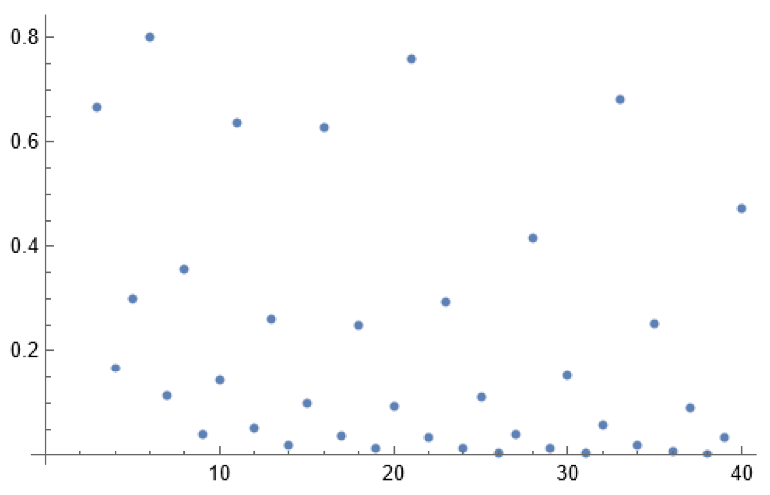
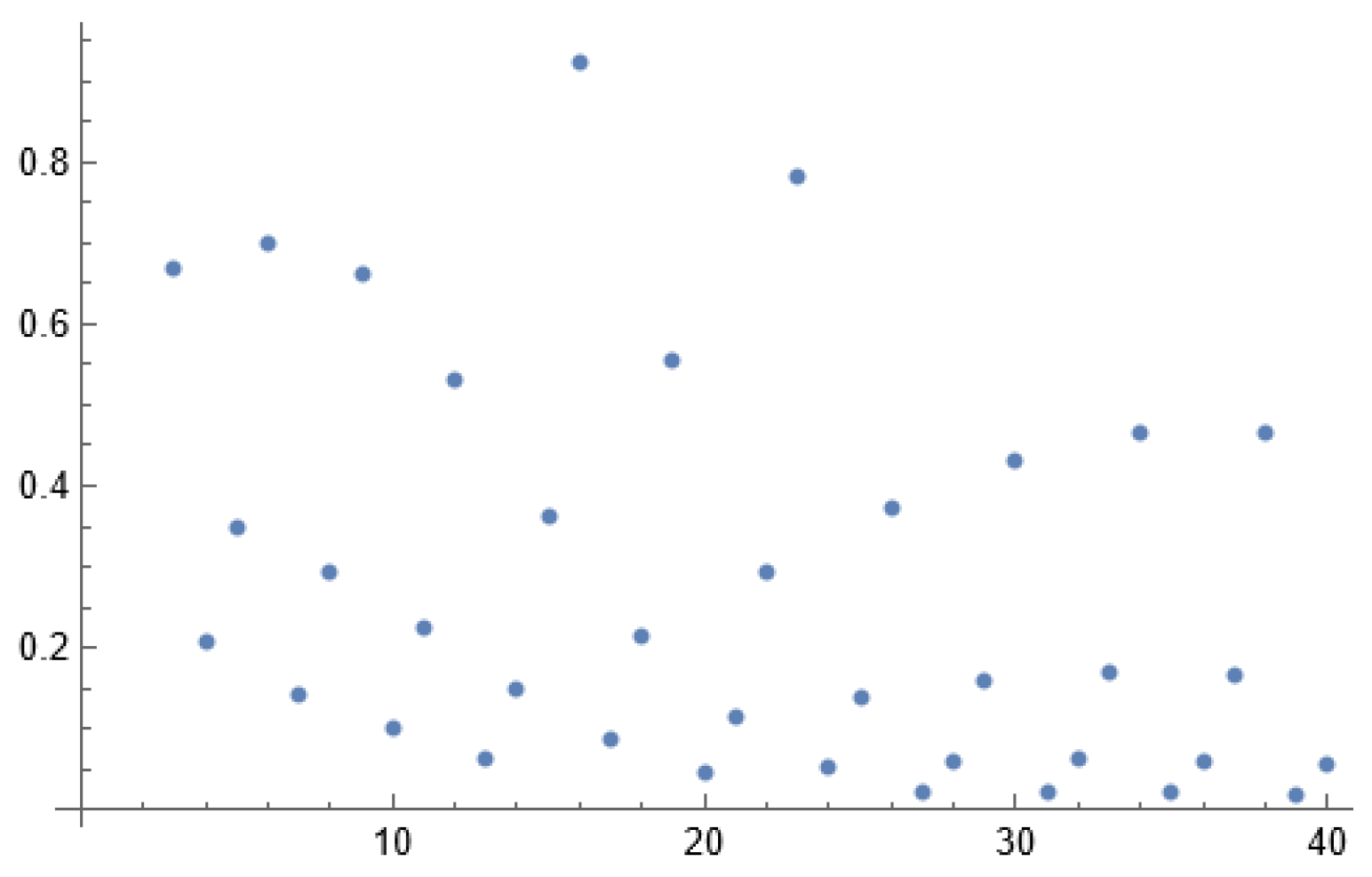
Arrange the points in $S_{1,r}$ from least to greatest and take the 2-d Euclidean distance between each pair of consecutive points in $S_{1,r}$. In this case, since all points lie on $y=1$, take the absolute difference between the x-coordinates of $S_{1,r}$ then call this ${\mathcal{D}}_{1,r}$. (Note, this is similar to $\S$5.3.1 step 3a).

(3)

Repeat step (2) for $S_{2,r}$, then call this ${\mathcal{D}}_{2,r}$. (Note, all point of $S_{2,r}$ lie on $y=0$.)

(4)

Remove any outliers from ${\mathcal{D}}_r={\mathcal{D}}_{1,r}\cup {\mathcal{D}}_{2,r}\cup \left\{d(({\displaystyle \frac{n!-1}{n!}},1),(1,0))\right\}$ (i.e., d is the 2-d Euclidean distance between points $({\displaystyle \frac{n!-1}{n!}},1)$ and $(1,0)$). Note, in this case, ${\mathcal{D}}_{2,r}$ and $\left\{d(({\displaystyle \frac{n!-1}{n!}},1),(1,0))\right\}$ should be outliers (i.e., for any $C>0$, the lengths of ${\mathcal{D}}_{2,r}$ are more than C times the interquartile range of the lengths of ${\mathcal{D}}_r$) leaving us with ${\mathcal{D}}_{1,r}$.

(5)

Multiply the remaining lengths in the pathway by a constant so they add up to one. (See P[r] of code 1 for an example)

(6)

Take the entropy of the probability distribution. (See entropy[r] of code 1 for an example.)

We can illustrate this process with the following code:

Code 1: Illustration of step (1)-(6)

Clear["*Global`*"] A[r_] := A[r] = Range[0, r!]/(r!) (*Below is step 1*) S1[r_] :=  S1[r] = Sort[Select[A[r], Boole[IntegerQ[Denominator[#]/2]] == 1 &]] S2[r_] :=  S2[r] = Sort[Select[A[r], Boole[IntegerQ[Denominator[#]/2]] == 0 &]] (*Below is step 2*) Dist1[r_] := Dist1[r] = Differences[S1[r]] (*Below is step 3*) Dist2[r_] := Dist2[r] = Differences[S2[r]] (*Below is step 4*) NonOutliers[r_] :=  NonOutliers[r] = Dist1[r] (*We exclude Dist2[r] since it’s an outlier*) (*Below is step 5*) P[r_] := P[r] = NonOutliers[r]/Total[NonOutliers[r]] (*Below is step 6*) entropy[r_] := entropy[r] = Total[-P[r] Log[2, P[r]]]

Taking Table[{r,entropy[r]},{r,3,8}], we get:

Code 2: Output of Table[{r,entropy[r]},{r,3,8}]

Clear["*Global`*"] {{{3,1}, {4,(2 Log[11])/(11 Log[2]) + (9 Log[22])/(11 Log[2])},  {5,(14 Log[59])/(59 Log[2]) + (45 Log[118])/(59 Log[2])},  {6,(44 Log[359])/(359 Log[2]) + (315 Log[718])/(359 Log[2])},  {7,(314 Log[2519])/(2519 Log[2]) + (2205 Log[5038])/(2519 Log[2])},  {8,(314 Log[20159])/(20159 Log[2]) + (19845 Log[40318])/(20159 Log[2])}}}

and notice when:

(1)

$c\left(r\right)=(r!)/2-1$

(2)

$\left\{b\left(4\right)\mapsto 9,b\left(5\right)\mapsto 45,b\left(6\right)\mapsto 315,b\left(7\right)\mapsto 2205,b\left(8\right)\mapsto 19845\right\}$

(3)

$a\left(r\right)+b\left(r\right)=c\left(r\right)$

the output of code can be defined:

$${\displaystyle \frac{a\left(r\right){log}_2\left(c\left(r\right)\right)}{c\left(r\right)}}+{\displaystyle \frac{b\left(r\right)log\left(2c\right(r\left)\right)}{c\left(r\right)}}={\displaystyle \frac{a\left(r\right){log}_2\left(c\left(r\right)\right)+b\left(r\right)log\left(2c\left(r\right)\right)}{c\left(r\right)}}$$

(36)

Hence, since $a\left(r\right)=c\left(r\right)-b\left(r\right)=(r!)/2-1-b\left(r\right)$:

$$\begin{array}{cc}\hfill & {\displaystyle \frac{a\left(r\right){log}_2\left(c\left(r\right)\right)+b\left(r\right)log\left(2c\left(r\right)\right)}{c\left(r\right)}}=\hfill \end{array}$$

(37)

$$\begin{array}{cc}\hfill & {\displaystyle \frac{(r!/2-1-b\left(r\right)){log}_2\left(c\left(r\right)\right)+b\left(r\right){log}_2\left(2c\left(r\right)\right)}{c\left(r\right)}}=\hfill \end{array}$$

(38)

$$\begin{array}{cc}\hfill & {\displaystyle \frac{(r!/2){log}_2\left(c\left(r\right)\right)-{log}_2\left(c\left(r\right)\right)-b\left(r\right){log}_2\left(r\right)+b\left(r\right){log}_2\left(c\left(r\right)\right)+b\left(r\right){log}_2\left(2\right)}{c\left(r\right)}}=\hfill \end{array}$$

(39)

$$\begin{array}{cc}\hfill & {\displaystyle \frac{(r!/2){log}_2\left(c\left(r\right)\right)-{log}_2\left(c\left(r\right)\right)+b\left(r\right)}{c\left(r\right)}}=\hfill \end{array}$$

(40)

$$\begin{array}{cc}\hfill & {\displaystyle \frac{(r!/2-1){log}_2\left(c\left(r\right)\right)+b\left(r\right)}{c\left(r\right)}}=\hfill \end{array}$$

(41)

$$\begin{array}{cc}\hfill & {\displaystyle \frac{(r!/2-1){log}_2(r!/2-1)+b\left(r\right)}{r!/2-1}}=\hfill \end{array}$$

(42)

$$\begin{array}{cc}\hfill & {log}_2(r!/2-1)+{\displaystyle \frac{b\left(r\right)}{r!/2-1}}=\hfill \end{array}$$

(43)

and ${lim}_{r\to \infty }b\left(r\right)/c\left(r\right)=1$ (I need help proving this):

$$\begin{array}{cc}\hfill & {log}_2(r!/2-1)+{\displaystyle \frac{b\left(r\right)}{r!/2-1}}\sim {log}_2(r!/2-1)+1\hfill \end{array}$$

(44)

$$\begin{array}{cc}\hfill & {log}_2(r!/2-1)+{log}_2\left(2\right)=\hfill \end{array}$$

(45)

$$\begin{array}{cc}\hfill & {log}_2\left(2(r!/2-1)\right)\hfill \end{array}$$

(46)

$$\begin{array}{cc}\hfill & {log}_2(r!-2)\sim {log}_2(r!)\hfill \end{array}$$

(47)

Hence, entropy[r] is the same as:

$$\begin{array}{cc}\hfill & \mathrm{E}\left(\mathcal{L}\left(\mathcal{S}(\mathbf{C}(1,G_r^{★},\omega ),\psi )\right)\right)\sim {log}_2(r!)\hfill \end{array}$$

(48)

Now, repeat code with:

$${\left(A_j^{★★}\right)}_{j\in \mathbb{N}}=\left(\left\{c/d:c\in \mathbb{Z},d\in \mathbb{N},d\le j,0\le c\le j\right\}\right)$$

Code 3: Illustration of step (1)-(6) on $\left(A_j^{★★}\right)$

Clear["*Global`*"] A[j_] := A[j] =   DeleteDuplicates[Flatten[Table[Range[0, t]/t, {t, 1, j}]]] (*Below is step 1*) S1[j_] :=  S1[j] = Sort[Select[A[j], Boole[IntegerQ[Denominator[#]/2]] == 1 &]] S2[j_] :=  S2[j] = Sort[Select[A[j], Boole[IntegerQ[Denominator[#]/2]] == 0 &]] (*Below is step 2*) Dist1[j_] := Dist1[j] = Differences[S1[j]] (*Below is step 3*) Dist2[j_] := Dist2[j] = Differences[S2[j]] (*Below is step 4*) NonOutliers[j_] :=  NonOutliers[j] = Join[Dist1[j], Dist2[j]] (*There are no outliers*) (*Below is step 5*) P[j_] := P[j] = NonOutliers[j]/Total[NonOutliers[j]] (*Below is step 6*) entropy[j_] := entropy[j] = N[Total[-P[j] Log[2, P[j]]]]

Using this post [21], we assume an approximation of Table[entropy[j],{j,3,Infinity}] or

$\mathrm{E}\left(\mathcal{L}\left(\mathcal{S}(\mathbf{C}(1,G_j^{★★},{\omega }^{\prime }),{\psi }^{\prime })\right)\right)$ is:

$$\begin{array}{cc}\hfill & \mathrm{E}\left(\mathcal{L}\left(\mathcal{S}(\mathbf{C}(1,G_j^{★★},{\omega }^{\prime }),{\psi }^{\prime })\right)\right)\sim 2{log}_2\left(j\right)+1-{log}_2\left(3\pi \right)\hfill \end{array}$$

(49)

Hence, using §5.3.2 (a) and §5.3.2 (1), take $\left|\mathcal{S}(\mathbf{C}(\epsilon ,G_j^{★★},{\omega }^{\prime }),{\psi }^{\prime })\right|={\sum }_{M=1}^j\varphi \left(M\right)\approx {\displaystyle \frac{3}{{\pi }^2}}{j}^2$ (where $\varphi$ is Euler’s Totient function) computing the following:

$$\begin{array}{cc}& \underline{\left|\mathcal{S}(\mathbf{C}(\epsilon ,G_r^{★},\omega ),\psi )\right|}=\hfill \\ \hfill & sup\left\{\left|\mathcal{S}(\mathbf{C}(\epsilon ,G_j^{★★},{\omega }^{\prime }),{\psi }^{\prime })\right|:j\in \mathbb{N},{\omega }^{\prime }\in {\Omega }_{\epsilon ,j},{\psi }^{\prime }\in {\Psi }_{\epsilon ,j,\omega },\mathrm{E}\left(\mathcal{L}\left(\mathcal{S}(\mathbf{C}(\epsilon ,G_j^{★★},{\omega }^{\prime }),{\psi }^{\prime })\right)\right)\le \mathrm{E}\left(\mathcal{L}\left(\mathcal{S}(\mathbf{C}(\epsilon ,G_r^{★},\omega ),\psi )\right)\right)\right\}=\hfill \\ \hfill & sup\left\{{\displaystyle \frac{3}{{\pi }^2}}{j}^2:j\in \mathbb{N},{\omega }^{\prime }\in {\Omega }_{\epsilon ,j},{\psi }^{\prime }\in {\Psi }_{\epsilon ,j,\omega },2{log}_2\left(j\right)+1-{log}_2\left(3\pi \right)\le {log}_2(r!)\right\}=\hfill \end{array}$$

(50)

where:

(1)

For every $r\in \mathbb{N}$, we find a $j\in \mathbb{N}$, where $2{log}_2\left(j\right)+1-{log}_2\left(3\pi \right)\le {log}_2(r!)$, but the absolute value of ${log}_2(r!)-\left(2{log}_2\left(j\right)+1-{log}_2\left(3\pi \right)\right)$ is minimized. In other words, for every $r\in \mathbb{N}$, we want $j\in \mathbb{N}$ where:

$$\begin{array}{cc}\hfill & 2{log}_2\left(j\right)+1-{log}_2\left(3\pi \right)\le {log}_2(r!)\hfill \end{array}$$

(51)

$$\begin{array}{cc}\hfill & 2{log}_2\left(j\right)\le {log}_2(r!)-1+{log}_2\left(3\pi \right)\hfill \end{array}$$

(52)

$$\begin{array}{cc}\hfill & {\left(2^{{log}_2\left(j\right)}\right)}^2\le 2^{{log}_2(r!)-1+{log}_2\left(3\pi \right)}\hfill \end{array}$$

(53)

$$\begin{array}{cc}\hfill & j^2\le \left(2^{{log}_2(r!)}{2}^{{log}_2\left(3\pi \right)}\right)/2\hfill \end{array}$$

(54)

$$\begin{array}{cc}\hfill & j\le \sqrt{{\displaystyle \frac{r!\left(3\pi \right)}{2}}}\hfill \end{array}$$

(55)

$$\begin{array}{cc}\hfill & j=⌊\sqrt{{\displaystyle \frac{3\pi r!}{2}}}⌋\hfill \end{array}$$

(56)

$$\begin{array}{cc}\hfill & {\displaystyle \frac{3}{{\pi }^2}}{j}^2={\displaystyle \frac{3}{{\pi }^2}}{\left(⌊\sqrt{{\displaystyle \frac{3\pi r!}{2}}}⌋\right)}^2\sim \underline{\left|\mathcal{S}(\mathbf{C}(1,G_r^{★},\omega ),\psi )\right|}\hfill \end{array}$$

(57)

Finally, since $\left|\mathcal{S}(\mathbf{C}(\epsilon ,G_r^{★},\omega ),\psi )\right|=r!$, we wish to prove

$$1<\underset{\epsilon \to 0}{lim\; inf}\underset{r\to \infty }{lim\; inf}\underset{\omega \in {\Omega }_{\epsilon ,r}}{inf}\underset{\psi \in {\Psi }_{\epsilon ,r,\omega }}{inf}\underline{\alpha }\left(\epsilon ,r,\omega ,\psi \right)<+\infty$$

within §5.3.2 crit. 1:

$$\begin{array}{cc}\hfill & \underset{\epsilon \to 0}{lim\; inf}\underset{r\to \infty }{lim\; inf}\underset{\omega \in {\Omega }_{\epsilon ,r}}{inf}\underset{\psi \in {\Psi }_{\epsilon ,r,\omega }}{inf}\underline{\alpha }\left(\epsilon ,r,\omega ,\psi \right)=\underset{r\to \infty }{lim\; inf}\underset{\omega \in {\Omega }_{\epsilon ,r}}{inf}\underset{\psi \in {\Psi }_{\epsilon ,r,\omega }}{inf}{\displaystyle \frac{\underline{\left|\mathcal{S}(\mathbf{C}(\epsilon ,F_r^{★},\omega ),\psi )\right|}}{\left|\mathcal{S}(\mathbf{C}(1,G_r^{★},\omega ),\psi ))\right|}}\hfill \end{array}$$

(58)

$$\begin{array}{cc}\hfill & =\underset{r\to \infty }{lim}{\displaystyle \frac{\frac{3}{{\pi }^2}{\left(⌊\sqrt{\frac{3\pi r!}{2}}⌋\right)}^2}{r!}}\hfill \end{array}$$

(59)

where using mathematica, we get the limit is greater than one:

Code 4: Limitof eq. 59

Clear["*Global`*"] N[Limit[((3/Pi^2) (Floor[Sqrt[(3 Pi r!)/2]])^2)/(r!), r -> Infinity]]  (*Output is 1.43239*)

Also, using §5.3.2 (b) and §5.3.2 (1), take $\left|\mathcal{S}(\mathbf{C}(\epsilon ,G_j^{★★},{\omega }^{\prime }),{\psi }^{\prime })\right|={\sum }_{M=1}^j\varphi \left(M\right)\approx {\displaystyle \frac{3}{{\pi }^2}}{j}^2$ (where $\varphi$ is Euler’s Totient function) to compute the following:

$$\begin{array}{cc}& \underline{\left|\mathcal{S}(\mathbf{C}(\epsilon ,G_r^{★},\omega ),\psi )\right|}=\hfill \\ \hfill & inf\left\{\left|\mathcal{S}(\mathbf{C}(\epsilon ,G_j^{★★},{\omega }^{\prime }),{\psi }^{\prime })\right|:j\in \mathbb{N},{\omega }^{\prime }\in {\Omega }_{\epsilon ,j},{\psi }^{\prime }\in {\Psi }_{\epsilon ,j,\omega },\mathrm{E}\left(\mathcal{L}\left(\mathcal{S}(\mathbf{C}(\epsilon ,G_j^{★★},{\omega }^{\prime }),{\psi }^{\prime })\right)\right)\ge \mathrm{E}\left(\mathcal{L}\left(\mathcal{S}(\mathbf{C}(\epsilon ,G_r^{★},\omega ),\psi )\right)\right)\right\}=\hfill \\ \hfill & inf\left\{{\displaystyle \frac{3}{{\pi }^2}}{j}^2:j\in \mathbb{N},{\omega }^{\prime }\in {\Omega }_{\epsilon ,j},{\psi }^{\prime }\in {\Psi }_{\epsilon ,j,\omega },2{log}_2\left(j\right)+1-{log}_2\left(3\pi \right)\ge {log}_2(r!)\right\}=\hfill \end{array}$$

(60)

where:

(1)

For every $r\in \mathbb{N}$, we find a $j\in \mathbb{N}$, where $2{log}_2\left(j\right)+1-{log}_2\left(3\pi \right)\ge {log}_2(r!)$, but the absolute value of $\left(2{log}_2\left(j\right)+1-{log}_2\left(3\pi \right)\right)-{log}_2(r!)$ is minimized. In other words,

for every $r\in \mathbb{N}$, we want $j\in \mathbb{N}$ where:

$$\begin{array}{cc}\hfill & 2{log}_2\left(j\right)+1-{log}_2\left(3\pi \right)\ge {log}_2(r!)\hfill \end{array}$$

(61)

$$\begin{array}{cc}\hfill & 2^{2{log}_2\left(j\right)}\ge {log}_2(r!)-1+{log}_2\left(3\pi \right)\hfill \end{array}$$

(62)

$$\begin{array}{cc}\hfill & {\left(2^{{log}_2\left(j\right)}\right)}^2\ge 2^{{log}_2(r!)-1+{log}_2\left(3\pi \right)}\hfill \end{array}$$

(63)

$$\begin{array}{cc}\hfill & j^2\ge \left(2^{{log}_2(r!)}{2}^{{log}_2\left(3\pi \right)}\right)/2\hfill \end{array}$$

(64)

$$\begin{array}{cc}\hfill & j\ge \sqrt{{\displaystyle \frac{r!\left(3\pi \right)}{2}}}\hfill \end{array}$$

(65)

$$\begin{array}{cc}\hfill & j=⌈\sqrt{{\displaystyle \frac{3\pi r!}{2}}}⌉\hfill \end{array}$$

(66)

$$\begin{array}{cc}\hfill & {\displaystyle \frac{3}{{\pi }^2}}{j}^2={\displaystyle \frac{3}{{\pi }^2}}{\left(⌈\sqrt{{\displaystyle \frac{3\pi r!}{2}}}⌉\right)}^2\sim \overline{\left|\mathcal{S}(\mathbf{C}(1,G_r^{★},\omega ),\psi )\right|}\hfill \end{array}$$

(67)

Finally, since $\left|\mathcal{S}(\mathbf{C}(1,G_r^{★},\omega ),\psi )\right|=r!$, we wish to prove

$$1<\underset{\epsilon \to 0}{lim\; sup}\underset{r\to \infty }{lim\; sup}\underset{\omega \in {\Omega }_{\epsilon ,r}}{sup}\underset{\psi \in {\Psi }_{\epsilon ,r,\omega }}{sup}\overline{\alpha }\left(\epsilon ,r,\omega ,\psi \right)<+\infty$$

within §5.3.2 crit. 1:

$$\begin{array}{cc}\hfill & \underset{\epsilon \to 0}{lim\; sup}\underset{r\to \infty }{lim\; sup}\underset{\omega \in {\Omega }_{\epsilon ,r}}{sup}\underset{\psi \in {\Psi }_{\epsilon ,r,\omega }}{sup}\overline{\alpha }\left(\epsilon ,r,\omega ,\psi \right)=\underset{r\to \infty }{lim\; sup}\underset{\omega \in {\Omega }_{\epsilon ,r}}{sup}\underset{\psi \in {\Psi }_{\epsilon ,r,\omega }}{sup}{\displaystyle \frac{\overline{\left|\mathcal{S}(\mathbf{C}(1,G_r^{★},\omega ),\psi )\right|}}{\left|\mathcal{S}(\mathbf{C}(1,G_r^{★},\omega ),\psi ))\right|}}\hfill \end{array}$$

(68)

$$\begin{array}{cc}\hfill & =\underset{r\to \infty }{lim}{\displaystyle \frac{\frac{3}{{\pi }^2}{\left(⌈\sqrt{\frac{3\pi r!}{2}}⌉\right)}^2}{r!}}\hfill \end{array}$$

(69)

where using mathematica, we get the limit is greater than one:

Code 5: Limitof eq. 69

N[Limit[((3/Pi^2) (Ceiling[Sqrt[(3 Pi r!)/2]])^2)/(r!), r -> Infinity]]  (*The output is 1.43239*)

Hence, since the limits in eq. 58 and eq. 68 are greater than one and less than $+\infty$: i.e.,

$$1<\underset{\epsilon \to 0}{lim\; inf}\underset{r\to \infty }{lim\; inf}\underset{\omega \in {\Omega }_{\epsilon ,r}}{inf}\underset{\psi \in {\Psi }_{\epsilon ,r,\omega }}{inf}\underline{\alpha }\left(\epsilon ,r,\omega ,\psi \right)=\underset{\epsilon \to 0}{lim\; sup}\underset{r\to \infty }{lim\; sup}\underset{\omega \in {\Omega }_{\epsilon ,r}}{sup}\underset{\psi \in {\Psi }_{\epsilon ,r,\omega }}{sup}\overline{\alpha }\left(\epsilon ,r,\omega ,\psi \right)<+\infty$$

(70)

what we’re measuring from${\left(G_r^{★}\right)}_{r\in \mathbb{N}}$ increases at a rate superlinear to that of ${\left(G_j^{★★}\right)}_{j\in \mathbb{N}}$ (i.e., 5.3.2 crit. 1).

5.3.4. Example of The “Measure" from ${\left(G_r^{★}\right)}_{r\in \mathbb{N}}$ Increasing at a Rate Sub-Linear to That of ${\left(G_j^{★★}\right)}_{j\in \mathbb{N}}$

Using our previous example, we can use the following theorem:

Theorem 5. 

If what we’re measuring from ${\left(G_r^{★}\right)}_{r\in \mathbb{N}}$ increases at a rate superlinear to that of ${\left(G_j^{★★}\right)}_{j\in \mathbb{N}}$, then what we’re measuring from ${\left(G_j^{★★}\right)}_{r\in \mathbb{N}}$ increases at a ratesublinearto that of ${\left(G_r^{★}\right)}_{r\in \mathbb{N}}$

Hence, in our definition of super-linear (§5.3.2 crit. 2), swap $G_r^{★}$ and $r\in \mathbb{N}$ for $\left(G_j^{★★}\right)$ and $j\in \mathbb{N}$ regarding $\overline{\alpha }\left(ϵ,r,\omega ,\psi \right)$ and $\underline{\alpha }\left(ϵ,r,\omega ,\psi \right)$ (i.e., $\overline{\alpha }\left(ϵ,j,\omega ,\psi \right)$ and $\underline{\alpha }\left(ϵ,j,\omega ,\psi \right)$) and notice thm. 5 is true when:

$$1<\underset{\epsilon \to 0}{lim\; sup}\underset{j\to \infty }{lim\; sup}\underset{\omega \in {\Omega }_{\epsilon ,j}}{sup}\underset{\psi \in {\Psi }_{\epsilon ,j,\omega }}{sup}\overline{\alpha }\left(\epsilon ,j,\omega ,\psi \right),\underset{\epsilon \to 0}{lim\; inf}\underset{j\to \infty }{lim\; inf}\underset{\omega \in {\Omega }_{\epsilon ,j}}{inf}\underset{\psi \in {\Psi }_{\epsilon ,j,\omega }}{inf}\underline{\alpha }\left(\epsilon ,j,\omega ,\psi \right)<+\infty$$

5.3.5. Example of The “Measure" from ${\left(G_r^{★}\right)}_{r\in \mathbb{N}}$ Increasing at a Rate Linear to That of ${\left(G_j^{★★}\right)}_{j\in \mathbb{N}}$

Suppose, we have function $f:A\to \mathbb{R}$, where $A=\mathbb{Q}\cap [0,1]$, and:

$$f\left(x\right)=\left\{\begin{array}{cc}1\hfill & x\in \left\{(2s+1)/\left(2t\right):s\in \mathbb{Z},t\in \mathbb{N},t\ne 0\right\}\cap [0,1]\hfill \\ 0\hfill & x\notin \left\{(2s+1)/\left(2t\right):s\in \mathbb{Z},t\in \mathbb{N},t\ne 0\right\}\cap [0,1]\hfill \end{array}\right.$$

(71)

such that:

$${\left(A_r^{★}\right)}_{r\in \mathbb{N}}={\left(\left\{c/r!:c\in \mathbb{Z},0\le c\le r!\right\}\right)}_{r\in \mathbb{N}}$$

and

$${\left(A_j^{★★}\right)}_{j\in \mathbb{N}}=\left(\left\{c/\left({(j!)}^2\right):c\in \mathbb{N},1\le c\le {(j!)}^2\right\}\right)$$

where for $f_r^{★}:A_r^{★}\to \mathbb{R}$,

$$f_r^{★}\left(x\right)=f\left(x\right)\mathrm{for}\mathrm{all}x\in A_r^{★}$$

(72)

and $f_j^{★★}:A_j^{★★}\to \mathbb{R}$

$$f_j^{★★}\left(x\right)=f\left(x\right)\mathrm{for}\mathrm{all}x\in A_j^{★★}$$

(73)

Hence, when ${\left(G_r^{★}\right)}_{r\in \mathbb{N}}$ is:

$${\left(G_r^{★}\right)}_{r\in \mathbb{N}}={\left(\left\{(x,f\left(x\right)):x\in \left\{c/r!:c\in \mathbb{Z},0\le c\le r!\right\}\right\}\right)}_{r\in \mathbb{N}}$$

(74)

and ${\left(G_j^{★★}\right)}_{j\in \mathbb{N}}$ is:

$${\left(G_j^{★★}\right)}_{j\in \mathbb{N}}={\left(\left\{(x,f\left(x\right)):x\in \left\{c/\left({(j!)}^2\right):c\in \mathbb{Z},0\le c\le {(j!)}^2\right\}\right\}\right)}_{j\in \mathbb{N}}$$

(75)

We already know, using §5.3.3:

$$\mathrm{E}\left(\mathcal{L}\left(\mathcal{S}(\mathbf{C}(1,G_r^{★},\omega ),\psi )\right)\right)\sim {log}_2(r!-2)\sim {log}_2(r!)$$

(76)

Also, using §5.3.3 steps 1-6 on ${\left(A_j^{★★}\right)}_{j\in \mathbb{N}}$:

Code 6: Illustration of step (1)-(6) on $\left(A_j^{★★}\right)$

Clear["*Global`*"] A[j_] := A[j] =  Range[0, 7 (j!)]/(7 (j!)) (*Below is step 1*) S1[j_] :=  S1[j] = Sort[Select[A[j], Boole[IntegerQ[Denominator[#]/2]] == 1 &]] S2[j_] :=  S2[j] = Sort[Select[A[j], Boole[IntegerQ[Denominator[#]/2]] == 0 &]] (*Below is step 2*) Dist1[j_] := Dist1[j] = Differences[S1[j]] (*Below is step 3*) Dist2[j_] := Dist2[j] = Differences[S2[j]] (*Below is step 4*) NonOutliers[j_] :=  NonOutliers[j] = Dist1[j] (*Dist2[j] is an outlier*) (*Below is step 5*) P[j_] := P[j] = NonOutliers[j]/Total[NonOutliers[j]] (*Below is step 6*) entropy[j_] := entropy[j] = N[Total[-P[j] Log[2, P[j]]]] T = Table[{j,entropy[j]},{j,3,6}]

where the output is

Code 7: Output of Code 6

(*@@*)(@@) {{3,(8 Log[17])/(17 Log[2]) + (9 Log[34])/(17 Log[2])},      {4,(8 Log[287])/(287 Log[2]) + (279 Log[574])/(287 Log[2])},      {5,(224 Log[7199])/(7199 Log[2]) + (6975 Log[14398])/(7199 Log[2])},      {6,(2024 Log[259199])/(259199 Log[2]) + (257175 Log[518398])/(259199 Log[2])}}

Notice when:

(1)

$c\left(j\right)={(j!)}^2/2-1$

(2)

$\left\{b\left(4\right)\mapsto 9,b\left(5\right)\mapsto 279,b\left(6\right)\mapsto 6975,b\left(7\right)\mapsto 257175,b\left(8\right)\mapsto 19845\right\}$

(3)

$a\left(j\right)+b\left(j\right)=c\left(j\right)$

the output of code can be defined:

$${\displaystyle \frac{a\left(j\right){log}_2\left(c\left(j\right)\right)}{c\left(j\right)}}+{\displaystyle \frac{b\left(j\right)log\left(2c\right(j\left)\right)}{c\left(j\right)}}={\displaystyle \frac{a\left(j\right){log}_2\left(c\left(j\right)\right)+b\left(j\right)log\left(2c\left(j\right)\right)}{c\left(j\right)}}$$

(77)

Hence, since $a\left(j\right)=c\left(j\right)-b\left(j\right)={(j!)}^2/2-1-b\left(j\right)$:

$$\begin{array}{cc}\hfill & {\displaystyle \frac{a\left(j\right){log}_2\left(c\left(j\right)\right)+b\left(j\right)log\left(2c\left(j\right)\right)}{c\left(j\right)}}=\hfill \end{array}$$

(78)

$$\begin{array}{cc}\hfill & {\displaystyle \frac{({(j!)}^2/2-1-b\left(j\right)){log}_2\left(c\left(j\right)\right)+b\left(j\right){log}_2\left(2c\left(j\right)\right)}{c\left(j\right)}}=\hfill \end{array}$$

(79)

$$\begin{array}{cc}\hfill & {\displaystyle \frac{({(j!)}^2/2){log}_2\left(c\left(j\right)\right)-{log}_2\left(c\left(j\right)\right)-b\left(j\right){log}_2\left(j\right)+b\left(j\right){log}_2\left(c\left(j\right)\right)+b\left(j\right){log}_2\left(2\right)}{c\left(j\right)}}=\hfill \end{array}$$

(80)

$$\begin{array}{cc}\hfill & {\displaystyle \frac{({(j!)}^2/2){log}_2\left(c\left(j\right)\right)-{log}_2\left(c\left(j\right)\right)+b\left(j\right)}{c\left(j\right)}}=\hfill \end{array}$$

(81)

$$\begin{array}{cc}\hfill & {\displaystyle \frac{({(j!)}^2/2-1){log}_2\left(c\left(j\right)\right)+b\left(j\right)}{c\left(j\right)}}=\hfill \end{array}$$

(82)

$$\begin{array}{cc}\hfill & {\displaystyle \frac{({(j!)}^2/2-1){log}_2({(j!)}^2/2-1)+b\left(j\right)}{{(j!)}^2/2-1}}=\hfill \end{array}$$

(83)

$$\begin{array}{cc}\hfill & {log}_2({(j!)}^2/2-1)+{\displaystyle \frac{b\left(j\right)}{{(j!)}^2/2-1}}=\hfill \end{array}$$

(84)

since ${lim}_{r\to \infty }b\left(r\right)/c\left(r\right)=1$ (this is proven in [22]):

$$\begin{array}{cc}\hfill & {log}_2({(j!)}^2/2-1)+{\displaystyle \frac{b\left(j\right)}{{(j!)}^2/2-1}}\sim {log}_2({(j!)}^2/2-1)+1\hfill \end{array}$$

(85)

$$\begin{array}{cc}\hfill & {log}_2({(j!)}^2/2-1)+{log}_2\left(2\right)=\hfill \end{array}$$

(86)

$$\begin{array}{cc}\hfill & {log}_2({(j!)}^2-2))\sim \hfill \end{array}$$

(87)

$$\begin{array}{cc}\hfill & {log}_2\left({(j!)}^2\right)=\hfill \end{array}$$

(88)

$$\begin{array}{cc}\hfill & 2{log}_2(j!)\hfill \end{array}$$

(89)

Hence, entropy[r] is the same as:

$$\begin{array}{cc}\hfill & \mathrm{E}\left(\mathcal{L}\left(\mathcal{S}(\mathbf{C}(1,G_r^{★},\omega ),\psi )\right)\right)\sim \hfill \end{array}$$

(90)

$$\begin{array}{cc}\hfill & 2{log}_2(j!)\hfill \end{array}$$

(91)

Therefore, using §5.3.2 (a) and §5.3.2 (3a), take $\left|\mathcal{S}(\mathbf{C}(\epsilon ,G_j^{★★},{\omega }^{\prime }),{\psi }^{\prime })\right|={(j!)}^2$ to compute the following:

$$\begin{array}{cc}& \underline{\left|\mathcal{S}(\mathbf{C}(\epsilon ,G_r^{★},\omega ),\psi )\right|}=\hfill \\ \hfill & sup\left\{\left|\mathcal{S}(\mathbf{C}(\epsilon ,G_j^{★★},{\omega }^{\prime }),{\psi }^{\prime })\right|:j\in \mathbb{N},{\omega }^{\prime }\in {\Omega }_{\epsilon ,j},{\psi }^{\prime }\in {\Psi }_{\epsilon ,j,\omega },\mathrm{E}\left(\mathcal{L}\left(\mathcal{S}(\mathbf{C}(\epsilon ,G_j^{★★},{\omega }^{\prime }),{\psi }^{\prime })\right)\right)\le \mathrm{E}\left(\mathcal{L}\left(\mathcal{S}(\mathbf{C}(\epsilon ,G_r^{★},\omega ),\psi )\right)\right)\right\}=\hfill \\ \hfill & sup\left\{{(j!)}^2:j\in \mathbb{N},{\omega }^{\prime }\in {\Omega }_{\epsilon ,j},{\psi }^{\prime }\in {\Psi }_{\epsilon ,j,\omega },2{log}_2(j!)\le {log}_2(r!)\right\}=\hfill \end{array}$$

(92)

where:

(1)

For every $r\in \mathbb{N}$, we find a $j\in \mathbb{N}$, where $2{log}_2(j!)\le {log}_2(r!)$, but the absolute value of ${log}_2(r!)-2{log}_2(j!)$ is minimized. In other words, for every $r\in \mathbb{N}$, we want $j\in \mathbb{N}$ where:

$$\begin{array}{cc}\hfill & 2{log}_2(j!)\le {log}_2(r!)\hfill \end{array}$$

(93)

$$\begin{array}{cc}\hfill & 2^{2{log}_2(j!)}\le 2^{{log}_2(r!)}\hfill \end{array}$$

(94)

$$\begin{array}{cc}\hfill & {\left(2^{{log}_2(j!)}\right)}^2\le r!\hfill \end{array}$$

(95)

$$\begin{array}{cc}\hfill & {(j!)}^2\le r!\hfill \end{array}$$

(96)

$$\begin{array}{cc}\hfill & {(j!)}^2=\lfloor r!\rfloor \hfill \end{array}$$

(97)

To solve for j, we try the following code:

Code 8: Code for j in eq. 97

Clear["Global`*"] T1 = Table[    {sol[r_] := sol[r] = Reduce[j > 0 && ((j!)^2) <= r!, j, Integers],     jsolve = Max[j /. Solve[sol[r], {j}, Integers]],     (* Largest j that solves inequality (j!)^2<=r for every r *)     , N[(jsolve!)^2/(r!)]}, {r, 3, 40}]; Tablejsolve =  Table[{T1[[r - 3 + 1, 2]], r}, {r, 3,    40}] (*Takes largest j-values for every r in r!*) loweralphr =  Table[{r, T1[[r - 3 + 1, 4]]}, {r, 3,    40}] (* Takes largest largest j values and corresponding r value*) ListPlot[loweralphr] (*Graph points of upperalph. Notice, the graph has a lower bound of zero.*)

Note, the output is:

Code 9: Output for code 8

Clear["Global`*"] (* Output of Tablejsolve*) {{2, 3}, {2, 4}, {3, 5}, {4, 6}, {4, 7}, {5, 8}, {5, 9}, {6, 10}, {7, 11}, {7, 12},  {8, 13}, {8, 14}, {9, 15}, {10, 16}, {10, 17}, {11, 18}, {11, 19}, {12, 20}, {13, 21},  {13, 22}, {14, 23}, {14, 24}, {15, 25}, {15, 26}, {16, 27}, {17, 28}, {17, 29},  {18, 30}, {18, 31}, {19, 32}, {20, 33}, {20, 34}, {21, 35}, {21, 36}, {22, 37}, {22, 38},  {23, 39}, {24, 40}} (*Output of loweralphr*) {{3, 0.666667}, {4, 0.166667}, {5, 0.3}, {6, 0.8}, {7, 0.114286}, {8, 0.357143}, {9, 0.0396825},  {10, 0.142857}, {11, 0.636364}, {12, 0.0530303}, {13, 0.261072}, {14, 0.018648}, {15, 0.100699},  {16, 0.629371}, {17, 0.0370218}, {18, 0.248869}, {19, 0.0130984}, {20, 0.0943082}, {21, 0.758956},  {22, 0.034498}, {23, 0.293983}, {24, 0.0122493}, {25, 0.110244}, {26, 0.00424014}, {27,0.0402028},  {28, 0.41495}, {29, 0.0143086}, {30, 0.154533}, {31, 0.00498494}, {32, 0.0562364}, {33, 0.681653},  {34, 0.0200486}, {35, 0.252613}, {36, 0.00701702}, {37, 0.0917902}, {38, 0.00241553},  {39, 0.0327645}, {40, 0.471809}}

Figure 1. Plot of loweralphr

Figure 1. Plot of loweralphr

Finally, since the lower bound of loweralphr is zero, we have shown:

$$\underset{\epsilon \to 0}{lim\; inf}\underset{r\to \infty }{lim\; inf}\underset{\omega \in {\Omega }_{\epsilon ,r}}{inf}\underset{\psi \in {\Psi }_{\epsilon ,r,\omega }}{inf}\underline{\alpha }\left(\epsilon ,r,\omega ,\psi \right)=0$$

(98)

Next, using §5.3.2 (b) and §5.3.2 (3b), take $\left|\mathcal{S}(\mathbf{C}(\epsilon ,G_r^{★},{\omega }^{\prime }),{\psi }^{\prime })\right|=r!$ and swap $r\in \mathbb{N}$ and ${\left(G_r^{★}\right)}_{r\in \mathbb{N}}$ with $j\in \mathbb{N}$ and ${\left(G_j^{★★}\right)}_{j\in \mathbb{N}}$, to compute the following:

$$\begin{array}{cc}& \underline{\left|\mathcal{S}(\mathbf{C}(\epsilon ,G_j^{★★},\omega ),\psi )\right|}=\hfill \\ \hfill & inf\left\{\left|\mathcal{S}(\mathbf{C}(\epsilon ,G_r^{★},{\omega }^{\prime }),{\psi }^{\prime })\right|:r\in \mathbb{N},{\omega }^{\prime }\in {\Omega }_{\epsilon ,r},{\psi }^{\prime }\in {\Psi }_{\epsilon ,r,\omega },\mathrm{E}\left(\mathcal{L}\left(\mathcal{S}(\mathbf{C}(\epsilon ,G_r^{★},{\omega }^{\prime }),{\psi }^{\prime })\right)\right)\ge \mathrm{E}\left(\mathcal{L}\left(\mathcal{S}(\mathbf{C}(\epsilon ,G_j^{★★},\omega ),\psi )\right)\right)\right\}=\hfill \\ \hfill & inf\left\{r!:r\in \mathbb{N},{\omega }^{\prime }\in {\Omega }_{\epsilon ,r},{\psi }^{\prime }\in {\Psi }_{\epsilon ,j,\omega },{log}_2(r!)\ge 2{log}_2(j!)\right\}=\hfill \end{array}$$

(99)

where:

(1)

For every $j\in \mathbb{N}$, we find a $r\in \mathbb{N}$, where ${log}_2(r!)\le 2{log}_2(j!)$, but the absolute value of $2{log}_2(j!)-{log}_2(r!)$ is minimized. In other words, for every $j\in \mathbb{N}$, we want $r\in \mathbb{N}$ where:

$$\begin{array}{cc}\hfill & {log}_2(r!)\le 2{log}_2(j!)\hfill \end{array}$$

(100)

$$\begin{array}{cc}\hfill & 2^{{log}_2(r!)}\le 2^{2{log}_2(j!)}\hfill \end{array}$$

(101)

$$\begin{array}{cc}\hfill & r!\le {\left(2^{{log}_2(j!)}\right)}^2\hfill \end{array}$$

(102)

$$\begin{array}{cc}\hfill & r!\le {(j!)}^2\hfill \end{array}$$

(103)

$$\begin{array}{cc}\hfill & r!={(j!)}^2\hfill \end{array}$$

(104)

To solve r, we try the following code:

Code 10: Code for r in eq. 104

Clear["Global`*"] Clear["Global`*"] T2 = Table[    {sol[j_] := sol[j] = Reduce[j > 0 && r! <= (j!)^2, r, Integers],     rsolve = Max[r /. Solve[sol[j], {r}, Integers]],     (* Largest r that solves inequality (r!)<=(j!)^2 for every r *)     , N[(rsolve!)/((j!)^2)]}, {j, 3, 40}]; Tablersolve =  Table[{T2[[j - 3 + 1, 2]], j}, {j, 3,    40}] (*Takes largest r-values for every j in j!*) loweralphj =  Table[{j, T2[[j - 3 + 1, 4]]}, {j, 3,    40}] (* Takes largest largest r values and corresponding j value*) ListPlot[loweralphj](*Graph points of upperalph. Notice, the graph has a upperbound of Infinity *)

Note, the output is:

Code 11: Output for code 10

Clear["Global`*"] (* Output of Tablersolve*) {{4, 3}, {5, 4}, {7, 5}, {9, 6}, {10, 7}, {12, 8}, {14, 9}, {15, 10}, {17, 11}, {19, 12},  {20, 13}, {22, 14}, {24, 15}, {26, 16}, {27, 17}, {29, 18}, {31, 19}, {32, 20}, {34, 21},  {36, 22}, {38, 23}, {39, 24}, {41, 25}, {43, 26}, {44, 27}, {46, 28}, {48, 29}, {50, 30},  {51, 31}, {53, 32}, {55, 33}, {57, 34}, {58, 35}, {60, 36}, {62, 37}, {64, 38}, {65, 39},  {67, 40}} (*Output of loweralphj*) {{3, 0.666667}, {4, 0.166667}, {5, 0.3}, {6, 0.8}, {7, 0.114286}, {8, 0.357143}, {9, 0.0396825},  {10, 0.142857}, {11, 0.636364}, {12, 0.0530303}, {13, 0.261072}, {14, 0.018648}, {15, 0.100699},  {16, 0.629371}, {17, 0.0370218}, {18, 0.248869}, {19, 0.0130984}, {20, 0.0943082}, {21, 0.758956},  {22, 0.034498}, {23, 0.293983}, {24, 0.0122493}, {25, 0.110244}, {26, 0.00424014}, {27,0.0402028},  {28, 0.41495}, {29, 0.0143086}, {30, 0.154533}, {31, 0.00498494}, {32, 0.0562364}, {33, 0.681653},  {34, 0.0200486}, {35, 0.252613}, {36, 0.00701702}, {37, 0.0917902}, {38, 0.00241553},  {39, 0.0327645}, {40, 0.471809}}

Figure 2. Plot of loweralphj

Figure 2. Plot of loweralphj

since the lower bound of loweralphj is zero, we have shown:

$$\underset{\epsilon \to 0}{lim\; inf}\underset{j\to \infty }{lim\; inf}\underset{\omega \in {\Omega }_{\epsilon ,j}}{inf}\underset{\psi \in {\Psi }_{\epsilon ,j,\omega }}{inf}\underline{\alpha }\left(\epsilon ,j,\omega ,\psi \right)=0$$

(105)

Hence, using eq. 98 and 105, since both:  

(1)

$\underset{\epsilon \to 0}{lim\; sup}\underset{r\to \infty }{lim\; sup}\underset{\omega \in {\Omega }_{\epsilon ,r}}{sup}\underset{\psi \in {\Psi }_{\epsilon ,r,\omega }}{sup}\overline{\alpha }\left(\epsilon ,r,\omega ,\psi \right)$ or $\underset{\epsilon \to 0}{lim\; inf}\underset{r\to \infty }{lim\; inf}\underset{\omega \in {\Omega }_{\epsilon ,r}}{inf}\underset{\psi \in {\Psi }_{\epsilon ,r,\omega }}{inf}\underline{\alpha }\left(\epsilon ,r,\omega ,\psi \right)$ are equal to zero, one or $+\infty$

(2)

$\underset{\epsilon \to 0}{lim\; sup}\underset{j\to \infty }{lim\; sup}\underset{\omega \in {\Omega }_{\epsilon ,j}}{sup}\underset{\psi \in {\Psi }_{\epsilon ,j,\omega }}{sup}\overline{\alpha }\left(\epsilon ,j,\omega ,\psi \right)$ or $\underset{\epsilon \to 0}{lim\; inf}\underset{j\to \infty }{lim\; inf}\underset{\omega \in {\Omega }_{\epsilon ,j}}{inf}\underset{\psi \in {\Psi }_{\epsilon ,j,\omega }}{inf}\underline{\alpha }\left(\epsilon ,j,\omega ,\psi \right)$ are equal to zero, one or $+\infty$

then what I’m measuring from ${\left(G_r^{★}\right)}_{r\in \mathbb{N}}$ increases at a rate linear to that of ${\left(G_j^{★★}\right)}_{j\in \mathbb{N}}$.

5.4. Defining the Actual Rate of Expansion of Sequence of Bounded Sets

5.4.1. Definition of Actual Rate of Expansion of Sequence of Bounded Sets

Suppose ${\left(f_r\right)}_{r\in \mathbb{N}}$ is a sequence of bounded functions converging to f, where ${\left(G_r\right)}_{r\in \mathbb{N}}$ is a sequence of the graph on each $f_r$, and $d(Q,R)$ is the Euclidean distance between points $Q,R\in {\mathbb{R}}^n$. Therefore, using the “chosen" center point $C\in {\mathbb{R}}^{n+1}$, when:

$$\mathcal{G}(C,G_r)=sup\left\{d(C,y):y\in G_r\right\}$$

the actual rate of expansion is:

$$\mathcal{E}(C,G_r)=\mathcal{G}(C,G_{r+1})-\mathcal{G}(C,G_r)$$

Note, there are cases of ${\left(G_r\right)}_{r\in \mathbb{N}}$ when $\mathcal{E}$ isn’t fixed and $\mathcal{E}\ne E$ (i.e., the chosen, fixed rate of expansion).

5.4.2. Example

Suppose, we have $f:A\to \mathbb{R}$, where $A=\mathbb{R}$ and $f\left(x\right)=x$, such that ${\left(A_r^{★}\right)}_{r\in \mathbb{N}}={\left([-r,r]\right)}_{r\in \mathbb{N}}$ and for $f_r^{★}:A_r^{★}\to \mathbb{R}$:

$$f_r^{★}\left(x\right)=f\left(x\right)\mathrm{for}\mathrm{all}x\in A_r^{★}$$

Hence, when ${\left(G_r^{★}\right)}_{r\in \mathbb{N}}$ is:

$${\left(G_r^{★}\right)}_{r\in \mathbb{N}}={\left(\left\{(x,x):x\in [-r,r]\right\}\right)}_{r\in \mathbb{N}}$$

such that $C=(0,0)$, note the farthest point of $G_r^{★}$ from C is either $(-r,-r)$ or $(r,r)$. Hence, to compute $\mathcal{G}(C,G_r^{★})$, we can take $d\left(\right(0,0),(r,r\left)\right)$ or $d\left(\right(0,0),(-r,r\left)\right)$:

$$\begin{array}{cc}\hfill \mathcal{G}(C,G_r^{★})=& sup\left\{d(C,y):y\in G_r^{★}\right\}=\hfill \end{array}$$

(106)

$$\begin{array}{cc}\hfill & d\left(\right(0,0),(r,r\left)\right)=\hfill \end{array}$$

(107)

$$\begin{array}{cc}\hfill & \sqrt{{(0-r)}^2+{(0-r)}^2}=\hfill \end{array}$$

(108)

$$\begin{array}{cc}\hfill & \sqrt{r^2+r^2}=\hfill \end{array}$$

(109)

$$\begin{array}{cc}\hfill & \sqrt{2r^2}=\hfill \end{array}$$

(110)

$$\begin{array}{cc}\hfill & \sqrt{2r^2}=\hfill \end{array}$$

(111)

$$\begin{array}{cc}\hfill & \sqrt{2}\left|r\right|\hfill \end{array}$$

(112)

$$\begin{array}{cc}\hfill & \sqrt{2}r\sin \mathrm{ce}r>0\hfill \end{array}$$

(113)

and the actual rate of expansion is:

$$\begin{array}{cc}\hfill \mathcal{E}(C,G_r^{★})=& \mathcal{G}(C,G_{r+1}^{★})-\mathcal{G}(C,G_r^{★})=\hfill \end{array}$$

(114)

$$\begin{array}{cc}\hfill & \sqrt{2}(r+1)-\sqrt{2}r=\hfill \end{array}$$

(115)

$$\begin{array}{cc}\hfill & \sqrt{2}(r+1)-\sqrt{2}r=\hfill \end{array}$$

(116)

$$\begin{array}{cc}\hfill & \sqrt{2}r+\sqrt{2}-\sqrt{2}r=\hfill \end{array}$$

(117)

$$\begin{array}{cc}\hfill & \sqrt{2}\hfill \end{array}$$

(118)

5.5. Reminder

See if §3.1 is easier to understand.

6. My Attempt at Answering the Blockquote of §1.3.2

6.1. Choice Function

Suppose we define the following:

(1)

${\left(f_k^{★★★}\right)}_{k\in \mathbb{N}}$ is the sequence of bounded functions which satisfies (1), (2), (3), (4) and (5) of the leading question in $\S$3.1

(2)

${\mathbb{S}}^{\prime }\left(f\right)$ is all sequences of bounded functions satisfying (1) of the leading question where the expected values, defined in the papers of $\S$2, is finite.

(3)

${\left(f_j^{★★}\right)}_{j\in \mathbb{N}}$ is an element ${\mathbb{S}}^{\prime }\left(f\right)$ but not an element in the set of sequences of bounded functions to that of ${\left(f_k^{★★★}\right)}_{k\in \mathbb{N}}$ which have equal expected values: i.e., $\sim \left(f_k^{★★★}\right)$. We represent this criteria as:

$${\left(f_j^{★★}\right)}_{j\in \mathbb{N}}\in {\mathbb{S}}^{\prime }\left(f\right)\setminus \sim {\left(f_k^{★★★}\right)}_{k\in \mathbb{N}}$$

Further note, from §5.3.2 (b), if we take:

$$\begin{array}{cc}& \overline{\left|\mathcal{S}(\mathbf{C}(\epsilon ,G_k^{★★★},\omega ),\psi )\right|}=\hfill \\ & inf\left\{\left|\mathcal{S}(\mathbf{C}(\epsilon ,G_j^{★★},{\omega }^{\prime }),{\psi }^{\prime })\right|:j\in \mathbb{N},{\omega }^{\prime }\in {\Omega }_{\epsilon ,j},{\psi }^{\prime }\in {\Psi }_{\epsilon ,j,\omega },\mathrm{E}\left(\mathcal{L}\left(\mathcal{S}(\mathbf{C}(\epsilon ,G_j^{★★},{\omega }^{\prime }),{\psi }^{\prime })\right)\right)\ge \mathrm{E}\left(\mathcal{L}\left(\mathcal{S}(\mathbf{C}(\epsilon ,G_k^{★★★},\omega ),\psi )\right)\right)\right\}\hfill \end{array}$$

(119)

and from §5.3.2 (a), we take:

$$\begin{array}{cc}& \underline{\left|\mathcal{S}(\mathbf{C}(\epsilon ,G_k^{★★★},\omega ),\psi )\right|}=\hfill \\ \hfill & sup\left\{\left|\mathcal{S}(\mathbf{C}(\epsilon ,G_j^{★★},{\omega }^{\prime }),{\psi }^{\prime })\right|:j\in \mathbb{N},{\omega }^{\prime }\in {\Omega }_{\epsilon ,j},{\psi }^{\prime }\in {\Psi }_{\epsilon ,j,\omega },\mathrm{E}\left(\mathcal{L}\left(\mathcal{S}(\mathbf{C}(\epsilon ,G_j^{★★},{\omega }^{\prime }),{\psi }^{\prime })\right)\right)\le \mathrm{E}\left(\mathcal{L}\left(\mathcal{S}(\mathbf{C}(\epsilon ,G_k^{★★★},\omega ),\psi )\right)\right)\right\}\hfill \end{array}$$

(120)

Then, §5.3.1 (2), eq. 119, and eq. 120 is:

$$\begin{array}{c}\underset{\omega \in {\Omega }_{\epsilon ,k}}{sup}\underset{\psi \in {\Psi }_{\epsilon ,k,\omega }}{sup}\left|\mathcal{S}(\mathbf{C}(\epsilon ,G_k^{★★★},\omega ),\psi )\right|=\left|{\mathcal{S}}^{\prime }(\epsilon ,G_k^{★★★})\right|=\left|{\mathcal{S}}^{\prime }\right|\end{array}$$

(121)

$$\begin{array}{c}\underset{\omega \in {\Omega }_{\epsilon ,k}}{sup}\underset{\psi \in {\Psi }_{\epsilon ,k,\omega }}{sup}\overline{\left|\mathcal{S}(\mathbf{C}(\epsilon ,G_k^{★★★},\omega ),\psi )\right|}=\overline{\left|{\mathcal{S}}^{\prime }(\epsilon ,G_k^{★★★})\right|}=\overline{\left|{\mathcal{S}}^{\prime }\right|}\end{array}$$

(122)

$$\begin{array}{c}\underset{\omega \in {\Omega }_{\epsilon ,k}}{sup}\underset{\psi \in {\Psi }_{\epsilon ,k,\omega }}{sup}\underline{\left|\mathcal{S}(\mathbf{C}(\epsilon ,G_k^{★★★},\omega ),\psi )\right|}=\underline{\left|{\mathcal{S}}^{\prime }(\epsilon ,G_k^{★★★})\right|}=\underline{\left|{\mathcal{S}}^{\prime }\right|}\end{array}$$

(123)

6.2. Approach

We manipulate the definitions of §5.3.2 (a) and §5.3.2 (b) to solve (1), (2), (3), (4) and (5) of the leading question in $\S$3.1

6.3. Potential Answer

6.3.1. Preliminaries (Definition of T in Case of §3.1.1 (5))

When the difference of point $X=(x_1,···,x_n)$ and $Y=(y_1,···,y_n)$ is:

$$X-Y=(x_1-y_1,x_2-y_2,···,x_n-y_n)$$

the average of $G_r^{★}$ for every $r\in \mathbb{N}$ is:

$$\mathrm{Avg}\left(G_r^{★}\right)={\displaystyle \frac{1}{{\mathcal{H}}^{{\dim }_{\mathrm{H}}\left(G_r^{★}\right)}\left(G_r^{★}\right)}}{\int }_{G_r^{★}}(x_1,···,x_n)d{\mathcal{H}}^{{\dim }_{\mathrm{H}}\left(G_r^{★}\right)}$$

(124)

and $d(P,Q)$ is the n-d Euclidean distance between points $P,Q\in {\mathbb{R}}^n$, we define an explicit injective $\mathcal{F}:{\mathbb{R}}^n\to \mathbb{R}$ such that:

(1)

If $d(\mathrm{Avg}\left(G_r^{★}\right),C)<d(\mathrm{Avg}\left(G_j^{★★}\right),C)$, then $\mathcal{F}(\mathrm{Avg}\left(G_r^{★}\right)-C)<\mathcal{F}(\mathrm{Avg}\left(G_j^{★★}\right)-C)$

(2)

If $d(\mathrm{Avg}\left(G_r^{★}\right),C)>d(\mathrm{Avg}\left(G_j^{★★}\right),C)$, then $\mathcal{F}(\mathrm{Avg}\left(G_r^{★}\right)-C)>\mathcal{F}(\mathrm{Avg}\left(G_j^{★★}\right)-C)$

(3)

If $d(\mathrm{Avg}\left(G_r^{★}\right),C)=d(\mathrm{Avg}\left(F_j^{★★}\right),C)$, then $\mathcal{F}(\mathrm{Avg}\left(G_r^{★}\right)-C)\ne \mathcal{F}(\mathrm{Avg}\left(G_j^{★★}\right)-C)$

where using “chosen" center point $C\in {\mathbb{R}}^n$:

$$T(C,G_r^{★})=\mathcal{F}(\mathrm{Avg}\left(G_r^{★}\right)-C)$$

(125)

6.3.2. Question

Does T exist? If so, how do we define it?

Hence, using $\left|{\mathcal{S}}^{\prime }\right|$, $\overline{\left|{\mathcal{S}}^{\prime }\right|}$, $\underline{\left|{\mathcal{S}}^{\prime }\right|}$, E, $\mathcal{E}(C,G_k^{★★★})$ (§5.4), and $T(C,F_k^{★★★})$, such that with the absolute value function $\left|\right|·\left|\right|$, ceiling function $\lceil ·\rceil$, and nearest integer function $\left[·\right]$, we define:

$$\begin{array}{cc}& K(\epsilon ,G_k^{★★★})=\hfill \\ & \left(1+\left|\left|E-\mathcal{E}(C,G_k^{★★★})\right|\right|\right)5\left(5\right|5|{\displaystyle \frac{\left|{\mathcal{S}}^{\prime }\right|\left(1+⌈\frac{\left|{\mathcal{S}}^{\prime }\right|\left(\underline{\left|{\mathcal{S}}^{\prime }\right|}+2\left|{\mathcal{S}}^{\prime }\right|\right)}{\left(\underline{\left|{\mathcal{S}}^{\prime }\right|}+\left|{\mathcal{S}}^{\prime }\right|\right)\left(\underline{\left|{\mathcal{S}}^{\prime }\right|}+\left|{\mathcal{S}}^{\prime }\right|+\overline{\left|{\mathcal{S}}^{\prime }\right|}\right)}⌉\right)\left(1+\left[\underline{\left|{\mathcal{S}}^{\prime }\right|}/\left|{\mathcal{S}}^{\prime }\right|\right]\right)}{\left(1+\left[\left|{\mathcal{S}}^{\prime }\right|/\overline{\left|{\mathcal{S}}^{\prime }\right|}\right]\right)\left(1+\left[\underline{\left|{\mathcal{S}}^{\prime }\right|}/\overline{\left|{\mathcal{S}}^{\prime }\right|}\right]\right)}}-\left|{\mathcal{S}}^{\prime }\right|5\left|5\right|+\left|{\mathcal{S}}^{\prime }\right|5)-T(C,G_k^{★★★})\mathcal{E}(C,G_k^{★★★})\hfill \end{array}$$

(126)

where $\mathcal{E}$, E, and T are “removed" when $\mathcal{E},E=0$, the choice function which answers the leading question in $\S$3.1 could be the following, s.t.we explain the reason behind choosing the choice function in §6.4:

Theorem 6. 

If we define:

$$\mathcal{M}(\epsilon ,G_k^{★★★})=\left|{\mathcal{S}}^{\prime }(\epsilon ,G_k^{★★★})\right|\left(K(\epsilon ,G_k^{★★★})-\left|{\mathcal{S}}^{\prime }(\epsilon ,G_k^{★★★})\right|\right)$$

$$\mathcal{M}(\epsilon ,G_j^{★★})=\left|{\mathcal{S}}^{\prime }(\epsilon ,G_j^{★★})\right|\left(K(\epsilon ,G_j^{★★})-\left|{\mathcal{S}}^{\prime }(\epsilon ,G_j^{★★})\right|\right)$$

where for $\mathcal{M}(\epsilon ,G_k^{★★★})$, we define $\mathcal{M}(\epsilon ,G_k^{★★★})$ to be the same as $\mathcal{M}(\epsilon ,G_j^{★★})$ when swapping “$j\in \mathbb{N}$" with “$k\in \mathbb{N}$" (for eq. 119 & 120) and sets $G_k^{★★★}$ with $G_j^{★★}$ (for eq. 119–126), then for constant $v>0$ and variable $v^{*}>0$, if:

$$\overline{\mathcal{S}}(\epsilon ,k,v^{*},G_j^{★★})=inf\left(\left\{|{\mathcal{S}}^{\prime }(\epsilon ,G_j^{★★})|:j\in \mathbb{N},\mathcal{M}(\epsilon ,G_j^{★★})\ge \mathcal{M}(\epsilon ,G_k^{★★★})\ge v^{*}\right\}\cup \left\{v^{*}\right\}\right)+v$$

(127)

and:

$$\underline{\mathcal{S}}(\epsilon ,k,v^{*},G_j^{★★})=sup\left(\left\{|{\mathcal{S}}^{\prime }(\epsilon ,G_j^{★★})|:j\in \mathbb{N},v^{*}\le \mathcal{M}(\epsilon ,G_j^{★★})\le \mathcal{M}(\epsilon ,G_k^{★★★})\right\}\cup \{-v^{*}\}\right)+v$$

(128)

then for all ${\left(f_j^{★★}\right)}_{j\in \mathbb{N}}\in {\mathbb{S}}^{\prime }\left(f\right)\setminus \sim {\left(f_k^{★★★}\right)}_{k\in \mathbb{N}}$ ($\S$ crit. 3), if:

$$inf\left\{\left|\right|1-c\left|\right|:\forall (ϵ>0)\exists (c>0)\forall (k\in \mathbb{N})\exists (j\in \mathbb{N})\left(\left|\left|{\displaystyle \frac{\left|{\mathcal{S}}^{\prime }(\epsilon ,G_k^{★★★})\right|}{\left|{\mathcal{S}}^{\prime }(\epsilon ,G_j^{★★})\right|}}-c\right|\right|<\epsilon \right)\right\}$$

(129)

where $\lceil ·\rceil$ is the ceiling function, E is the fixed rate of expansion, Γ is the gamma function, n is the dimension of ${\mathbb{R}}^n$, ${\dim }_H\left(G_k^{★★★}\right)$ is the Hausdorff dimension of set $G_k^{★★★}\subseteq {\mathbb{R}}^{n+1}$, and ${\mathbf{A}}_k$ is area of the smallest $(n+1)$-dimensional box that contains $A_k^{★★★}$, then:

$$\begin{array}{cccc}& & & V(\epsilon ,G_k^{★★★},n)=\hfill \\ \hfill & \lceil \hfill & & ({\mathbf{A}}_{\mathbf{k}}^{1-\mathrm{sign}\left(E\right)}(E-\mathrm{sign}\left(E\right)+1)\left({\displaystyle \frac{exp\left(nln\left(\pi \right)/2\right)}{\Gamma (n/2+1)}}\right)\left({k!}^{(n-{\dim }_{\mathrm{H}}\left(G_k^{★★★}\right))}\right)\left(k^{\mathrm{sign}\left(E\right)\left({\dim }_{\mathrm{H}}\left(G_k^{★★★}\right)-\mathrm{sign}\left({\dim }_{\mathrm{H}}\left(G_k^{★★★}\right)\right)+1\right)}\right)+\hfill \\ & & & (1-\mathrm{sign}\left({\dim }_{\mathrm{H}}\left(G_k^{★★★}\right)\right)))/\epsilon \rceil /|{\mathcal{S}}^{\prime }(\epsilon ,G_k^{★★★})|\hfill \end{array}$$

(130)

the choice function is:

$$\begin{array}{cccc}& \underset{\epsilon \to 0}{lim\; sup}\underset{v^{*}\to \infty }{lim}\underset{k\to \infty }{lim\; sup}\hfill & & \left({\displaystyle \frac{\mathrm{sign}\left(\mathcal{M}(\epsilon ,G_k^{★★★})\right)\overline{\mathcal{S}}(\epsilon ,k,v^{*},G_j^{★★})}{|{\mathcal{S}}^{\prime }(\epsilon ,G_k^{★★★})|+v}}-c^{-V(\epsilon ,G_k^{★★★},n)}\right)\hfill \\ & & & \left({\displaystyle \frac{\mathrm{sign}\left(\mathcal{M}(\epsilon ,G_k^{★★★})\right)\underline{\mathcal{S}}(\epsilon ,k,v^{*},G_j^{★★})}{|{\mathcal{S}}^{\prime }(\epsilon ,G_k^{★★★})|+v}}-c^{-V(\epsilon ,G_k^{★★★},n)}\right)=\hfill \end{array}$$

(131)

$$\begin{array}{cccc}& \underset{\epsilon \to 0}{lim\; inf}\underset{v^{*}\to \infty }{lim}\underset{k\to \infty }{lim\; inf}\hfill & & \left({\displaystyle \frac{\mathrm{sign}\left(\mathcal{M}(\epsilon ,G_k^{★★★})\right)\overline{\mathcal{S}}(\epsilon ,k,v^{*},G_j^{★★})}{|{\mathcal{S}}^{\prime }(\epsilon ,G_k^{★★★})|+v}}-c^{-V(\epsilon ,G_k^{★★★},n)}\right)\hfill \\ & & & \left({\displaystyle \frac{\mathrm{sign}\left(\mathcal{M}(\epsilon ,G_k^{★★★})\right)\underline{\mathcal{S}}(\epsilon ,k,v^{*},G_j^{★★})}{|{\mathcal{S}}^{\prime }(\epsilon ,G_k^{★★★})|+v}}-c^{-V(\epsilon ,G_k^{★★★},n)}\right)=0\hfill \end{array}$$

(132)

such that ${\left(G_k^{★★★}\right)}_{k\in \mathbb{N}}$ satisfies eq. 131 & eq. 132. (Note, we want $sup\varnothing =-\infty$, $inf\varnothing =+\infty$, and ${\left(f_k^{★★★}\right)}_{k\in \mathbb{N}}$ to answer the leading question of $\S$3.1) where the answer to the blockquote of $\S$1.3.2 is $\mathbb{E}\left[f_k^{★★★}\right]$ (when it exists).

6.4. Explaining the Choice Function and Evidence the Choice Function Is Credible

Notice, before reading the programming in code 12, without the “c"-terms in eq. 131 and eq. 132:

(1)

The choice function in eq. 131 and eq. 132 is zero, when what I’m measuring from ${\left(G_k^{★★★}\right)}_{k\in \mathbb{N}}$ (§5.3.2 criteria 1) increases at a rate superlinear to that of ${\left(G_j^{★★}\right)}_{j\in \mathbb{N}}$, where $\mathrm{sign}\left(\mathcal{M}(\epsilon ,G_k^{★★★})\right)=0$.

(2)

The choice function in eq. 131 and eq. 132 is zero, when for a given ${\left(G_k^{★★★}\right)}_{k\in \mathbb{N}}$ and ${\left(G_j^{★★}\right)}_{j\in \mathbb{N}}$ there doesn’t exist c where eq. 129 is satisfied or $c=0$.

(3)

When c does exist, suppose:

$$\left\{\mathcal{J}\left(k\right):k\in \mathbb{N},{\displaystyle \frac{|{\mathcal{S}}^{\prime }(\epsilon ,G_k^{★★★})|}{|{\mathcal{S}}^{\prime }(\epsilon ,G_{\mathcal{J}\left(k\right)}^{★★})|}}\approx c\right\}$$

(133)

(a)

When $|{\mathcal{S}}^{\prime }(\epsilon ,G_k^{★★★})|<|{\mathcal{S}}^{\prime }(\epsilon ,G_{\mathcal{J}\left(k\right)}^{★★})|$, then:

$$\begin{array}{cc}\hfill & \underset{\epsilon \to 0}{lim\; sup}\underset{v^{*}\to \infty }{lim}\underset{k\to \infty }{lim\; sup}{\displaystyle \frac{\mathrm{sign}\left(\mathcal{M}(\epsilon ,G_k^{★★★})\right)\overline{\mathcal{S}}(\epsilon ,k,v^{*},G_j^{★★})}{|{\mathcal{S}}^{\prime }(\epsilon ,G_k^{★★★})|+v}}=c\hfill \end{array}$$

(134)

$$\begin{array}{cc}\hfill & \underset{\epsilon \to 0}{lim\; inf}\underset{v^{*}\to \infty }{lim}\underset{k\to \infty }{lim\; inf}{\displaystyle \frac{\mathrm{sign}\left(\mathcal{M}(\epsilon ,G_k^{★★★})\right)\underline{\mathcal{S}}(\epsilon ,k,v^{*},G_j^{★★})}{|{\mathcal{S}}^{\prime }(\epsilon ,G_k^{★★★})|+v}}=0\hfill \end{array}$$

(135)

(b)

When $|{\mathcal{S}}^{\prime }(\epsilon ,G_k^{★★★})|>|{\mathcal{S}}^{\prime }(\epsilon ,G_{\mathcal{J}\left(k\right)}^{★★})|$, then:

$$\begin{array}{cc}\hfill & \underset{\epsilon \to 0}{lim\; sup}\underset{v^{*}\to \infty }{lim}\underset{k\to \infty }{lim\; sup}{\displaystyle \frac{\mathrm{sign}\left(\mathcal{M}(\epsilon ,G_k^{★★★})\right)\overline{\mathcal{S}}(\epsilon ,k,v^{*},G_j^{★★})}{|{\mathcal{S}}^{\prime }(\epsilon ,G_k^{★★★})|+v}}=+\infty \hfill \end{array}$$

(136)

$$\begin{array}{cc}\hfill & \underset{\epsilon \to 0}{lim\; inf}\underset{v^{*}\to \infty }{lim}\underset{k\to \infty }{lim\; inf}{\displaystyle \frac{\mathrm{sign}\left(\mathcal{M}(\epsilon ,G_k^{★★★})\right)\underline{\mathcal{S}}(\epsilon ,k,v^{*},G_j^{★★})}{|{\mathcal{S}}^{\prime }(\epsilon ,G_k^{★★★})|+v}}=1/c\hfill \end{array}$$

(137)

Hence, for each sub-criteria under crit. (3), if we subtract one of their limits by their limit value, then eq. 131 and eq. is zero. (We do this using the “c"-term in eq. 131 and 132). However, when the exponents of the “c"-terms aren’t equal to $-1$, the limits of eq. 131 and 132 aren’t equal to zero. We want this, infact, whenever we swap ${\mathcal{S}}^{\prime }(\epsilon ,G_k^{★★★})$ with ${\mathcal{S}}^{\prime }(\epsilon ,G_j^{★★})$. Moreover, we define function $V(\epsilon ,G_k^{★★★},n)$ (i.e., eq. 130), where:

(3)

(i)

When $S^{\prime }(\epsilon ,G_k^{★★★})\gg \mathrm{Numerator}\left(V(\epsilon ,G_k^{★★★},n)\right)$, then eq. 131 and 132 without the “c"-terms are zero. (The “c"-terms approach zero and still allow eq. 131 and 132 to equal zero.)

(ii)

When $S^{\prime }(\epsilon ,G_k^{★★★})\ll \mathrm{Numerator}\left(V(\epsilon ,G_k^{★★★},n)\right)$, then $\mathrm{sign}\left(\mathcal{M}(\epsilon ,G_k^{★★★})\right)$ is zero which makes eq. 131 and 132 equal zero.

(iii)

Here are some examples of the numerator of $V(\epsilon ,G_k^{★★★},n)$ (eq. 130):

A.

When $E=0$, $n=1$, and ${\dim }_H\left(A\right)=0$, the numerator of $V(\epsilon ,G_k^{★★★},n)$ is $\lceil \left(\mathbf{A}k!+1\right)/\epsilon \rceil$

B.

When $E=z$, $n=1$, and ${\dim }_H\left(A\right)=0$, the numerator of $V(\epsilon ,G_k^{★★★},n)$ is $\lceil \left(2zk·k!+1\right)/\epsilon \rceil$

C.

When $E=0$, $n=z_2$, and ${\dim }_H\left(A\right)=z_2$, the numerator of $V(\epsilon ,G_k^{★★★},n)$ is ceiling of constant $\mathbf{A}$ times the volume of an n-dimensional ball with finite radius: i.e.,

$$⌈{\displaystyle \frac{\mathbf{A}{z}_{1}exp\left(z_{2}ln\left(\pi \right)/2\right)}{\Gamma (z_2/2+1)}}/\epsilon ⌉$$

D.

When $E=z_1$, $n=z_2$, and ${\dim }_H\left(A\right)=z_2$, the numerator of $V(\epsilon ,G_k^{★★★},n)$ is ceiling of the volume of the n-dimensional ball: i.e.,

$$⌈{\displaystyle \frac{z_{1}exp\left(z_{2}ln\left(\pi \right)/2\right)}{\Gamma (z_2/2+1)}}{k}^{z_2}/\epsilon ⌉$$

Now, consider the code for eq. 131 and eq. 132. (Note, the set theoretic limit of $G_k^{★★★}$ is the graph of function $f:A\to \mathbb{R}$.) In this example, $A=\mathbb{Q}\cap [0,1]$, and:

$$f\left(x\right)=\left\{\begin{array}{cc}1\hfill & x\in \left\{(2s+1)/\left(2t\right):s\in \mathbb{Z},t\in \mathbb{N},t\ne 0\right\}\cap [0,1]\hfill \\ 0\hfill & x\notin \left\{(2s+1)/\left(2t\right):s\in \mathbb{Z},t\in \mathbb{N},t\ne 0\right\}\cap [0,1]\hfill \end{array}\right.$$

(138)

such that:

$${\left(A_k^{★★★}\right)}_{r\in \mathbb{N}}={\left(\left\{c/k!:c\in \mathbb{Z},0\le c\le k!\right\}\right)}_{k\in \mathbb{N}}$$

the ceiling function is $\lceil ·\rceil$, and:

$${\left(A_j^{★★}\right)}_{j\in \mathbb{N}}={\left(\left\{c/\lceil j!/3\rceil :c\in \mathbb{Z},0\le c\le \lceil j!/3\rceil \right\}\right)}_{j\in \mathbb{N}}$$

such for $f_k^{★}:A_k^{★★★}\to \mathbb{R}$,

$$f_k^{★★★}\left(x\right)=f\left(x\right)\mathrm{for}\mathrm{all}x\in A_k^{★★★}$$

(139)

and $f_j^{★★}:A_j^{★★}\to \mathbb{R}$

$$f_j^{★★}\left(x\right)=f\left(x\right)\mathrm{for}\mathrm{all}x\in A_j^{★★}$$

(140)

Hence, when ${\left(G_k^{★★★}\right)}_{r\in \mathbb{N}}$ is:

$${\left(G_k^{★★★}\right)}_{k\in \mathbb{N}}={\left(\left\{(x,f\left(x\right)):x\in \left\{c/k!:c\in \mathbb{Z},0\le c\le k!\right\}\right\}\right)}_{k\in \mathbb{N}}$$

(141)

and ${\left(G_j^{★★}\right)}_{j\in \mathbb{N}}$ is:

$${\left(G_j^{★★}\right)}_{j\in \mathbb{N}}={\left(\left\{(x,f\left(x\right)):x\in \left\{c/\lceil j!/3\rceil :c\in \mathbb{Z},0\le c\le \lceil j!/3\rceil \right\}\right\}\right)}_{j\in \mathbb{N}}$$

(142)

Note, the following (we leave this to mathematicians to figure LengthS1, LengthS2, Entropy1 and $\mathtt{Entropy}\mathtt{2}$ for other A and f in code 12).

6.4.1. Evidence With Programming

Code 12: Code for eq. 131 and 132 to eq. 141 and eq. 142

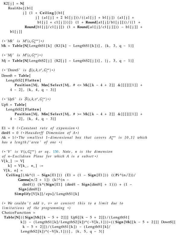
7. Questions

(1)

Does $\S$6 answer the $\mathbf{leading}\mathbf{question}$ in $\S$3.1

(2)

Using thm. 6, when f is defined in $\S$1.1, does $\mathbb{E}\left[f_k^{★★★}\right]$ have a finite value?

(3)

Using thm. 6, when f is defined in $\S$1.2, does $\mathbb{E}\left[f_k^{★★★}\right]$ have a finite value?

(4)

If there’s no time to check questions 1, 2 and 3, see $\S$4.

8.1. Example of §5.3.1, Step 1

Suppose

(1)

$A=\mathbb{R}$

(2)

When defining $f:A\to \mathbb{R}$:

$$f\left(x\right)=\left\{\begin{array}{cc}1\hfill & x<0\hfill \\ -1\hfill & 0\le x<0.5\hfill \\ 0.5\hfill & 0.5\le x\hfill \end{array}\right.$$

(143)

(3)

${\left(G_r^{★}\right)}_{r\in \mathbb{N}}={\left(\left\{(x,f(x\left)\right):-r\le x\le r\right\}\right)}_{r\in \mathbb{N}}$

Then one example of $\mathbf{C}(\sqrt{2}/6,G_1^{★},1)$, using §5.3.1 step 1, (where $G_1^{★}={\left(\left\{(x,f(x\left)\right):-1\le x\le 1\right\}\right)}_{r\in \mathbb{N}}$) is:

$$\begin{array}{cccc}& \{\hfill & & \left\{(x,f\left(x\right)):-1\le x\le {\displaystyle \frac{\sqrt{2}-6}{6}}\right\},\left\{(x,f\left(x\right)):{\displaystyle \frac{\sqrt{2}-6}{6}}\le x\le {\displaystyle \frac{2\sqrt{2}-6}{6}}\right\},\left\{(x,f\left(x\right)):{\displaystyle \frac{2\sqrt{2}-6}{6}}\le x\le {\displaystyle \frac{3\sqrt{2}-6}{6}}\right\}\hfill \\ & & & \left\{(x,f\left(x\right)):{\displaystyle \frac{3\sqrt{2}-6}{6}}\le x\le {\displaystyle \frac{4\sqrt{2}-6}{6}}\right\},\left\{(x,f\left(x\right)):{\displaystyle \frac{4\sqrt{2}-6}{6}}\le x\le {\displaystyle \frac{5\sqrt{2}-6}{6}}\right\},\left\{(x,f\left(x\right)):{\displaystyle \frac{5\sqrt{2}-6}{6}}\le x\le {\displaystyle \frac{6\sqrt{2}-6}{6}}\right\}\hfill \\ & & & \left\{(x,f\left(x\right)):{\displaystyle \frac{6\sqrt{2}-6}{6}}\le x\le {\displaystyle \frac{7\sqrt{2}-6}{6}}\right\},\left\{(x,f\left(x\right)):{\displaystyle \frac{7\sqrt{2}-6}{6}}\le x\le {\displaystyle \frac{8\sqrt{2}-6}{6}}\right\},\left\{(x,f\left(x\right)):{\displaystyle \frac{8\sqrt{2}-6}{6}}\le x\le {\displaystyle \frac{9\sqrt{2}-6}{6}}\right\}\}\hfill \end{array}$$

(144)

Note, the length of each partition is $\sqrt{2}/6$, where the borders could be approximated as:

$$\begin{array}{cccc}& \{\hfill & & \left\{(x,f(x\left)\right):-1\le x\le -.764\right\},\left\{(x,f(x\left)\right):-.764\le x\le -.528\right\},\left\{(x,f(x\left)\right):-.528\le x\le -.293\right\}\hfill \\ & & & \left\{(x,f(x\left)\right):-.293\le x\le -.057\right\},\left\{(x,f(x\left)\right):-.057\le x\le .178\right\},\left\{(x,f(x\left)\right):.178\le x\le .414\right\}\hfill \\ & & & \left\{(x,f(x\left)\right):.414\le x\le .65\right\},\left\{(x,f(x\left)\right):.65\le x\le .886\right\},\left\{(x,f(x\left)\right):.886\le x\le 1.121\right\}\}\hfill \end{array}$$

(145)

which is illustrated using alternating orange/black lines of equal length covering $G_1^{★}$ (i.e., the black vertical lines are the smallest and largest x-cooridinates of $G_1^{★}$).

(Note, the alternating covers in Figure 3 satisfy step (1) of §5.3.1, because the Hausdorff measure in its dimension of the covers is $\sqrt{2}/6$ and there are 9 covers over-covering $G_1^{★}$: i.e.,

Figure 3. The alternating orange & black lines are the “covers" and the vertical lines are the boundaries of $G_1^{★}$.

Figure 3. The alternating orange & black lines are the “covers" and the vertical lines are the boundaries of $G_1^{★}$.

Definition 1 

(Minimum Covers of Measure $\epsilon =\sqrt{2}/6$ covering $G_1^{★}$). We can compute the minimum covers of $\mathbf{C}(\sqrt{2}/6,G_1^{★},1)$, using the formula:

$$\lceil {\mathcal{H}}^{{\dim }_{\mathrm{H}}\left(G_1^{★}\right)}\left(G_1^{★}\right)/(\sqrt{2}/6)\rceil$$

where $\lceil {\mathcal{H}}^{{\dim }_{\mathrm{H}}\left(G_1^{★}\right)}\left(G_1^{★}\right)/(\sqrt{2}/6)\rceil =\lceil \mathrm{Length}\left([-1,1]\right)/(\sqrt{2}/6)\rceil =\lceil 2/(\sqrt{2}/6)\rceil =\lceil 6\sqrt{2}\rceil =\lceil 6\left(1.4\right)\rceil =\lceil 8+.4\rceil =9$).

Note there are other examples of $\mathbf{C}(\sqrt{2}/6,G_1^{★},\omega )$ for different $\omega$. Here is another case:

which can be defined (see eq. 144 for comparison):

$$\begin{array}{cccc}& \{\hfill & & \left\{(x,f\left(x\right)):{\displaystyle \frac{6-9\sqrt{2}}{6}}\le x\le {\displaystyle \frac{6-8\sqrt{2}}{6}}\right\},\left\{(x,f\left(x\right)):{\displaystyle \frac{6-8\sqrt{2}}{6}}\le x\le {\displaystyle \frac{6-7\sqrt{2}}{6}}\right\},\left\{(x,f\left(x\right)):{\displaystyle \frac{6-7\sqrt{2}}{6}}\le x\le {\displaystyle \frac{6-6\sqrt{2}}{6}}\right\}\hfill \\ & & & \left\{(x,f\left(x\right)):{\displaystyle \frac{6-6\sqrt{2}}{6}}\le x\le {\displaystyle \frac{6-5\sqrt{2}}{6}}\right\},\left\{(x,f\left(x\right)):{\displaystyle \frac{6-5\sqrt{2}}{6}}\le x\le {\displaystyle \frac{6-4\sqrt{2}}{6}}\right\},\left\{(x,f\left(x\right)):{\displaystyle \frac{6-4\sqrt{2}}{6}}\le x\le {\displaystyle \frac{6-3\sqrt{2}}{6}}\right\}\hfill \\ & & & \left\{(x,f\left(x\right)):{\displaystyle \frac{6-3\sqrt{2}}{6}}\le x\le {\displaystyle \frac{6-2\sqrt{2}}{6}}\right\},\left\{(x,f\left(x\right)):{\displaystyle \frac{6-2\sqrt{2}}{6}}\le x\le {\displaystyle \frac{6-\sqrt{2}}{6}}\right\},\left\{(x,f\left(x\right)):{\displaystyle \frac{6-\sqrt{2}}{6}}\le x\le 1\right\}\}\hfill \end{array}$$

(146)

In the case of $G_1^{★}$, there are uncountable different covers$\mathbf{C}(\sqrt{2}/6,G_1^{★},\omega )$ which can be used. For instance, when $0\le \alpha \le (12-9\sqrt{2})/6$ (i.e., $\omega =\alpha -(12-9\sqrt{2})/6+1$) consider:

$$\begin{array}{cccc}& \{\hfill & & \left\{(x,f\left(x\right)):\alpha -1+\alpha \le x\le \alpha +{\displaystyle \frac{\sqrt{2}-6}{6}}\right\},\left\{(x,f\left(x\right)):\alpha +{\displaystyle \frac{\sqrt{2}-6}{6}}\le x\le \alpha +{\displaystyle \frac{2\sqrt{2}-6}{6}}\right\},\left\{(x,f\left(x\right)):\alpha +{\displaystyle \frac{2\sqrt{2}-6}{6}}\le x\le \alpha +{\displaystyle \frac{3\sqrt{2}-6}{6}}\right\}\hfill \\ & & & \left\{(x,f\left(x\right)):\alpha +{\displaystyle \frac{3\sqrt{2}-6}{6}}\le x\le \alpha +{\displaystyle \frac{4\sqrt{2}-6}{6}}\right\},\left\{(x,f\left(x\right)):\alpha +{\displaystyle \frac{4\sqrt{2}-6}{6}}\le x\le \alpha +{\displaystyle \frac{5\sqrt{2}-6}{6}}\right\},\hfill \\ & & & \left\{(x,f\left(x\right)):\alpha +{\displaystyle \frac{5\sqrt{2}-6}{6}}\le x\le \alpha +{\displaystyle \frac{6\sqrt{2}-6}{6}}\right\},\left\{(x,f\left(x\right)):\alpha +{\displaystyle \frac{6\sqrt{2}-6}{6}}\le x\le \alpha +{\displaystyle \frac{7\sqrt{2}-6}{6}}\right\}\hfill \\ & & & \left\{(x,f\left(x\right)):\alpha +{\displaystyle \frac{7\sqrt{2}-6}{6}}\le x\le \alpha +{\displaystyle \frac{8\sqrt{2}-6}{6}}\right\},\left\{(x,f\left(x\right)):\alpha +{\displaystyle \frac{8\sqrt{2}-6}{6}}\le x\le \alpha +{\displaystyle \frac{9\sqrt{2}-6}{6}}\right\}\}\hfill \end{array}$$

(147)

When $\alpha =0$ and $\omega =(9\sqrt{2}-6)/6$, we get Figure 4 and when $\alpha =(12-9\sqrt{2})/6$ and $\omega =1$, we get Figure 3

Figure 4. This is similar to Figure 3, except the start-points of the covers are shifted all the way to the left.

Figure 4. This is similar to Figure 3, except the start-points of the covers are shifted all the way to the left.

8.2. Example of §5.3.1, Step 2

. Suppose:

(1)

$A=\mathbb{R}$

(2)

When defining $f:A\to \mathbb{R}$: i.e.,

$$f\left(x\right)=\left\{\begin{array}{cc}1\hfill & x<0\hfill \\ -1\hfill & 0\le x<0.5\hfill \\ 0.5\hfill & 0.5\le x\hfill \end{array}\right.$$

(148)

(3)

${\left(G_r^{★}\right)}_{r\in \mathbb{N}}={\left(\left\{(x,f(x\left)\right):-r\le x\le r\right\}\right)}_{r\in \mathbb{N}}$

(4)

$G_1^{★}=\left\{(x,f(x\left)\right):-1\le x\le 1\right\}$

(5)

$\mathbf{C}(\sqrt{2}/6,G_1^{★},1)$, using eq. 145 and Figure 3, which is approximately

$$\begin{array}{cccc}& \{\hfill & & \left\{(x,f(x\left)\right):-1\le x\le -.764\right\},\left\{(x,f(x\left)\right):-.764\le x\le -.528\right\},\left\{(x,f(x\left)\right):-.528\le x\le -.293\right\}\hfill \\ & & & \left\{(x,f(x\left)\right):-.293\le x\le -.057\right\},\left\{(x,f(x\left)\right):-.057\le x\le .178\right\},\left\{(x,f(x\left)\right):.178\le x\le .414\right\}\hfill \\ & & & \left\{(x,f(x\left)\right):.414\le x\le .65\right\},\left\{(x,f(x\left)\right):.65\le x\le .886\right\},\left\{(x,f(x\left)\right):.886\le x\le 1.121\right\}\}\hfill \end{array}$$

(149)

Then, an example of $\mathcal{S}(\mathbf{C}(\sqrt{2}/6,G_1^{★},1),1)$ is:

$$\left\{\right(-.9,1),(-.65,1),(-.4,1),(-.2,1),(.1,-1),(.3,-1),(.55,.5),(.75,.5),(1,.5\left)\right\}$$

(150)

Below, we illustrate the sample: i.e., the set of all blue points in each orange and black line of $\mathbf{C}(\sqrt{2}/6,G_1^{★},1)$ covering $G_1^{★}$:

Figure 5. The blue points are the “sample points", the alternative black and orange lines are the “covers", and the red lines are the smallest & largest x-coordinates $G_1^{★}$.

Figure 5. The blue points are the “sample points", the alternative black and orange lines are the “covers", and the red lines are the smallest & largest x-coordinates $G_1^{★}$.

Note, there are multiple samples that can be taken, as long as one sample point is taken from each cover in $\mathbf{C}(\sqrt{2}/6,G_1^{★},1)$.

8.3. Example of §5.3.1, Step 3

Suppose

(1)

$A=\mathbb{R}$

(2)

When defining $f:A\to \mathbb{R}$:

$$f\left(x\right)=\left\{\begin{array}{cc}1\hfill & x<0\hfill \\ -1\hfill & 0\le x<0.5\hfill \\ 0.5\hfill & 0.5\le x\hfill \end{array}\right.$$

(151)

(3)

${\left(G_r^{★}\right)}_{r\in \mathbb{N}}={\left(\left\{(x,f(x\left)\right):-r\le x\le r\right\}\right)}_{r\in \mathbb{N}}$

(4)

$G_1^{★}=\left\{(x,f(x\left)\right):-1\le x\le 1\right\}$

(5)

$\mathbf{C}(\sqrt{2}/6,G_1^{★},1)$, using eq. 145 and Figure 3, is approx.

$$\begin{array}{cccc}& \{\hfill & & \left\{(x,f(x\left)\right):-1\le x\le -.764\right\},\left\{(x,f(x\left)\right):-.764\le x\le -.528\right\},\left\{(x,f(x\left)\right):-.528\le x\le -.293\right\}\hfill \\ & & & \left\{(x,f(x\left)\right):-.293\le x\le -.057\right\},\left\{(x,f(x\left)\right):-.057\le x\le .178\right\},\left\{(x,f(x\left)\right):.178\le x\le .414\right\}\hfill \\ & & & \left\{(x,f(x\left)\right):.414\le x\le .65\right\},\left\{(x,f(x\left)\right):.65\le x\le .886\right\},\left\{(x,f(x\left)\right):.886\le x\le 1.121\right\}\}\hfill \end{array}$$

(152)

(6)

$\mathcal{S}(\mathbf{C}(13/6,G_1^{★},1),1)$, using eq. 150, is:

$$\left\{\right(-.9,1),(-.65,1),(-.4,1),(-.2,1),(.1,-1),(.3,-1),(.55,.5),(.75,.5),(1,.5\left)\right\}$$

(153)

Therefore, consider the following process:

8.3.1. Step 3a

If $\mathcal{S}(\mathbf{C}(\sqrt{2}/6,G_1^{★},1),1)$ is:

$$\left\{\right(-.9,1),(-.65,1),(-.4,1),(-.2,1),(.1,-1),(.3,-1),(.55,.5),(.75,.5),(1,.5\left)\right\}$$

(154)

suppose $x_0=(-.9,1)$. Note, the following:

(1)

$x_1=(-.65,1)$ is the next point in the “pathway" since it’s a point in $\mathcal{S}(\mathbf{C}(\sqrt{2}/6,G_1^{★},1),1)$ with the smallest 2-d Euclidean distance to $x_0$ instead of $x_0$.

(2)

$x_2=(-.4,1)$ is the third point since it’s a point in $\mathcal{S}(\mathbf{C}(\sqrt{2}/6,G_1^{★},1),1)$ with the smallest 2-d Euclidean distance to $x_1$ instead of $x_0$ and $x_1$.

(3)

$x_3=(-.2,1)$ is the fourth point since it’s a point in $\mathcal{S}(\mathbf{C}(\sqrt{2}/6,G_1^{★},1),1)$ with the smallest 2-d Euclidean distance to $x_2$ instead of $x_0$, $x_1$, and $x_2$.

(4)

we continue this process, where the “pathway" of $\mathcal{S}(\mathbf{C}(\sqrt{2}/6,G_1^{★},1),1)$ is:

$$(-.9,1)\to (-.65,1)\to (-.4,1)\to (-.2,1)\to (.55,.5)\to (.75,.5)\to (1,.5)\to (.3,-1)\to (.1,-1)$$

(155)

Note 7. 

If more than one point has the minimum 2-d Euclidean distance from $x_0$, $x_1$, $x_2$, etc. take all potential pathways: e.g., using the sample in eq. 154, if $x_0=(-.65,1)$, then since $(-.9,1)$ and $(-.4,1)$ have the smallest Euclidean distance to $(-.65,1)$, taketwopathways:

$$(-.65,1)\to (-.9,1)\to (-.4,1)\to (-.2,1)\to (.55,.5)\to (.75,.5)\to (1,.5)\to (.3,-1)\to (.1,-1)$$

and also:

$$(-.65,1)\to (-.4,1)\to (-.2,1)\to (-.9,1)\to (.55,.5)\to (.75,.5)\to (1,.5)\to (.3,-1)\to (.1,-1)$$

8.3.2. Step 3b

Next, take the length of all line segments in each pathway. In other words, suppose $d(P,Q)$ is the n-th dim.Euclidean distance between points $P,Q\in {\mathbb{R}}^n$. Using the pathway in eq. 155, we want:

$$\begin{array}{cc}\hfill \{& d\left(\right(-.9,1),(-.65,1\left)\right),d\left(\right(-.65,1),(-.4,1\left)\right),d\left(\right(-.4,1),(-.2,1\left)\right),d\left(\right(-.2,1),(.55,.5\left)\right),\hfill \\ & d\left(\right(.55,.5),(.75,.5\left)\right),d\left(\right(.75,.5),(1,.5\left)\right),d\left(\right(1,.5),(.3,-1\left)\right),d\left(\right(.3,-1),(.1,-1\left)\right)\}\hfill \end{array}$$

(156)

Whose distances can be approximated as:

$$\begin{array}{cc}\hfill \{& .25,.25,.2,.901389,.2,.25,1.655295,.2\}\hfill \end{array}$$

Also, we see the outliers [23] are $.901389$ and $1.655295$ (i.e., notice that the outliers are more prominent for $\epsilon \ll \sqrt{2}/6$). Therefore, remove $.901389$ and $1.655295$ from our set of lengths:

$$\begin{array}{cc}\hfill \{& .25,.25,.2,.2,.25,.2\}\hfill \end{array}$$

This is illustrated using:

Figure 6. The black arrows are the “pathways" whose lengths aren’t outliers. The length of the red arrows in the pathway are outliers.

Figure 6. The black arrows are the “pathways" whose lengths aren’t outliers. The length of the red arrows in the pathway are outliers.

Hence, when $x_0=(-.9,1)$, using §5.3.1 step 3b & eq. 154, we note:

$$\mathcal{L}((-.9,1),\mathcal{S}(\mathbf{C}(\sqrt{2}/6,G_1^{★},1),1))=\{.25,.25,.2,.2,.25,.2\}$$

(157)

8.3.3. Step 3c

To convert the set of distances in eq. 157 into a probability distribution, we take:

$$\sum _{x\in \{.25,.25,.2,.2,.25,.2\}}x=.25+.25+.2+.2+.25+.2=1.35$$

(158)

Then divide each element in $\{.25,.25,.2,.2,.25,.2\}$ by 1.35

$$\{.25/(1.35),.25/(1.35),.2/(1.35),.2/(1.35),.25/(1.35),.2/(1.35\left)\right\}$$

which gives us the probability distribution:

$$\{5/27,5/27,4/27,4/27,5/27,4/27\}$$

Hence,

$$\mathbb{P}\left(\mathcal{L}((-.9,1),\mathcal{S}(\mathbf{C}(\sqrt{2}/6,G_1^{★},1),1))\right)=\{5/27,5/27,4/27,4/27,5/27,4/27\}$$

(159)

8.3.4. Step 3d

Take the shannon entropy of eq. 159:

$$\begin{array}{cc}\hfill & \mathrm{E}\left(\mathbb{P}\left(\mathcal{L}((-.9,1),\mathcal{S}(\mathbf{C}(\sqrt{2}/6,G_1^{★},1),1))\right)\right)=\hfill \\ & \sum _{x\in \mathbb{P}\left(\mathcal{L}((-.9,1),\mathcal{S}(\mathbf{C}(\sqrt{2}/6,G_1^{★},1),1))\right)}-x{log}_{2}x=\sum _{x\in \{5/27,5/27,4/27,4/27,5/27,4/27\}}-x{log}_{2}x=\hfill \\ & -(5/27){log}_2(5/27)-(5/27){log}_2(5/27)-(4/27){log}_2(4/27)-(4/27){log}_2(4/27)-(5/27){log}_2(5/27)-(4/27){log}_2(5/27)=\hfill \\ & -(15/27){log}_2(5/27)-(12/27){log}_2(4/27)\approx 2.57604\hfill \end{array}$$

We shorten $\mathrm{E}\left(\mathbb{P}\left(\mathcal{L}((-.9,1),\mathcal{S}(\mathbf{C}(\sqrt{2}/6,G_1^{★},1),1))\right)\right)$ to $\mathrm{E}\left(\mathcal{L}((-.9,1),\mathcal{S}(\mathbf{C}(\sqrt{2}/6,G_1^{★},1),1))\right)$, giving us:

$$\mathrm{E}\left(\mathcal{L}((-.9,1),\mathcal{S}(\mathbf{C}(\sqrt{2}/6,G_1^{★},1),1))\right)\approx 2.57604$$

(160)

8.3.5. Step 3e

Take the entropy, w.r.t all pathways, of the sample:

$$\left\{\right(-.9,1),(-.65,1),(-.4,1),(-.2,1),(.1,-1),(.3,-1),(.55,.5),(.75,.5),(1,.5\left)\right\}$$

(161)

In other words, we’ll compute:

$$\mathrm{E}\left(\mathcal{L}\left(\mathcal{S}(\mathbf{C}(\sqrt{2}/6,G_1^{★},1),1)\right)\right)=\underset{x_0\in \mathcal{S}(\mathbf{C}(\sqrt{2}/6,G_1^{★},1),1)}{sup}\mathrm{E}\left(\mathcal{L}(x_0,\mathcal{S}(\mathbf{C}(\sqrt{2}/6,G_1^{★},1),1))\right)$$

We do this by repeating §8.3.1-§8.3.4 for different $x_0\in \mathcal{S}(\mathbf{C}(\sqrt{2}/6,G_1^{★},1),1)\left)\right)$ (i.e., in the equation with multiple values, see note 7)

$$\begin{array}{cc}\hfill & \mathrm{E}\left(\mathcal{L}((-.9,1),\mathcal{S}(\mathbf{C}(\sqrt{2}/6,G_1^{★},1),1))\right)\approx 2.57604\hfill \end{array}$$

(162)

$$\begin{array}{cc}\hfill & \mathrm{E}\left(\mathcal{L}((-.65,1),\mathcal{S}(\mathbf{C}(\sqrt{2}/6,G_1^{★},1),1))\right)\approx 2.3131,2.377604\hfill \end{array}$$

(163)

$$\begin{array}{cc}\hfill & \mathrm{E}\left(\mathcal{L}((-.4,1),\mathcal{S}(\mathbf{C}(\sqrt{2}/6,G_1^{★},1),1))\right)\approx 2.3131\hfill \end{array}$$

(164)

$$\begin{array}{cc}\hfill & \mathrm{E}\left(\mathcal{L}((-.2,-1),\mathcal{S}(\mathbf{C}(\sqrt{2}/6,G_1^{★},1),1))\right)\approx 2.57604\hfill \end{array}$$

(165)

$$\begin{array}{cc}\hfill & \mathrm{E}\left(\mathcal{L}((-.1,-1),\mathcal{S}(\mathbf{C}(\sqrt{2}/6,G_1^{★},1),1))\right)\approx 1.86094\hfill \end{array}$$

(166)

$$\begin{array}{cc}\hfill & \mathrm{E}\left(\mathcal{L}((-.3,-1),\mathcal{S}(\mathbf{C}(\sqrt{2}/6,G_1^{★},1),1))\right)\approx 1.85289\hfill \end{array}$$

(167)

$$\begin{array}{cc}\hfill & \mathrm{E}\left(\mathcal{L}((.55,.5),\mathcal{S}(\mathbf{C}(\sqrt{2}/6,G_1^{★},1),1))\right)\approx 2.08327\hfill \end{array}$$

(168)

$$\begin{array}{cc}\hfill & \mathrm{E}\left(\mathcal{L}((.75,.5),\mathcal{S}(\mathbf{C}(\sqrt{2}/6,G_1^{★},1),1))\right)\approx 2.31185\hfill \end{array}$$

(169)

$$\begin{array}{cc}\hfill & \mathrm{E}\left(\mathcal{L}((1,.5),\mathcal{S}(\mathbf{C}(\sqrt{2}/6,G_1^{★},1),1))\right)\approx 2.2622\hfill \end{array}$$

(170)

Hence, since the largest value out of eq. 162-170 is $2.57604$:

$$\mathrm{E}\left(\mathcal{L}\left(\mathcal{S}(\mathbf{C}(13/6,G_1^{★},1),1)\right)\right)=\underset{x_0\in \mathcal{S}(\mathbf{C}(\epsilon ,G_1^{★},3),1)}{sup}\mathrm{E}\left(\mathcal{L}(x_0,\mathcal{S}(\mathbf{C}(\epsilon ,G_1^{★},1),1))\right)\approx 2.57604$$

References

- Krishnan, B. Finding a Published Paper Which Meaningfully Averages The Most Pathalogical Functions (V2), 2024. https://www.researchgate.net/publication/384467315_Finding_a_Published_Research_Paper_Which_Meaningfully_Averages_The_Most_Pathalogical_Functions_v2. [CrossRef]
- Bernardi, C.; Rainaldi, C. Everywhere surjections and related topics: Examples and counterexamples. Le Matematiche 2018, 73, 71–88. Available online: https://www.researchgate.net/publication/325625887_Everywhere_surjections_and_related_topics_Examples_and_counterexamples.
- (https://mathoverflow.net/users/87856/arbuja), A. Is there an explicit, everywhere surjective f:R→R whose graph has zero Hausdorff measure in its dimension? MathOverflow, [https://mathoverflow.net/q/476471]. https://mathoverflow.net/q/476471.
- (https://math.stackexchange.com/users/413/jdh), J. Uncountable sets of Hausdorff dimension zero. Mathematics Stack Exchange, [https://math.stackexchange.com/q/73551]. https://math.stackexchange.com/q/73551.
- (https://mathoverflow.net/users/11009/pablo shmerkin), P.S. Hausdorff dimension of R x X. MathOverflow, [https://mathoverflow.net/q/189274]. https://mathoverflow.net/q/189274.
- Xie, T.; Zhou, S. On a class of fractal functions with graph Hausdorff dimension 2. Chaos, Solitons & Fractals 2007, 32, 1625–1630. Available online: https://www.sciencedirect.com/science/article/pii/S0960077906000129. [CrossRef]
- MFH. Prove the following limits of a sequence of sets? Mathchmaticians, 2023. https://matchmaticians.com/questions/hinaeh.
- OEIS Foundation Inc.. A011371. The On-Line Encyclopedia of Integer Sequences, 1999. https://oeis.org/A011371.
- OEIS Foundation Inc.. A099957. The On-Line Encyclopedia of Integer Sequences, 2005. https://oeis.org/A099957.
- OEIS Foundation Inc.. A002088. The On-Line Encyclopedia of Integer Sequences, 1991. https://oeis.org/A002088.
- Ott, W.; Yorke, J.A. Prevelance. Bulletin of the American Mathematical Society 2005, 42, 263–290. Available online: https://www.ams.org/journals/bull/2005-42-03/S0273-0979-05-01060-8/S0273-0979-05-01060-8.pdf. [CrossRef]
- Achour, R.; Li, Z.; Selmi, B.; Wang, T. A multifractal formalism for new general fractal measures. Chaos, Solitons & Fractals 2024, 181, 114655. Available online: https://www.sciencedirect.com/science/article/abs/pii/S0960077924002066.
- Bedford, T.; Fisher, A.M. Analogues of the Lebesgue density theorem for fractal sets of reals and integers. Proceedings of the London Mathematical Society 1992, 3, 95–124. Available online: https://www.ime.usp.br/~afisher/ps/Analogues.pdf. [CrossRef]
- Bedford, T.; Fisher, A.M. Ratio geometry, rigidity and the scenery process for hyperbolic Cantor sets. Ergodic Theory and Dynamical Systems 1997, 17, 531–564. Available online: https://arxiv.org/pdf/math/9405217. [CrossRef]
- Sipser, M. Introduction to the Theory of Computation, 3 ed.; Cengage Learning, 2012; pp. 275–322.
- Krishnan, B. Bharath Krishnan’s ResearchGate Profile. https://www.researchgate.net/profile/Bharath-Krishnan-4.
- Barański, K.; Gutman, Y.; Śpiewak, A. Prediction of dynamical systems from time-delayed measurements with self-intersections. Journal de Mathématiques Pures et Appliquées 2024, 186, 103–149. Available online: https://www.sciencedirect.com/science/article/pii/S0021782424000345. [CrossRef]
- Caetano, A.M.; Chandler-Wilde, S.N.; Gibbs, A.; Hewett, D.P.; Moiola, A. A Hausdorff-measure boundary element method for acoustic scattering by fractal screens. Numerische Mathematik 2024, 156, 463–532. [Google Scholar] [CrossRef]
- (https://math.stackexchange.com/users/5887/sbf), S. Convergence of functions with different domain. Mathematics Stack Exchange, [https://math.stackexchange.com/q/1063261]. https://math.stackexchange.com/q/1063261.
- M., G. Entropy and Information Theory, 2 ed.; Springer New York: New York [America];, 2011; pp. 61–95. https://ee.stanford.edu/~gray/it.pdf. [CrossRef]
- ydd. Finding the asymptotic rate of growth of a table of value? Mathematica Stack Exchange, [https://mathematica.stackexchange.com/a/307050/34171]. https://mathematica.stackexchange.com/a/307050/34171.
- ydd. How to find a closed form for this pattern (if it exists)? Mathematica Stack Exchange, [https://mathematica.stackexchange.com/a/306951/34171]. https://mathematica.stackexchange.com/a/306951/34171.
- John, R. Outlier. https://en.m.wikipedia.org/wiki/Outlier.
Disclaimer/Publisher’s Note: The statements, opinions and data contained in all publications are solely those of the individual author(s) and contributor(s) and not of MDPI and/or the editor(s). MDPI and/or the editor(s) disclaim responsibility for any injury to people or property resulting from any ideas, methods, instructions or products referred to in the content. |
© 2025 by the authors. Licensee MDPI, Basel, Switzerland. This article is an open access article distributed under the terms and conditions of the Creative Commons Attribution (CC BY) license (http://creativecommons.org/licenses/by/4.0/).