Efficient Large-Scale Urban Parking Prediction: Graph Coarsening Based on Real-Time Parking Service Capability

1. Introduction

Urban transportation systems are facing serious challenges due to the continuous increase in the number of vehicles. Recent statistics [1] reveal that vehicle ownership in China escalated to 417 million in 2022, complemented by a striking addition of 34.78 million new registrations within the year. Particularly at the urban scale, as many as 13 cities saw an increase in car ownership by more than 3 million vehicles, including metropolises like Beijing, Shanghai, and Shenzhen. This surge in vehicle numbers not only leads to traffic congestion but also severely exacerbates parking issues. The expansion of urban parking facilities and spaces cannot keep pace with the growth in vehicle numbers, making it exceedingly difficult to find parking in city centers and commercial areas.

To alleviate the parking difficulty issue, urban-level smart parking platforms [2] have emerged. By leveraging cutting-edge technologies such as digital twins, the Internet of Things, and cloud computing [3], these platforms have successfully integrated urban parking facility resources, effectively solving the problem of information asymmetry between users and available parking spaces. Taking the Wuhan smart parking project [4] as an example, by the end of 2022, the platform had integrated more than 4,000 parking lots, including approximately 480,000 parking space data. With its portability, the platform offers convenience to citizens, who can easily check real-time parking availability in different areas through their mobile phones and use services such as parking reservation [5] and parking navigation [6,7,8] to achieve precise parking. In these platforms, the key to providing smart parking services lies in parking prediction technology [9]. Indeed, parking prediction has always been a hot research topic in urban parking technology [10,11]. By effectively predicting the availability of parking spaces in future time periods, it can not only enhance user experience but also improve parking turnover, optimize drivers’ parking behavior, and thereby help to allocate urban parking resources rationally.

Recent studies have framed such parking prediction tasks as spatio-temporal graph modeling problems [12]. On one hand, this is because parking lots are connected through urban road networks, forming unique parking graphs [13], for which graph convolutional networks can be utilized to capture the spatial characteristics of the parking graph [14]. On the other hand, given the tidal characteristics of parking flow, recurrent neural networks can be employed to fit the time series regression of parking data [15]. This approach, which considers both spatial and temporal dependencies, is known as spatio-temporal Graph Convolutional Networks (GCNs).

However, for the vehicle-dense cities mentioned above, with the rapid development of wireless sensors and the widespread use of vehicles [16], a massive influx of real-time parking data continuously flows into urban-level parking platforms. This leads to a dramatic increase in the volume of parking data managed by existing platforms and the coverage range of the parking Internet of Things network [17]. The rapid influx of such information necessitates an unsustainable amount of time to train spatio-temporal GCNs at the required scale for large-scale urban parking prediction.

To reduce the resources and time costs involved in training the aforementioned models, scholars have been dedicated to finding efficient graph dimensionality reduction techniques [18]. Among various studies, graph coarsening [19] stands out as one of the mainstream methods that can achieve this aim. Its core concept involves merging certain nodes within the graph into a hypernode and then using these hypernodes to construct a coarsened graph, thereby enhancing the learning efficiency and scalability of large-scale graphs [20]. However, a prevailing issue is that existing coarsening methods struggle to be directly applied to complex parking scenarios:

1.

The quality of the input graph significantly determines the performance of downstream tasks [21]. For parking graphs, a high-quality parking graph is not only an abstraction of spatial topology but also a adequate representation of parking behavior and decision-making. Neglecting either aspect will limit the understanding of parking scenarios, thereby negatively affecting the effectiveness of subsequent coarsening tasks as well as the accuracy and robustness of prediction tasks.

2.

Most of the existing coarsening methods only consider reducing the size of the graph structure [22], and the node features of the coarsened graph still being obtained by concatenating the original data. This means that the amount of data has not changed. If the model is trained directly based on the coarsened parking graph, the training overhead is not significantly reduced. Moreover, since the coarsened parking graph loses the original topology, the merged data corresponding to the hypernodes also lose their spatial features, leading to a decrease in prediction accuracy.

Graph attention networks (GAT) have attracted much attention in the transportation field [23] over recent years. By selectively focusing on specific nodes and discerning the importance among various nodes, these mechanisms help models to capture deeper hidden information in the traffic scenarios [24], thereby elevating predictive accuracy. The ParkingRank algorithm [25], which assesses the real-time service capability of parking lots using their static attributes, has been widely applied in parking recommendations [26], parking guidance [2], and other related tasks. We posit that this methodology can be interpreted as a preference-based attention mechanism, adept at capturing the service capability variations across different parking lots by evaluating their significance. This nuanced attention mechanism, by thoroughly considering node characteristics alongside topological connections, offers enriched guidance for the coarsening process, enhancing the model’s overall utility and effectiveness.

Meanwhile, autoencoders (AEs) have been widely used in traffic data compression and reconstruction tasks due to their theoretical ability to achieve lossless compression [27]. Specifically, the encoding module is able to learn the high-dimensional sparse information in traffic data and successfully encode it into a low-dimensional dense tensor [28] for more efficient traffic prediction, while the decoding module is tasked with reconstructing the condensed representations back to their original data form [29]. In this framework, we argue that the introduction of an AE can compensate for the lack of compression of node features in the graph coarsening process. Through the synergy of the encoding and decoding modules, a unified dimensionality reduction of the parking graph structure and features can be achieved, thus providing a more efficient and accurate data representation for the downstream parking prediction task. In summary, the main contributions of this paper can be summarized as follows:

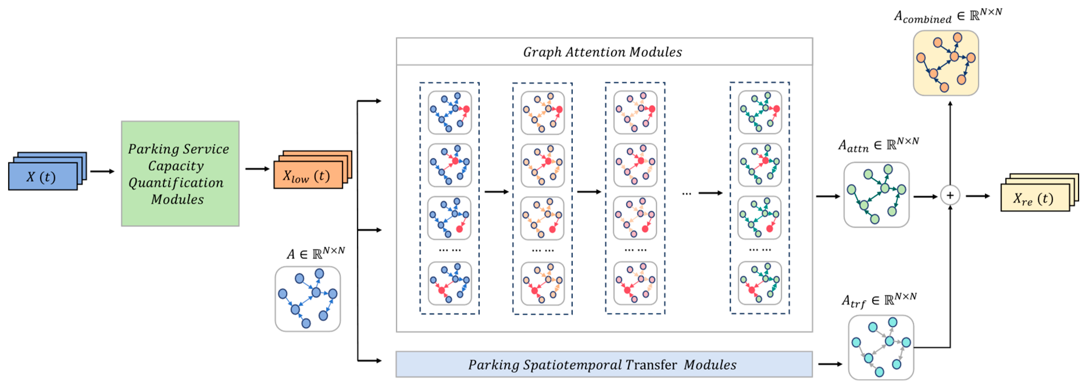
• We have proposed a method for constructing parking graphs that leverages a ParkingRank graph attention mechanism. This method intricately integrates the real-time service capacity assessment of parking lots into a graph attention network, creating a parking graph that accurately mirrors real-world parking behavior preferences. This graph is adept at capturing the complexity of parking scenarios, while also remaining flexible enough to adapt to its dynamic shifts, laying the foundation for downstream coarsening as well as prediction tasks.
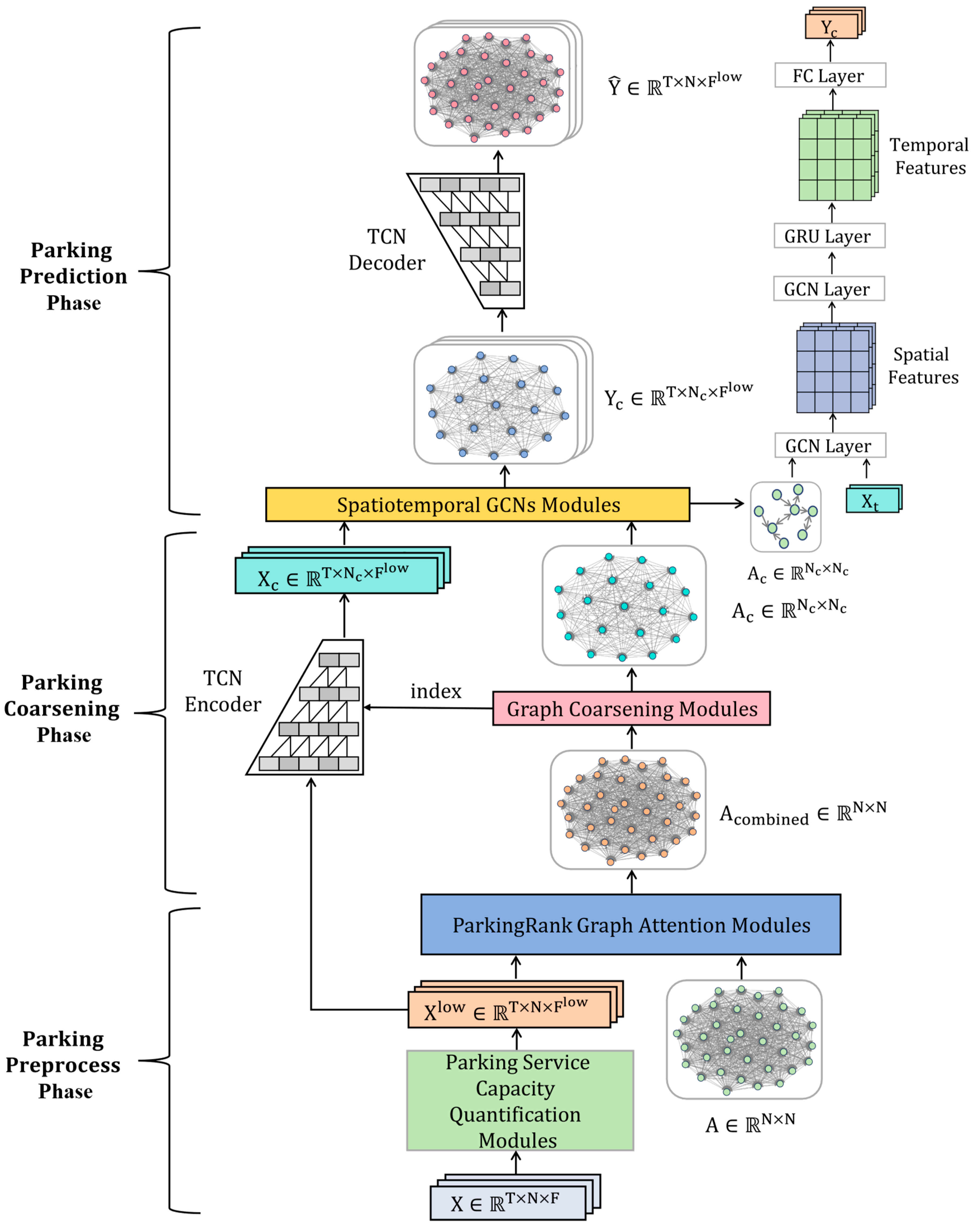
• We introduce a novel framework for parking prediction that employs a graph coarsening techniques and temporal convolutional autoencoder [30], designed to diminish the resource and time expenditures associated with urban parking prediction models. The scheme can make up for the shortcomings of traditional coarsening methods that neglect the dimensionality reduction of node features, and realize the unified dimensionality reduction of urban parking graph structure and features. Moreover, by incorporating temporal convolutional networks in the encoding-decoding phase, our approach not only significantly enhances the dimensionality reduction and reconstruction capabilities for parking time series data but also ensures the accuracy of the parking prediction task. Additionally, the compact data volume within each hypernode allows for the parallel processing of encoding-decoding operations across different sets of parking time series data, further boosting the overall training efficiency of the parking prediction task.

This paper is structured as follows: Section 2 provides a concise overview of spatio-temporal GCNs for parking prediction, techniques for dimensionality reduction in large-scale graphs, and the applications of Autoencoders (AE). Section 3 delves into the specifics of our innovative ParkingRank graph attention model and outlines our parking prediction methodology, which leverages TCN-AE for coarsening. Section 4 details the experimental framework and analysis employed to assess the effectiveness of our proposed approach. We conclude by summarizing the key insights and contributions of this study.

2. Related WORK

2.1. Spatio-Temporal Graph Convolutional Models

Spatio-temporal GCNs [31] have emerged as a powerful and prevalent approach within the realm of traffic prediction, adept at navigating the intricacies of traffic graphs by integrating both spatial and temporal dependencies. Unlike relying solely on GCNs or RNNs, spatio-temporal GCNs excel at dissecting time-series data embedded in graph structures [32], thereby yielding more precise prediction. For instance, Zhao et al. [33] introduced the T-GCN model, ingeniously combining GCN with GRU to understand the intricate topology of traffic networks and the dynamic shifts in traffic data, enhancing the capture of spatio-temporal characteristics more effectively. In a similar vein, Sun et al. [34] unveiled DDSTGCN, leveraging TCN to track variations in traffic states alongside GCN for topology learning, markedly boosting traffic prediction accuracy. In recent years, scholars have suggested employing attention mechanisms to bolster the extraction of spatio-temporal features, thereby extending the model’s interpretability. Zheng et al. [35] proposed a novel strategy that incorporates spatial and temporal attention layers to elucidate the spatio-temporal correlations within heterogeneous traffic flows, thereby not only elevating predictive performance but also the interpretability of the findings. Furthermore, Li et al. [36] developed AST-GAT, incorporating multi-head graph attention and attention-based LSTM modules to intricately map the spatio-temporal interdependencies among road segments, aiming to refine the precision of traffic prediction.

Due to the inherent structural and functional similarities between urban transportation networks and urban parking networks, both involve complex spatial relationships and dynamically changing temporal characteristics. Leveraging advanced spatio-temporal graph convolutional models from the field of traffic prediction, we believe can effectively enhance the accuracy of parking prediction. However, in the domain of parking prediction, the industrial sector continues to prioritize concerns regarding time costs and resource consumption, with a current lack of effective solutions. These challenges will limit the feasibility and effectiveness of the aforementioned spatio-temporal graph convolutional models in practical industrial applications.

2.2. Techniques for Dimensionality Reduction in Large-Scale Graphs

As the scale of graphs continues to expand, finding a universal method that can simplify the structure while preserving key attributes becomes increasingly important. Simplified graph representations not only facilitate storage but also offer efficiency in approximate algorithms [20]. There are mainly two methods for simplifying graphs: The first method, known as graph sparsification [37], approximates the maintenance of distance relationships between node pairs by removing edges from the graph. However, for highly structured parking graphs, this method might lose the original graph’s connectivity. An improved method is the K-neighbors Sparsifier [38], which performs local sparsification on each node by setting a threshold, but still introduces high computational complexity. With the growing popularity of deep learning, Wu et al. [39] proposed GSGAN, which generates new graphs through GANs to preserve the community structure of the original graph, but it introduces edges that do not exist in the original graph and contradicts reality.

The second approach is known as graph coarsening [40], which aims to reduce the number of nodes to a subset of the original nodes while maintaining the original graph properties. The key to graph coarsening [21] lies in the ability to accurately measure the variations before and after coarsening. The GraClus [41] technique, and the MCCA [42] algorithm all employ the idea of greediness by constantly compacting the connected regions of the original graph. However, these approaches lack guarantees for global optimization. Recently, spectral graph theory [22] proved that graphs with similar spectra are usually considered to have similar topologies. Therefore, the idea of minimizing the spectral distance can be introduced into the coarsening process, using the eigenvalues of the graphs to measure the structural similarity and ensuring that the generated coarsened graphs can maintain the properties of the original graphs.

However, we have observed that current graph coarsening methods primarily focus on reducing the complexity of the graph structure while often neglecting the dimensionality of node features. This approach does not effectively reduce the actual volume of parking data in large-scale urban parking prediction tasks. Although the parking network structure has been somewhat simplified through graph coarsening techniques, the training overhead for downstream parking prediction models has not decreased as significantly as anticipated.

2.3. Applications of Autoencoders

AEs have demonstrated remarkable proficiency in managing intricate spatio-temporal data relevant to transportation systems [35]. Typically employing symmetrically structured encoders and decoders for unsupervised learning, these AEs are adept not only at distilling input data into compact representations of potential vectors [27], but also at restoring the data to its original dimensions. They achieve this by optimizing the reconstruction of the data’s objective, thereby minimizing loss [29]. For instance, the TGAE introduced by Wang et al. [43] adeptly captures the underlying patterns of traffic flow through a spatio-temporal AE, facilitating the prediction of future traffic information. Similarly, the TCN-AE devised by Mo et al. [44] leverages TCNs within its encoding module to extract features from temporal data, subsequently utilizing the decoding module to map latent representations back to the original data space, thus enabling anomaly detection.

Inspired by the capabilities of AEs in dimensionality reduction and key feature extraction of spatio-temporal data, we propose the integration of AEs into large-scale urban parking prediction tasks, aiming to address the limitations of traditional coarsening methods in handling parking lot node features. Additionally, by leveraging the advantages of TCN in processing complex temporal data, AEs can more accurately capture and analyze the parking patterns within different parking lots, thereby significantly enhancing the performance and depth of understanding of downstream parking prediction models.

3. Methodology

3.1. Problem Definition

In this paper, our goal is to effectively reduce the time and resource costs of parking prediction models by achieving a unified reduction in the dimensions of the structure and feature data of urban parking graphs, while ensuring the accuracy of parking prediction tasks. The urban parking graph can be represented as $G=(V,E,A)$, where V denotes the set of parking nodes, E denotes the set of edges, and $A\in {\mathbb{R}}^{N\times N}$ denotes the directed adjacency matrix, $N=\left|V\right|$.

The parking prediction problem [12] can be interpreted as: given a parking graph G and historical parking data $X_{(t-T+1):t}$ for T time slices before time t, learning a function F to predict future parking data ${\widehat{Y}}_{(t+1):(t+T^{\prime })}$ for $T^{\prime }$ time slices after time t, as shown in Equation 1.

$${\widehat{Y}}_{(t+1):(t+T^{\prime })}=F(X_{(t-T+1):t},G),$$

(1)

where the parking data $X=\{x_1,x_2,\dots ,x_T\}\in {\mathbb{R}}^{T\times N\times F}$ represents the parking flow information observed at T time slices for all parking lots. Each $x_t$ corresponds to a time slice and includes N parking lot nodes, each with F dimensional features, including the longitude, latitude, openness to the public, charging situation, and real-time occupancy rate of the parking lot.

3.2. ParkingRank Graph Attention

Graph coarsening, as the current mainstream graph dimensionality reduction technique, aims to overcome the huge computational obstacles faced by large-scale graph data when processing, extracting and analyzing. Typically, the input for graph coarsening is the graph adjacency matrix [21]. When dealing with complex structures such as urban parking graphs, the traditional adjacency matrix constructed from topological relationships is obviously difficult to adequately capture the complexity and diversity of the real parking landscape. In fact, drivers do not only consider the proximity of parking lots in the region when making parking decisions, but also comprehensively compare the distance of regional parking lots, real-time space occupancy rate, openness to the public, and charging situation, and other factors. Therefore, before performing the task of urban parking graph coarsening, we need a high-quality parking graph that can truly reflect the preference of parking behavior and adapt to the dynamic change of parking demand.

GAT [45] is an advanced spatial-based graph neural network methodology, whose primary advantage lies in redefining the aggregation of node features. Unlike GCN that typically assign equal weights to all neighboring nodes for information aggregation, GAT introduces an attention mechanism. This allows the model to dynamically allocate varying weights based on the importance of each neighboring node. Such a strategy enables GAT to more effectively capture spatial correlations within road networks and selectively emphasize those nodes that are crucial for the current task. In the application of urban parking network prediction, this feature of GAT is particularly significant. It enables the network to flexibly capture important relationships between parking nodes, focusing on those nodes that are critical for the current prediction task. We believe that this not only helps in more accurately describing the correlations between different parking lots but also aids in constructing an efficient parking network that reflects the relevancy of parking spaces. The overall framework of our proposed PRGAT is shown in Figure 1:

Given the complexity of the parking data X directly inputting the high-dimensional data $x_t$ into GAT would lead to considerable computational redundancy, thereby increasing the model’s time cost. To address this, we adopt a dimensionality reduction strategy that involves extracting and abstracting certain features of the parking lots. This effectively reduces the computational burden and enhances the model’s computational efficiency.

The ParkingRank model [25] is an algorithm to quantitatively assess the service capability of different parking lots. By integrating complex parking information such as the total number of parking spaces in the parking lot, the degree of openness to the public, and the price of parking, it can help drivers to understand the actual situation of the parking lot in a more comprehensive way, so that they can make informed choices in the parking decision-making process. Specifically, the algorithm primarily focuses on three aspects to describe the real-time service capacity of parking lots, as shown in Equation 2:

• Parking lot service range: This aspect considers which types of vehicles are allowed to park in the parking lot. For example, parking lots at shopping centers may be open to all vehicles, while those in residential areas may only serve residents. Therefore, parking lots with a broader service scope generally have stronger service capabilities.
• Total number of parking spaces: The more internal parking spaces a parking lot has, the stronger its service capacity usually is.
• Price of parking: Higher parking prices may reduce the number of vehicles able to afford parking fees. Thus, expensive prices may lower the service capacity of the parking lot.

$$P{R}_i=exp\left(s_i\right)\frac{\left(y_i/\parallel y\parallel \right)}{1+z_i/\parallel z\parallel },$$

(2)

where $P{R}_i$ represents the service capacity of each parking lot; $s_i\in [0,1]$ denotes the service range, which is used to measure the degree of openness of the parking lot, from the public parking lot ($s_i=1$) to the private parking lot ($s_i=0$); $y_i$ and $z_i$ represent the total number of parking spaces and the price of parking, respectively. $\parallel y\parallel$ and $\parallel z\parallel$ are the first-order paradigms for the y- and z-column vectors.

We believe that the process of quantifying the service capability of a parking lot is essentially a process of extracting the redundant parts of the parking lot features $x_t$, and the low-dimensional evaluation results can be used as new abstract features to replace the original high-dimensional parking data $x_t$.

Moreover, while GAT typically utilize Multi-Layer Perceptrons (MLP) or cosine similarity to ascertain the degree of association between nodes, such conventional methods may fall short in terms of interpretability, particularly when applied to entities like parking lots with distinct attributes. These methods often fail to offer a clear insight into the dynamics of parking lot interactions. To mitigate the black-box issue encountered by GATs in analyzing parking graphs, we integrate the parking spatio-temporal transfer matrix [2] into the computation of attention coefficients within GATs. This matrix meticulously accounts for the spatio-temporal evolution of parking lot features, encompassing real-time occupancy rates, service capabilities, and spatial connections, thereby facilitating a dynamic representation of parking cruising behavior. This nuanced incorporation allows for a richer, more detailed understanding of parking dynamics, effectively translating the raw data into actionable insights. The formulation of this transfer matrix $A_{trf}$ is presented in Equation 3.

$$A_{\mathrm{trf}}=\left\{\begin{array}{c}{q}_i,\mathrm{when}i=j\\ w_{i,j}\left(1-{\mathrm{q}}_j\right)P{R}_i,\mathrm{when}i\ne j\end{array}\right.,$$

(3)

where each element ${\alpha }_{i,j}^{\mathrm{trf}}$ of $A_{\mathrm{trf}}\in {\mathbb{R}}^{N\times N}$ represents the probability of a vehicle heading to another parking lot j when it finds parking lot i is full. $q_i$ represents the real-time occupancy rate of parking lot i, which also indicates the probability of a vehicle choosing to stay in parking lot i based on the parking situation. $w_{i,j}$ is the reciprocal of the normalized distance $A_{i,j}$ between parking lot i and parking lot j. $P{R}_i$ is the normalized service capacity of parking lot i.

Therefore, in this paper, the input to PRGAT consists of the original adjacency matrix A based on Euclidean distance and the new parking data $X^{\mathrm{low}}\in {\mathbb{R}}^{T\times N\times F^{\mathrm{low}}}$, which is composed of the service capacity $P{R}_i$, the real-time occupancy rate $q_i$, and latitude and longitude coordinates. The output is the updated parking data $X^{\mathrm{re}}\in {\mathbb{R}}^{T\times N\times F^{\mathrm{re}}}$. Here, $F^{\mathrm{low}}$ represents the new feature dimensions after quantification and extraction, while $F^{\mathrm{re}}$ denotes the new feature dimensions relearned by PRGAT.

The algorithm initially applies a linear transformation to each parking lot node’s features $x_t^{\mathrm{low}}\left(i\right)$ using a learnable weight matrix $W\in {\mathbb{R}}^{F^{\mathrm{re}}\times F^{\mathrm{low}}}$ to enhance the node’s expressive capability. Subsequently, it employs an attention mechanism $\mathcal{T}$ on the set of nodes to compute the attention coefficient $e_{i,j}$ between node i and node j. This procedure can be encapsulated by Formula 4, wherein the attention mechanism might be a function that signifies the correlation between two objects, like cosine similarity or a Multilayer Perceptron (MLP), and ∥ represents the vector concatenation operation.

$$e_{i,j}=\mathcal{T}\left[W{x}_t^{\mathrm{low}}\left(i\right)\parallel W{x}_t^{\mathrm{low}}\left(j\right)\right],$$

(4)

To capture local topological information and enhance computational efficiency, a masking mechanism and normalization operation have been introduced. The attention coefficients $e_{i,j}$ are confined within the first-order neighborhood of the nodes, enabling each node to concentrate solely on its directly connected neighboring nodes and disregard the other nodes in the graph, ultimately yielding the attention matrix $A_{\mathrm{attn}}\in {\mathbb{R}}^{N\times N}$. See Formula 5 for details, where LeakyReLU represents the activation function.

$$A_{\mathrm{attn}}(i,j)={\alpha }_{i,j}^{\mathrm{attn}}={\displaystyle \frac{exp\left(LeakyReLU\left(e_{i,j}\right)\right)}{{\sum }_{k\in N_i}exp\left(LeakyReLU\left(e_{i,k}\right)\right)}},$$

(5)

Moreover, the masking mechanism ingeniously reflects the factors influencing the parking decision-making process. Drivers, when choosing a parking lot, tend to compare a specific parking lot with its adjacent ones, rather than conducting pairwise comparisons among all parking lots. Such a masking mechanism not only enhances the model’s sensitivity to local associations but also aligns more closely with the behavioral patterns in the actual parking decision-making process.

We input both the parking spatio-temporal transfer matrix $A_{\mathrm{trf}}$ and the aforementioned attention matrix $A_{\mathrm{attn}}$ into the softmax activation function simultaneously to derive the ParkingRank attention matrix $A_{\mathrm{combined}}\in {\mathbb{R}}^{N\times N}$, as indicated in Equation 6.

$$A_{\mathrm{combined}}(i,j)={\alpha }_{i,j}^{\mathrm{combined}}=softmax\left({\alpha }_{i,j}^{\mathrm{trf}}+{\alpha }_{i,j}^{\mathrm{attn}}\right),$$

(6)

This ParkingRank attention matrix not only reflects the dynamic characteristics of the parking graph, capturing the flow trajectories and behavioral patterns of vehicles in urban parking scenarios, but also overcomes the shortcomings of insufficient interpretability of the parking lot relevance matrix computed by traditional graph attention methods.

After obtaining the normalized ParkingRank attention coefficients ${\alpha }_{i,j}^{\mathrm{combined}}$, GAT conducts a weighted aggregation of the features of each node i with its neighbors $N_i$, thereby producing the final output for each node. This procedure is depicted in Formula 7, where $\sigma$ denotes the sigmoid activation function.

$$x_t^{re}\left(i\right)=\sigma \left(\sum _{j\in N_i}{\alpha }_{i,j}^{\mathrm{combined}}W{x}_t^{\mathrm{low}}\left(j\right)\right),$$

(7)

The PRGAT we designed is fundamentally a pre-trained model, its primary purpose being to serve as a front-end graph construction module within the overall framework for urban parking prediction. Its loss function is described in Formula 8, and the pseudocode for the graph is provided in Algorithm 1.

$$L_{GAT}\left(X^{\mathrm{low}},X^{\mathrm{re}}\right)={\displaystyle \frac{1}{T}}\sum _{i=t-T+1}^t{∥X^{\mathrm{low}}\left(i\right)-X^{\mathrm{re}}\left(i\right)∥}^2,$$

(8)

Algorithm 1: ParkingRank Graph Attention (PRGAT)

Input: $A\in {\mathbb{R}}^{N\times N},X\in {\mathbb{R}}^{T\times N\times F}$ Output: $A_{\mathrm{combined}}\in {\mathbb{R}}^{N\times N},X^{\mathrm{re}}\in {\mathbb{R}}^{T\times N\times F_{\mathrm{re}}}$ 1: $W\leftarrow \mathrm{MLP}(X,F^{\prime })$  2: $a\leftarrow \mathrm{Correlation}(2\times F,F^{\prime })$  3: $A_{\mathrm{attn}}\leftarrow \mathrm{Zeros}(N,N)$  4: $A_{\mathrm{trf}}\leftarrow \mathrm{Zeros}(N,N)$  5: for$i\leftarrow 1\mathrm{to}N$do  6:    $P{R}_i\leftarrow \mathrm{ParkingServiceCapacity}\left(X\left(i\right)\right)$  7:    $X^{\mathrm{low}}\left(i\right)\leftarrow \mathrm{ParkingReconstruction}(P{R}_i,X\left(i\right))$  8: end for 9: for$i\leftarrow 1\mathrm{to}N$do  10:    $q_i\leftarrow \mathrm{ParkingOccupancyRate}\left(X^{\mathrm{low}}\left(i\right)\right)$  11:    for $j\leftarrow 1\mathrm{to}N$ do  12:      $s_{i,j}\leftarrow \mathrm{Normalized}\left(A(i,j)\right)$  13:      ${\alpha }_{i,j}^{\mathrm{trf}}\leftarrow s_{i,j}*(1-q_i)*P{R}_i$  14:      $e_{i,j}\leftarrow \mathrm{Concat}(W{X}^{\mathrm{low}}\left(i\right),W{X}^{\mathrm{low}}\left(j\right))$  15:      ${\alpha }_{i,j}^{\mathrm{ReLU}}\leftarrow \mathrm{LeakyReLU}(a^T*e_{i,j})$  16:      ${\alpha }_{i,j}^{\mathrm{Masked}}\leftarrow \mathrm{MaskedFill}({\alpha }_{i,j}^{\mathrm{ReLU}},A(i,j))$  17:      ${\alpha }_{i,j}^{\mathrm{attn}}\leftarrow \mathrm{Normalized}\left({\alpha }_{i,j}^{\mathrm{Masked}}\right)$  18:      $A_{\mathrm{combined}}(i,j)\leftarrow \mathrm{softmax}({\alpha }_{i,j}^{\mathrm{attn}}+{\alpha }_{i,j}^{\mathrm{trf}})$  19:    end for  20: end for  21: $X^{\mathrm{re}}\leftarrow \sigma \left(A_{\mathrm{combined}}W{X}^{\mathrm{low}}\right)$  22: return$A_{\mathrm{combined}},X^{\mathrm{re}}$

3.3. Parking Graph Coarsening

Define the coarsened parking graph $G_c=(V_c,E_c,A_c)$ is the result of coarsening the original adjacency matrix A, which is a smaller weighted graph. $V_c$ denotes a set of disjoint hypernodes, which covers all nodes in the original graph V, where each hypernode is formed by the aggregation of some of the nodes in the original graph, i.e., $v_i^c=\{v_1,v_2,\dots ,v_n\}\in {\mathbb{R}}^N$. $A_c\in {\mathbb{R}}^{N_c\times N_c}$ is the adjacency matrix of the coarsened graph, $N_c=\left|V_c\right|$.

This document employs the SGC algorithm [22], which utilizes spectral distance (SD) to demonstrate that the coarsened network retains spatial features similar to those of the original network. This concept is illustrated in the equation below:

$$SD\left(G,G_c\right)={∥\lambda -{\lambda }_c∥}_1=\sum _{i=1}^N\left|\lambda \left(i\right)-{\lambda }_c\left(i\right)\right|,$$

(9)

where the vectors $\lambda$ and ${\lambda }_c$ represent the eigenvalues of the Laplacian matrices of the original graph G and the coarsened graph $G_c$, respectively. The spectral distance $SD(G,G_c)$ is considered sufficiently small if it is less than $\delta$ (where $\delta$ is a very small number). Only when this condition is met do the eigenvalues and eigenvectors of the two graphs exhibit similarity in the spectral domain. The calculated spectral distance can then substantiate that the coarsened graph significantly preserves the attributes of the original graph during the coarsening process. Thus, it can be inferred that the spatial structure of the coarsened network remains similar to that of the original network. The key steps of the SGC algorithm are introduced below.

The algorithm initiates by inputting the ParkingRank attention matrix $A_{\mathrm{combined}}$ and the coarsening ratio $n={\displaystyle \frac{N_c}{N}}$. It computes the Laplacian matrix $\mathcal{L}$ and, through matrix decomposition, obtains the first $N_c$ and the last $N-N_c+1$ Laplacian eigenvalues $\lambda$ and Laplacian eigenvectors u, for capturing both the local and global information of the parking graph. This procedure is illustrated in Formulas 10 and 11, wherein $\mathcal{L}$ signifies the normalized Laplacian matrix, with $I_N$ and D being the identity matrix and the degree matrix, respectively.

$$\mathcal{L}=I_N-D^{-1/2}{A}_{\mathrm{combined}}{D}^{-1/2},$$

(10)

$$\mathcal{L}u=\lambda Du,$$

(11)

Then, the algorithm starts to iterate different eigenvalues intervals, performs parking clustering on the internal eigenvectors u respectively, divides the parking lots with similar features into a parking hypernode, and generates a preliminary coarsened graph $G_c$ based on the clustering results, the clustering principle is shown in Equation 12.

$$d_c(i,j)={\displaystyle \frac{{\sum }_{i=1,j=1}^n{u}_i{u}_j}{\sqrt{{\sum }_{i=1}^n{\left(u_i\right)}^2}\sqrt{{\sum }_{j=1}^n{\left(u_j\right)}^2}}},$$

(12)

The Laplacian eigenvectors u computed from the ParkingRank attention matrix $A_{combined}$ has rich parking graph topology information as well as parking lot node feature information, which can provide more accurate and intuitive parking lot node characterization for the coarsening process.

The process continuously calculates the distance $SD$ between the Laplacian eigenvectors of the coarsened graph $G_c$ and those of the original graph, opting for the coarsening outcome with the minimum error. Finally, the coarsened graph $G_c=(V_c,E_c,A_c)$ along with the corresponding index matrix $index$ are returned. This procedure is depicted in Formula 13, with the coarsening specifics provided in Algorithm 2.

$$SD\left(A_{\mathrm{combined}},A_c\right)={∥d_{\mathrm{combined}}\left(i\right)-d_c\left(i\right)∥}_1,$$

(13)

Algorithm 2: Parking graph Coarsening

Input: $A_{\mathrm{combined}}\in {\mathbb{R}}^{N\times N},n$ Output: $A_c\in {\mathbb{R}}^{N_c\times N_c},\mathrm{index}\leftarrow \left[\right]$  1: $N_c\leftarrow \mathrm{CoarsenedNodesNum}(n,N)$  2: $\mathcal{L}\leftarrow \mathrm{NormalizedLaplacian}\left(A_{\mathrm{combined}}\right)$  3: $\lambda ,u\leftarrow \mathrm{EigenValueAndVector}(L,N_c)$  4: for$i\leftarrow 1\mathrm{to}N$do  5:    for $j\leftarrow 1\mathrm{to}\mathrm{Neighbor}\left(i\right)$ do  6:      $A_c^{\mathrm{temp}},\mathrm{index}\leftarrow \mathrm{ParkingSubZoneClustering}(u_i,u_j)$  7:    end for  8: end for  9: for$i\leftarrow 1\mathrm{to}N$do  10:    for $j\leftarrow 1\mathrm{to}N$ do  11:      $A_c\leftarrow argmin\mathrm{SD}(A_{\mathrm{combined}}(i,j),A_c(i,j))$  12:    end for  13: end for  14: return$A_c,\mathrm{index}$

3.4. Prediction Framework Based on Coarsened Parking Graphs

Since the coarsening process of the parking graph described above does not downscale the parking lot node features, the feature data corresponding to the parking hypernodes $X^{\mathrm{combined}}\in {\mathbb{R}}^{T\times N\times F^{\mathrm{low}}}$ remains a splicing operation between the merged parking lot data, which is formalized as follows:

$$x_t^{\mathrm{combined}}\left(i\right)=\sum _{j\in v_i^c}{x}_t^{\mathrm{low}}\left(i\right)\parallel x_t^{\mathrm{low}}\left(j\right),$$

(14)

If it is simply used as the feature input for the parking prediction models, it will not significantly improve the overall framework training efficiency, and even lose the intrinsic connection between the nodes. In this regard, we consider adopting the symmetric TCN-AE, which is because:

• TCN is able to mine the intrinsic laws behind the parking time-series data itself [44], such as the tidal characteristics, which helps in the compression and reconstruction of the parking data.
• The encoder is able to embed the high-dimensional sparse parking data into the low-dimensional dense tensor form, which reduces the computational overhead of the training model.
• The decoder is able to achieve an approximate lossless reduction and can reconstruct the spatial structure of the original parking graph.

To maintain the consistency of the prediction results between the coarsened and the original parking graphs, we train a set of symmetric TCN-based AEs for each parking hypernode, utilizing the index matrix generated by the graph coarsening module. TCNs typically consist of multiple layers of dilated causal convolution, with each layer performing one-dimensional convolution. Moreover, to enhance the network’s expressive capacity, residual connections are often added following multiple convolutional layers, organizing these layers into several residual blocks. Each residual block primarily includes two dilated causal convolution layers, interspersed with normalization, activation, and dropout operations, before the output is added to the input of the next residual block. This design not only optimizes the flow of information but also enhances the model’s ability to capture features of parking data effectively.

The procedure is detailed as follows: As depicted in Figure 2, firstly, the parking data $X^{\mathrm{low}}\in {\mathbb{R}}^{T\times N\times F^{\mathrm{low}}}$ undergoes encoding with the residual blocks within the encoder [44], as indicated in Formula 15. Owing to the reduction in the number of features as the quantity of residual blocks increases, it allows the feature data $X_c\in {\mathbb{R}}^{T\times N_c\times F^{\mathrm{low}}}$ corresponding to the coarsened graph to be represented within a low-dimensional feature space.

$$X_c\left(i\right)=\left(X^{\mathrm{low}}*f\right)\left(i\right)=\sum _{j=0}^{k-1}f\left(j\right)X^{\mathrm{low}}(i-j),$$

(15)

where ${\sum }_{j=0}^{k-1}f\left(j\right)$ denotes the filter f of length k and * denotes the convolution operation. This formula ensures that only information prior to the current time step is considered and future information is not computed.

Next, we input the adjacency matrix $A_c$ of coarsened graph and feature matrix $X_c$ into a spatio-temporal graph convolutional model. This paper takes T-GCN [33] as an example, which captures the spatio-temporal dependencies of the parking coarsened graph through 2 layers of GCN and 1 layer of GRU, finally obtaining the coarsened graph’s predicted results $Y_c\in {\mathbb{R}}^{T\times N_c\times F^{\mathrm{low}}}$ through a linear transformation, as seen in Formulas 16, 17, 18, 19, and 20, where W and b represent the weights and biases of T-GCN, respectively, and $u_t$, $r_t$, $c_t$, $h_t$ denote the reset gate, update gate, candidate hidden state, and current hidden state at time t,respectively. $gc\left(·\right)$ denotes the graph convolution operation, and tanh is the activation function.

$$u_t=\sigma \left(W_u·\left[gc\left(X_c,A_c\right),h_{t-1}\right]+b_u\right),$$

(16)

$$r_t=\sigma \left(W_r·\left[gc\left(X_c,A_c\right),h_{t-1}\right]+b_r\right),$$

(17)

$$c_t=tanh\left(W_c·\left[gc\left(X_c,A_c\right),\left(r_t,h_{t-1}\right)\right]+b_c\right),$$

(18)

$$h_t=u_t*h_{t-1}+\left(1-u_t\right)*c_t,$$

(19)

$$Y_c=softmax\left(W_y·h_t+b_y\right),$$

(20)

Due to the fact that the dimensions of the coarsened graph’s predicted results $Y_c$ do not align with the size of the original parking graph, these results are not inherently interpretable. To address this, decoding is necessary. Based on the prediction length, we opt for a particular pre-trained decoder, inputting the prediction of each hypernode to reconstruct the original parking graph’s prediction results $\widehat{Y}\in {\mathbb{R}}^{T\times N\times F^{\mathrm{low}}}$, thereby fulfilling the prediction task for the entire urban parking graph. The decoding procedure is depicted in Formula 21. $f^{-1}$ denotes the filters within the decoder, distinct from the encoding phase, as the feature count in the decoder’s residual blocks grows with the increase in residual blocks, aiming to reconstruct parking data within a high-dimensional feature space.

$$\widehat{Y}\left(i\right)=\left(Y_c*f^{-1}\right)\left(i\right)=\sum _{s=0}^{T-1}\sum _{i=0}^{k-1}{f}^{-1}\left(i\right)Y_c\left(i\right),$$

(21)

The loss functions for the pre-trained TCN-AE and the parking prediction model utilize Mean Squared Error (MSE) and Huber Loss, respectively, as detailed in Formulas 22 and 23. In this context, $\widehat{X}\in {\mathbb{R}}^{T\times N\times F^{\mathrm{low}}}$ represents the outcome post-reconstruction by the autoencoder, Y signifies the real observed data, and $\theta$ represents the threshold parameter that controls MSE.

$$L_{AE}\left(X^{\mathrm{low}},\widehat{X}\right)={\displaystyle \frac{1}{T^{\prime }}}\sum _{i=t-T^{\prime }+1}^t{∥X^{\mathrm{low}}\left(i\right)-\widehat{X}\left(i\right)∥}^2,$$

(22)

$$L_{\mathrm{predict}}(Y,\widehat{Y})=\left\{\begin{array}{c}{\displaystyle \frac{1}{2}}{(Y-\widehat{Y})}^2,|Y-\widehat{Y}|\le \theta \\ \theta |Y-\widehat{Y}|-{\displaystyle \frac{1}{2}}{\theta }^2,\mathrm{otherwise}\end{array}\right.,$$

(23)

4. Experiments

4.1. Experiment Setup

This paper selected 9000 parking lots within five districts including Bao’an and Luohu in Shenzhen as research subjects. The parking data recorded for six months starting from June 1, 2016, was sampled at 15-minute intervals. These datasets encompassed key information such as the geographic coordinates, open status, pricing details, and real-time occupancy of each parking lot. To ensure data quality, we conducted deduplication and visualization-based outlier detection operations on the raw parking data. Additionally, to maintain consistency in data processing, all datasets underwent normalization before analysis. Finally, we partitioned the dataset chronologically into training set (70%), validation set (20%), and test set (10%) to ensure the validity and reliability of the experiments. Specifically, the distribution of parking lots in Bao’an District was visually presented through Figure 3, and specific details of the parking lot data are referred to in Table 1.

To evaluate the performance of our method, we selected several commonly used evaluation metrics in regression tasks: MAE, RMSE, and MAPE. The expressions for these metrics are as follows:

$$\begin{array}{cc}\hfill \mathrm{MAE}& ={\displaystyle \frac{1}{TN}}\sum _{t=1}^T\sum _{i=1}^N|y_t^i-{\widehat{y}}_t^i|\hfill \\ \hfill \mathrm{RMSE}& =\sqrt{{\displaystyle \frac{1}{TN}}{\sum }_{t=1}^T{\sum }_{i=1}^N{(y_t^i-{\widehat{y}}_t^i)}^2}\hfill \\ \hfill \mathrm{MAPE}& ={\displaystyle \frac{100\%}{TN}}\sum _{t=1}^T\sum _{i=1}^N\left|{\displaystyle \frac{y_t^i-{\widehat{y}}_t^i}{y_t^i}}\right|\hfill \end{array}$$

(24)

where ${\widehat{y}}_t^i$ and $y_t^i$ respectively represent the predicted result and the ground truth for the i-th parking lot at time t. T denotes the length of the time sample, and N is the total number of parking lot nodes.

In the experimental parameter design, we use data from the past 12 time steps to predict data for the next 1, 2, and 4 steps, which corresponds to using the past 3 hours of parking traffic to predict the parking traffic for the next 15 minutes, 30 minutes, and 60 minutes, respectively. Additionally, to evaluate the predictive performance, we selected three widely used baseline models in the parking prediction field for comparison. Additionally, to explore the effectiveness of graph coarsening techniques, we also employed the recently popular graph sparsification methods as a benchmark:

• T-GCN [33]: A classical model for traffic prediction that combines Graph Convolutional Networks (GCNs) and Gated Recurrent Units (GRU) to establish spatio-temporal correlations among traffic data.
• STGCN [46]: Utilizes multiple ST-Conv blocks to model multi-scale traffic graphs, proven to effectively capture comprehensive spatio-temporal correlations.
• STSGCN [47]: By stacking multiple STSGCL blocks for synchronous spatio-temporal modeling, it can effectively capture complex local spatio-temporal traffic correlations.
• SparRL [37]: A universal and effective graph sparsification framework implemented through deep reinforcement learning, capable of flexibly adapting to various sparsification objectives.

For the training of various models, we utilized V100 graphics cards and implemented early stopping and dynamic learning rate adjustment mechanisms to optimize the training process. To ensure completeness and transparency of information, we have listed the configuration details of the models along with all training-related hyperparameters in Table 2.

4.2. Modeling Real Scenes

To demonstrate the graph construction process of the PRGAT method, we conducted an experiment using real parking lot data from Bao’an District in Shenzhen. In Bao’an District, the number of parking lots exceeds 1,000, leading to the number of reachable edges between parking lots reaching the order of millions. Therefore, to simplify the analysis while ensuring the practicality of the results, we selected a more central CBD area within the district as the study area, which contains over 600 parking lots. Additionally, we set a spatial distance threshold of 500 meters; distances between any parking lots exceeding this threshold were considered unreachable to align with real parking scenarios.

Shown in Figure 4 is a visualization of the parking graph constructed using the PRGAT model for the Baoan core area around evening during the week, where the different sizes of circles represent the service capacity of the parking lots, with larger circles implying stronger service capacity and more popularity among drivers. Unlike the traditional spatial adjacency matrix, the dynamic adjacency matrix generated by PRGAT can intuitively reflect the real-time importance of each parking lot, which helps the downstream prediction model to accurately determine the key parking lots in each time period, thus effectively identifying the places with strong or weak parking demand. Meanwhile, the graph composed of these parking lots with strong service capacity essentially depicts the parking backbone network of the city in different time periods, and this dynamic parking backbone network reflects the core areas and hotspots of the city’s parking demand, which provides an important perspective for understanding the city’s parking behavior pattern.

Figure 5 depicts the distribution of parking lots in the core area of Bao’an under different coarsening ratio (coarsened vertices/original graph vertices). By adjusting the coarsening ratio, we can clearly see significant changes in the structure and density of the parking graph: parking lots with stronger service capacities gradually absorb those with weaker capacities, thus forming larger parking hypernodes with enhanced comprehensive service capabilities. As the ratio of coarsening is progressively reduced, the backbone of the urban parking graph also becomes clearer. However, this coarsening process also poses certain challenges: a simplified parking graph means the loss of some important parking information, which could affect the downstream model’s ability to capture details, especially in areas highly sensitive to parking demand or where demand changes rapidly.

4.3. Selection of Coarsening Ratio

Considering the dual role of the coarsening ratio in the speed of model convergence and model prediction accuracy, we set up control experiments with coarsening ratio of 0.2, 0.3, 0.4, 0.5, 0.6, 0.7, 0.8, 0.9, and without coarsening (coarsening ratio of 1), to study the impact of different coarsening ratio on the prediction of parking occupation rate during the evening rush hour. The prediction results are shown in the Figure 8, where dashed and solid lines respectively represent the impact of different coarsening ratio on model prediction accuracy and convergence speed.

As seen in Figure 6, as the coarsening ratio decreases from 1 to 0.6, the error growth rate of the model predictions remains relatively stable. This indicates that within this range of coarsening ratio, the model primarily loses redundant and secondary parking information, the absence of which has limited impact on overall prediction accuracy. However, as the coarsening ratio is further reduced, the prediction error of the models rapidly increases, particularly when the coarsening ratio is adjusted to 0.2, introducing calculation errors of 77.2%, 64.2%, and 61.8%, respectively. This suggests that crucial parking information (such as the highly volatile characteristics of parking lots) has been stripped away in the coarsening process.

Figure 6. Impact of Different Coarsening Ratio on Prediction Performance.

Figure 6. Impact of Different Coarsening Ratio on Prediction Performance.

It’s noteworthy that the curve of model training duration presents a different trend. With the reduction of the coarsening ratio, the initial training time decreases rapidly, showing that coarsening can significantly reduce the computational burden of the model. However, after reaching a coarsening ratio of 0.6, the trend of reduction in training duration becomes more gradual, indicating that further coarsening does not significantly enhance efficiency. Specifically, in the coarsened graph, nodes of parking lots with significantly different characteristics may be merged, leading to a loss of crucial detail information that was originally observable. Consequently, the model’s ability to distinguish these differences is impaired, thereby affecting its predictive and generalization capabilities.

The two sets of experiments indicate that the ideal coarsening ratio should be within the range of 0.5 to 0.6. Coarsening within this interval manages to strike a balance between simplifying model complexity and retaining key feature information, which is particularly crucial when dealing with large-scale urban parking graphs, as these often contain a vast number of parking lot nodes and edges. Moreover, this phenomenon mirrors the real-world situation where approximately 50%-60% of parking lots make the primary contribution to urban parking demand. These parking lots are typically the ones with the highest usage frequency, optimal locations, and best service capabilities. However, it should be noted that the coarsening rate range we provide is merely idealized. The specific choice of coarsening rate must be dynamically adjusted based on the structure of the urban parking network and characteristics of parking data (such as parking frequency, peak periods) using adaptive deep learning models.

4.4. Quantitative Results

To explore the predictive performance of the urban parking prediction framework we proposed, we conducted predictions on the future 15 minutes, 30 minutes, and 60 minutes parking occupancy rates of various parking lots in Bao’an District during weekday evening rush hours using three baseline models, with the coarsening ratio set to 0.6. The corresponding prediction results are presented in Table 3.

Our experimental results demonstrate that, whether for short-term or long-term predictions, models using PRGAT as a pre-construction unit for graphs almost always outperform traditional parking prediction methods across all metrics. Specifically, taking TGCN as an example, compared to the default adjacency matrix, the ParkingRank attention matrix created by PRGAT achieves an average reduction of about 46.8% in MAE. Furthermore, compared to the traditional GAT mechanism, it also reduces RMSE by about 20.5%. This significant improvement in performance is attributed to the comprehensive considerations PRGAT takes in constructing dynamic parking graphs. Unlike traditional methods that focus solely on the spatial relationships between parking lots or on a single feature like available parking spaces, PRGAT also incorporates other critical information including real-time service capabilities such as the available capacity, level of accessibility, and cost of parking lots. This approach results in a graph that is not just a simple representation of spatial proximity but a richer, more accurate depiction of actual parking behavior patterns, greatly enhancing the model’s understanding and predictive ability in complex parking scenarios.

In terms of enhancing model training efficiency, compared to baseline methods, our framework achieves an average improvement of approximately 30.5%, further confirming the efficiency of our framework in handling complex parking prediction tasks. Furthermore, in the choice of graph dimensionality reduction techniques, graph coarsening outperforms graph sparsification in reducing model training duration. Graph sparsification primarily reduces the scale of the graph by decreasing the number of edges, but since the dimensionality of node features remains unchanged, its impact on training efficiency is not significant. Additionally, the loss of crucial connectivity information between parking lots can severely affect the predictive accuracy of downstream models. In contrast, graph coarsening, by merging nodes, not only reduces the scale of the parking network but also simplifies the model’s computational complexity while preserving key structural information, thereby aiding in maintaining the accuracy of the model’s predictions.

Notably, we optimized the AE by incorporating TCN to improve the processing of parking time series data, achieving near-lossless compression and restoration of large-scale parking data. Compared to previous work [48], this approach effectively keeps the MAPE within 12.6%, further increasing the accuracy of predictions.

It is important to recognize that although the application of coarsening techniques can improve model training efficiency, it inevitably introduces some level of error. Hence, our aim is to maximize training efficiency while striving to preserve prediction accuracy as much as possible. As the graph scale expands, our framework not only demonstrates a distinct advantage in prediction accuracy but also reveals increasingly significant differences in efficiency. This is especially evident when handling large-scale, dynamically changing complex urban parking graphs, showcasing the exceptional performance and practical value of our framework.

4.5. Scalability Results

To verify whether our proposed framework can adapt to parking graphs of different scales, we simulate the expansion of the parking graph scale by gradually increasing the number of parking lots. In the experiments, the coarsening ratio is set to 0.6, with the prediction of parking occupancy rates for the next 15 minutes during the evening rush hour as the evaluation task. This approach allows us to observe changes in the model’s prediction accuracy and convergence speed on parking graphs of various sizes. Synthesizing Figure 7a,b, it can be observed that when the scale of the parking graph is small, our framework shows relatively conservative improvements in terms of accuracy and efficiency, with an average accuracy improvement of about 11.1% and a training efficiency improvement of about 23.7%. Importantly, as the scale of the graph expands, the performance advantages of our prediction framework become particularly pronounced. Unlike the baseline models, which exhibit a higher error growth rate and exponential increase in iteration costs, our framework demonstrates a stable growth trend, significantly surpassing traditional methods in terms of error control and training efficiency.

Figure 7. Comparison of Prediction Performance for Future 15-Minute Parking Lot Occupancy Rates Across Parking Graphs of Various Scales (a) MAPE (b) Convergence Situation.

Figure 7. Comparison of Prediction Performance for Future 15-Minute Parking Lot Occupancy Rates Across Parking Graphs of Various Scales (a) MAPE (b) Convergence Situation.

This performance advantage is mainly attributed to the efficient algorithms and model structures adopted within our framework, such as the PRGAT and TCN-AE. The former effectively captures key features of parking data, while the use of the latter significantly enhances the model’s capability to extract and analyze parking lot features. This ensures that the prediction framework can retain critical information from the original parking graph to a great extent, even after coarsening processing. In contrast, traditional parking prediction techniques, even when combined with graph sparsification, still face issues with suboptimal prediction performance and training speeds. This is due to graph sparsification often losing significant parking detail information as the network scale increases, severely impacting predictive performance. Additionally, since this technique does not involve dimension reduction of node features, the growth in training efficiency is similar to baseline models that do not employ any graph dimension reduction techniques.

In addressing the challenges of large-scale urban parking prediction, our framework optimizes data flow and information processing, effectively managing complex and voluminous parking data. This not only ensures high accuracy in model predictions but also significantly reduces training times, thereby meeting the needs for timeliness and accuracy. Such capabilities enable our framework to quickly and accurately respond to dynamic changes in urban parking, providing real-time predictive results.

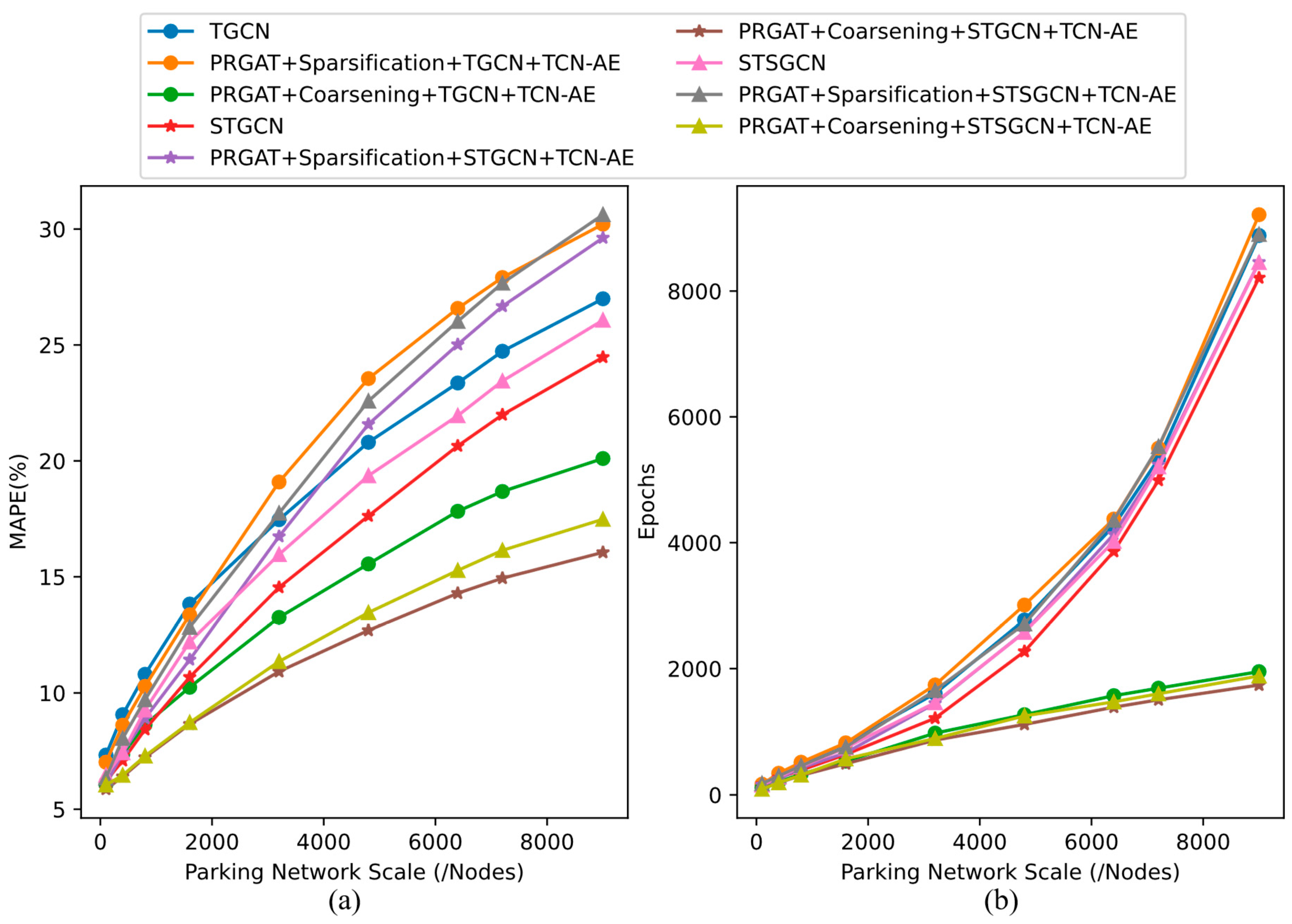
4.6. Ablation Results

To further validate the rationality of each component within the framework, we conducted an ablation study based on the task of predicting the occupancy rate of parking lots in the Bao’an District for the next 15 minutes during the evening rush hour. The ablation experiments were divided into two parts, separately assessing the impact of PRGAT and TCN-AE on three sets of baseline models, with the coarsening ratio set to 0.6 in the experiments.

Figure 8(a) shows the experimental results of parking predictions using various types of adjacency matrices. Clearly, among all baseline methods, the ParkingRank attention matrix constructed by PRGAT exhibits the best performance, achieving an average reduction in relative error of about 38.3%. PRGAT, by integrating the attention coefficient matrix with the parking spatio-temporal transition matrix, delves deep into the feature and spatial dependencies between parking lots, effectively restoring real parking demand scenarios. In contrast, traditional static adjacency matrices, built solely on spatial location information, overlook the intrinsic characteristics of parking lots and their interactions with the surrounding environment. Often, they fail to fully capture the complex interactions and dynamic changes between parking lots, limiting the authenticity and dynamism of the scenarios captured by the model, and thus performing poorly in downstream prediction tasks. Moreover, compared to the traditional GAT mechanism, another advantage of PRGAT is that it not only offers a more detailed and dynamic method to represent parking graphs, but it also intuitively reflects which parking lots have stronger comprehensive service capabilities at specific moments, thus becoming a key basis for making parking decisions.

However, a limitation of the PRGAT is that it aggregates node feature information considering only the 2nd-order neighborhood, neglecting the potential connections between distant nodes. This may lead to inadequate capturing of the interactions between remote parking lots during holidays or major events. Therefore, future research exploring and implementing graph convolutional networks that include higher-order neighborhood information will be crucial. This will enable the model to capture a broader range of node interactions, thereby enhancing the accuracy and practicality of the predictions.

Figure 8(b) illustrates the effect of the AE on the prediction framework. From the figure, it can be found that not adding the AE leads to an average decrease in prediction accuracy of about 30.1%. This is because the coarsened parking graph changes its original spatial relationship, and simply splicing a set of vertex features corresponding to each hypernode will lead to redundancy of hypernode information and dimensionality inflation, thus limiting the model’s generalization ability. In addition, the loss of the intrinsic connection between nodes will also lead to the model’s inability to fully exploit the spatial dependency of the coarsened graph. On the contrary, the approach using autoencoder can selectively extract and reconstruct the key features inside the hypernodes, thus effectively adapting to the spatial changes inside the hypernodes. Meanwhile, we additionally introduce TCN in the encoding-decoding process, which enhances the model’s ability to learn the laws behind the dynamic changes of the parking lot view from the time-series data, and is more helpful for the compression and reconstruction of the parking data, which achieves an average 20% accuracy improvement.

Figure 8. Ablation Study on Future 15-Minute Parking Prediction (a) Graph Construction (b) Autoencoder.

Figure 8. Ablation Study on Future 15-Minute Parking Prediction (a) Graph Construction (b) Autoencoder.

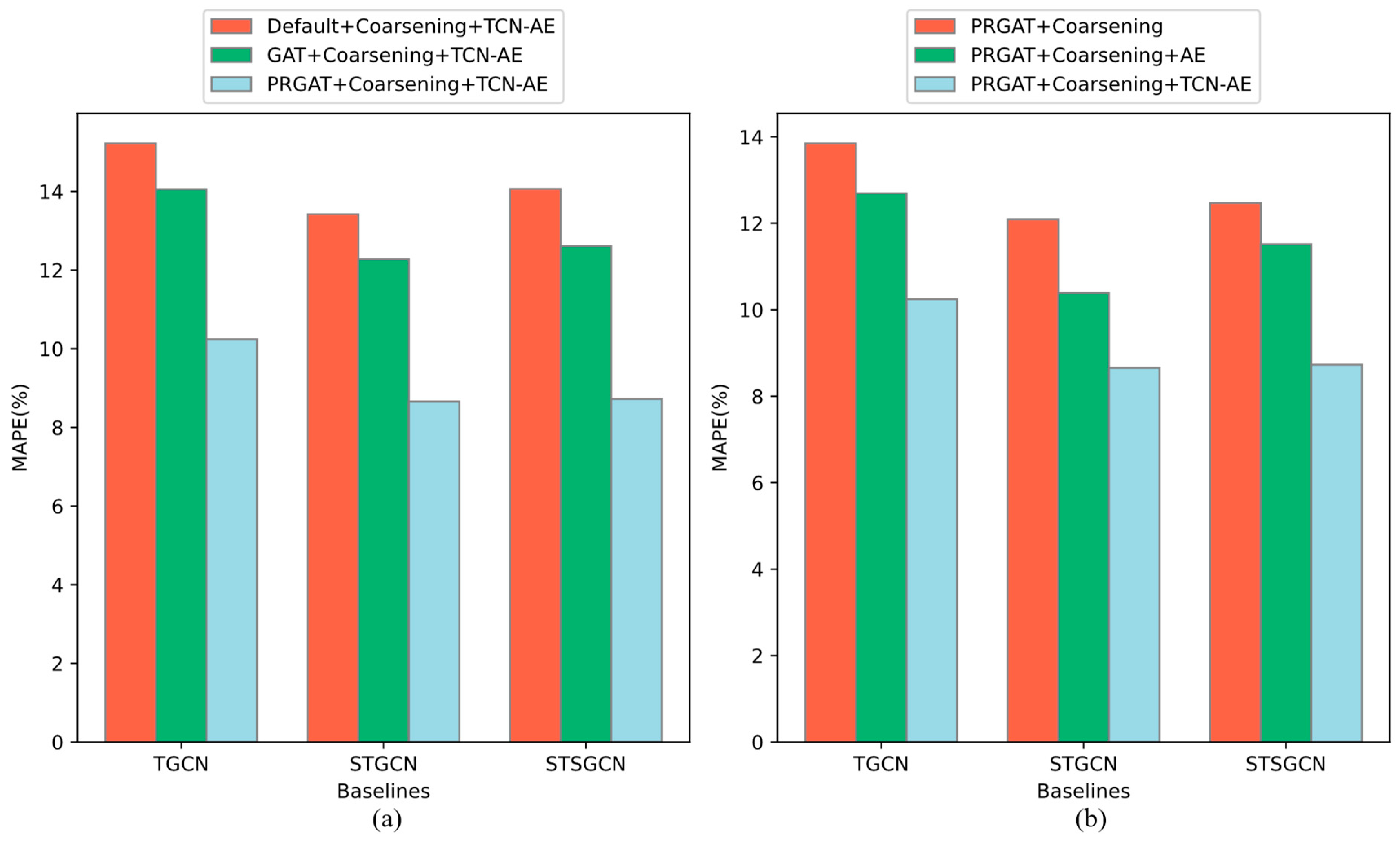
5. Conclusion

In this study, we propose an innovative large-scale urban parking prediction framework based on real-time service capabilities. Specifically, we first introduce a GAT mechanism based on real-time service capabilities, constructing a dynamic parking graph that reflects real-time parking behavior preferences. This aids spatio-temporal GCNs models in more accurately capturing the interactions and trends of change between parking lots. Subsequently, we designed a large-scale urban parking prediction framework based on coarsening and TCN-AE, aimed at effectively reducing the training time required for models to process complex parking data. Finally, we conducted experiments on a real dataset from Shenzhen’s parking lots to validate the performance of our proposed prediction framework. The experimental results show that our framework significantly improves both accuracy and efficiency compared to traditional parking prediction methods. Furthermore, as the graph scale expands, our framework’s performance exhibits even more pronounced advantages, underscoring its immense potential in addressing complex urban parking problems in practical applications.

While our research has achieved certain results, future work still needs to focus on improving and further exploring the following issues:

• Selection of Coarsening Ratio: The coarsening dimension utilized in this study was determined through experimentation with a grid search strategy, yielding a general range that may limit its applicability to the specific dataset used and not be accurate enough for others. Therefore, in our subsequent efforts, we aim to employ deep learning methods to automatically learn and ascertain the optimal coarsening dimension.
• Integration of Multi-source Data: Given that parking demand is influenced by a wide array of factors, including nearby traffic flow, weather conditions, and more, we intend to incorporate multiple data sources for feature fusion in the future. This approach will enhance the model’s comprehension of parking scenarios, providing a richer understanding of the complex dynamics at play.
• Global Information Aggregation: The PRGAT algorithm proposed in this paper aggregates node feature information considering only the 2nd-order neighborhood, thus overlooking the influence of distant global nodes. In our future research, we plan to incorporate higher-order global information by employing concepts from fractal theory.

References

- Xin, H. China registers 415 million motor vehicles, 500 million drivers. Website, 2024. https://english.www.gov.cn/archive/statistics/202212/08/content_WS6391cafcc6d0a757729e41bc.html.
- Zou, W.; Sun, Y.; Zhou, Y.; Lu, Q.; Nie, Y.; Sun, T.; Peng, L. Limited sensing and deep data mining: A new exploration of developing city-wide parking guidance systems. IEEE Intelligent Transportation Systems Magazine 2020, 14, 198–215. [Google Scholar] [CrossRef]
- Ke, R.; Zhuang, Y.; Pu, Z.; Wang, Y. A smart, efficient, and reliable parking surveillance system with edge artificial intelligence on IoT devices. IEEE Transactions on Intelligent Transportation Systems 2020, 22, 4962–4974. [Google Scholar] [CrossRef]
- Research.; ltd, M. China Smart Parking Industry Report, 2022; Research In China, 2022.
- Rizvi, S.R.; Zehra, S.; Olariu, S. Aspire: An agent-oriented smart parking recommendation system for smart cities. IEEE Intelligent Transportation Systems Magazine 2018, 11, 48–61. [Google Scholar] [CrossRef]
- Kotb, A.O.; Shen, Y.c.; Huang, Y. Smart parking guidance, monitoring and reservations: a review. IEEE Intelligent Transportation Systems Magazine 2017, 9, 6–16. [Google Scholar] [CrossRef]
- Yang, K.; Tang, X.; Qin, Y.; Huang, Y.; Wang, H.; Pu, H. Comparative study of trajectory tracking control for automated vehicles via model predictive control and robust H-infinity state feedback control. Chinese Journal of Mechanical Engineering 2021, 34, 1–14. [Google Scholar] [CrossRef]
- Tang, X.; Yang, Y.; Liu, T.; Lin, X.; Yang, K.; Li, S. Path planning and tracking control for parking via soft actor-critic under non-ideal scenarios. IEEE/CAA Journal of Automatica Sinica, 2023. [Google Scholar]
- Fan, J.; Hu, Q.; Xu, Y.; Tang, Z. Predicting vacant parking space availability: a long short-term memory approach. IEEE Intelligent Transportation Systems Magazine 2020, 14, 129–143. [Google Scholar] [CrossRef]
- Lin, T.; Rivano, H.; Le Mouël, F. A survey of smart parking solutions. IEEE Transactions on Intelligent Transportation Systems 2017, 18, 3229–3253. [Google Scholar] [CrossRef]
- Anand, D.; Singh, A.; Alsubhi, K.; Goyal, N.; Abdrabou, A.; Vidyarthi, A.; Rodrigues, J.J. A smart cloud and IoVT-based kernel adaptive filtering framework for parking prediction. IEEE Transactions on Intelligent Transportation Systems 2022, 24, 2737–2745. [Google Scholar] [CrossRef]
- Ku, Y.; Guo, C.; Zhang, K.; Cui, Y.; Shu, H.; Yang, Y.; Peng, L. Toward Directed Spatiotemporal Graph: A New Idea for Heterogeneous Traffic Prediction. IEEE Intelligent Transportation Systems Magazine 2024, 16, 70–87. [Google Scholar] [CrossRef]
- Li, J.; Qu, H.; You, L. An integrated approach for the near real-time parking occupancy prediction. IEEE Transactions on Intelligent Transportation Systems 2022, 24, 3769–3778. [Google Scholar] [CrossRef]
- Shuai, C.; Zhang, X.; Wang, Y.; He, M.; Yang, F.; Xu, G. Online car-hailing origin-destination forecast based on a temporal graph convolutional network. IEEE Intelligent Transportation Systems Magazine 2023. [Google Scholar] [CrossRef]
- Li, D.; Wang, J. A Fusion Deep Learning Model via Sequence-to-Sequence Structure for Multiple-Road-Segment Spot Speed Prediction. IEEE Intelligent Transportation Systems Magazine 2022, 15, 230–243. [Google Scholar] [CrossRef]
- Zhang, J.; Chen, Z.; Xu, Z.; Du, M.; Yang, W.; Guo, L. A distributed collaborative urban traffic big data system based on cloud computing. IEEE Intelligent Transportation Systems Magazine 2018, 11, 37–47. [Google Scholar] [CrossRef]
- Zhou, X.; Zhang, Y.; Li, Z.; Wang, X.; Zhao, J.; Zhang, Z. Large-scale cellular traffic prediction based on graph convolutional networks with transfer learning. Neural Computing and Applications 2022, 1–11. [Google Scholar] [CrossRef]
- Fahrbach, M.; Goranci, G.; Peng, R.; Sachdeva, S.; Wang, C. Faster graph embeddings via coarsening. In Proceedings of the international conference on machine learning. PMLR; 2020; pp. 2953–2963. [Google Scholar]
- Cai, C.; Wang, D.; Wang, Y. Graph coarsening with neural networks. arXiv 2021, arXiv:2102.01350. [Google Scholar]
- Loukas, A. Graph reduction with spectral and cut guarantees. Journal of Machine Learning Research 2019, 20, 1–42. [Google Scholar]
- Kumar, M.; Sharma, A.; Kumar, S. A unified framework for optimization-based graph coarsening. Journal of Machine Learning Research 2023, 24, 1–50. [Google Scholar]
- Jin, Y.; Loukas, A.; JaJa, J. Graph coarsening with preserved spectral properties. In Proceedings of the International Conference on Artificial Intelligence and Statistics. PMLR, 2020, pp. 4452–4462.
- Chen, Y.; Shu, T.; Zhou, X.; Zheng, X.; Kawai, A.; Fueda, K.; Yan, Z.; Liang, W.; Kevin, I.; Wang, K. Graph attention network with spatial-temporal clustering for traffic flow forecasting in intelligent transportation system. IEEE Transactions on Intelligent Transportation Systems 2022. [Google Scholar] [CrossRef]
- Lu, Z.; Lv, W.; Xie, Z.; Du, B.; Xiong, G.; Sun, L.; Wang, H. Graph sequence neural network with an attention mechanism for traffic speed prediction. ACM Transactions on Intelligent Systems and Technology (TIST) 2022, 13, 1–24. [Google Scholar] [CrossRef]
- Lu, Q.; Tang, Z.; Nie, Y.; Peng, L. ParkingRank-D: A Spatial-temporal Ranking Model of Urban Parking Lots in City-wide Parking Guidance System. In Proceedings of the 2019 IEEE Intelligent Transportation Systems Conference (iTSC). IEEE; 2019; pp. 388–393. [Google Scholar]
- Dong, S.; Chen, M.; Peng, L.; Li, H. Parking rank: A novel method of parking lots sorting and recommendation based on public information. In Proceedings of the 2018 IEEE International Conference on Industrial Technology (ICIT). IEEE; 2018; pp. 1381–1386. [Google Scholar]
- Huang, C.J.; Ma, H.; Yin, Q.; Tang, J.F.; Dong, D.; Chen, C.; Xiang, G.Y.; Li, C.F.; Guo, G.C. Realization of a quantum autoencoder for lossless compression of quantum data. Physical Review A 2020, 102, 032412. [Google Scholar] [CrossRef]
- Liu, M.; Zhu, T.; Ye, J.; Meng, Q.; Sun, L.; Du, B. Spatio-temporal autoencoder for traffic flow prediction. IEEE Transactions on Intelligent Transportation Systems 2023. [Google Scholar] [CrossRef]
- Fainstein, F.; Catoni, J.; Elemans, C.P.; Mindlin, G.B. The reconstruction of flows from spatiotemporal data by autoencoders. Chaos, Solitons & Fractals 2023, 176, 114115. [Google Scholar]
- Guo, G.; Yuan, W.; Liu, J.; Lv, Y.; Liu, W. Traffic forecasting via dilated temporal convolution with peak-sensitive loss. IEEE Intelligent Transportation Systems Magazine 2021, 15, 48–57. [Google Scholar] [CrossRef]
- Du, W.; Li, B.; Chen, J.; Lv, Y.; Li, Y. A spatiotemporal hybrid model for airspace complexity prediction. IEEE Intelligent Transportation Systems Magazine 2022, 15, 217–224. [Google Scholar] [CrossRef]
- Yao, Z.; Xia, S.; Li, Y.; Wu, G.; Zuo, L. Transfer learning with spatial–temporal graph convolutional network for traffic prediction. IEEE Transactions on Intelligent Transportation Systems 2023. [Google Scholar] [CrossRef]
- Zhao, L.; Song, Y.; Zhang, C.; Liu, Y.; Wang, P.; Lin, T.; Deng, M.; Li, H. T-gcn: A temporal graph convolutional network for traffic prediction. IEEE transactions on intelligent transportation systems 2019, 21, 3848–3858. [Google Scholar] [CrossRef]
- Sun, Y.; Jiang, X.; Hu, Y.; Duan, F.; Guo, K.; Wang, B.; Gao, J.; Yin, B. Dual dynamic spatial-temporal graph convolution network for traffic prediction. IEEE Transactions on Intelligent Transportation Systems 2022, 23, 23680–23693. [Google Scholar] [CrossRef]
- Zheng, Y.; Li, W.; Zheng, W.; Dong, C.; Wang, S.; Chen, Q. Lane-level heterogeneous traffic flow prediction: A spatiotemporal attention-based encoder–decoder model. IEEE Intelligent Transportation Systems Magazine 2022. [Google Scholar] [CrossRef]
- Li, D.; Lasenby, J. Spatiotemporal attention-based graph convolution network for segment-level traffic prediction. IEEE Transactions on Intelligent Transportation Systems 2021, 23, 8337–8345. [Google Scholar] [CrossRef]
- Wickman, R.; Zhang, X.; Li, W. A Generic Graph Sparsification Framework using Deep Reinforcement Learning. arXiv preprint arXiv:2112.01565, arXiv:2112.01565 2021.
- Sadhanala, V.; Wang, Y.X.; Tibshirani, R. Graph sparsification approaches for laplacian smoothing. In Proceedings of the Artificial Intelligence and Statistics. PMLR; 2016; pp. 1250–1259. [Google Scholar]
- Wu, H.Y.; Chen, Y.L. Graph sparsification with generative adversarial network. In Proceedings of the 2020 IEEE International Conference on Data Mining (ICDM). IEEE; 2020; pp. 1328–1333. [Google Scholar]
- Chen, J.; Saad, Y.; Zhang, Z. Graph coarsening: from scientific computing to machine learning. SeMA Journal 2022, 79, 187–223. [Google Scholar] [CrossRef]
- Dhillon, I.S.; Guan, Y.; Kulis, B. Weighted graph cuts without eigenvectors a multilevel approach. IEEE transactions on pattern analysis and machine intelligence 2007, 29, 1944–1957. [Google Scholar] [CrossRef] [PubMed]
- Rhouma, D.; Ben Romdhane, L. An efficient multilevel scheme for coarsening large scale social networks. Applied Intelligence 2018, 48, 3557–3576. [Google Scholar] [CrossRef]
- Wang, Q.; Jiang, H.; Qiu, M.; Liu, Y.; Ye, D. Tgae: Temporal graph autoencoder for travel forecasting. IEEE Transactions on Intelligent Transportation Systems 2022. [Google Scholar] [CrossRef]
- Mo, R.; Pei, Y.; Venkatarayalu, N.V.; Joseph, P.N.; Premkumar, A.B.; Sun, S.; Foo, S.K.K. Unsupervised TCN-AE-based outlier detection for time series with seasonality and trend for cellular networks. IEEE Transactions on Wireless Communications 2022, 22, 3114–3127. [Google Scholar] [CrossRef]
- Veličković, P.; Cucurull, G.; Casanova, A.; Romero, A.; Lio, P.; Bengio, Y. Graph attention networks. arXiv 2017, arXiv:1710.10903. [Google Scholar]
- Yu, B.; Yin, H.; Zhu, Z. Spatio-temporal graph convolutional networks: A deep learning framework for traffic forecasting. arXiv 2017, arXiv:1709.04875. [Google Scholar]
- Song, C.; Lin, Y.; Guo, S.; Wan, H. Spatial-temporal synchronous graph convolutional networks: A new framework for spatial-temporal network data forecasting. In Proceedings of the Proceedings of the AAAI conference on artificial intelligence, 2020, Vol.; 2020; Volume 34, pp. 914–921. [Google Scholar]
- Wang, Y.; Ku, Y.; Liu, Q.; Yang, Y.; Peng, L. Large-Scale Parking Data Prediction: From A Graph Coarsening Perspective. In Proceedings of the 2023 IEEE 26th International Conference on Intelligent Transportation Systems (ITSC). IEEE; 2023; pp. 1410–1415. [Google Scholar]