Designing a Holistic Student Evaluation Model for E-Learning Using a Multi-Task Attention-Based Deep Learning Approach

This study presents the development and evaluation of a Multi-Task Long Short-Term Memory (LSTM) model with an Attention Mechanism designed to predict students' academic performance. The model concurrently addresses two tasks: predicting overall performance (total score) as a regression task and categorizing performance levels (remarks) as a classification task. By processing both tasks simultaneously, the model optimizes computational efficiency and resource use. The dataset includes detailed student performance records across various metrics such as Continuous Assessment, Practical Skills, Demeanor, Presentation Quality, Attendance, and Participation. The model's performance was evaluated using comprehensive metrics. For the regression task, it achieved a Mean Absolute Error (MAE) of 0.0249, Mean Squared Error (MSE) of 0.0012, and Root Mean Squared Error (RMSE) of 0.0346. For the classification task, it attained perfect scores with an accuracy, precision, recall, and F1 score of 1.0. These results highlight the model's high accuracy and robustness in predicting both continuous and categorical outcomes. The Attention Mechanism enhances the model's capabilities by identifying and focusing on the most relevant features. This study demonstrates the effectiveness of the Multi-Task LSTM with Attention Mechanism in educational data analysis, offering a reliable tool for predicting student performance and potential broader applications in similar multi-task learning contexts. Future work will explore further enhancements and wider applications to improve predictive accuracy and efficiency.

Keywords:

Subject: Computer Science and Mathematics - Artificial Intelligence and Machine Learning

1. Introduction

Traditional student evaluation practices offer valuable insights into academic achievement and learning progress, providing a structured means to measure how well students understand course material and achieve learning objectives [1] These methods, such as standardized testing, summative assessments, grading, and multiple-choice tests, are designed to assess a wide range of cognitive skills, from basic recall to higher-order thinking [2]

However, despite their utility, these traditional practices have long relied on methods that are ethically and intellectually questionable [3]. A significant concern is that these practices often do not allow students to explain their answers [4]. For instance, multiple-choice tests and other standardized assessments typically offer limited opportunities for students to demonstrate their reasoning or the process by which they arrived at their answers [5]. This can lead to an incomplete understanding of a student’s true capabilities and knowledge, as these formats prioritize the final answer over the thought process.

Moreover, traditional evaluation methods frequently fail to accommodate the diverse physiological strengths and weaknesses of students [6]. Standardized tests, for instance, are often designed with a one-size-fits-all approach that does not consider individual differences in learning styles, cognitive processing speeds, or test-taking abilities [7]. Students with different learning needs, such as those with learning disabilities or attention disorders, may find these assessments particularly challenging and unreflective of their true potential [8].

Student performance accountability should not rest solely on the students themselves. Instead, assessing learning outcomes and guiding instructional practices should involve a broader range of metrics, which are often overlooked [9]. Student evaluation extends beyond mere testing and intellectual performance; it should not rely predominantly on exam scores as the primary measure of academic achievement. Although exams offer valuable insights into a student's grasp of course material, they often fall short in capturing the multifaceted nature of learning and development [10].

For physiological differences, time-honored practices often overlook the importance of providing a holistic view of student development [11]. Behavioral and practical skills, critical thinking, creativity, and collaborative abilities are crucial aspects of learning that are not adequately captured by conventional testing methods. As a result, students who excel in these areas but struggle with traditional exams may not receive the recognition they deserve for their overall capabilities and contributions [12].

Although traditional student evaluation practices provide essential insights into academic performance, their limitations in addressing ethical and intellectual concerns, along with their failure to consider the diverse needs and strengths of all students, highlight the need for a more comprehensive and inclusive approach to assessment [13]. This approach should allow for greater flexibility, accommodate individual differences, and emphasize a broader range of skills and competencies to truly reflect a student’s overall learning and development [14].

Incorporating a broader range of metrics to assess student performance such as behavioral factors, practical skills, class participation, and engagement has received some importance from researchers [15]. However it should be acknowledged as essential components of the learning process that contribute significantly to a student's overall success [16].

Despite this recognition, incorporating diverse performance metrics into a cohesive evaluation framework remains a significant challenge. Existing evaluation models often lack the flexibility to accommodate multiple types of data and struggle to provide interpretable insights into the factors driving evaluation outcomes [17]. As a result, educators face difficulty in understanding the shade of student performance and tailoring their instructional strategies accordingly [18].

To address these challenges, this study proposes the development of an innovative holistic student evaluation model for e-learning environments. This model aims to incorporate a diverse array of performance metrics, including exams, behavior assessments, practical assignments, presentations, class attendance, participation, and continuous assessments. By leveraging advanced deep learning techniques, such as LSTM-based multi-task learning and attention mechanisms, the proposed model seeks to capture the complex relationships among various evaluation metrics, providing a more comprehensive understanding of student performance.

2. Literature

The integration of technology in education has transformed the landscape of teaching and learning, leading to the emergence of innovative approaches to student assessment, prediction, and recommendation. As digital platforms become increasingly prevalent in educational settings, researchers are exploring novel methods to enhance learning outcomes, personalize instruction, and improve student engagement. This literature review examines recent studies that investigate various aspects of e-learning, including cognitive classification of text, prediction of student behavior, performance analysis, and course recommendation. Recently, [19] focuses on the cognitive classification of text in e-learning materials, employing Bloom’s taxonomy as a framework. The study introduces MTBERT-Attention, a model combining multi-task learning (MTL), BERT, and a co-attention mechanism to enhance generalization capacity and data augmentation. Comprehensive testing demonstrates the model's superior performance and explainability compared to baseline models. Furthermore, [20] address the prediction of student behavior in e-learning environments. They propose a variant of Long-Short Term Memory (LSTM) and a soft-attention mechanism to model heterogeneous behaviors and make multiple predictions simultaneously. Experimental results validate the effectiveness of the proposed model in predicting student behaviors and improving academic outcomes. Additionally, [21] focuses on predicting student performance in online education using demographic data and clickstream interactions. The study introduces an Attention-based Multi-layer LSTM (AML) model, which combines demographic and clickstream data for comprehensive analysis. Experimental results demonstrate improved prediction accuracy and F1 score compared to baseline methods.

[22] explore Knowledge Tracing (KT) in e-learning platforms, proposing Multi-task Attentive Knowledge Tracing (MAKT) to improve prediction accuracy. The study introduces Bi-task Attentive Knowledge Tracing (BAKT) and Tri-task Attentive Knowledge Tracing (TAKT) models, which jointly learn hint-taking, attempt-making, and response prediction tasks. Experimental results show that MAKT outperforms existing KT methods, indicating promising applications of multi-task learning in KT. And more recently, [23] investigated cross-type recommendation in Self-Directed Learning Systems (SDLS), proposing the Multi-task Information Enhancement Recommendation (MIER) Model. The study integrates resource representation and recommendation tasks using an attention mechanism and knowledge graph. Experimental results demonstrate the superior performance of the MIER model in predicting concepts and recommending exercises compared to existing methods. [24] focus on course recommendation in online education platforms, proposing a deep course recommendation model with multimodal feature extraction. The study utilizes LSTM and Attention mechanisms to fuse course video, audio, and textual data, supplemented with user demographic information and feedback. Experimental results show that the proposed model achieves significantly higher AUC scores compared to similar algorithms, providing accurate course recommendations for users.

Conclusively, the current literature on e-learning reveals significant gaps that justify the need for designing a holistic student evaluation model using an LSTM multi-task attention-based deep learning approach. Existing studies predominantly focus on isolated aspects of e-learning, such as cognitive classification, behavior prediction, performance analysis, and course recommendation, without integrating multiple performance metrics for a comprehensive evaluation. There is also a lack of interdisciplinary integration of advanced techniques like multi-task learning and attention mechanisms, which could enhance model robustness. A holistic evaluation model that incorporates these aspects would significantly improve the effectiveness and user experience of e-learning platforms.

3. Materials and Methods

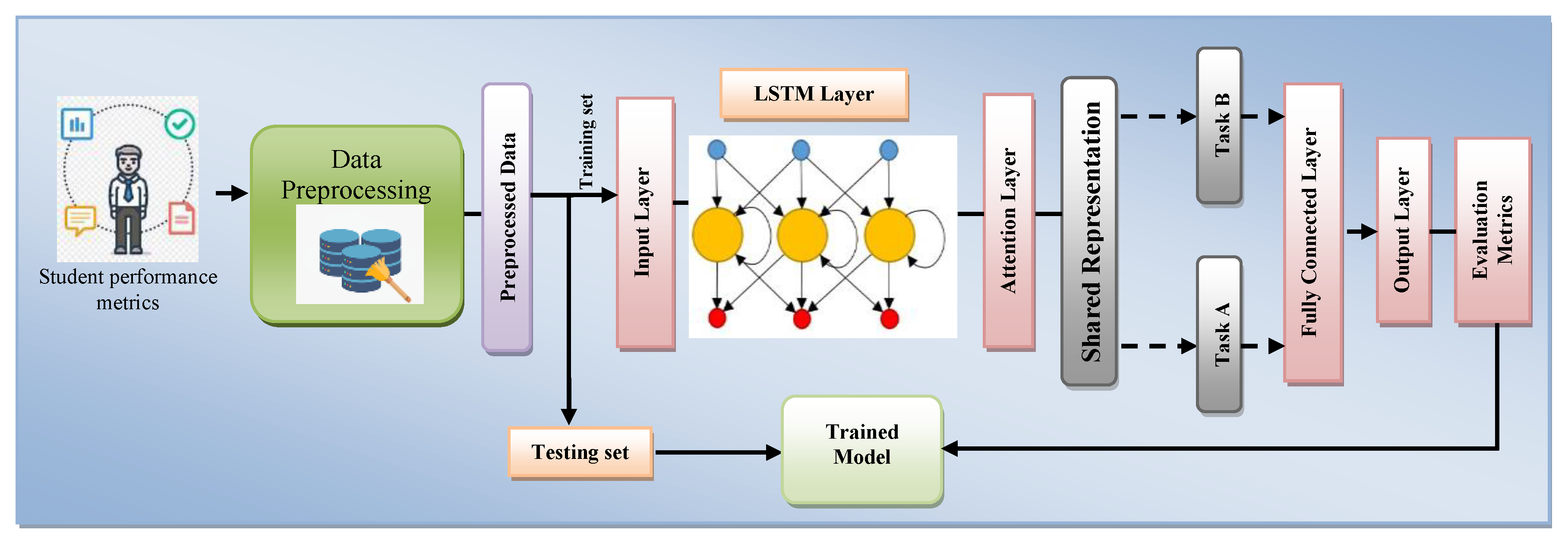
3.1. Proposed Architecture

Figure 1 illustrates the architectural framework for the Multi-Task LSTM with Attention Mechanism (MLSTM-AM) model for accurate prediction of students’ academic performance.

The proposed framework depicts the different components of the model starting with the dataset, data pre-processing, model design and training, and validation.

3.2. Dataset Creation

The typical student performance dataset traditionally revolves around two key variables: Continuous Assessment (CA) and Examination (Exam) scores. These metrics have long been the sole basis for evaluating student’s academic achievement. However, this research introduces a paradigm shift by expanding the dimensions of this performance evaluation framework. By integrating additional variables such as Attendance, Demeanor, Practical skills, Class Participation, and Presentation quality, this study pioneers a more comprehensive approach to assessing student success.

Since the dataset needed for this kind of new model is not readily available anywhere, hence the need to create a new dataset that captures the above mentioned variables. To achieve this, a suitable mathematical formulation was utilized which was then translated into a computer algorithm for creating such a higher dimensional dataset as shown in this section.

Let x1, x2, x3, ...,, x7 be Attendance, Practical, Demeanour, Presentation, Participation in class, Continuous Assessment, and Examination, respectively. Where x1, x2, x3, ..., x6 can take on 10 distinct values (i.e, 10 marks each) while x7 can take on 40 distinct values (i.e, 40 marks only). However, the summation of the values of all these variables can not be greater than 100, as the case may be.

i.e.

s c o r e = x_{1} + x_{2} + x_{3} + x_{4} + x_{5} + x_{6} + x_{7}

s c o r e = \sum_{i = 1}^{n} x_{i} v i = 1,2, \dots, n a n d n = 7

i . e, s c o r e \leq 100

To find the total number of combinations, multiply the number of possibilities for each variable:

Total combinations = (Number of possibilities for x1) x (Number of possibilities for x2) x (Number of possibilities for x3) x (Number of possibilities for x4) x (Number of possibilities for x5) x (Number of possibilities for x6) x (Number of possibilities for x7)

= 10 x 10 x 10 x 10 x 10 x 10 x 40
= 1, 000, 000 x 40
= 40, 000, 000

So, the total number of combinations is 40, 000, 000. In other words, the total number of data points would be 40, 000, 000 i.e. the new dataset containing all the above features would have 40, 000, 000 records, which is enough to train the proposed model. This formulation was implemented in python and the code snippet is displayed in Algorithm 1.

Algorithm 1: Pseudocode for data pre-processing

import itertools
import csv
# Define the range of values for each variable
range_values = range(11) # For x1 to x6
range_x7 = range(41) # For x7
# Generate all combinations of the variables
combinations = list(itertools.product(range_values, repeat=6)) # For x1 to x6
combinations_with_x7 = [(c + (x7,)) for c in combinations for x7 in range_x7] # Combine with x7
# Calculate total for each combination
combinations_with_total = [(c + (sum(c),)) for c in combinations_with_x7]
# Specify the file name
file_name = "resultPredictionDataset.csv"
# Write combinations with sum to CSV file
with open(file_name, 'w', newline='') as csvfile:
csvwriter = csv.writer(csvfile)
# Write header row
csvwriter.writerow(["x1", "x2", "x3", "x4", "x5", "x6", "x7", "total"])
# Write data rows
csvwriter.writerows(combinations_with_total)
print(f"Final Dataset Generated Successfully to {file_name}")
# total_rows = 5**6 * 70
# print("Total number of rows:", total_rows)

3.2.1. Dataset Description

The dataset generated by Algorithm, which has been published in kaggle repository () contains a collection of 40,000,000 records, each detailing various aspects important for evaluating student academic performance. These records include Continuous Assessment (CA), Practical skills proficiency, Demeanor, Presentation quality, Attendance records, Participation in class, and Examination results. The final two columns represent the overall performance (total score) and the performance class (remarks), which ranges from 1 to 5, indicating different levels of student achievement.

To provide clarity and facilitate analysis, each feature is assigned a corresponding variable: X1 corresponds to CA, X2 corresponds to Practical proficiency, X3 corresponds to Demeanor, X4 corresponds to Presentation quality, X5 corresponds to Attendance, X6 corresponds to Participation in class, and finally, X7 corresponds to Examination results. This structured framework not only simplifies data interpretation but also lays the groundwork for comprehensive analysis and insights into student academic performance.

The CA variable evaluates ongoing performance through assignments, quizzes, and tests, providing insight into consistent engagement and mastery of material. The Practical variable assesses hands-on proficiency in applying theoretical knowledge through lab work and projects. Demeanor focuses on punctuality, attentiveness, and overall conduct, reflecting social and emotional intelligence. Presentation quality is evaluated through the clarity and effectiveness of student presentations, highlighting communication skills. Attendance records quantify commitment and consistency in attending classes. Participation in class measures active engagement and contribution during discussions and activities. Together, these variables offer a comprehensive framework for assessing student strengths, areas for improvement, and overall academic progress. Table 1 presents the structure of the dataset generated in this research.

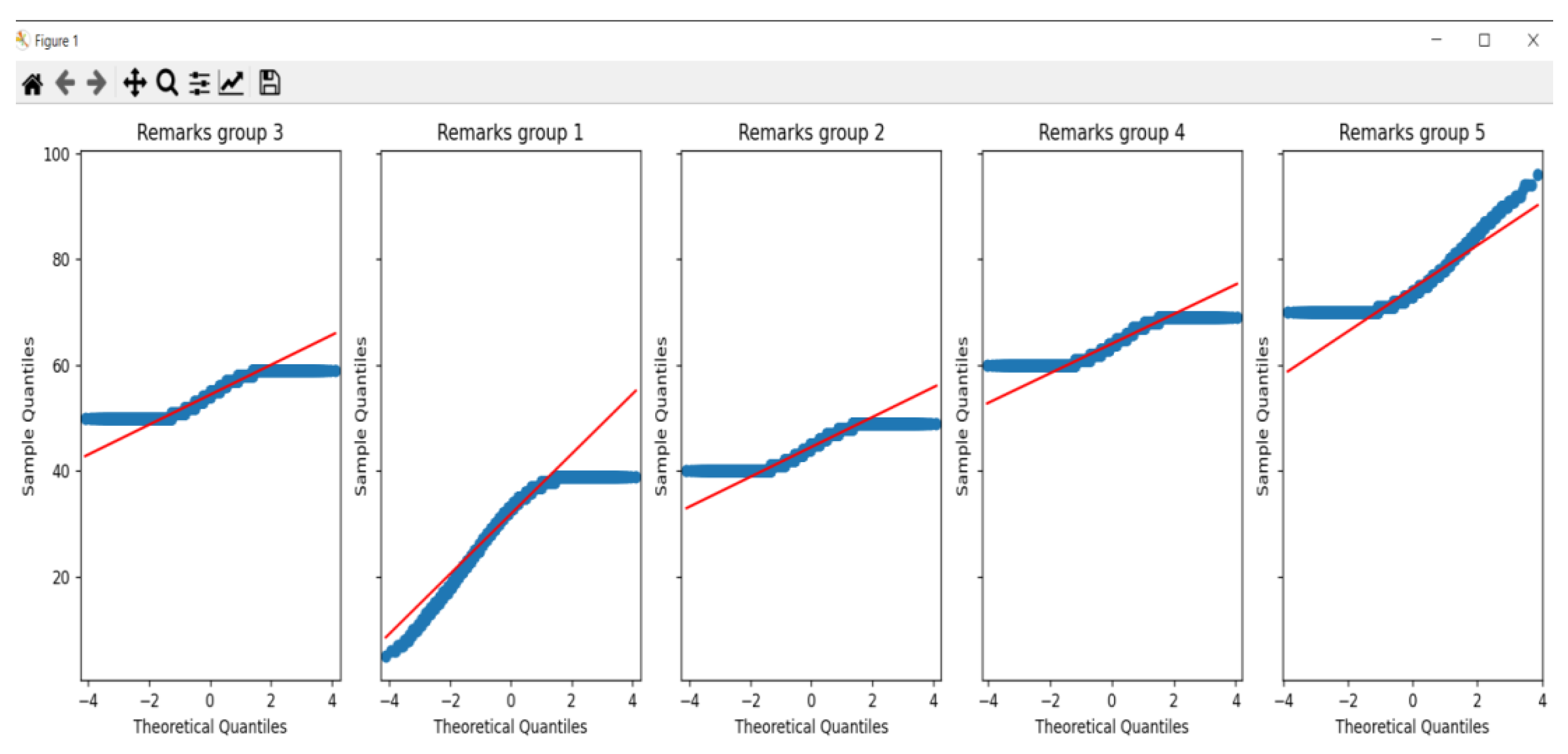
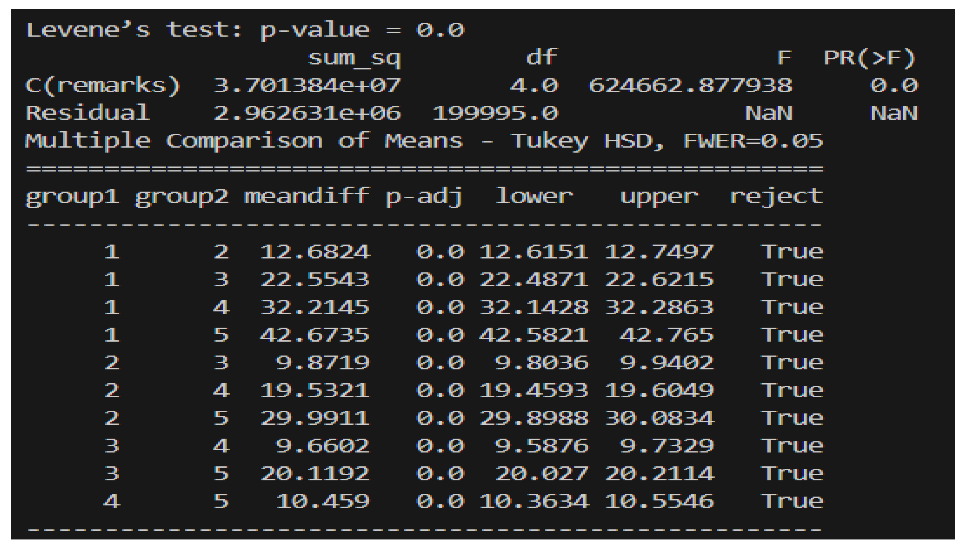
3.2.2. Data Analysis

Given the generated dataset, this study aims to explore the differences in student performance across various classes. To achieve this, an Analysis of Variance (ANOVA) was employed to determine if there are statistically significant differences in the performance scores among the different classes. To ensure the validity of the ANOVA results, normality was first checked using Q-Q plots, shown in Figure 2, and homogeneity of variance was assessed using Levene's test as depicted in Figure 3.

The Q-Q plots indicated that the normality assumption was reasonably met, while Levene’s test revealed a p-value of 0.0, indicating significant differences in variances across groups.

As shown in Figure 3, the analysis of variance (ANOVA) performed on the dataset revealed significant differences in student performance across different classes. Levene’s test for homogeneity of variances produced a p-value of 0.0, indicating that the variances among the groups are significantly different. Although this result suggests a violation of the homogeneity of variance assumption, it is expected given the context of the dataset, which comprises different classes of student performance.

The ANOVA results further support the presence of significant differences between groups. The F-statistic was calculated to be 624,662.88 with a corresponding p-value of 0.0. This extremely low p-value allows us to reject the null hypothesis and conclude that there are significant differences in the mean performance scores among the different classes of students as expected in this context.

Following the ANOVA, Tukey’s HSD post-hoc test was conducted to identify which specific groups differed significantly from each other. The results showed that all pairwise comparisons between the groups were significant, with each group displaying a mean difference that was statistically significant (p-adj < 0.05) as expected. This indicates that the performance of students in each class is distinctively different from the others.

To sum up, the analysis demonstrates clear and significant differences in student performance across different classes. Although the homogeneity of variance assumption was not met, the context of varying student performance classes justifies these significant differences. The results align with expectations and provide a robust indication of distinct performance levels among the different classes.

3.2.3. Data Preprocessing

As illustrated in Algorithm 2, the dataset is first loaded from a CSV file, ensuring that all subsequent operations are based on the complete data set. Following this, relevant features and target variables are extracted. The features include various metrics such as `x1`, `x2`, `x3`, `x4`, `x5`, `x6`, and `x7`, while the target variables consist of the `total` score and `remarks`. The `remarks` target variable is adjusted to zero-based indexing in order to align the target values with typical numerical representations used in model training. The feature set is then reshaped to fit the input requirements of a Long Short-Term Memory (LSTM) network. This reshaping transforms the data into the format required for LSTM input, with dimensions corresponding to samples, timesteps, and features. Then, the dataset is divided into training and testing subsets, allowing the model to be trained on one portion of the data and evaluated on a separate, independent portion to assess its performance effectively. Finally, the input shape for the LSTM network is defined based on the reshaped data, which is important for setting up the network architecture correctly.

Algorithm 2: Data Preprocessing

dataPreprocessing(dataset)

Load the dataset from the CSV file

Extract features as X and target variables as y_total and y_remarks

Adjust y_remarks for zero-based indexing by subtracting 1

Reshape X to fit the LSTM input format (samples, timesteps, features)

Split the dataset into training and testing sets:

X_train, X_test

y_total_train, y_total_test

y_remarks_train, y_remarks_test

Define the input shape for the LSTM network based on the reshaped data

end dataPreprocessing

3.2.4. The Model

The proposed model integrates a Multi-Task LSTM with an Attention Mechanism to enhance the prediction of students' academic performance. As detailed in Table 3, the model addresses two dependent variables: the total and remarks variables. Predicting the total variable is a regression task, while predicting the remarks variable is a classification task. Traditionally, handling these tasks would involve splitting the dataset into two and training them separately, which is time-consuming and resource-intensive. Therefore, a Multi-Task LSTM is employed to manage both tasks concurrently. Additionally, the Attention Mechanism is utilized to identify and extract the most relevant features from the dataset for the Multi-Task LSTM model. The integration of these models is mathematically presented in this section.

For a sequence S =[s₁, s₂, …, s_T] with input features s_t ϵ R^d, the LSTM layer computes forget gate, input gate, cell state update, cell state, output gate and hidden state as illustrated in equations 1 through 6, respectively.

f_{G} = S A F (W_{f} * [h_{t - 1}, n_{t}] + b_{f})

(1)

i_{G} = S A F (W_{i} * [h_{t - 1}, n_{t}] + b_{i})

(2)

Z_{t} = t a n h (W_{z} * [h_{t - 1}, n_{t}] + b_{z})

(3)

C_{t} = f_{G} * C_{t - 1} + i g * Z_{t}

(4)

o_{G} = S A F (W_{o} * [h_{t - 1}, n_{t}] + b_{o})

(5)

h_{G} = o_{G} * t a n h (C_{t})

(6)

Where SAF is the Sigmoid Activation Function, tanh is the hyperbolic tangent function, and W and b are the weights and biases.

Likewise, for a sequence H = [h₁, h₂,…, h_T], the attention mechanism calculates a context vector C_t as a weighted sum of the input sequences as shown in equation 7.

C_{t} = \sum_{t = 1}^{T} A_{t} * h_{t}

(7)

Attention score (A_t) is computed as depicted in equation 8.

A_{t} = \frac{e x p (e_{t})}{\sum_{j = 1}^{T} e x p (e_{j})}

(8)

Where e_t = score (h_t, h_t-1) = LeakyReLU(W_a * [h_t, h_t-1] + b_a).

For the regression task, the output denoted by y_t is given in equation (9).

y_{t} = W_{r} * h_{r} + b_{r}

(9)

where the hidden layer is computed as in equation (10).

h_{r} = R e L U (W_{r h} * h + b_{r h})

(10)

where W and b are weights and biases.

Also, for the classification task, the output layer denoted by y_o is given in equation (11).

y_{o} = s o f t m a x (W_{o} * h_{o} + b_{o})

(11)

where the hidden layer is computed as in equation (12).

h_{c} = R e L U (W_{c} * h + b_{c})

(12)

where W and b are weights and biases, and softmax is the activation function that outputs probabilities. Therefore, the integration is modeled as in equations 13 through 16.

L S T M L a y e r O u t p u t : H = L S T M (X)

(13)

A t t e n t i o n O u t p u t : c = A t t e n t i o n (H)

(14)

R e g r e s s i o n O u t p u t : y_{t o t a l} = W_{o} * R e L U (W_{r} * H + b_{o}) + b_{r}

(15)

C l a s s i f i c a t i o n O u t p u t : y_{c l a s s} = W_{o} * {s o f t m a x (W_{o} * R e L U (W}_{c} . H + b_{c}) + b_{o}

(16)

Where H is the output sequence from the LSTM layer, and W, b are the respective weights and biases for each task.

Then, both regression and classification losses are computed as illustrated in equations 17 and 18 respectively.

R e g r e s s i o n L o s s : {L o s s}_{r e g} = \frac{1}{N} \sum_{i = 1}^{N} {(y_{t o t a l} - {\dot{y}}_{t o t a l})}^{2}

(17)

C l a s s i f i c a t i o n L o s s : {L o s s}_{c l a s s} = - \frac{1}{N} \sum_{i = 1}^{N} y_{c l a s s} l o g ({\dot{y}}_{c l a s s})

(18)

Where

\dot{y}

denotes the predicted values.

4. Results and Discussions

This section presents the results and findings of the experimental study focused on developing a Multi-Task LSTM with an Attention Mechanism for predicting students’ academic performance conducted in this research.

4.1. Performance Evaluation Metrics

The performance of the proposed model is assessed using a variety of metrics tailored to both the regression and classification tasks. These metrics offer a detailed evaluation of the model's effectiveness in predicting students' academic performance.

For the regression task, which involves predicting the `total` variable, three primary metrics are employed. The Mean Absolute Error (MAE) measures the average magnitude of errors in the predictions, indicating how closely the predicted values align with the actual values. The MAE for the regression task is 0.0249, reflecting a low average prediction error. The Mean Squared Error (MSE) calculates the average of the squared differences between predicted and actual values, with a value of 0.0012. This metric penalizes larger errors more significantly and indicates that the model maintains a low average squared error. Additionally, the Root Mean Squared Error (RMSE) provides a measure of the average magnitude of prediction errors in the same units as the target variable. With an RMSE of 0.0346, the model demonstrates a minimal average prediction error, underscoring its regression accuracy.

For the classification task, which involves predicting the `remarks` variable, several performance metrics are considered. Accuracy measures the proportion of correctly classified instances out of the total instances, and the model achieves a perfect accuracy of 1.0, signifying flawless classification performance. Precision reflects the proportion of true positive predictions among all positive predictions made by the model, and a precision of 1.0 indicates that every positive classification was correct. Recall, which measures the proportion of actual positive instances correctly identified by the model, also achieves a perfect score of 1.0, demonstrating the model's ability to identify all actual positive instances. Finally, the F1 Score, the harmonic mean of precision and recall, balances these two aspects of classification performance. An F1 Score of 1.0 highlights the model's ideal precision and recall, illustrating its overall effectiveness in classification. The visual depiction of the model’s performance metrics is illustrated in Figure 4.

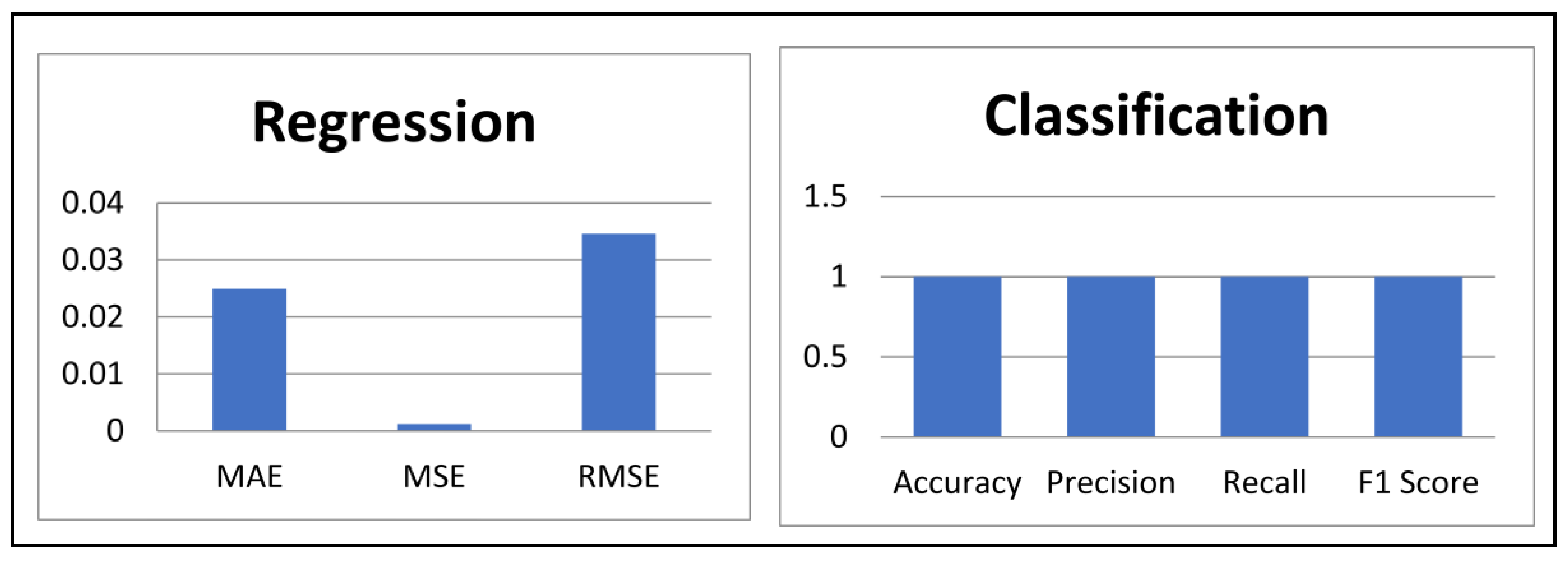
4.2. Training and Evaluation Results

To further evaluate the model’s performance, both the training and evaluation accuracies and losses were plotted for visualization as presented in Figure 5.

Over the course of 50 epochs, the training and validation metrics of the MLSTM-AM model demonstrated substantial improvement. The training and validation process of the proposed model demonstrates its robust performance in both regression and classification tasks. For the regression task, the model achieved a Mean Absolute Error (MAE) of 0.0249, indicating a low average magnitude of prediction errors, while the Mean Squared Error (MSE) of 0.0012 and the Root Mean Squared Error (RMSE) of 0.0346 further confirm the model's precision, with minimal differences between predicted and actual values. These metrics collectively highlight the model's capability to accurately predict continuous outcomes, ensuring reliable performance in the regression task.

For the classification task, the model exhibits exceptional accuracy, precision, recall, and F1 score, all achieving a perfect value of 1.0. This indicates that the model correctly classifies all instances without any errors. The high classification accuracy reflects the model's ability to distinguish between different classes effectively, while the precision and recall values demonstrate its proficiency in identifying true positives and minimizing false positives and negatives. The perfect F1 score balances these metrics, reinforcing the model's overall robustness in handling classification tasks. These results show the effectiveness of the training and validation process, ensuring the model's reliability and accuracy in predicting both continuous and categorical outcomes.

4.3. Comparative Analysis

As illustrated in Table 2, this section presents the comparison of the performance of the proposed model (MLSTM-AM) with several other recent e-learning studies. The comparison is based on Focus Area, Techniques Used, Metrics, and Gaps Addressed since they were all trained on the different dataset and performance metrics. The comparison models shown in Table 2 show several significant improvements. Existing models such as Sebbaq's MTBERT-Attention, Liu et al. best model and the setting Xie et al. Multi-task Attentive Knowledge Tracing (Su et al.'s MIER Model, and Ren et al. deep recommendation model offers insights significantly in their respective area, they emphases on particular text classification or behavior prediction or course recommendations but neither leverages multiple performance metrics at once.

The proposed model eliminates the shortfalls by employing an LSTM-based multi-task learning technique, encroached upon with attention mechanisms to offer a more in-depth analysis of student achievement. It integrates various metrics, offers real-time feedback, and demonstrates high precision in both regression and classification tasks, thereby enhancing overall student evaluation in e-learning environments.

5. Conclusion

In this study, a Multi-Task LSTM model with an Attention Mechanism was proposed to predict student academic performance effectively. The model addressed both regression and classification tasks, predicting the `total` score as a continuous variable and the `remarks` as a categorical variable. This approach allowed for efficient use of computational resources and time by handling both tasks concurrently.

The performance metrics demonstrated the model's high accuracy and low error rates. For the regression task, the model achieved a Mean Absolute Error (MAE) of 0.0249, a Mean Squared Error (MSE) of 0.0012, and a Root Mean Squared Error (RMSE) of 0.0346, indicating precise and reliable predictions. For the classification task, the model reached perfect scores across all metrics, with an accuracy, precision, recall, and F1 score of 1.0. These results highlight the model's robustness and effectiveness in both predicting continuous outcomes and classifying categorical data.

Overall, the integration of Multi-Task LSTM and Attention Mechanism proved to be a powerful approach for predicting student performance. The model's ability to accurately predict both types of outcomes showcases its potential for broader applications in educational data analysis and other fields requiring multi-task learning capabilities. Future work could explore further enhancements and applications of this model to continue improving predictive accuracy and efficiency in diverse contexts.

Author Contributions

Conceptualization, Deborah Olaniyan and Julius Olaniyan; methodology, Deborah Olaniyan and Julius Olaniyan; software, Julius Olaniyan; validation, Ibidun. C. Obagbuwa, Deborah Olaniyan. and Julius Olaniyan; formal analysis, Olorunfemi Paul Bernard.; investigation, Olorunfemi Paul Bernard.; resources, Olorunfemi Paul Bernard.; data curation, Julius Olaniyan.; writing—original draft preparation, Deborah Olaniyan.; writing—review and editing, Ibidun. C. Obagbuwa.; Julius Olaniyan.; supervision, Deborah Olaniyan.; project administration, Ibidun. C. Obagbuwa.; funding acquisition, Esiefarienrhe B. Michael. All authors have read and agreed to the published version of the manuscript.

Funding

Please add: “This research received no external funding” or “This research was funded by NAME OF FUNDER, grant number XXX” and “The APC was funded by XXX”. Check carefully that the details given are accurate and use the standard spelling of funding agency names at https://search.crossref.org/funding. Any errors may affect your future funding.

Acknowledgments

The acknowledgment section in this research paper expresses gratitude to various individuals and entities whose contributions were vital to the study's completion.

References

Suskie: L. (2018). Assessing student learning: A common sense guide. John Wiley & Sons.
Scully, D. (2019). Constructing multiple-choice items to measure higher-order thinking. Practical Assessment, Research, and Evaluation, 22(1), 4.
Morley, J., Floridi, L., Kinsey, L., & Elhalal, A. (2020). From what to how: an initial review of publicly available AI ethics tools, methods and research to translate principles into practices. Science and engineering ethics, 26(4), 2141-2168. [CrossRef]
Wei, L. (2024). Transformative pedagogy for inclusion and social justice through translanguaging, co-learning, and transpositioning. Language Teaching, 57(2), 203-214.
Say, R., Visentin, D., Saunders, A., Atherton, I., Carr, A., & King, C. (2024). Where less is more: Limited feedback in formative online multiple-choice tests improves student self-regulation. Journal of Computer Assisted Learning, 40(1), 89-103. [CrossRef]
Li, S., Zhang, X., Li, Y., Gao, W., Xiao, F., & Xu, Y. (2023). A comprehensive review of impact assessment of indoor thermal environment on work and cognitive performance-Combined physiological measurements and machine learning. Journal of Building Engineering, 106417. [CrossRef]
Ramsey, M. C., & Bowling, N. A. (2024). Building a bigger toolbox: The construct validity of existing and proposed measures of careless responding to cognitive ability tests. Organizational Research Methods, 10944281231223127. [CrossRef]
Maki, P. L. (2023). Assessing for learning: Building a sustainable commitment across the institution. Routledge.
Geletu, G. M., & Mihiretie, D. M. (2023). Professional accountability and responsibility of learning communities of practice in professional development versus curriculum practice in classrooms: Possibilities and pathways. International Journal of Educational Research Open, 4, 100223. [CrossRef]
Mohan, R. (2023). Measurement, evaluation and assessment in education. PHI Learning Pvt. Ltd.
Yuksel, P., & Bailey, J. (2024). Designing a Holistic Syllabus: A Blueprint for Student Motivation, Learning Efficacy, and Mental Health Engagement. In Innovative Instructional Design Methods and Tools for Improved Teaching (pp. 92-108). IGI Global. [CrossRef]
Thornhill-Miller, B., Camarda, A., Mercier, M., Burkhardt, J. M., Morisseau, T., Bourgeois-Bougrine, S., ... & Lubart, T. (2023). Creativity, critical thinking, communication, and collaboration: assessment, certification, and promotion of 21st century skills for the future of work and education. Journal of Intelligence, 11(3), 54. [CrossRef]
Zughoul, O., Momani, F., Almasri, O. H., Zaidan, A. A., Zaidan, B. B., Alsalem, M. A., ... & Hashim, M. (2018). Comprehensive insights into the criteria of student performance in various educational domains. IEEE access, 6, 73245-73264. [CrossRef]
AlAfnan, M. A., & Dishari, S. (2024). ESD goals and soft skills competencies through constructivist approaches to teaching: an integrative review. Journal of Education and Learning (EduLearn), 18(3), 708-718. [CrossRef]
Wong, Z. Y., & Liem, G. A. D. (2022). Student engagement: Current state of the construct, conceptual refinement, and future research directions. Educational Psychology Review, 34(1), 107-138. [CrossRef]
Al-Adwan, A. S., Albelbisi, N. A., Hujran, O., Al-Rahmi, W. M., & Alkhalifah, A. (2021). Developing a holistic success model for sustainable e-learning: A structural equation modeling approach. Sustainability, 13(16), 9453. [CrossRef]
Zaffar, M., Garg, S., Milford, M., Kooij, J., Flynn, D., McDonald-Maier, K., & Ehsan, S. (2021). Vpr-bench: An open-source visual place recognition evaluation framework with quantifiable viewpoint and appearance change. International Journal of Computer Vision, 129(7), 2136-2174. [CrossRef]
Goodwin, B., Rouleau, K., Abla, C., Baptiste, K., Gibson, T., & Kimball, M. (2022). The new classroom instruction that works: The best research-based strategies for increasing student achievement. ASCD.
Sebbaq, H. (2023). MTBERT-Attention: An Explainable BERT Model based on Multi-Task Learning for Cognitive Text Classification. Scientific African, 21, e01799. [CrossRef]
Liu, H., Zhu, Y., Zang, T., Xu, Y., Yu, J., & Tang, F. (2021). Jointly modeling heterogeneous student behaviors and interactions among multiple prediction tasks. ACM Transactions on Knowledge Discovery from Data (TKDD), 16(1), 1-24. [CrossRef]
Xie, Y. (2021). Student performance prediction via attention-based multi-layer long-short term memory. Journal of Computer and Communications, 9(8), 61-79. [CrossRef]
He, L., Li, X., Wang, P., Tang, J., & Wang, T. (2023). Integrating fine-grained attention into multi-task learning for knowledge tracing. World Wide Web, 26(5), 3347-3372. [CrossRef]
Su, Y., Yang, X., Lu, J., Liu, Y., Han, Z., Shen, S., ... & Liu, Q. (2024). Multi-task Information Enhancement Recommendation model for educational Self-Directed Learning System. Expert Systems with Applications, 252, 124073. [CrossRef]
Ren, X., Yang, W., Jiang, X., Jin, G., & Yu, Y. (2022). A deep learning framework for multimodal course recommendation based on LSTM+ attention. Sustainability, 14(5), 2907. [CrossRef]

Figure 1. Proposed Framework.

Figure 2. Q-Q plots.

Figure 3. Levene's test, Anova Table and Tukey's HSD test.

Figure 4. MLST-AM Performance Plot.

Figure 5. Training and Validation Accuracy and Loss.

Table 1. Dataset Sample.

x1	x2	x3	x4	x5	x6	x7	total	remarks
7	2	3	5	4	3	22	46	2
7	2	5	9	6	8	39	76	5
7	2	5	3	8	7	30	62	4
5	4	7	5	2	4	22	49	2
5	4	9	5	3	6	14	46	2
0	1	1	6	8	4	35	55	3
5	4	8	8	7	1	6	39	1
4	0	0	7	8	7	35	61	4
3	10	6	7	1	10	26	63	4
4	0	0	3	0	0	18	25	1
8	7	7	10	1	1	9	43	2
8	7	10	3	8	4	35	75	5
5	4	8	6	3	9	20	55	3
5	4	6	5	3	9	9	41	2
2	8	9	7	6	6	3	41	2
2	8	9	6	8	3	34	70	5
2	9	2	10	0	1	2	26	1

Table 2. Performance Comparison.

Author	Focus Area	Techniques Used	Metrics	Gaps	Proposed Model
Liu et al. (2021)	Prediction of student behavior	LSTM with soft-attention mechanism	Effective in predicting student behaviors and improving academic outcomes	Does not consider holistic student performance, limited to behavior prediction	Uses LSTM with multi-task learning for both regression and classification
Xie (2021)	Predicting student performance	Attention-based Multi-layer LSTM (AML)	Improved prediction accuracy and F1 score using demographic and clickstream data	Limited to performance prediction, lacks comprehensive metric integration	Combines various metrics for a complete evaluation of student performance
Ren et al. (2022)	Course recommendation	Deep course recommendation model with LSTM and Attention	Higher AUC scores in course recommendations	Focuses on course recommendations, lacks integration of diverse metrics	Integrates multimodal data for comprehensive student performance evaluation
He et al. (2023)	Knowledge Tracing (KT)	Multi-task Attentive Knowledge Tracing (MAKT)	Improved prediction accuracy in KT tasks	Focuses on KT, does not address real-time feedback or holistic evaluation	Provides real-time feedback, integrates multiple metrics for holistic evaluation
Sebbaq (2023)	Cognitive classification of text	Multi-task BERT (MTBERT-Attention) with co-attention mechanism	Superior performance and explainability in text classification	Focuses on text classification only, lacks holistic student evaluation	Integrates multiple performance metrics, captures complex relationships
Su et al. (2024)	Cross-type recommendation in SDLS	Multi-task Information Enhancement Recommendation (MIER) Model with attention and knowledge graph	Superior performance in concept prediction and exercise recommendation	Limited to recommendation systems, does not provide holistic student evaluation	Utilizes attention mechanisms for comprehensive evaluation of multiple student metrics

Disclaimer/Publisher’s Note: The statements, opinions and data contained in all publications are solely those of the individual author(s) and contributor(s) and not of MDPI and/or the editor(s). MDPI and/or the editor(s) disclaim responsibility for any injury to people or property resulting from any ideas, methods, instructions or products referred to in the content.

© 2024 by the authors. Licensee MDPI, Basel, Switzerland. This article is an open access article distributed under the terms and conditions of the Creative Commons Attribution (CC BY) license (http://creativecommons.org/licenses/by/4.0/).

Copyright: This open access article is published under a Creative Commons CC BY 4.0 license, which permit the free download, distribution, and reuse, provided that the author and preprint are cited in any reuse.

MDPI Initiatives

Important Links

Choose an area of interest and we will send you notifications of new preprints at your preferred frequency.

Disclaimer