Optimal Forest Management Using Multi-Objective and Game Theory Techniques: Considering Environmental and Economic Factors

Preprint

Article

Optimal Forest Management Using Multi-Objective and Game Theory Techniques: Considering Environmental and Economic Factors

Altmetrics

Downloads

Views

Comments

A peer-reviewed article of this preprint also exists.

Neda Amiri

Soleiman Mohammadi Limaei^*

Neda Amiri

Soleiman Mohammadi Limaei^*

This version is not peer-reviewed

Submitted:

12 September 2024

Posted:

14 September 2024

You are already at the latest version

Alerts

Abstract

The forest is a complex and dynamic ecosystem that requires integrated planning and management, considering economic, social, environmental, and ecological dimensions. Different stakeholders often have conflicting goals, making optimal management decisions challenging. This study aims to balance increasing economic benefits for forest users with reducing negative environmental impacts, aligning the interests of managers, government institutions, and policymakers. To achieve this, multi-objective optimization methods and game theory were used. The objectives were to maximize the net present value of wood harvesting and the amount of carbon sequestration. The study was conducted in the Shafarood forest in northern Iran. Data collected included stumpage prices, variable harvesting costs, tree density per ha, volume per ha, growth rates, interest rates, carbon sequestration, and labor costs. Using this data, models were developed for the expected mean price of various species, stored carbon, logistics growth, and labor. After adjusting the objective functions and model constraints, the range of Pareto optimal solutions for the multi-objective model and the Nash equilibrium for the game theory model were determined using the epsilon-constrain method. The results indicate that both modeling approaches can identify optimal points for balancing economic and environmental goals. The Pareto optimal range and Nash equilibrium allow for informed decision-making in managing the Hyrcanian forests, accommodating different user goals. Therefore, both models are effective tools for forest management planning and provide a framework for achieving sustainable management practices.

Keywords:

Subject: Biology and Life Sciences - Forestry

1. Introduction

Forest ecosystems provide numerous services that are essential for human well-being and welfare, characterized by intricate interconnections among forest ecosystem services (FESs) [1]. Implementing sustainable forest management (SFM) policies demands an understanding of the trade-offs, conflicts, and synergies among key forest ecosystem services (FESs), highlighting the need for decision-support tools that can address multiple objectives [2,3].

The complex and heterogeneous nature of forest ecosystems has consistently presented challenges for effective forest planning and management. This has prompted researchers to seek optimal strategies for forest management. Optimization in this context may involve presenting general or specific solutions, expressed through numerical data and figures, and can be applied in both discrete and continuous dimensions of time and space [4].

The Hyrcanian or Caspian forests of Iran, remnants of the broad-leaved forests of the Northern Hemisphere, are crucial for natural resource planning. These forests have decreased from 3.5 million has in 1964 to 1.9 million has, with a decline in quality and species diversity [5]. Recent studies confirm the ongoing degradation, highlighting significant deforestation and biodiversity loss [6].

Two main stakeholder groups are involved: local stakeholders focused on traditional livelihood and exploitation, and industrial stakeholders focused on wood production. The incompatible exploitation methods have led to a long-term decline in forest quantity and quality, conflicting with environmental goals aimed at forest protection [1,7,8].

Differences in stakeholders' perspectives can be a potential source of conflict in forest management. Involving diverse stakeholders in policymaking is essential for effective natural resource management, particularly when there are varying management objectives. Such inclusion promotes more rational and efficient goal-setting, helping to achieve desired outcomes at lower costs. To reach consensus and make informed decisions, it is crucial to adopt methods that facilitate the collection and analysis of these diverse stakeholder opinions [9]. The involvement of all stakeholders can increase the complexity and costs associated with the participatory process. Striking an optimal balance between these risks poses a significant challenge. However, the coalition and collaboration of all stakeholders are essential principles for ensuring successful participation [10,11]. The primary goal of optimal and sustainable forest management is to achieve a win-win solution that balances human well-being with the conservation of forest ecosystems. However, a significant challenge in pursuing this objective is the existing gap between the various stakeholders involved [12].

In order to achieve a balance between the goal of economic profit increase, which is the aim of forest users (local people, stakeholders, forest dwellers, etc.), and the objective of reducing negative environmental impacts, which is the goal of policymakers, managers, and governmental management institutions (such as Forests, Rangelands and Watershed Management Organization, Environmental Organizations and Environmental NGOs), improvement in one goal comes at the expense of losing another [13].

In this context, conventional optimization techniques can offer valuable insights into the strategic behavior of various stakeholders. In decision-making for managing forest economics, numerous methods have been employed, many of which utilize mathematical optimization approaches [14]. One effective method for addressing conflicting situations is the use of multi-objective and game theory models. These models prioritize the overall system's interests rather than individual stakeholders' personal interests [15].

The application of multi-objective planning methods in forestry commenced in the 1960s and remained an operational concept for nearly two decades [16]. Since then, the focus has shifted towards the development of planning models capable of effectively managing multiple objectives, with increased emphasis on methods such as Linear Programming (LP) and Goal Programming (GP) [17,18]. Noteworthy studies in this area include those by [19,20,21,22,23,24,25,26].

A few studies have focused on deterministic techniques with more than two objectives in forest management planning [27,28,29,30,31,32]. All these studies implicitly assume that parameters are known in advance with certainty. However, in a few studies, which characterized by long-term planning nature, decision-makers face multiple uncertain parameters. This includes market parameters uncertainty (e.g., price and interest rate) and uncertainty in timber growth, yield and mortality which may be intensified by climate change [3,33,34,35,36,37,38,39].

Game theory finds application in forestry by analyzing strategic interactions among stakeholders, such as governments, forest owners, and environmental groups, to model decision-making processes and outcomes related to forest management and conservation policies. The insight provided by game theory can be a very useful guide for selecting, predicting, or understanding rational behavior under [40]. This technique was first introduced by Neumann & Morgenstern (1944) [41]. Nash proposed a new concept called "Nash equilibrium" in 1950 [42]. Flåm studied "dynamic games" in 1990. Since then, game theory has been used in various sciences, including economics [43], social sciences [44], land use [45], fire control [46,47], water resource management [48,49,50,51], timber market [52,53,54], paper market [33], forest management [55,56] watershed management [21,57] and optimal forest management [21,58,59]. In recent years this technique has entered the field of forestry with studies by various researchers. Examples include resolving conflicts among economic, social, and environmental users of forests, the wood market, the impact of prices on wood income, and climate change as well as determining carbon boundaries.

For this reason, this study endeavors to analyze and resolve the conflict between environmental and economic stakeholders in the Hyrcanian forests of Iran in a logical manner, and to propose an innovative research idea by considering both environmental and economic approaches, as well as creating a balance between them.

The primary objectives of this research are to identify the optimal standing stock of the Hyrcanian forests by applying multi-objective decision-making methods and game theory, as well as to determine the Nash equilibrium and optimal Pareto solutions for forest management strategies. This study is the first to employ a multi-objective approach using an enhanced epsilon-constraint method (lexicographic) to determine the optimal forest stock.

2. Materials and Methods

The study was District 7 (Bargahe Zamin) in the Shafarood watershed, Guilan Province, Iran. These forests span altitudes ranging from 1,000 to 2,050 meters and cover an area of 1,064 hectares (Figure 1). The region experiences an average annual rainfall of 899 mm, with an average temperature of 10.8°C. The forest is primarily dominated by Oriental beech (Fagus orientalis) [60].

2.1. Determination of the Volume per ha Relationship

Tree species in the area include beech, hornbeam, oak, alder, and other industrial species, which account for 55.93%, 25.47%, 12.21%, 1.04%, and 5.35% of the volume per ha, respectively, with a combined volume of 303.96 m³/ha [60]. The volume per ha for these species is distributed as follows: beech 170 m³/ha, hornbeam 77.42 m³/ha, oak 3.16 m³/ha, alder 37.11 m³/ha, and other industrial species 16.26 m³/ha. Based on factors such as altitude, growth rates, regional potential, climatic conditions, and expert opinions, optimal inventory volumes and species percentages were determined through a questionnaire survey. Analysis of the survey results provided the optimal volume per ha and species distribution for the study area.

2.2. Growth Model

To estimate the harvest amount for each period, the relationship between volumetric growth and standing inventory is needed. This requires having the growth rate and standing volume for different species in various diameter classes [61]. Using regression relationships between volume and growth, the growth equation for the region was obtained as follows:

G = aln (V) + b

(1)

G: Growth rate; V: Volume of tree species. a and b are estimated parameters from the regression analysis.

2.3. Carbon Sequestration Rate

The carbon content in the stand is assessed by determining the dry weight of above-ground biomass, which includes tree canopies and trunks. The weight of tree trunks across different diameter classes is computed using species-specific volume and density data, while canopy weight (in kilograms) is calculated using tree density per ha and allometric equations [62]. For forest trees, it is assumed that 50% of the dry biomass weight represents stored carbon [63].

The carbon model for various species in the standing stand is established based on the relationship between carbon stored per ha and the volume of standing biomass per ha.

CS = WD × 0.5 × V

(2)

CS: Carbon storage (t/ha); WD: Wood density (kg/m³); V: Volume per ha (m³/ha)

Finally, the Net Present Value (NPV) of carbon sequestration, or NPVc (10,000 Rials per ton per ha), was calculated using the following equation [64]:

{N P V}_{c} = \frac{C_{a} \times P_{c}}{i}

(3)

C_{a}

: Annual carbon storage;

P_{c}

: Price per ton of carbon;

i

: Interest rate

2.4. Stumpage Price

To calculate the average expected stumpage price of tree species, timber price at forest road side minus variable harvesting costs was used during the study period (1993-2019), and the consumer price index was used to adjust for inflation. Then, the following first order autoregressive model was used to predict the stumpage price [65].

P_{t + 1} = α + β p_{t} + ε

(4)

where,

P_{t + 1}

is stumpage price at time

t + 1

and

p_{t}

is stumpage price at time

t

We assumed that

ε

is a series of normally distributed errors with mean zero and autocorrelation zero.

Then, the equilibrium price for various species was calculated based on the following relation:

P_{e q} = \frac{\propto}{1 - β}

(5)

P_{e q}

is the average expected net price.

α

and

β

are estimated parameters from the regression analysis.

2.5. Determining the Number of Labour

The required number of labour for forest harvesting was determined through a questionnaire. Coefficients representing the labour-to-volume ratio were derived uniformly across tree species, calculated by dividing the total labour count by the volume per ha of the respective trees.

2.6. Sensitivity Analysis

Variations in the interest rate have been examined, and the extent of changes in the objective functions in both models (multi-objective and game theory models) based on the optimal standing volume for different interest rates has been estimated. Then, the simulated values of the objective functions at different interest rates are compared with the present value.

2.7. Questionnaire Design

To establish model constraints such as optimal stock, percentage of tree species volume, annual harvest amount, and required labor per ha, a structured questionnaire was developed and implemented. This questionnaire included nine questions, each with four predefined options and an additional section for respondents to provide alternative answers based on their expertise. The survey was administered to faculty members of the Faculty of Natural Resources at the University of Guilan and forest experts from the Natural Resources Organization of Guilan Province.

Based on the accumulated responses, and averaging the preferred options, the outcomes were integrated into the relevant equations for analysis and implementation.

2.8. Multi-Objective Model

A classical multi-objective programming model can be outlined as follows:

M a x Z (x) = [Z_{1} (x), Z_{2} (x), \dots, Z_{p} (x)] {s . t . g}_{j} (x) \leq 0, j = 1,2, \dots, m x_{k} \geq 0, k = 1,2, \dots, n

(6)

where Z(x) is an objective function and

[Z_{1} (x), Z_{2} (x), \dots, Z_{p} (x)]

is a set of all p objective functions.

g_{j} (x)

is the j th constrain function and

x_{k}

is the

k

th decision variable.

In multi-objective problems, instead of having a single objective function, multiple objective functions are simultaneously optimized. This results in the existence of more than one optimal solution, known as Pareto optimal responses. The primary aim of multi-objective optimization is to identify a set of Pareto optimal responses. Forest management objectives typically encompass social, economic, and environmental aspects. In this study, the economic objective involves maximizing the NPV of wood harvesting, while the environmental objective focuses on maximizing the amount of carbon sequestration. Therefore, the objective functions of the bi-objective programming model are as follows:

Max D = Z_{1} (x)

(7)

Max C = Z_{2} (x)

(8)

where

Z_{1} (x)

is an economic player's objective function and

Z_{2} (x)

is an environmental player's objective function.

After establishing the objective functions and defining the problem with appropriate constraints, the set of Pareto optimal responses was derived.

An effective approach for obtaining optimal Pareto solutions is through the utilization of the epsilon constraint method.

2.9. ε-epsilon Constraint Method

A procedure that overcomes some of the convexity problems of the weighted sum technique is the ℇ-constraint method. This involves minimizing a primary objective,

f_{p}

, and expressing the other objectives in the form of inequality constraints.

In this method, we always focus on optimizing one of the objectives, while defining the highest acceptable bound for the other objectives within the constraints. For a two-objective problem, the following mathematical representation will be obtained:

M i n f_{1} (x) s . t . f_{2} (x) \leq ε_{2}, f_{3} (x) \leq ε_{3}, \dots, f_{p} (x) \leq ε_{p}, x ϵ S

(9)

By altering the values of the right-hand side of the new constraints

ε_{i}

, the Pareto frontier of the problem will be obtained. One of the major drawbacks of the epsilon constraint method is the computational burden, as multiple values of

ε_{i}

need to be tested for each of the transformed objective functions (

p - 1

times). One common approach to implement the epsilon constraint method is to first compute the maximum and minimum of each individual objective function without considering the other objective functions, in the space

x \in S

. Then, using the values obtained from the previous step, the relevant interval for each objective function is calculated. If we denote the maximum and minimum values of the objective functions respectively as

f_{i}^{m a x}

and

f_{i}^{m i n}

, then the interval for each of them is calculated using Equation (10):

{r_{i} = f}_{i}^{m a x} - f_{i}^{m i x}

(10)

The

r_{i}

interval is divided into

q_{i}

intervals. Then, for

ε_{i}

in the Equation (10), it is possible to obtain

q_{i} = 1

different values calculated through Equation (11).

k = 0, 1, \dots, q_{i} ε_{i}^{k} = f_{i}^{m a x} - \frac{r_{i}}{q_{i}} \times k

(11)

In Equation (11),

k

represents the number of the new point related to

ε_{i}

. Using the epsilon constraint method, the multi-objective optimization problem can be transformed into

\prod_{i = 2}^{p} (q_{i} + 1)

single-objective optimization subproblems. Each subproblem has a solution space

S

, constrained by the inequalities associated with the objective functions

f_{2}, \dots, f_{p}

. Each subproblem leads to a candidate solution for the desired multi-objective optimization problem, or in other words, to the Pareto optimal front. Sometimes, some of the sub-problems create irrelevant solution spaces. Ultimately, after obtaining the Pareto optimal front, the decision-maker can select the most suitable solution according to their preferences [66].

2.10. Lexicographic Optimization Method

In this approach, the various objectives are prioritized according to their importance to the decision-maker. For instance, objective

f_{1}

holds the highest importance, followed by

f_{2}

, and so forth. Lexicographic optimization assumes that the decision-maker values even a slight improvement in

f_{1}

over a significant improvement in

f_{2}

f_{3}

f_{4}

, and so on. Similarly, even a minor enhancement in

f_{2}

is preferred over a substantial increase in

f_{3}

f_{4}

, and so forth. Essentially, the decision-maker has lexicographic preferences, arranging potential solutions based on a lexicographic order of their objective function values. Lexicographic optimization is sometimes referred to as preemptive optimization since a slight improvement in one objective value preempts a much larger improvement in less significant objective values. In this research, decision-makers prioritize the current net value above all. They aim to maximize the current net value of wood harvesting while also seeking to maximize the amount of carbon sequestration. Therefore, they employ lexicographic optimization, where

f_{1}

represents the current net value and

f_{2}

represents the amount of carbon sequestration. A lexicographic maximization problem is typically expressed as follows:

Lex \max f_{1} (x), f_{2} (x), \dots, f_{n} (x) Subject to x \in X

(12)

The functions

f_{1}, \dots, f_{n}

represent the objectives to be maximized, arranged in descending order of importance; x denotes the vector of decision variables, and X represents the feasible set, which encompasses the potential values of x. A lexicographic minimization problem can be similarly characterized.

2.11. Multi-Objective Game Theory Model (MOGM)

To apply a multi-objective game theory model to bi-objective problems concerning economic-environmental equilibrium, two distinct groups of environmental stakeholders were identified as players. The economic player (Player 1) comprises the users of Shafarood forests, such as operating companies, among others. On the other hand, the environmental player (Player 2) consists of advocates dedicated to preserving the environment and forests, including Natural Resources and Watershed Management Organization of Iran, Environmental Organization of Iran, and environmental NGOs.

To establish the negotiation framework within the game and also to determine the payoff in the game theory analysis, each player aims to ascertain their maximum (Dmax or Cmax) or minimum values (Dmin or Cmin) through the optimization of each individual objective analysis. Consequently, the range of maximum and minimum values (D, C) for each player was delineated as follows:

F o r p l a y e r 1 E c o D_{m i n} \leq E c o D = Z_{1} (x) \leq E c o D_{m a x}

(13)

F o r p l a y e r 2 E n v C_{m i n} \leq E n v C = Z_{2} (x) \leq E n v C_{m a x}

(14)

Once the range is established, signifying a pair of simulated values, namely

Z_{1} (x)

and

Z_{2} (x)

, derived from the initial MGOM outcomes, the first round of negotiations commences. Subsequently, each player defines their respective objective values of

E c o D_{m a x}

E n v C_{m a x}

E c o D g o a l

and

E n v C g o a l

, respectively. The ensuing equations indicate that each player's objective value will be treated as a constraint for the opposing party [67].

The approach adopted by Player 1 is as follows:

The strategy of player 1 is:

M a x E c o D = Z_{1} (x) \dot{s} \dot{t} g_{j} (x) \leq 0, j = 1, 2, \dots, m Z_{2} (x) \leq {E n v C}_{g o a l} x_{k} \geq 0, k = 1, 2, \dots, n

(15)

The strategy of player 2 is:

M a x E n v C = Z_{2} (x) \dot{s} \dot{t} g_{j} (x) \leq 0, j = 1, 2, \dots, m Z_{1} (x) \leq {E c o D}_{g o a l} x_{k} \geq 0, k = 1, 2, \dots, n

(16)

If both players find the outcomes satisfactory, a Nash equilibrium will be achieved. Nash (1950, 1951) [42,68] introduced the pivotal concept of "Nash equilibrium," where no player has an incentive to change their strategy because no alternative strategy provides a better outcome given the choices of others. He demonstrated that in non-cooperative games, equilibrium solutions converge to the Nash bargaining solution as uncertainty diminishes over the bargaining set. The Nash bargaining solution maximizes the product of players' gains relative to their disagreement payoff [69]. Nash (1950) [68] established this solution as unique, adhering to principles such as scale invariance, symmetry, efficiency, and independence of irrelevant alternatives. Initially, in the first round of bargaining, players selected strategies aligned closely with their respective goals (Pmin and Dmax).

However, unsatisfied with the outcomes, the second round of negotiations commenced. Player 1 adjusted their economic income expectations downwards, while player 2 relaxed their environmental concerns. To ascertain each player's concession value, the max and min values of D and C were subdivided into small, equal segments. Concessions were incrementally raised with each round, with coefficient n determining the most appropriate concession value that would not significantly diminish the satisfaction of both players [70]. Throughout the bargaining process, the disparity between the revised objective values and the MOGM results gradually diminished. This process continued until the final solutions of Dfinal and Cfinal were reached.

For player 1 : {E c o D}_{f i n a l} \leq {E c o D}_{g o a l}

(17)

For player 2 : {E n v C}_{f i n a l} \leq {E n v C}_{g o a l}

(18)

The Nash bargaining solution refers to the resolved value (Dfinal, Cfinal).

2.12. Sensitivity Analysis

Initially, the multi-objective model and game theory were employed to optimize forest inventory management among stakeholders with diverse objectives. Subsequently, a sensitivity analysis was conducted to assess the risk and accuracy of the model results. The original model computed the optimal solution using validated computations, followed by sensitivity analysis to evaluate the robustness of the outcomes.

In this study, a real interest rate of 6% was utilized, and sensitivity analysis involved varying interest rates to gauge their impact. Changes in the objective functions of both models were evaluated against an optimal standing volume of 457 m³ per ha based on the questionnaire across different interest rates. The simulated values of the objective functions at various interest rates were then compared to a reference present value to ascertain their sensitivity and reliability.

2.13. Objective Functions and Input Parameters

The input parameters for both models (multi-objective and game theory models) are presented in Table 1). The index b represents the species type (beech, hornbeam, oak, alder, and other industrial species).

Table 2) shows the objective functions and input constraints of the model.

x_{b}

represents the harvest amount of species b.

3. Results

3.1. Determining the Volume per ha for Different Tree Species

Based on the results of the questionnaire, the optimal volume for the region is 457m3/ha, and the percentage of each tree species—beech, hornbeam, oak, alder, and other industrial species was determined to be 55%, 13%, 16%, 9%, and 7%, respectively (Table 3).

Given the percentage of each species, the volume per ha for each species was determined and used in the volume Equation (19):

X_{1} + X_{2} + X_{3} + X_{4} + X_{5} \geq 457 m^{3} / h a

(19)

3.2. The Amount of Carbon Stored in the Optimal Biomass

The optimal carbon storage amounts per tree species were determined as follows: beech 84.22 (tons/ha), hornbeam 20.8 (tons/ha), oak 11.92 (tons/ha), alder 23.39 (tons/ha), and other industrial species 19.88 (tons/ha). Additionally, the carbon stored on the forest floor surface was calculated to be 160.21 (tons/ha).

Table 4. Numerical values of various variables used in estimating the predicted carbon model in the study area.

Species Name	Carbon model	Predicted volume (m³/ha)	Predicted carbon (tons/ha)	Coefficients
Beech	0.0000004 + X =0.335 Y	251.4	84.22	0.335
Hornbeam	0.000008 + X 0.3501 = Y	59.4	20.8	0.3501
Oak	0.0003 + X =0.32 Y	73.1	23.39	0.32
Alder	0.000004 + X =0.29 Y	41.1	11.92	0.29
Other industrial species	0.0002 + X =0.3107 Y	32	19.88	0.3107
-	-	457	160.21	-

The equation for stored carbon in the standing biomass under study incorporates five variables: beech, hornbeam, oak, alder, and other industrial species. These variables are calculated as coefficients by dividing the predicted carbon by the predicted volume of each respective tree species. They are utilized in the equation to determine the stored carbon in the forest tree biomass.

0.335 X_{1} + 0.3501 X_{2} + 0.32 X_{3} + 0.29 X_{4} + 0.3107 X_{5} \geq 160.21 t / h

(20)

3.2.1. The Net Present Value of Carbon Sequestration

The average global price of carbon is $27.2 per ton [71], which converts to 6,923,064.4 Iranian Rials [72] in the free market exchange rate. Therefore, the value of carbon sequestration for 160.21 (m³/ha) amounts to 685.1780327 Iranian Rials (10,000 Rials/ ha).

The annual growth volume of 3.37 (m3/ha) results in an annual stored carbon of 1.8 tons/ha. The NPV of carbon sequestration per unit growth is calculated to be 20002.433 Rials (10,000 Rials/ha/year).

3.3. Growth Prediction

The correlation between growth and volume per ha for various species was evaluated and determined using regression analysis. A logarithmic model was employed to describe the growth pattern. This model was derived by correlating the standing volume (m³/ha) with growth (m³/ha) for each species, using the R² value as a measure of fit. By substituting the predicted volume (m³/ha) for each species into the logarithmic relationship, the growth was obtained. Using these logarithmic functions for different species, the growth values for the corresponding volumes were determined (Table 5). The minimum growth value for a standing volume of 457 (m³/ha) in the study area is predicted to be 3.37 m³/ha.

The growth equation derived from the results in Table 5 is used in the multi-objective and game theory programming models. This equation includes five variables (tree species) such as beech (

X_{1}

), hornbeam (

X_{2}

), oak (

X_{3}

), alder (

X_{4}

), and other species (

X_{5}

) (Eq 21).

0.0053 X_{1} + 0.0074 X_{2} + 0.0055 X_{3} + 0.0165 X_{4} + 0.0159 X_{5} \geq 3.37 m^{3} / h a

(21)

3.4. Determining the Relationship for the Number of Labour

The number of labour required in the plan was examined to determine the minimum level of job creation and incorporated into the model. Data on the number of labour were obtained through a questionnaire, resulting in a total of 24 labour. Since the number of labour is not dependent on the type of tree species, the coefficients for the labour relationship were calculated uniformly. These coefficients were derived by dividing the total number of labour (24) by the optimal volume per ha of trees (457 m³/ha), resulting in a coefficient of 0.0525 in the following Equation (Eq 22)

0.0525 X_{1} + 0.0525 X_{2} + 0.0525 X_{3} + 0.0525 X_{4} + 0.0525 X_{5} \geq 24

(22)

3.4.1. Labour Income

The income of labour during a forest management implementation period, after accounting for inflation, amounts to 10,269,990.29 (10 thousand Rials).

3.5. Stumpage Price for Various Tree Species

The stumpage price for one cubic meter of wood was determined for various tree species over the period from 1993 to 2019. This calculation was based on the difference between the market prices of lumber, roundwood, pulpwood, and firewood at the forest roadside, and the variable costs of harvesting. To adjust for inflation, the consumer price index was applied [52].

3.5.1. Net Present Value of Harvestable Volume

Based on the questionnaire results, the harvestable volume is estimated to be 50% of the growth. The NPV of this harvestable volume with real interest rate of 6.23% for each species was determined using Equation (5) (Table 6).

667.22 X_{1} + {377.59 X}_{2} + 405.455 X_{3} + 571.86 X_{4} + 540.075 X_{5} \geq 15142.05 (10000 R i a l s / h a)

(23)

3.6. Multi-Objective Model

Based on the questionnaire results and the model output, the optimal standing stock per ha in this compartment is estimated to be 457 (m³/ha). The goal is to gradually increase the stock from 303.96 to 457 (m³/ha) in the long term. Table 7 shows the optimal stock values for each species at different levels.

The optimal stock levels are 303.96 (m³/ha) at level one, 342.21 (m³/ha) at level two, 380.475 (m³/ha) at level three, 418.74 (m³/ha) at level four, and 457 m³/ha at level five. The range of changes in the objective function values (NPVs) for an inventory of 303.96 (m³/ha) is shown in Table 8 and Figure 2.

The Pareto optimal frontier for the first stock level (303.96 m³/ha) is shown in Figure 2). As we move closer to the center of the chart, the objective function values become more balanced.

The Pareto optimal frontier for the first stock level (303.96 m³/ha) is shown in Figure 2). This graph illustrates the trade-off between the net present value (NPV) of forest harvesting and the net present value of carbon sequestration (tons/ha). Each point on the curve (Sol1 to Sol20) represents a solution where both objectives are balanced.

As we move closer to the center of the chart, the objective function values become more balanced, indicating an optimal trade-off between economic returns (NPV of forest harvesting) and environmental benefits (NPV of carbon sequestration). The Pareto optimal points are those where it is not possible to improve one objective without worsening the other.

The range of objective function values for the second stock level of 342.21 (m³/ha) is shown in Table 9). The Pareto frontier of non-dominated solutions for this stock volume level is illustrated in Figure 3). This demonstrates how different stock levels influence the trade-offs between economic and environmental objectives.

The range of objective function values for the third stock level of 380.475 (m³/ha) is shown in Table 10), along with the Pareto optimal solutions for this stock level in Figure 4).

The range of objective function values for a forest stock of 418.74 (

\frac{m^{3}}{h a})

is shown in Table 11), along with the Pareto optimal solutions for this stock level in Figure 5).

The range of objective function values for a forest stock of 457

(\frac{m^{3}}{h a})

is shown in Table 12), along with the Pareto optimal solutions for this stock level in Figure 6).

3.7. Game Theory Model

Table 13) and Figure 6 display the objective function values for both the economic and environmental players for a standing stock of 303.96 (m³/ha). In the fifth round of bargaining, a Nash equilibrium was reached between the two players. At this equilibrium point, the net present value (NPV) and carbon sequestration for the economic player are 6363.748 (10,000 Rials) and 106.3633 (tons/ha), respectively. For the environmental player, the NPV and carbon sequestration are 5496.699 (10,000 Rials) and 106.3897 (tons/ha), respectively. This equilibrium demonstrates a balanced outcome where neither player can improve their position without negatively impacting the other.

The graph in Figure 7) illustrates the trade-off between net present value (NPV) and carbon sequestration for the economic and environmental players over several bargaining rounds.

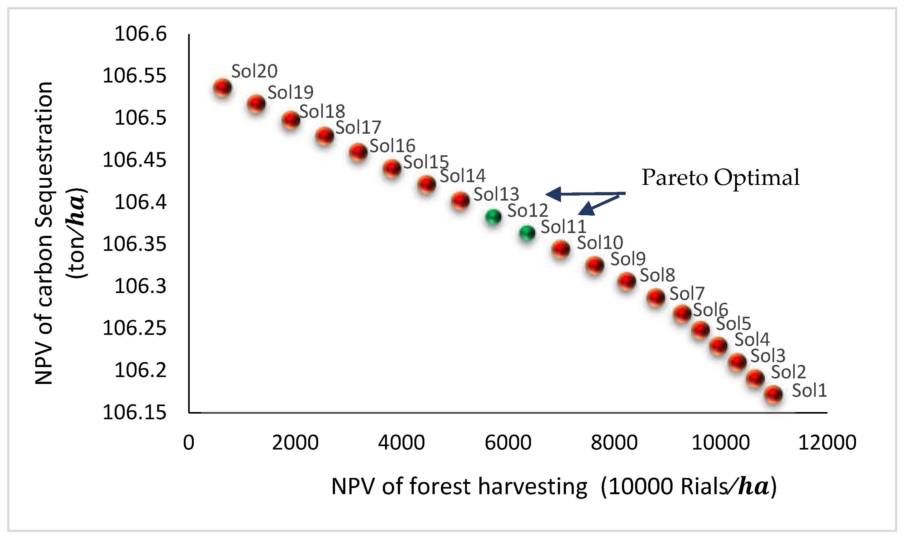
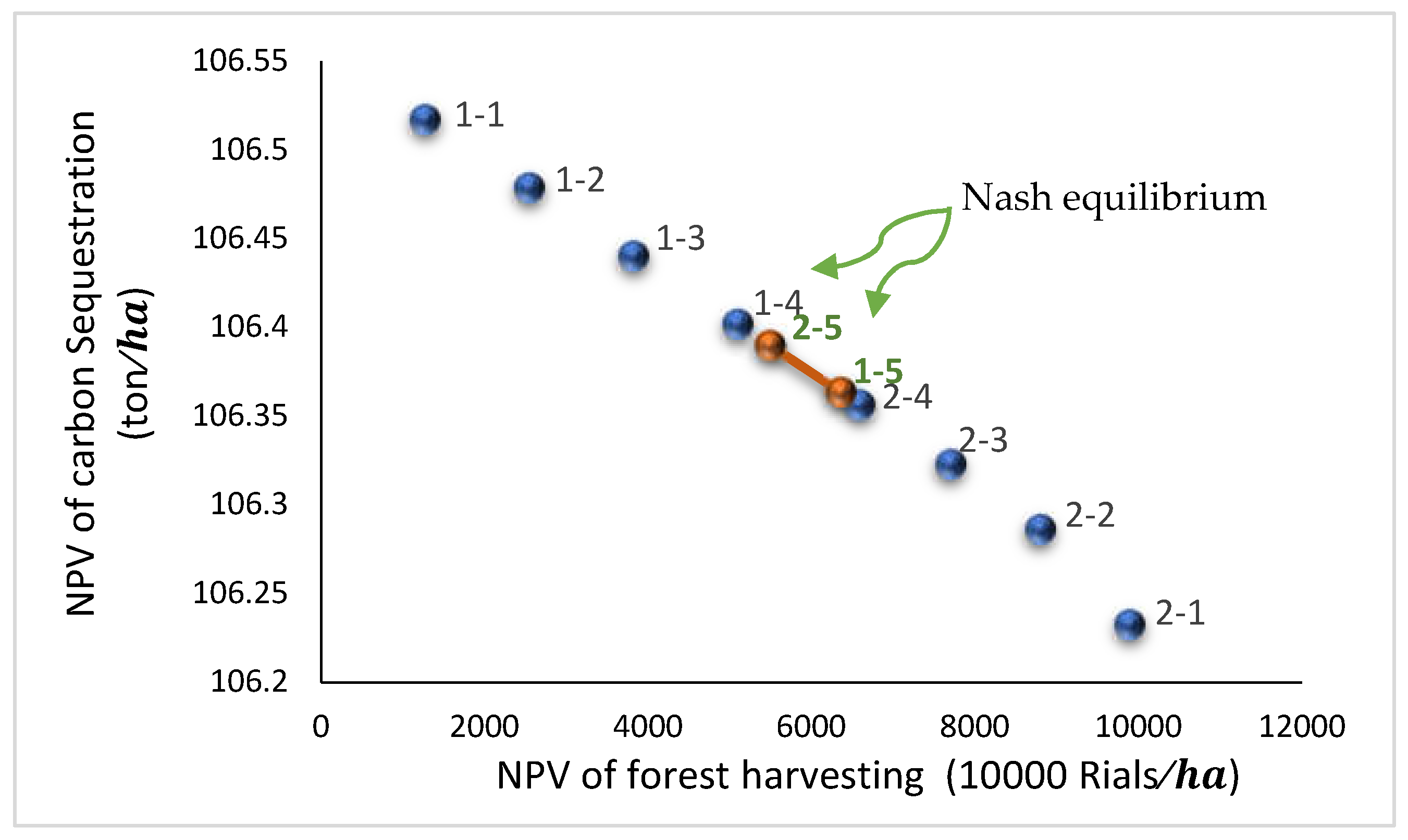
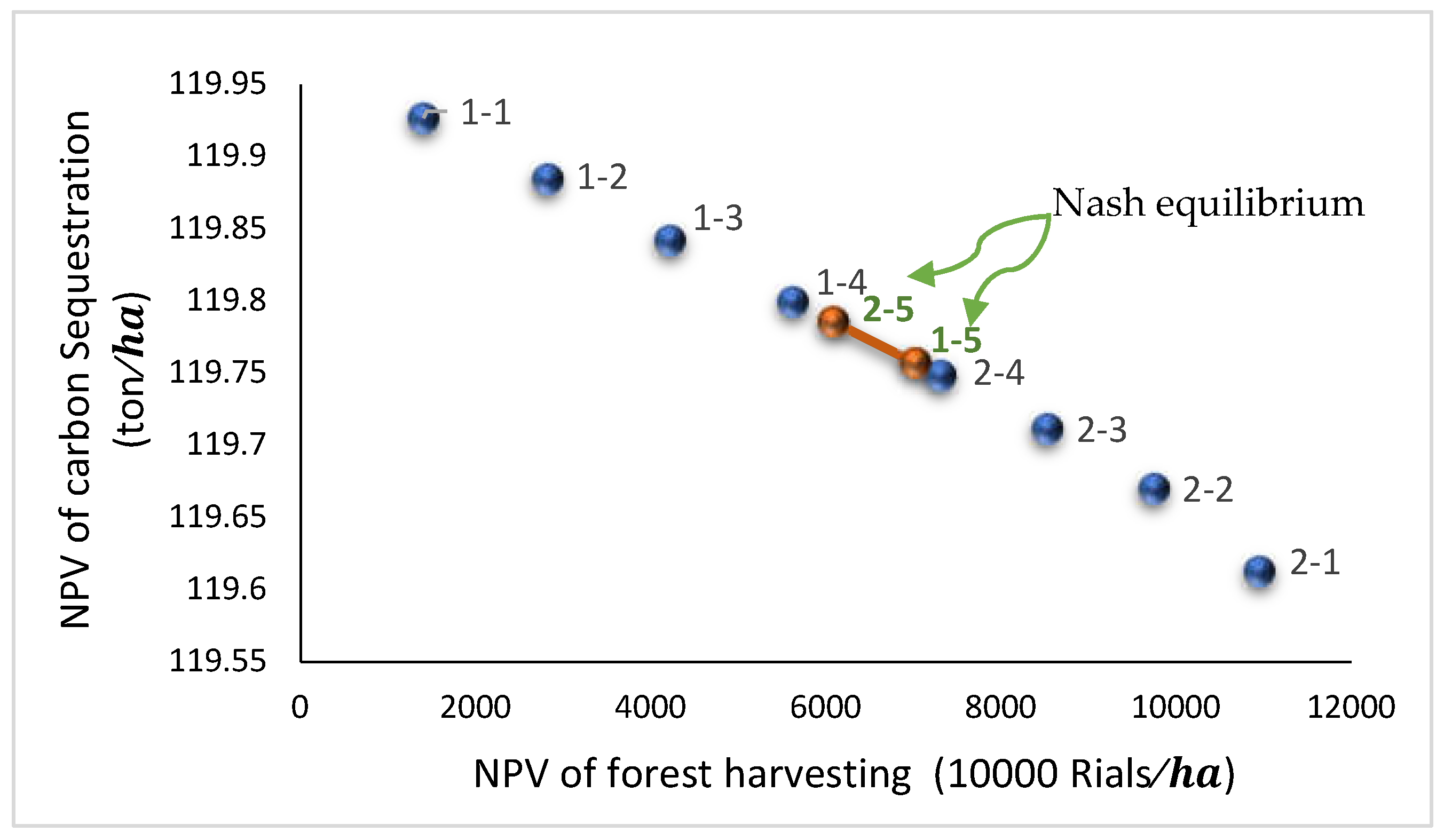
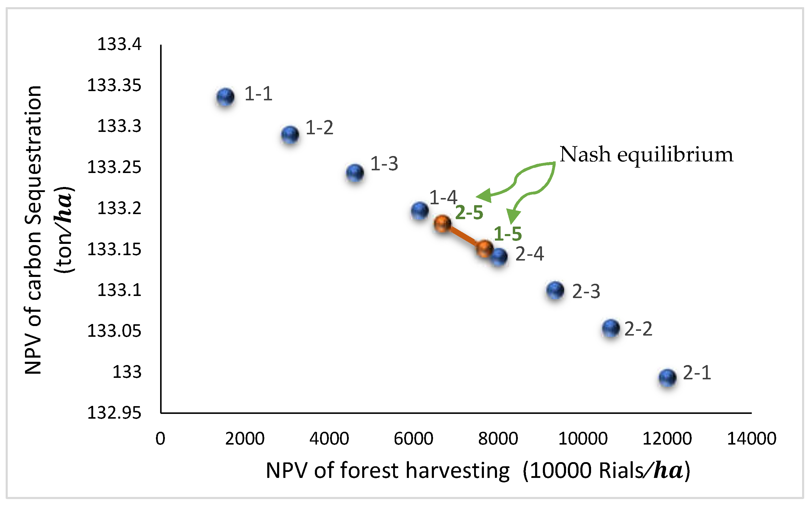
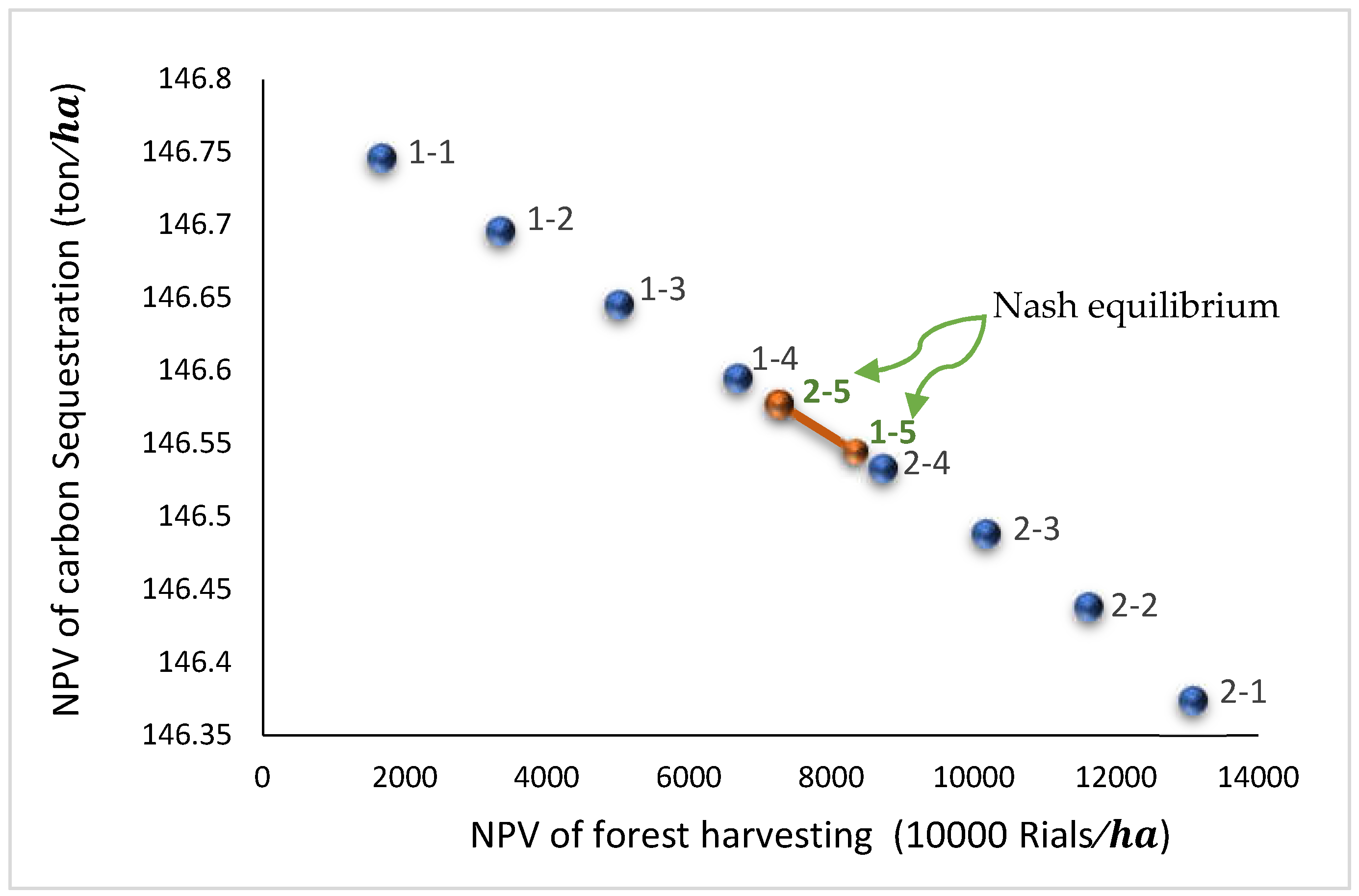
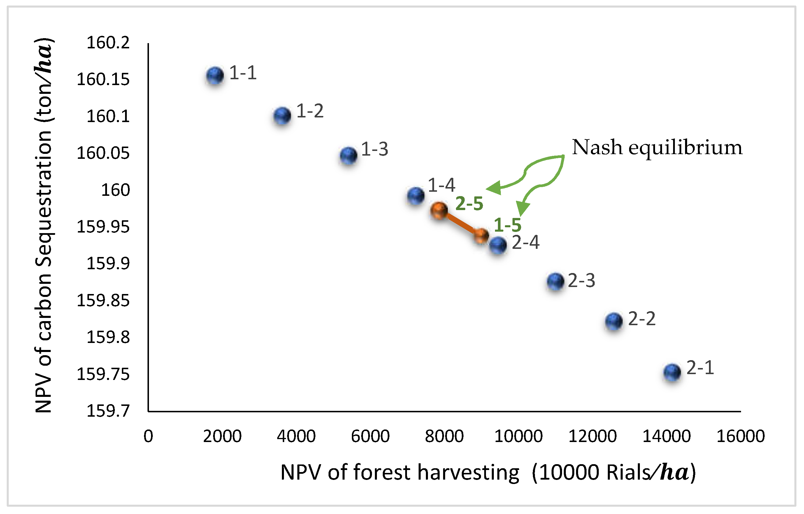
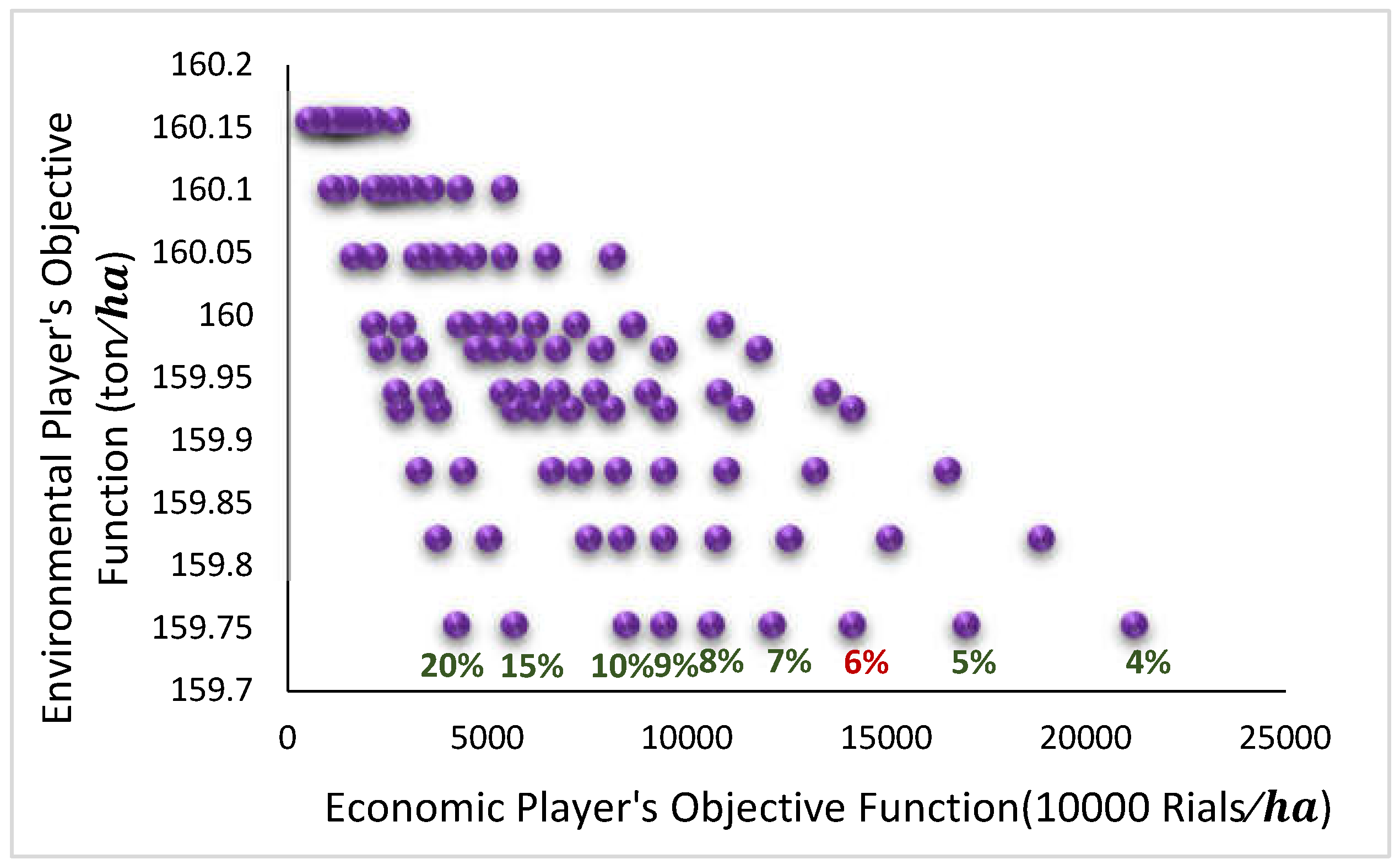
In the fifth round of bargaining, a Nash equilibrium was reached, indicated by the intersection marked "1-5" and "2-5." At this equilibrium point:
The economic player achieved an NPV of 6363.748 (10,000 Rials) and carbon sequestration of 106.3633 (tons/ha).
The environmental player achieved an NPV of 5496.699 (10,000 Rials) and carbon sequestration of 106.3897 tons/ha.

This equilibrium demonstrates a balanced outcome where neither player can improve their position without negatively impacting the other. The positions of the points on the graph reflect the trade-offs each player had to make to reach this balanced state.

Table 14) and Figure 8) show the objective function values for the economic and environmental players for a standing stock of 342.21 (m³/ha). In the fifth round of negotiations, a Nash equilibrium between the two players is reached. The NPV and carbon sequestration at this point for the economic player are 70,232.82 (10,000 Rial/ha) and 119.7571 (t/ha), and for the environmental player are 60,878.36 (10,000 Rial/ha) and 119.7855 (t/ha).

Table 15) and Figure 9) show the objective function values for the economic and environmental players for the stock level of (2), which is 380.48 (m³/ha). In the fifth round of negotiations, a Nash equilibrium was established between the two players. At this equilibrium point, the net present value (NPV) and carbon sequestration for the economic player are 7682.816 (10,000 Rials/ha) and 133.1508 (tons/ha), respectively. For the environmental player, the NPV and carbon sequestration are 6678.973 (10,000 Rials/ha) and 133.1814 (tons/ha), respectively.

Table 16) and Figure 10) display the objective function values for the two players, economic and environmental, with a standing inventory of 418.74 (m³/ha). In the fifth round of bargaining, a Nash equilibrium has been reached between them. At this equilibrium point, the economic player achieves an NPV of 8,342.35 (10,000 Rial/ha) and carbon sequestration of 146.5446 (tons/ha), while the environmental player achieves an NPV of 7,270.11 (10,000 Rial/ha) and carbon sequestration of 146.5772 (tons/ha).

Table 17) and Figure 11) present the objective function values for the economic and environmental players with a standing inventory of 457 (m³/ha). In the fifth round of bargaining, a Nash equilibrium has been achieved between the two players. At this equilibrium point, the NPV and carbon sequestration for each player are as follows: for the economic player, NPV of 9,001.884 (10,000 Rial/ha) and carbon sequestration of 159.9383 (tons/ha); for the environmental player, NPV of 7,861.248 (10,000 Rial/ha) and carbon sequestration of 159.9731 (tons/ha).

Table 18) shows the growth and equilibrium harvest rates at each stock level as well as the stock for each tree species.

Table 19) shows the growth and equilibrium harvest rates for each species at different levels of stock for each player.

Table 19) shows the growth and equilibrium harvest rates at each stock level as well as the stock for each tree species.

3.8. Sensitivity Analysis

3.8.1. Multi-Objective Model

The sensitivity of the objective function was analyzed for the multi-objective model at interest rates of 4%, 5%, 6%, 7%, 8%, 9%, 10%, 15%, and 20%, for the optimal stok of 457 (m³/ha). The results indicated that as the interest rate increases, the expected NPV decreases.

Figure 12. Sensitivity of NPV to interest rate changes for optimal stock of 457 (m³/ha).

The analysis shows a clear trend where the increase in the interest rate results in a decrease in the NPV, reflecting the diminishing returns on future revenues when discounted at higher rates.

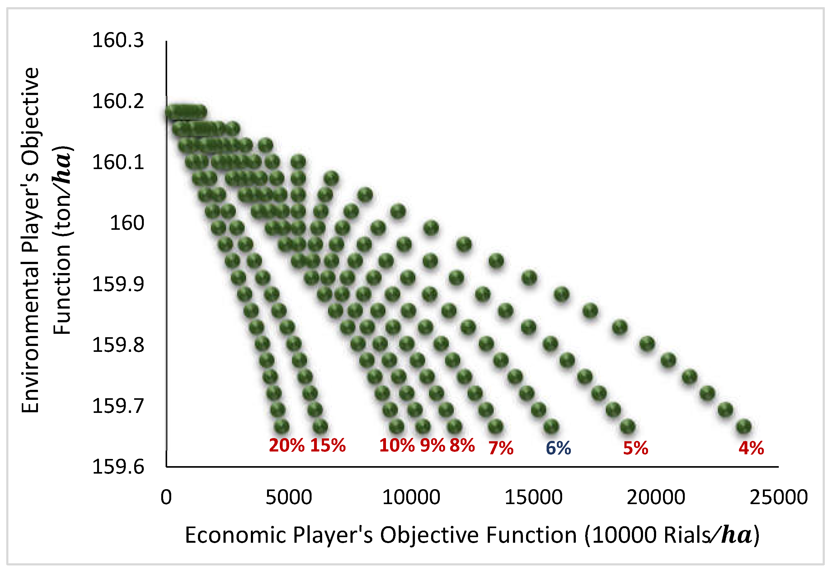
3.8.2. Game Theory Model

The game theory model also examined the variation in the objective function at the same interest rates for the optimal standing stock of 457 m³/ha. Similarly, it was observed that as the interest rate rises, the expected NPV decreases (Figure 13).

For both models, the economic player’s objective function was found to be sensitive to interest rate changes, where the NPV was inversely related to the interest rate. However, changes in the interest rate did not affect the environmental player’s objective function, as the carbon sequestration amount remained constant and unaffected by interest rate variations. While the NPV of carbon sequestration was initially included as a constraint, it was later excluded from both models due to the lack of feasible solutions.

4. Discussion

The Nash equilibrium identified in the game theory model of this study simplifies decision-making conditions for environmental and economic stakeholders, enabling informed choices based on available options. This approach becomes crucial when decision-making is complex due to the involvement of diverse stakeholders, allowing adaptation to environmental challenges while fostering economic growth within the constraints defined by the Nash equilibrium. This study's findings resonate with those of Moradi & Mohammadi Limaei (2018) [73], underscoring the utility of Nash equilibrium in resolving decision-making dilemmas under competitive scenarios. In a similar study, Koltarza (2024) [74] focuses on the use of Nash equilibrium as a tool for developing optimal harvesting strategies. The study demonstrates that employing Nash equilibrium can lead to the development of optimal harvesting strategies that consider both economic and environmental benefits. In another study, Siangulube (2024) [75] emphasizes the necessity of private sector participation and the importance of prioritizing local needs and the demands of marginalized people while downplaying the usefulness of formal laws and regulations as the ultimate means to resolve landscape issues. In similar contexts, Ratner et al. (2022) [76] emphasized that in the absence of trust and other democratic elements, negotiating trade-offs is difficult, and the governance paradigm mostly shifts to relying on dominant formal systems of rules and regulations, which may escalate conflicts.

Comparison between Nash equilibrium values and Pareto optimal values reveals distinct methodologies in game theory and multi-objective optimization. This disparity has been previously discussed by Moradi & Mohammadi Limaei (2018) [73], Madani (2010) [77], and Lee (2012) [57]. The multi-objective optimization model offers a spectrum of Pareto optimal points, each representing a feasible compromise between environmental and economic considerations that decision-makers can select based on stakeholder preferences. In contrast, the game theory model, after iterative negotiation rounds, converges on a Nash equilibrium where players pursue self-interest, presenting decision-makers with a limited yet balanced range of choices encompassing economic and environmental objectives. Eyvindson et al. (2023) [58] emphasizes stakeholder engagement through interactive tools that allow users to examine the impact of different scenarios in forest planning, aiding in better and more balanced decision-making. Their study uses multi-objective optimization techniques to determine Pareto optimal points in forest planning, helping decision-makers find a balance between various objectives.

In this study, direct interaction with stakeholders across different scenarios was not explored. Instead, the focus was on decision-making outcomes using game theory models and multi-objective optimization, specifically aiming for Nash equilibrium and Pareto optimal points in managing the Hyrcanian forests. While the multi-objective model and the Pareto frontier contribute to balancing economic and environmental objectives, Nash equilibrium plays a more prominent role in improving the decision-making process for optimal forest resource management.

Our findings align with Moradi & Mohammadi Limaei's (2018) study [73], which highlights the game theory model's advantage in decision-making by simplifying the selection process. In contrast, the multi-objective epsilon constraint method used here, though effective in ranking and narrowing the Pareto optimal range, provides a broader decision-making scope. Consequently, the game theory model is more efficient for decision-makers seeking to balance environmental protection (EnvP) with economic development (EcoD) goals [73].

Çalışkan and Özden (2022) [78] also emphasize the potential of game theory to enhance sustainability policies in international forestry. They underscore how game theory can illustrate the necessity of strategic cooperation among countries and stakeholders for more effective forest resource management. Their findings indicate that game theory can refine decision-making processes in international forestry policies. Specifically, bargaining games can aid in resource allocation, zero-sum games can assess competitive dynamics between countries, and the prisoner’s dilemma can underscore the importance of strategic cooperation. Our study similarly addresses sustainability in the management of the Hyrcanian forests, aiming to balance economic and environmental objectives through game theory techniques. Both studies explore the impact of varying parameters—such as interest rates in our study and game conditions in Çalışkan and Özden's (2022) [78] study—on outcomes. The parallels between these studies highlight the efficacy of game theory in forest resource management and in enhancing decision-making processes. Both demonstrate that game theory can help achieve a better balance between economic and environmental objectives while fostering stronger cooperation among stakeholders. These shared insights offer a valuable foundation for advancing policies and management strategies in forestry and natural resource management.

Nabhani et al. (2024) [3] investigated the optimization of economic and environmental objectives in ecosystem services under conditions of uncertainty. Their study provides a comprehensive analysis of Pareto optimal points in ecosystem service optimization, demonstrating how these points can represent the balance between various objectives. However, their focus is predominantly on the application of game theory models and multi-objective optimization under deterministic conditions. While the study explores both Pareto optimal points and the distinction between Nash equilibrium and Pareto optimal points, it places greater emphasis on Nash equilibrium. A sensitivity analysis was conducted for both the multi-objective and game theory models at the optimal standing volume level of 457 m³/ha, considering interest rates ranging from 4% to 20%. The results consistently indicate that as interest rates increase, the Net Present Value (NPV) decreases while the harvest volume rises. This trend suggests that higher interest rates incentivize earlier harvesting, as the expected NPV declines with increasing interest rates. These findings are consistent with those of Mohammadi Limaei and Mohammadi (2023) [79].

Çalışkan, H., & Özden, S. (2022) [78] used sensitivity analysis to explore the effects of various game scenarios on decision-making, illustrating how alterations in game conditions can lead to different outcomes. In our study, the sensitivity analysis of interest rates reveals their impact on harvest volume and net present value, demonstrating how fluctuations in interest rates can influence managerial decision-making. This study demonstrates the feasibility of achieving simultaneous economic and environmental objectives through both multi-objective and game theory models in optimizing Hyrcanian forest management. Nabhani et al. (2024) [3] underscore the importance of considering multiple objectives in forest management and policy under uncertain wood prices, preventing undesired effects from a singular or deterministic approach. This work provides insights into trade-offs and synergies, contributing to strategic planning and policy design. Owing to the current logging moratorium on Iran’s Hyrcanian forests, proactive planning is essential for the post-moratorium period. Determining optimal growth and harvest volumes that balance economic benefits with environmental sustainability will be crucial.

5. Conclusions

The modeling framework utilized in this research provides insights into planning sustainable forest harvesting levels o, aiming to maximize forest growth potential while maintaining optimal standing volumes. Furthermore, the model's flexibility allows for the integration of diverse uses such as social benefits and ecotourism, which can be prioritized based on evolving societal needs.

To enhance the resilience and sustainability of forest management practices in the region, integrating climate change considerations into game theory modeling is recommended to prepare for future environmental challenges. Additionally, addressing social concerns alongside economic and environmental goals.

These strategies aim to refine forest management approaches, ensuring alignment with economic, environmental, and social objectives amidst evolving conditions. By adopting these measures, stakeholders can effectively navigate the complexities of forest management and foster sustainable development in the Hyrcanian forests and beyond.

Author Contributions

Data collection and formal analysis, N.A.; Conceptualization, methodology, writing draft, writing review and editing, N.A. and S.M.L.

Funding

This research received no external funding.

Data Availability Statement

The data are available on request from the corresponding author.

Conflicts of Interest

The authors declare no conflict of interest.

References

Pohjanmies, T.; Eyvindson, K.; Triviño, M.; Mönkkönen, M. More is more?: Forest management allocation at different spatial scales to mitigate conflicts between ecosystem services. Landscape Ecology. 2017, 32, 2337–2349. [Google Scholar] [CrossRef]
Mazziotta, A.; Lundström, J.; Forsell, N.; Moor, H.; Eggers, J.; Subramanian, N.; Aquilue, N.; Moran-Ordonez, A.; Brorons, L.; Snall, T. More future synergies and less trade-offs between forest ecosystem services with natural climate solutions instead of bioeconomy solutions. Global Chang Biology. 2022, 28, 6333–6348. [Google Scholar] [CrossRef] [PubMed]
Nabhani, A.; Mardaneh, E.; Sjølie, H.K. Multi-objective optimization of forest ecosystem services under uncertainty. Ecological Modelling. 2024, 494, 110777. [Google Scholar] [CrossRef]
Lohmander, P. Optimization in forestry: Motivation, principles, methods and results. Forest Ecology and Management Seminar Series of SLU, Umea. 2011, December 13.
Marvie Mohajer, M.R. Silvicultur. Press: Tehran University, Iran. 2005, p: 410.
Karami, H.; Rezvani, M.; Jafari, S. Recent Trends in Deforestation and Biodiversity Loss in Iran’s Northern Forests. Journal of Environmental Management. 2023, 315, 112–125. [Google Scholar] [CrossRef]
Jazirehi, M.H. Analysis and assessment of Iranian forestry organization, in Management of Northern Forest and Sustainable Development. Journal of Iranian Natural Resources. 2000, 55, 13–45. [Google Scholar]
Shamekhi, T. Why does the industrial sector coulden›t utilise the ecological potentiel of northern forest. Iranian Journal of Natural Resources. 1993, 46, 79–93. [Google Scholar]
Purnomo, H.; Yasmi, Y.; Prabhu, R.; Hakim, S.; Jafar, A. Collaborative modelling to support forest management: Qualitative systems analysis at Lumut Mountain, Indonesia Small-scale. Forest Economics, Management and Policy. 2003, 2, 259–275. [Google Scholar] [CrossRef]
Linkevičius, E.; Borges, J.G.; Doyle, M.; Pülzl, H.; Nordström, E.M.; Vacik, H.; Brukas, V.; Biber, P.; Teder, M.; Kaimre, P.; Synek, M.; Garcia-Gonzalo, J. Linking forest policy issues and decision support tools in Europe. Forest Policy and Economics. 2019, 103, 4–16. [Google Scholar] [CrossRef]
Nordström, E.M.; Nieuwenhuis, M.; Başkent, E.; Biber, P.; Black, K.; Borges, J.G.; Bugalho, M.; Corradini, G. Forest decision support systems for the analysis of ecosystem services provisioning at the landscape scale under global climate and market change scenarios. European Journal of Forest Research 2019, 138, 561–581. [Google Scholar] [CrossRef]
Eyvindson, K.; Burgas, D.; Antón-Fernández, C.; Hakanen, J.; Emmerich, M.; Klein, J.; Mönkkönen, M.; Snäll, T.; Caicoya, A.T.; Vergarechea, M.; Blattert, C. MultiOptForest: An interactive multi-objective optimization tool for forest planning and scenario analysis. Open Research Europe. 2023, 3. [Google Scholar] [CrossRef]
Raquel, S.; Ferenc, S.; Emery, C., Jr.; Abraham, R. Application of game theory for a groundwater conflict in Mexico. Journal of environmental management. 2007, 84, 560–571. [Google Scholar] [CrossRef] [PubMed]
Lohmander, P. Rational Research in Forest Production and Forest Management with Consideration of Mixed Species Forest Management and Risk. Operations Research for the Future Forest Management, University of Guilan, Iran. 2014, March 8-12.
Soltani, A.; Sankhayan, P.L.; Hofstad, O. Theory of non-cooperative games as a tool to understand state-local conflicts in forest management. Scandinavian Society of Forest Economics Drøbak, Norway. 2016, 46, 208–216. [Google Scholar]
Hartgraves, C.R. The role of planning in multiple use management", in: Proceedings of Multiple-use Management of Forest Resources. Clemson Univ., Clemson, SC. 1979, 191-196.
Bare, B.B.; Briggs, D.G.; Roise, J.P.; and Schreuder, G.F. A survey of systems analysis models in forestry and the forest products industries. European Journal of Operational Research. 1984, 18, 1–18. [Google Scholar] [CrossRef]
Harrison, T.P.; de Kluyver, C.A. MS/OR and the forest products industry: new directions. Interfaces. 1984, 14, 1–7. [Google Scholar] [CrossRef]
Chang, S.J.; Buongiorno, J. A programming model for multiple use forestry. Journal of Environmental Management. 1981, 13, 45–58. [Google Scholar] [CrossRef]
Shaik Md, Y.H.; Robak, E.W. A Forest Management Process to Incorporate Multiple Objectives: a Framework for Systematic Public Input. Forests. 2010, 1, 99–113. [Google Scholar] [CrossRef]
Mohammadi Limaei, S.; Seddigh Koohi, M.; Rostami Shahraji, T. Goal programming approach for sustainable forest management (Case Study; Iranian Caspian Forests). Journal of Forestry Research. 2014, 25, 429–435. [Google Scholar] [CrossRef]
Jafari, A.; Najafi, A.; García Melón, M. Decision-making for the selection of a best wood extraction method: An analytic network process approach. Forest Policy and Economics. 2015, 50, 200–209. [Google Scholar] [CrossRef]
Heaps, T. Convergence of optimal harvesting policies to a normal forest. Journal of Economic Dynamics and Control. 2015, 54, 74–85. [Google Scholar] [CrossRef]
Arias-Rodil, M.; Dieguez-Aranda, U.; Vazquez-Mendez, M.E. A differentiable optimization model for the management of single-species, even-aged stands. Canadian Journal of Forest Research. 2017, 47(4), 506–514. [Google Scholar] [CrossRef]
Gonzalez-Gonzalez, J.M.; Vazquez-Mendez, M.E.; Dieguez-Aranda, U. Simultaneous optimization of even flow and land and timber value in forest planning: a continuous approach. Forest Ecosystem. 2021, 8, 1–14. [Google Scholar] [CrossRef]
Gonzalez-Gonzalez, J.M.; Vazquez-M’endez, M.E.; Dieguez-Aranda, U. Multi-objective models for the forest harvest scheduling problem in a continuous-time framework. Forest Policy and Economics. 2022, 136, 102687. [Google Scholar] [CrossRef]
Blattert, C.; Mönkkönen, M.; Burgas, D.; Di Fulvio, F.; Caicoya, A.T.; Vergarechea, M.; Klein, J.; Hartikainen, M.; Antón-Fernández, C.; Astrup, R.; Emmerich, M.; Forsell, N.; Lukkarinen, J.; Lundström, J.; Pitzén, S.; Poschenrieder, W.; Primmer, E.; Snäll, T.; Eyvindson, E. Climate targets in European timber-producing countries conflict with goals on forest ecosystem services and biodiversity. Communications Earth & Environment 2023, 4. [Google Scholar] [CrossRef]
Eyvindson, K.; Hartikainen, M.; Miettinen, K.; Kangas, A. Integrating risk management tools for regional forest planning: an interactive multiobjective value-at-risk approach. Canadian Journal of Forest Research. 2018, 48, 766–773. [Google Scholar] [CrossRef]
Schroder, S.A.; Tóth, S.F.; Deal, R.L.; Ettl, G.J. Multi-objective optimization to evaluate tradeoffs among forest ecosystem services following fire hazard reduction in the Deschutes National Forest, USA. Ecosystem Services. 2016, 22, 328–347. [Google Scholar] [CrossRef]
Tóth, S.F.; Ettl, G.J.; Könnyű, N.; Rabotyagov, S.S.; Rogers, L.W.; Comnick, J.M. ECOSEL: Multi-objective optimization to sell forest ecosystem services. Forest Policy and Economics. 2013, 35, 73–82. [Google Scholar] [CrossRef]
Tóth, S.F.; McDill, M.E. Finding Efficient Harvest Schedules under Three Conflicting Objectives. Forest Science. 2009, 55, 117–131. [Google Scholar] [CrossRef]
Vergarechea, M.; Astrup, R.; Fischer, C.; Øistad, K.; Blattert, C.; Hartikainen, M.; Eyvindson, K.; Di Fulvio, F.; Forsell, N.; Burgas, D.; Toraño-Caicoya, A.; Mönkkönen, M.; Antón-Fernández, C. Future wood demands and ecosystem services trade-offs: A policy analysis in Norway. Forest Policy and Economics. 2023, 147, 102899. [Google Scholar] [CrossRef]
Mohammadi Limaei, S. Mixed strategy game theory, application in forest industry. Forest Policy and Economics. 2010, 12, 527–531. [Google Scholar] [CrossRef]
Holopainen, M.; Mäkinen, A.; Rasinmäki, J.; Hyytiäinen, K.; Bayazidi, S.; Pietilä, I. Comparison of various sources of uncertainty in stand-level net present value estimates. Forest Policy and Economics. 2010, 12, 377–386. [Google Scholar] [CrossRef]
Alonso-Ayuso, A.; Escudero, L.F.; Guignard, M.; Quinteros, M.; Weintraub, A. Forestry management under uncertainty. Annals of Operations Research. 2011, 190, 17–39. [Google Scholar] [CrossRef]
Piazza, A.; Pagnoncelli, B.K. The optimal harvesting problem under price uncertainty. Annals of Operations Research. 2014, 217, 425–445. [Google Scholar] [CrossRef]
Eyvindson, K.; Kangas, A. Evaluating the required scenario set size for stochastic programming in forest management planning: incorporating inventory and growth model uncertainty. Canadian Journal of Forest Research. 2016, 46. [Google Scholar] [CrossRef]
Alvarez-Miranda, E.; Garcia-Gonzalo, J.; Ulloa-Fierro, F.; Weintraub, A.; Barreiro, S. A multicriteria optimization model for sustainable forest management under climate change uncertainty: An application in Portugal. European Journal of Operational Research. 2018, 269, 79–98. [Google Scholar] [CrossRef]
Pais, C.; Weintraub, A.; Shen, Z.-J.M. Stochastic forestry planning under market and growth uncertainty. Computers & Operations Research. 2023, 153, 106182. [Google Scholar] [CrossRef]
Swindel, B. Theory of games and applications in forestry [Management strategies, mathematical models]. USDA Forest Service, General Technical Report SE (USA). 1984, 26.
Von Neumann, J.; Morgenstern, O. Theory of games and economic behavior; Princeton university press: Princeton, NJ, 1944; p. 625. [Google Scholar]
Nash, J.F. The bargaining problem. Econometrica. 1950, 18, 155–162. [Google Scholar] [CrossRef]
Camerer, C.F. Progress in behavioral game theory. Journal of economic perspectives. 1997, 11, 167–188. [Google Scholar] [CrossRef]
Myerson, R.B. On the Value of Game Theory in Social Science. Rationality and Society. 1992, 4, 62–73. [Google Scholar] [CrossRef]
Zoghi, M.; Safae, A.; Malekmohammadi, B. Insights on Game Theory in Conflict Analysis of land use change (Case Study: Tehran Dar Abad land area). Geographical Urban Planning Research Journal. 2014, 2, 391–407. [Google Scholar]
Davis, J.B. Forest Fire Control Decision Making Under Conditions of Uncertainty. Journal of Forestry. 1968, 66, 626–631. [Google Scholar] [CrossRef]
Pahlavani, P.; Sahraiian, H.R.; Raei, A. Modeling the spreading of forest fire based on a cellular automata using the markov chain and MOLA with a neighborhood filter. Engineering Journal of Geospatial Information Technology. 2017, 5, 99–122. [Google Scholar] [CrossRef]
Carraro, C.; Marchiori, C.; Sgobbi, A. Negotiating on water: insights from non-cooperative bargaining theory. Environment and Development Economics. 2007, 12, 329–349. [Google Scholar] [CrossRef]
Parrachino, I.; Zara, S.; Patrone, F. Cooperative Game Theory and its Application to Natural, Environmental, and Water Resource Issues: 3. Application to Water Resources. World Bank Policy Research Working Paper. 2006, 4074. Available at SSRN: https://ssrn.com/abstract=946833.
Sabuhi, M.; Mojarad, E. Application of Game Theory for Groundwater Resources Management of Atrak. Journal of Agricultural Economics and Development. 2010, 24, 1–12. [Google Scholar]
Homayounfar, M.; Ganji, A.; Khalili, D.; Mousavi, A.A. A Model for Reservoir Operation Based on the Game Theory. Iran-Water Resources Research. 2010, 6, 14–26. [Google Scholar]
Mohammadi Limaei, S. Economically optimal values and decisions in Iranian forest management. Ph.D. Thesis, Swedish University of Agriculture Sciences, Umea, 2006; p. 148. [Google Scholar]
Mohammadi Limaei, S. A game theory approach to the sawnwood and pulpwood markets in the north of Iran. Caspian Journal of Environmental Sciences. 2007, 5, 1–10. [Google Scholar]
Hejazian, M.; Lotfalian, M.; Lindroos, O.; Mohammadi Limaei, S. Wood transportation machine replacement using goal programming. Scandinavian Journal of Forest Research. 2019, 34, 635–642. [Google Scholar] [CrossRef]
Rodrigues, A.; Koeppl, H.; Ohtsuki, H.; Satake, A. A game theoretical model of deforestation in human–environment relationships. Journal of theoretical biology. 2009, 258, 127–134. [Google Scholar] [CrossRef]
Shahi, C.; Shashi, K. An evolutionary game-theoretic approach to the strategies of community members under Joint Forest Management regime. Forest Policy and Economics. 2007, 9, 763–775. [Google Scholar] [CrossRef]
Lee, C.-S. Multi-objective game-theory models for conflict analysis in reservoir watershed management. Chemosphere. 2012, 87, 608–613. [Google Scholar] [CrossRef]
Eyvindson, K.; Burgas, D.; Antón-Fernández, C.; Hakanen, J.; Emmerich, M.; Klein, J.; Mönkkönen, M.; Snäll, T.; Caicoya, A.T.; Vergarechea, M.; Blattert, C. MultiOptForest: An interactive multi-objective optimization tool for forest planning and scenario analysis. Open Research Europe. 2023, 3. [Google Scholar] [CrossRef]
Etemad, S.S.; Mohammadi Limaei, S.; Olsson, L.; Yousefpour, R. Forest management decision-making using goal programming and fuzzy analytic hierarchy process approaches (case study: Hyrcanian forests of Iran). Journal of Forest Science. 2019. 65, 368–379. [CrossRef]
Shafarood Forestry plan booklet. Forestry Planning of District 7 of Shafarood, Watershed Number 9. Guilan Department of Natural Resources and Watershed Management, Rasht, Iran. 2011, 235. (in Persian).
Schaefer, M.B. Some aspects of the dynamics of populations important to the management of the commercial marine fisheries. Inter-American Tropical Tuna Commission Bulletin. 1954, 1, 23–56. [Google Scholar] [CrossRef]
Kabiri Koupaei, K. Carbon sequestration and its spatial pattern in the above-ground woody compartment of a pure and mixed beech stand: A case study of Gorazbon Forest, north of Iran. Ph.D. Thesis, University of Tehran, Karaj, 2009; p. 102. [Google Scholar]
Snowdon, P.; Raison, R.; Keith, H.; Ritson, P.; Grierson, P.; Adams, M.; Montagu, K.; Bi, H.; Burrows, W.; Eamus, D. Protocol for sampling tree and stand biomass. Australian Greenhouse Office. 2002, 31. [Google Scholar] [CrossRef]
Mohammadi Limaei, S.; Lohmander, P. Stochastic dynamic programming with Markov chains for optimal sustainable control of the forest sector with continuous cover forestry Iranian. Journal of Operations Research. 2017, 8, 91–96. [Google Scholar] [CrossRef]
Mohammadi Limaei, S. Economics Optimization of Forest Management. LAP LAMBERT Academic Publication. 2011, p: 140. (February 3, 2011).
Mavrotas, G. Effective implementation of the ε-constraint method in multi-objective mathematical programming problems. Applied mathematics and computation. 2009, 213, 455–465. [Google Scholar] [CrossRef]
Parrachino, I.; Zara, S.; Patrone, F. Cooperative Game Theory and its Application to Natural, Environmental, and Water Resource Issues: 3. Application to Water Resources. World Bank Policy Research Working Paper. 2006, 4074. Available at SSRN: https://ssrn.com/abstract=946833.
Nash, J.F. Noncooperative games. Annals of Mathematics. 1951, 54, 286–295. [Google Scholar] [CrossRef]
Britz, V.; Herings, J.J.; Predtetchinski, A. Theory of the Firm: Bargaining and Competitive Equilibrium. SSRN Electronic Journal 2010, 34. [Google Scholar]
Ücler, G.; Özsahin, S. Money-Physical Capital Nexus: How Valid Is McKinnon Complementarity Hypothesis In Turkish Economy? Alphanumeric Journal. 2015, 2, 1–12. [Google Scholar] [CrossRef]
World Bank. Carbon Pricing Dashboard 2020. Available online: https://carbonpricingdashboard.worldbank.org (accessed on 21 February 2021).
Gold, Coin, and Currency Information Network. Free Market Exchange Rates 2021. Available online: https://www.tgju.org/currency (accessed on 15 January 2021).
Moradi, S.; Mohammadi Limaei, S.M. Multi-objective game theory model and fuzzy programing approach for sustainable watershed management. Land Use Policy. 2018, 71, 363–371. [Google Scholar] [CrossRef]
Koltarza, J. Application of Nash equilibrium for developing an optimal forest harvesting strategy in Toruń Forest District. Computer Science and Game Theory, 2024; 11. [Google Scholar] [CrossRef]
Siangulube, F.S. The Role of Multistakeholder Platforms in Environmental Governance: Analyzing Stakeholder Perceptions in Kalomo District, Zambia, Using Q-Method. Environmental Management. 2024, 74, 13–30. [Google Scholar] [CrossRef]
Ratner, B.D.; Larson, A.M.; Sarmiento Barletti, J.P.; ElDidi, H.; Catacutan, D.; Flintan, F.; Suhardiman, D.; Falk, T.; Meinzen-Dick, R. Multistakeholder platforms for natural resource governance: Lessons from eight landscape-level cases. Ecology and Society. 2022, 27, 2. [Google Scholar] [CrossRef]
Madani, K.; Rouhani, O.M.; Mirchi, A.; Gholizadeh, S. A negotiation support system for resolving an international trans-boundary natural resource conflict. Environmental modelling & software. 2014, 51, 240–249. [Google Scholar] [CrossRef]
Çalışkan, H.; Özden, S. Game Theory Approach to Decision Making Processes in International Forestry Policies. ASEAN Journal of Science and Technology. 2022, 3, 7–13. [Google Scholar]
Mohammadi Limaei, S.; Mohammadi, Z. Optimal Forest Management Using Stochastic Dynamic Programming Approach–A Case Study from the Hyrcanian Forests of Iran. Journal of Sustainable Forestry. 2023, 42, 120–134. [Google Scholar] [CrossRef]

Figure 1. Study Area: a) Guilan Province, b) Shafarood Watershed, c) District (7) Bagahe Zamin.

Figure 2. Pareto Optimal frontier at forest stock level (1).

Figure 3. Pareto Optimal frontier at forest stock level (2).

Figure 4. Pareto Optimal frontier at forest stock level (3).

Figure 5. Pareto Optimal frontier at forest stock level (4).

Figure 6. Pareto Optimal frontier at forest stock level (5).

Figure 7. Range of objective function variations for each player at the stock level of (1).

Figure 8. Range of objective function variations for each player at the stock level of (2).

Figure 9. Range of objective function variations for each player at the stock level of (3).

Figure 10. Range of objective function variations for each player at the stock level of (4).

Figure 11. Range of objective function variations for each player at the stock level of (5).

Figure 13. Sensitivity of NPV to Interest Rate Changes for Optimal Standing Inventory of 457 (m³/ha).

Table 1. Input Parameters of the Bi-Objective Game Theory Model.

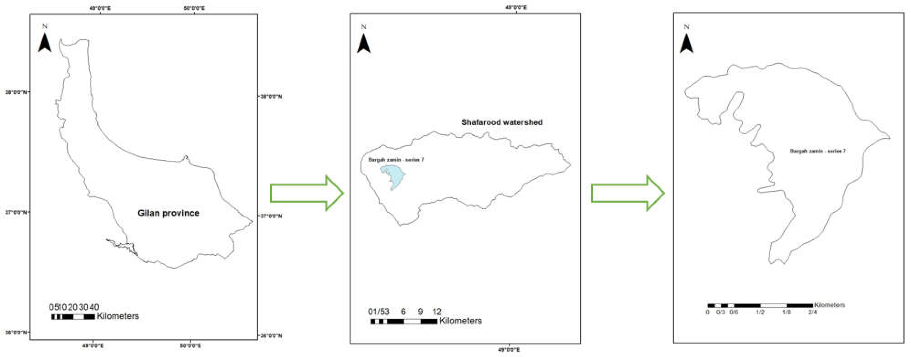
Parameters	Explanations
$\partial_{b}$	The NPV of timber harvesting of species b
$h_{b}$	Amount of harvesting coefficient for species b
${T h}_{b}$	Growth rate of species b
${N H}_{b}$	Number of species b per ha
${V H}_{b}$	Volume of species b per ha
$\tilde{P}$	Maximum number of labour
$π_{b}$	coefficient used for each labour
$\tilde{I P}$	Income of each labour
$d_{p}$	Income coefficient from each labour for harvesting species b
$G_{b}$	Allowed growth capacity for species b
$Q_{b}$	Growth coefficient for species b
${I n v}_{b}$	Optimal inventory for species b
${v h v}_{b}$	Value ofharvestable volume for species b
$f_{b}$	Coefficient of harvestable volume for Species b
$\tilde{i n c o m e}$	Total NPV
$m_{b}$	NPV Coefficient
$\tilde{c s}$	Amount of carbon sequestration
$l_{b}$	Carbon sequestration coefficient

Table 2. Objective functions and input constraints for both models.

(1)	$M a x c = \sum_{b} {\partial_{b} x}_{b}$
(2)	$M a x = \sum_{b} {Q_{b} . x}_{b}$
(3)	${h_{b} . x}_{b} \leq {T h}_{b}$	$\forall b \in B$
(4)	$x_{b} \leq {N H}_{b}$	$\forall b \in B$
(5)	$x_{b} \leq {V H}_{b}$	$\forall b \in B$
(6)	${Q_{b} . x}_{b} \leq G_{b}$	$\forall b \in B$
(7)	$x_{b} \leq {I n v}_{b}$	$\forall b \in B$
(8)	${f_{b} . x}_{b} \leq {v h v}_{b}$	$\forall b \in B$
(9)	${\sum_{b} x_{b} . π}_{b} \leq \tilde{P}$
(10)	${\sum_{b} x_{b} . d}_{b} \leq \tilde{I P}$
(11)	$\sum_{b} x_{b} \leq 457$
(12)	$m_{b} . x_{b} \geq \tilde{i n c o m e}$	$\forall b \in B$
(13)	$l_{b} . x_{b} \geq c s ̃$	$\forall b \in B$
(14)	$x_{b} \geq 0$

Table 3. Volume and type of studied species.

Species Name	Variable	Acceptable volume (%)	Acceptable Volume(m³/ha)
Beech	X₁	55	251.4
Hornbeam	X₂	13	59.4
Oak	X₃	16	73.1
Alder	X₄	9	41.1
Other industrial species	X₅	7	32
Total	X	100	457

Table 5. Logarithmic Functions and Coefficients for Each Species.

Species Name	Variable	Logarithmic Functions	Predicted volume (m³/ha)	Predicted growth (m³/ha)	Coefficients
Beech	X₁	$Y = 0.3094 \ln (x) - 0.3711$	251.4	1.34	0.0053
Hornbeam	X₂	$Y = 0.1393 \ln (x) - 0.1284$	59.4	0.44	0.0074
Oak	X₃	$Y = 0.0962 \ln (x) - 0.0135$	73.1	0.4	0.0055
Alder	X₄	$Y = 0.1042 \ln (x) + 0.2933$	41.1	0.68	0.0165
Other industrial species	X₅	$Y = 0.1144 \ln (x) + 0.1143$	32	0.51	0.0159
Total	X		457	3.37	-

Table 6. NPV of harvestable volume.

Species Name	Variable	Mean expected stumpage price (10000 Rials/ m³)	Harvestable volume (m³/ha)	NPV of harvestable volume (10000 Rials)
Beech	X₁	667.22	0.67	7175.56
Hornbeam	X₂	377.59	0.22	1333.38
Oak	X₃	405.46	0.2	1301.62
Alder	X₄	571.86	0.34	3120.91
Other industrial species	X₅	540.08	0.255	2210.58
Total	X	-	1.685	15142.05

Table 7. Optimal stock values for each species at different levels.

Objective functions	Solution
Objective functions	( $X_{1}$ ) Beech (m³/ha)	Hornbeam ( $X_{2}$ ) (m³/ha)	( $X_{3}$ ) Alder (m³/ha)	( $X_{4}$ ) Oak (m³/ha)	( $X_{5}$ ) Other (m³/ha)	$Total (X)$ (m³/ha)
$M a x Z_{1} (x)$	170	77.42	3.16	37.11	16.26	303.96
$M a x Z_{1} (x)$	190.35	72.92	20.65	38.11	20.2	342.21
$M a x Z_{2} (x)$	210.7	68.41	38.13	39.11	24.13	380.475
	231.05	63.91	55.62	40.1	28.07	418.74
	251.4	59.4	73.1	41.1	32	475

Table 8. Optimal values of the Pareto for objective functions at stock level one.

Grid	Solutions	NPV of forest harvesting (Z₁) (10000 Rials/ha)	NPV of carbon sequestration (Z₂) (ton/ha)	Growth (G) (m³/ha)	Amount of harvest (m³/ha)
Grid 1 (303.96 m³/ha)	Solution 1	10993.4	106.17	1.185	1.128
	Solution 2	10648.08	106.19	1.24	1.073
	Solution 3	10302.76	106.21	1.295	1.018
	Solution 4	9957.43	106.23	1.35	0.963
	Solution 5	9612.11	106.25	1.4	0.913
	Solution 6	9266.79	106.27	1.459	0.854
	Solution 7	8779.62	106.29	1.519	0.794
	Solution 8	8223.06	106.31	1.581	0.732
	Solution 9	7626.5	106.32	1.645	0.668
	Solution 10	6995.12	106.34	1.712	0.601
	Solution 11	6363.75	106.36	1.778	0.535
	Solution 12	5732.37	106.38	1.844	0.469
	Solution 13	5101	106.4	1.91	0.403
	Solution 14	4463.93	106.42	1.969	0.344
	Solution 15	3826.22	106.44	2.026	0.287
	Solution 16	3188.52	106.46	2.083	0.23
	Solution 17	2550.82	106.48	2.141	0.172
	Solution 18	1913.11	106.5	2.198	0.115
	Solution 19	1275.41	106.52	2.255	0.058
	Solution 20	637.7	106.54	2.313	0

Table 9. Pareto Optimal Values for Objective Functions at Level Two.

Grid	Solutions	NPV of forest harvesting (Z₁) (10000 Rials/ha)	NPV of carbon sequestration (Z₂) (ton/ha)	Growth (G) (m³/ha)	Amount of harvest (m³/ha)
Grid 2 (342.21 m³/ha)	Solution 1	12175.67	119.55	1.31	1.25
	Solution 2	11794.61	119.57	1.37	1.19
	Solution 3	11413.54	119.59	1.43	1.13
	Solution 4	11032.47	119.61	1.49	1.07
	Solution 5	10651.41	119.63	1.55	1.01
	Solution 6	10234.36	119.65	1.62	0.94
	Solution 7	9672.23	119.67	1.68	0.88
	Solution 8	9058.06	119.69	1.75	0.81
	Solution 9	8416.74	119.71	1.82	0.74
	Solution 10	7720.01	119.74	1.89	0.67
	Solution 11	7023.28	119.76	1.97	0.59
	Solution 12	6326.55	119.78	2.04	0.52
	Solution 13	5629.71	119.8	2.11	0.45
	Solution 14	4926	119.82	2.18	0.38
	Solution 15	4222.28	119.84	2.24	0.32
	Solution 16	3518.57	119.86	2.3	0.26
	Solution 17	2814.86	119.88	2.37	0.19
	Solution 18	2111.14	119.91	2.43	0.13
	Solution 19	1407.43	119.93	2.49	0.07
	Solution 20	703.14	119.95	2.56	0

Table 10. Pareto Optimal Values for Objective Functions at Level Three.

Grid	Solutions	NPV of forest harvesting (Z₁) (10000 Rials/ha)	NPV of carbon sequestration (Z₂) (ton/ha)	Growth (G) (m³/ha)	Amount of harvest (m³/ha)
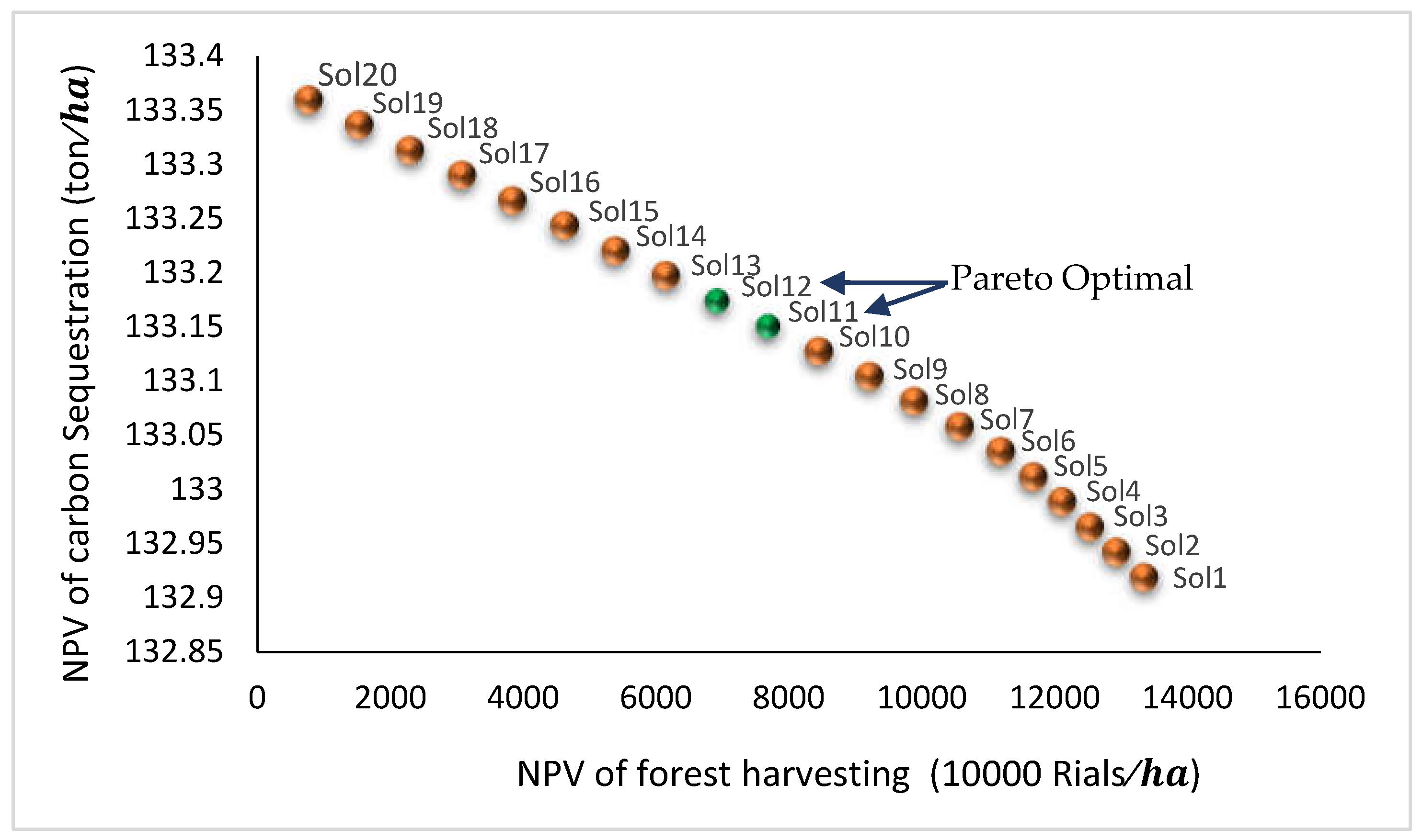
Grid 3 (380.475 m³/ha)	Solution 1	13357.95	132.92	1.44	1.36
	Solution 2	12941.14	132.94	1.5	1.3
	Solution 3	12524.32	132.97	1.57	1.23
	Solution 4	12107.51	132.99	1.63	1.17
	Solution 5	11677.99	133.01	1.7	1.1
	Solution 6	11188.32	133.03	1.77	1.03
	Solution 7	10564.83	133.06	1.85	0.95
	Solution 8	9893.06	133.08	1.92	0.88
	Solution 9	9206.98	133.1	2	0.8
	Solution 10	8444.9	133.13	2.08	0.72
	Solution 11	7682.82	133.15	2.16	0.64
	Solution 12	6920.73	133.17	2.24	0.56
	Solution 13	6157.79	13.2	2.32	0.48
	Solution 14	5388.07	133.22	2.39	0.41
	Solution 15	4618.34	133.24	2.45	0.35
	Solution 16	3848.62	133.27	2.52	0.28
	Solution 17	3078.9	133.29	2.59	0.21
	Solution 18	2309.17	133.31	2.66	0.14
	Solution 19	1539.45	133.34	2.73	0.07
	Solution 20	769.72	133.36	2.8	0

Table 11. Pareto Optimal Values for Objective Functions at Level Four.

Grid	Solutions	NPV of forest harvesting (Z₁) (10000 Rials/ha)	NPV of carbon sequestration (Z₂) (ton/ha)	Growth (G) (m³/ha)	Amount of harvest (m³/ha)
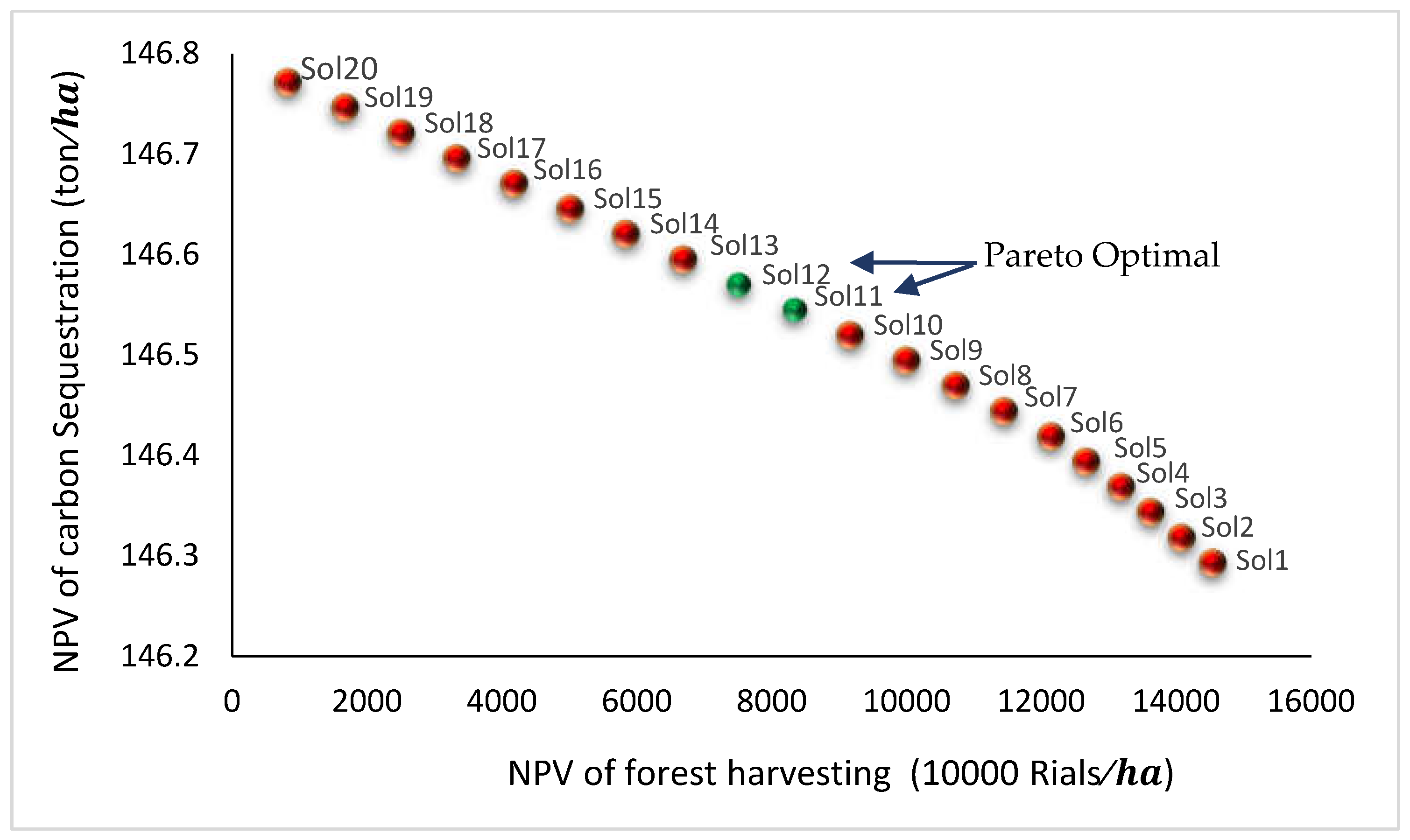
Grid 4 (418.74 m³/ha)	Solution 1	14540.22	146.29	1.56	1.48
	Solution 2	14087.67	146.32	1.63	1.41
	Solution 3	13635.11	146.34	1.7	1.34
	Solution 4	13182.55	146.37	1.78	1.27
	Solution 5	12673.94	146.39	1.85	1.19
	Solution 6	12142.27	146.42	1.93	1.11
	Solution 7	11457.44	146.44	2.01	1.03
	Solution 8	10728.05	146.47	2.09	0.95
	Solution 9	9997.23	146.49	2.17	0.87
	Solution 10	9169.79	146.52	2.26	0.78
	Solution 11	8342.35	146.54	2.35	0.7
	Solution 12	7514.91	146.57	2.43	0.61
	Solution 13	6685.87	146.59	2.52	0.53
	Solution 14	5850.14	146.62	2.59	0.45
	Solution 15	5014.4	146.65	2.67	0.38
	Solution 16	4178.67	146.67	2.74	0.3
	Solution 17	3342.94	146.7	2.82	0.23
	Solution 18	2507.2	146.72	2.89	0.15
	Solution 19	1671.47	146.75	2.97	0.08
	Solution 20	835.73	146.77	3.04	0

Table 12. Pareto Optimal Values for Objective Functions at Level Five.

Grid	Solutions	NPV of forest harvesting (Z₁) (10000 Rials/ha)	NPV of carbon sequestration (Z₂) (ton/ha)	Growth (G) (m³/ha)	Amount of harvest (m³/ha)
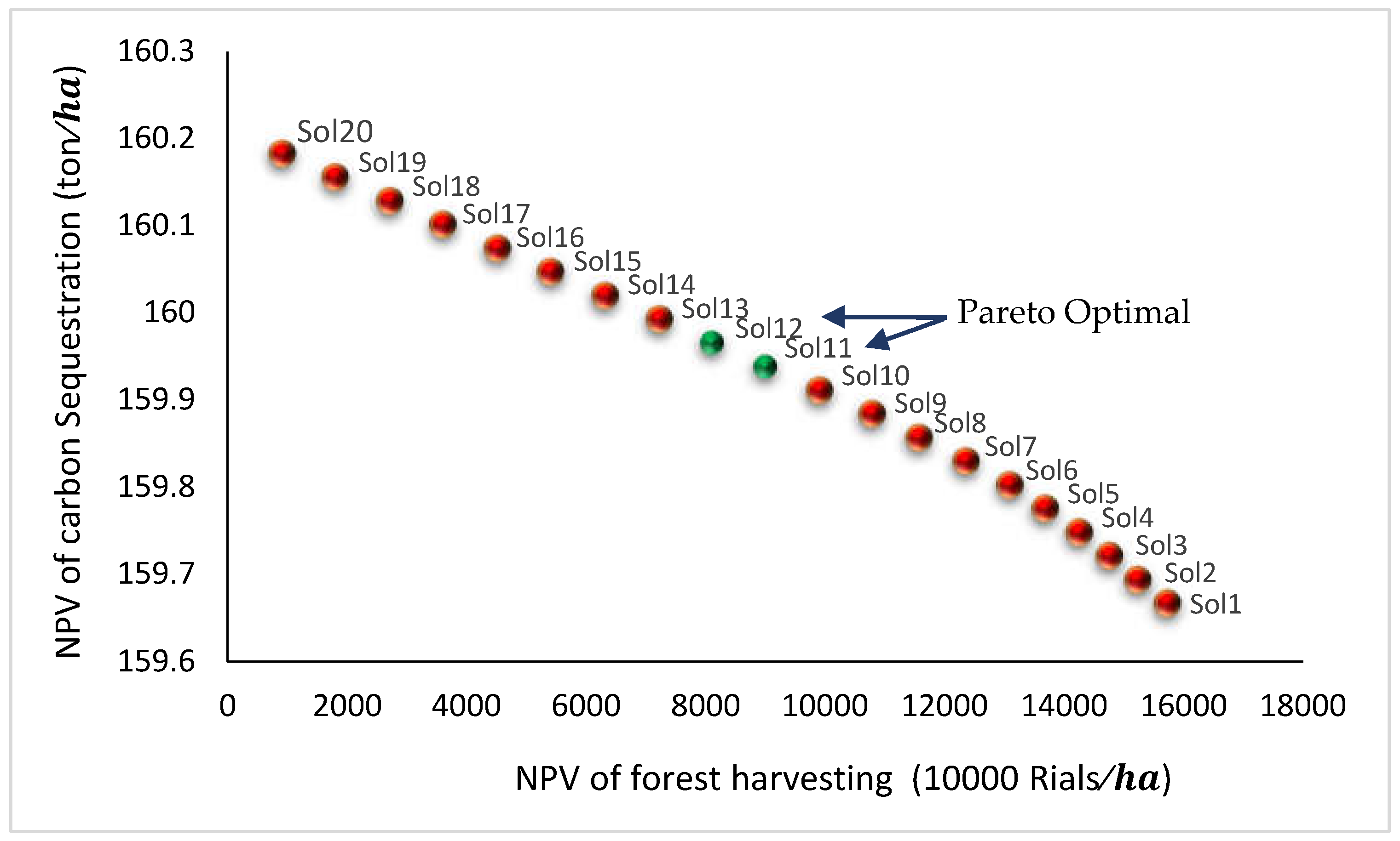
Grid 4 (475 m³/ha)	Solution 1	15722.5	159.67	1.69	1.6
	Solution 2	15234.19	159.69	1.76	1.53
	Solution 3	14745.89	159.72	1.84	1.45
	Solution 4	14243.54	159.75	1.92	1.37
	Solution 5	13669.88	159.78	2	1.29
	Solution 6	13096.23	159.8	2.09	1.2
	Solution 7	12350.05	159.83	2.18	1.11
	Solution 8	11536.05	159.86	2.26	1.03
	Solution 9	10776.06	159.88	2.35	0.94
	Solution 10	9894.68	159.9	2.44	0.85
	Solution 11	9001.88	159.94	2.54	0.75
	Solution 12	8109.09	159.97	2.63	0.66
	Solution 13	7213.95	159.99	2.72	0.57
	Solution 14	6312.21	159.02	2.8	0.49
	Solution 15	5410.46	160.05	2.88	0.41
	Solution 16	4508.72	160.07	2.96	0.32
	Solution 17	3606.98	160.1	3.05	0.24
	Solution 18	2705.23	160.13	3.13	0.16
	Solution 19	1803.49	160.16	3.21	0.08
	Solution 20	901.74	160.18	3.29	0

Table 13. Objective Function Results for Each Player at Level One Standing Stock.

Grid	Game round	Players	NPV of forest harvesting (Z₁) (10000 Rials/ha)	NPV of carbon sequestration (Z₂) (ton/ha)
Gride1 (303.96 m³/ha)	1-1	Player 1	1275.408	106.517
	1-2	Player 2	9894.058	106.2324
	2-1	Player 1	2550.815	106.4786
	2-2	Player 2	8794.718	106.286
	3-1	Player 1	3826.223	106.4402
	3-1	Player 2	7695.378	106.3228
	4-1	Player 1	5101.001	106.4017
	4-2	Player 2	6596.038	106.3562
	5-1	Player 1	6363.748	106.3633
	5-2	Player 2	5496.699	106.3897

Table 14. Objective Function Results for Each Player at Level Two Standing Stock.

Grid	Game round	Players	NPV of forest harvesting (Z₁) (10000 Rials/ha)	NPV of carbon sequestration (Z₂) (ton/ha)
Gride 2 (342.21 m³/ha)	1-1	Player 1	1407.427	119.9267
	1-2	Player 2	10958.1	119.6128
	2-1	Player 1	2814.855	119.8843
	2-2	Player 2	9740.538	119.6699
	3-1	Player 1	4222.282	119.8419
	3-2	Player 2	8522.97	119.7114
	4-1	Player 1	5629.71	119.7995
	4-2	Player 2	7305.403	119.7485
	5-1	Player 1	7023.282	119.7571
	5-2	Player 2	6087.836	119.7855

Table 15. Objective function results for each player at level the stock level of (3).

Grid	Game round	Players	NPV of forest harvesting (Z₁) (10000 Rials/ha)	NPV of carbon sequestration (Z₂) (ton/ha)
Gride3 (380.48 m³/ha)	1-1	Player 1	1539.447	133.3363
	1-2	Player 2	12022.15	132.9933
	2-1	Player 1	3078.895	133.29
	2-2	Player 2	10686.36	133.0539
	3-1	Player 1	4618.342	133.2436
	3-2	Player 2	9350.562	133.1
	4-1	Player 1	6157.79	133.1972
	4-2	Player 2	8014.768	133.1407
	5-1	Player 1	7682.816	133.1508
	5-2	Player 2	6678.973	133.1814

Table 16. Objective function results for each player at the fourth level of stock.

Grid	Game round	Players	NPV of forest harvesting (Z₁) (10000 Rials/ha)	NPV of carbon sequestration (Z₂) (ton/ha)
Gride4 (418.74 m³/ha)	1-1	Player 1	1671.476	146.746
	1-2	Player 2	13086.2	146.3737
	2-1	Player 1	3342.935	146.6975
	2-2	Player 2	11632.18	146.4379
	3-1	Player 1	5014.402	146.6453
	3-2	Player 2	10178.15	146.488
	4-1	Player 1	6685.87	146.5949
	4-2	Player 2	8724.133	146.533
	5-1	Player 1	8342.35	146.5446
	5-2	Player 2	7270.11	146.5772

Table 17. Objective Function Results for Each Player at the fifth level of stock.

Grid	Game round	Players	NPV of forest harvesting (Z₁) (10000 Rials/ha)	NPV of carbon sequestration (Z₂) (ton/ha)
Gride5 (457 m³/ha)	1-1	Player 1	1803.487	160.1557
	1-2	Player 2	14150.25	159.7526
	2-1	Player 1	3606.975	160.1013
	2-2	Player 2	12578	159.8218
	3-1	Player 1	5410.462	160.047
	3-2	Player 2	11005.75	159.8761
	4-1	Player 1	7213.949	159.9927
	4-2	Player 2	9433.497	159.9252
	5-1	Player 1	9001.884	159.9383
	5-2	Player 2	7861.248	159.9731

Table 18. Objective function values, total growth, harvest amount, and stock by species at different levels of stock.

Stock (m³/ha)	Game Round	Objective		Solution
Stock (m³/ha)	Game Round	NPV of carbon sequestration (Z₂) (ton/ha)	NPV of harvesting (Z₂) (10000 Rials/ha)	Growth	Harvest	X₁ (Beech)	X₂ (Hornbea)	X₃ (Alder)	X₄ (Oak)	X₅ (Other)
303.96	5-1	106.36	6363.75	1.78	0.59	170	77.42	3.16	37.11	16.26
303.96	5-2	106.39	5496.7	1.87	0.5
342.21	5-1	119.76	7023.28	1.97	0.65	190.35	72.92	20.65	38.11	20.2
342.21	5-2	119.82	6087.84	2.06	0.56
380.48	5-1	133.15	7682.82	2.16	0.71	210.7	68.41	38.13	39.11	24.13
380.48	5-2	133.18	6678.97	2.26	0.61
418.74	5-1	146.54	8342.35	2.35	0.77	231.05	63.91	55.62	40.1	28.07
418.74	5-2	146.58	7270.11	2.46	0.66
457	5-1	159.94	9001.88	2.54	0.83	251.4	59.4	73.1	41.1	32
457	5-2	159.97	7861.25	2.66	0.71

Table 19. Optimal growth and harvest volumes for each Species at various levels of stock for each player.

Stock (m³/ha)	Harvest/Growth (m³/ha)	Players	Beech	Hornbeam	Alder	Oak	Other
303.96	Growth	Player 1	0.45	0.57	0.017	0.47	0.3
	Growth	Player 2	0.45	0.57	0.017	0.57	0.3
	Harvest	Player 1	0.453	-	-	0.139	-
	Harvest	Player 2	0.453	-	-	0.048	-
342.21	Growth	Player 1	0.51	0.54	0.113	0.49	0.322
	Growth	Player 2	0.51	0.54	0.113	0.58	0.322
	Harvest	Player 1	0.507	-	-	0.145	-
	Harvest	Player 2	0.507	-	-	0.047	-
380.48	Growth	Player 1	0.56	0.51	0.21	0.5	0.38
	Growth	Player 2	0.56	0.51	0.21	0.6	0.38
	Harvest	Player 1	0.562	-	-	0.151	-
	Harvest	Player 2	0.562	-	-	0.046	-
418.74	Growth	Player 1	0.62	0.47	0.3	0.51	0.45
	Growth	Player 2	0.62	0.47	0.3	0.62	0.45
	Harvest	Player 1	0.616	-	-	0.157	-
	Harvest	Player 2	0.616	-	-	0.044	-
457	Growth	Player 1	0.67	0.44	0.4	0.52	0.51
	Growth	Player 2	0.67	0.44	0.4	0.64	0.51
	Harvest	Player 1	0.67	-	-	0.163	-
	Harvest	Player 2	0.67	-	-	0.043	-

Disclaimer/Publisher’s Note: The statements, opinions and data contained in all publications are solely those of the individual author(s) and contributor(s) and not of MDPI and/or the editor(s). MDPI and/or the editor(s) disclaim responsibility for any injury to people or property resulting from any ideas, methods, instructions or products referred to in the content.

© 2024 by the authors. Licensee MDPI, Basel, Switzerland. This article is an open access article distributed under the terms and conditions of the Creative Commons Attribution (CC BY) license (http://creativecommons.org/licenses/by/4.0/).

Copyright: This open access article is published under a Creative Commons CC BY 4.0 license, which permit the free download, distribution, and reuse, provided that the author and preprint are cited in any reuse.

MDPI Initiatives

Important Links

Choose an area of interest and we will send you notifications of new preprints at your preferred frequency.

Disclaimer

Optimal Forest Management Using Multi-Objective and Game Theory Techniques: Considering Environmental and Economic Factors

Abstract

1. Introduction

2. Materials and Methods

2.1. Determination of the Volume per ha Relationship

2.2. Growth Model

2.3. Carbon Sequestration Rate

2.4. Stumpage Price

2.5. Determining the Number of Labour

2.6. Sensitivity Analysis

2.7. Questionnaire Design

2.8. Multi-Objective Model

2.9. ε-epsilon Constraint Method

2.10. Lexicographic Optimization Method

2.11. Multi-Objective Game Theory Model (MOGM)

2.12. Sensitivity Analysis

2.13. Objective Functions and Input Parameters

3. Results

3.1. Determining the Volume per ha for Different Tree Species

3.2. The Amount of Carbon Stored in the Optimal Biomass

3.2.1. The Net Present Value of Carbon Sequestration

3.3. Growth Prediction

3.4. Determining the Relationship for the Number of Labour

3.4.1. Labour Income

3.5. Stumpage Price for Various Tree Species

3.5.1. Net Present Value of Harvestable Volume

3.6. Multi-Objective Model

3.7. Game Theory Model

3.8. Sensitivity Analysis

3.8.1. Multi-Objective Model

3.8.2. Game Theory Model

4. Discussion

5. Conclusions

Author Contributions

Funding

Data Availability Statement

Conflicts of Interest

References

MDPI Initiatives

Important Links

Subscribe