Preprint
Article

Rehabilitated Coal Mine Tailings as Green Cooling Islands in the Metropolitan Ruhr Area (Germany)

Altmetrics

Downloads

77

Views

35

Comments

0

A peer-reviewed article of this preprint also exists.

This version is not peer-reviewed

Submitted:

18 September 2024

Posted:

19 September 2024

You are already at the latest version

Alerts
Abstract
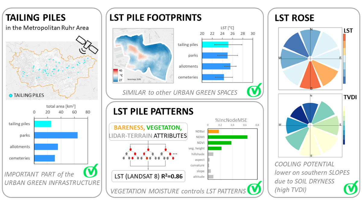
Urban green spaces, such as parks, cemeteries and allotment gardens provide important cooling functions for mitigating the urban heat island (UHI) effect. In the densely populated Ruhr Area (Germany), rehabilitated tailing piles (TP), as relicts of the coal-mining history, are widespread hilly-shaped landscape forms mainly used for local recreation. Their potential role as cooling islands has never been analyzed systematically. Therefore, this study aimed at investigating the TP surface cooling potential in comparison to other urban green spaces (UGS). We analyzed the factors controlling the piles' summer LST pattern using k-mean clustering and Random Forest Regression modeling. Generally, mean LST values of the TPs were comparable to those of other UGSs in the region. Vegetation moisture (NDMI), vitality (NDVI), and height (VH) were found to control the LST pattern of the piles during summer. Soil moisture (TVDI) was directly be related to VH, with highest values on the north and northeast facing slopes and lowest on slopes with south and southeast exposition. Terrain attributes such as altitude, slope, aspect, or curvature were of minor relevance in that context, except on TPs exceeding heights of 125 m. In conclusion, we advise urban planners to maintain and improve the benefit of tailing piles as green cooling islands for UHI mitigation. As one measure, the soil's water-holding capacity could be increased through thicker soil covers or through soil additives during mine tailing rehabilitation, espe-cially on the piles' south and southeast exposition.
Keywords: 
Subject: Environmental and Earth Sciences  -   Remote Sensing

1. Introduction

The urban heat island (UHI) effect is one of the major current and future threats to human health as cities sprawl and densify [1,2,3]. Thus, there is an extensive body of literature on available strategies to reduce the UHI effect and on improving environmental justice in city neighborhoods [4,5,6]. In this context, the cooling effects from urban greening has often been highlighted [7,8,9]. The role of urban green spaces (UGSs) in UHI mitigation has been shown in numerous thermal remote sensing analyses [7,10,11,12,13,14], successfully relating the vegetation abundance reflected by the Normalized Difference Vegetation Index (NDVI) to the land surface temperature (LST). Thus, it is now well accepted that vegetation covers decrease the land surface temperature by up to 3°C compared to the temperature in the surrounding built-up areas, whereby larger UGS areas (>50 ha) showed more substantial cooling effects than smaller green patches [15,16]. In a study by Kuang et al. [17], an LST difference of even over 6°C was found between UGS and built-up areas in some cities.
Generally, the impact of vegetation on the LST is attributed to the fact that plants drastically increase evaporative cooling processes, canopy shading as well as heat adsorption at a local scale [18,19,20]. Nevertheless, more and more research has systemized these impacts and generally differentiate between configuration and composition characteristics controlling the UGS cooling potential [21,22,23]. While configuration comprises of UGS size, shape, complexity, connectivity, and fragmentation, composition defines surface cover and relative abundances of landscape types of the UGS [24,25,26]. While it is still not possible to develop a consensus on specific ways in which varying aspects of UGS configuration interact with land surface temperature (LST) [21], compositional studies clearly showed that areas with a higher percentage of forest vegetation show a greater cooling effect than those dominated by shrub and grass vegetation forms [22,27,28]. Consequently, some studies also focused on tree characteristics such as species, age, or crown diameter and its effect on cooling [14,28]. For example, Rahman et al. [29] observed that fast-growing tree species such as Prunus umineko or P. calleryana generally show a higher stomatal conductivity, providing more cooling. Stumpe et al. (2024) observed that tree age controlled surface cooling, whereas Helletsgruber et al. [30] found that trunk circumference is a valuable indicator for estimating climate-regulating ecosystem services. Similarly, the vertical structure of trees was found to affect their cooling potential [31,32] and He et al. (2024) observed a significant negative correlation between tree canopy height and LST (r = -0.83).
Besides configuration and composition, other factors, such as water availability or terrain attributes, have been discussed in the context of the LST patterns. Concerning water availability, a strong negative correlation has often been found between vegetation moisture reflected by the Normalized Difference Moisture Index (NDMI) and LST pattern across UGS patches, indicating the high relevance of available water for evaporative cooling processes [14,33,34,35]. In this context, the Temperature Vegetation Dryness Index (TVDI) became a well-established parameter for monitoring surface soil moisture [36,37,38,39].
Concerning terrain attributes, several studies characterized the relationship between LST patterns and terrain attributes in natural environments. For example, Tan et al. [34] found a positive correlation between LST and altitude gained from a digital elevation model (DEM) in the Dongting Lake area in China. Karbalaee et al. [40] investigated the relationship between the terrain parameter and LST and observed that an increase in altitude, aspect, and slope leads to a significant decrease in LST. Also, Bai et al. [41] found a relationship between the spatial LST pattern in the Siming Mountain in China and common terrain attributes, although three-dimensional characteristics of the green space showed a higher relevance in that context. Nevertheless, in urban environments, the role of terrain characteristics in the cooling effect of greenspace patterns has generally been neglected.
The majority of these investigations focused on UGSs such as urban parks, urban forests, or urban gardens, with parks being most relevant as urban cooling islands. Consequently, the term “park cooling island (PCI)” arose [18,42,43]. More recent studies also focused on other UGS, such as peri-urban greens or cemeteries [14,44]. However, in the Ruhr Metropolitan Area (Germany), one of the biggest urban agglomerations in Germany, numerous tailing piles from the former coal-mining industry characterize the landscape. The tailing piles are man-made hills often located in residential areas systematically revegetated for local recreation several decades ago. Unlike typical park cooling islands, piles form sloped green areas with high relief energieswhich can thus provide additional cooling effects through drainage of cool air into adjacent residential areas during night time [45]. Although such green tailing piles can potentially play an important role in neighborhood cooling, these green spaces have not been previously considered in the context of UHI mitigation strategies.
Therefore, this study aims at systematically characterizing and understanding the surface cooling of the tailing piles in this region in order to assess their potential as cooling islands. In detail, the objectives of this research were:
(I)
Characterization of the summertime LST footprints of the piles compared to other common UGSs in the Ruhr Metropolitan Region.
(II)
Understanding mean summertime LST values of the piles in the context of vegetation and terrain attributes using the k-mean classification procedure.
(III)
Understanding pixel-based summertime LST values of the piles in the context of vegetation, soil and terrain attributes using random forest regression modeling.

2. Materials and Methods

2.1. Study Area

We focused on the Ruhr Metropolitan Region in North Rhine-Westphalia (Germany) since it is the largest urban economic zone in Germany with about 5.5 million inhabitants and a total area of about 4,400 km2 [46,47].
The area covers the old-industrialized Ruhr area, one of Europe's most important coal fields, where millions of tons of coal were extracted through deep mining in the past century. As a by-product of these activities, large amounts of mine tailings were produced during shaft drilling and coal washing , consisting of sandstone, shale or slate rocks [48]. Most of the mining waste material was dumped in tailing piles, with only smaller amounts being used as underground stowing materials. In the early 1980`s, the regional mining company (Ruhrkohle AG) developed a tailing pile rehabilitation concept, which was integrated into the regional development plan. In this concept, the tailing piles were designed to blend optimally into the surrounding landscape, assuring the protection and restoration of ecological functions [48].
Before establishing a vegetation cover, tailing piles were generally covered with shallow soils (up to 10 cm) and, if necessary, deep soils (up to 1.8 m) for improving water retention and nutrient availability. In 1985, the greening concept [49] was implemented, where shrub and three species were selected and planted depending on soil cover characteristics. In most cases, the pile boundary areas were planted with blackthorn (Prunus spinosa), buckthorn (Hippophae rhamnoides), willow (Salix sp.), and common maple (Acer pseudoplatanus). The main areas were vegetated with red oak (Quercus rubra), wild-growing fruits, birch (Betula sp.), rowanberry (Sorbus aucuparia), and horse chestnut (Aesculus hippocastanum).
Within this study, we focused on tailing piles and their surface cooling potential, but also analyzed the thermal footprints of more common UGSs (parks, allotments, and cemeteries) as a reference. To delineate parks (P), allotments (A), or cemeteries (C) from their surroundings, we used the ‘Authorative Topographic-Cartographic Information System’ (ATKIS). It is the official German nationwide open source digital database for topographic spatial data, updated annually [50]. However, since within the ATKIS database, tailing piles (TP) are not assigned to one ATKIS object group, we used a digital map provided by Heiko Geyer of the Ruhr Regional Association (pers. comm.) for pile delineation.

2.2. Data Acquisition

2.2.1. Land Surface Temperature (LST)

To identify the surface cooling potential of all tailing piles across the Ruhr Area, Landsat 8 scenes for the Ruhr Area were selected for the periods April to September which are available from 2013 to 2023 [51]. The winter months with low sun level (October to March from 2013 to 2023) were also selected, separately. Within these selected timeslots, all relevant Landsat 8 images were filtered concerning a cloud cover of less than 5%, guaranteeing an area-wide pixel coverage. Selected dates of satellite overpassing and the corresponding images are listed and characterized also with respect to the climate conditions during satellite overpassing in Table A1 (Appendix A).
Based on the selected Landsat scenes, the LST and spectral indices were calculated according to the approach of Stumpe et al. [33]. The LST of all selected Landsat 8 OLI/TIRS images was determined based on the spectral band 10 (C2L1 dataset, TIRS 1, 10.6-11.19 μm) using the single band algorithm according to Avdan and Jovanovska [52] and Stathopoulou and Cartalis [53]. The selected Landsat images were also used to calculate spectral indices characterizing vegetation and soil properties as follows.

2.2.2. Vegetation Characteristics (NDVI, NDMI, Height)

The NDVI index was calculated as a proxy for greenness due to its strong correlation with chlorophyll content. It was calculated from the near-infrared Landsat 8 OLI band 5 (0.85-0.88 μm) and the red Landsat 8 OLI band 4 (0.64-0.67 μm) according to [54]. NDVI values range from -1 to 1, with positive values representing vegetated areas and negative values representing non-vegetated areas [54].
The NDMI index is used as proxy for vegetation moisture [55]. This index was calculated from the near-infrared 8 OLI band 5 (0.85-0.88 μm) and the short-wave infrared Landsat 8 OLI band 6 (1.57-1.65 μm). NDMI ranges between -1 and 1, with low values indicating high water stress and high values showing no water stress in the soil-leaf canopy cover level [56].
Vegetation height (VH) was determined based on a normalized digital surface model (nDSM) according to Yu et a. [57]. The corresponding DSM was derived by airborne laser scanning (ALS) with a horizontal and vertical accuracy each of 0.5*0.5 m [50]. For further analysis, the arithmetic means of the VH were calculated for each Landsat grid cell of 30*30 m.

2.2.3. Soil Characteristics (NDBaI, TVDI)

The NDBaI (Normalized Difference Bareness Index) was used in this study since the tailing piles are often characterized by a poorly vegetated and, thus, bare plateau. The index is calculated from the short-wave infrared Landsat 8 OLI band 6 (1.57-1.65 μm) and the thermal infrared Landsat 8 OLI band 10 (10.60-11.19 μm). NDBaI ranges between -1 and 1, where decreasing values indicate an increasing proportion of bare land [58].
The TVDI (Temperature Vegetation Dryness Index) can be used to assess soil moisture. It was determined based on the method proposed by Sandholt et al. [36]. This index is based on the triangular relationship between LST and NDVI values in large areas representing a wide range of surface moisture contents, from wet to dry and from bare soil to fully vegetated surfaces [36]. While the triangle's lower, nearly horizontal wet edge indicates maximal soil wetness and potential evaporation, the dry edge of the triangle represents limiting soil moisture and evaporation. Based on these relationships, the TVDI index was defined by the following equation:
TVDI = (LST - LSTmin) / (LSTmax - LSTmin)
where LST is the observed land surface temperature, and LSTmin and LSTmax are the minimum (wet edge) and maximum (dry edge) functions of NDVI, respectively. For calculation, minimum and maximum LST values of NDVI intervals with a width of 0.01 were extracted across the whole study region and separately for each Landsat summer scene. Then, separately for the extracted minimum and maximum values of the different scenes, these data were linearly fitted, and the corresponding slopes (b and d) and offsets (a and c) were used in the following equation:
LSTmin = (a + b *NDVI)
LSTmax = (c + d *NDVI)
Thus, for each pixel's observed NDVI values, a LSTmin and LSTmax value was calculated and used for TVDI calculation (equation x). TVDI values generally vary between 0 and 1, with a TVDI value of 1 indicating limited soil water content (dry edge), and a TVDI value of 0 (wet edge) indicating sufficient soil water.
To guarantee robust TVDI calculation, regression outliers were eliminated using the Cook`s Distance which summarizes how much a regression model changes when removing the ith observation. Data points from regression processing were excluded if the Cooks`s Distance was higher than 4/n. After outlier correction, we obtained validated regression models with R2 generally higher than 0.96.

2.2.4. Terrain Attributes (Altitude, Slope, Aspect, Curvature)

The altitude (m ASL) of the piles was obtained from digital elevation models (DEMs) derived from airborne laser scanning (ALS) with 1*1 m horizontal resolution and vertical accuracy of 0.01 m from campaigns in 2019 and 2020 [50].
From the DEM, we determined the slope (degree), aspect (radians), and general curvature (degree) as primary terrain attributes using the SAGA Next Gen (Terrain Analysis, Morphometric) implemented in QGIS. Also, hill shading attributes were calculated for each Landsat scene according to the corresponding azimuth and altitude of light [59].
For each terrain variable, the arithmetic means within each Landsat grid cell of 30*30 m were calculated for further statistical analyses. However, since the aspect is a circular variable, the arithmetic means, and statistics that depend on the mean were inappropriate. Thus, we calculated the circular mean ( a ¯ ) as described in the following equation:
a ¯ = arctan 2   ( j = 1 n sin   a j ,   j = 1 n cos   a j )
where the mean direction was found by calculating the arctan2 function of the vector sum of the sinus and cosinus functions, separately. However, arctan2 values are generally varying between 0 and π as well as between 0 and - π , representing, in our case east and west exposition of the tailing piles, respectively. However, since we assumed that according to the azimuth of light north and south expositions of the tailing piles were more important for their LST pattern, the absolute values (ABS) of the circular means were also calculated for Random Forest Regression (RFR) modeling. Values from 0 to π 2 and from π 2   to π then expressed the north and south exposition of the tailing piles, respectively. However, we could no longer distinguish between the east and west expositions.

2.3. Statistical Analysis

To evaluate the importance of independent factors on the LST pattern of the piles, cluster analyses and random forest regression (RFR) were used according to the approach of Stumpe et al. [14]. Thus, we followed the same statistical procedure, as briefly described below.

2.3.1. Cluster Analyses

In the first step, we typified the tailing piles based on their mean LST. According to the different selected Landsat summer scenes, we used each tailing pile's corresponding mean LST values for k-mean classification.
The conventional k-mean algorithm defines k centroids at a rate of one for each cluster so that an object is more similar to objects in its cluster than to objects in a different cluster. The algorithm aims to minimize the sum of square error in the Euclidean distance over all data points [60,61,62]. The optimal number of clusters was identified using the Silhouette method as described in Kodinariya and Makwana [61]. Generally, this method compares within-cluster distances with between-cluster distances, where the greatest difference between clusters indicates the best number of clusters. Analysis was conducted in R version 4.3.3 [63] using the Factoextra package [64].
The average silhouette score and the mean cluster silhouette scores were used to evaluate cluster accuracy. Silhouette scores generally range from -1 to 1, where a threshold is commonly set at 0.5, especially for the average silhouette score. That means scores of more than 0.5 indicate high-quality cluster assignments.
For a final TP typification, the resulting clusters were characterized according to their total tailing pile area, spectral indices, and terrain attributes, which were averaged for each cluster.

2.3.2. Random Forest Regression (RFR)

In the next step, random forest regressions were performed to identify different factors controlling the LST pattern of the tailing piles pixel-wise (30*30 m). We also tested multiple linear regression (MLR), but they failed in prediction accuracy, with R2 being lower than those of the random forest models.
We used the LST distribution of the tailing piles as the dependent variable for RFR modeling, while separate RFR models were run to explain the LST distribution of the different Landsat summer scenes. The separate modeling results were finally averaged. As independent and explaining variables, we used various vegetation (NDVI, NDMI, and VH) and TP terrain characteristics (altitude, slope, curvature, aspect (ABS circular), and hill shading values, while hill shading was calculated separately for each Landsat scenes in dependence of sun angle and azimuth.
The RFR analyses generally belong to the more complex supervised learning algorithms [65,66] and are based on several random decision trees fitted to a dataset with a mean prediction of the ensemble as output. Each tree is grown from a random subset of the features, whereas large numbers of trees run in parallel with no interaction, making the RFR often powerful and accurate [14,66]. However, the number of trees must be optimized to obtain the most stable performance of the RF models. Analysis was conducted in R [63]using the RandomForest package [67].

2.3.3. Feature Importance Analysis

To identify the importance of the independent variables, variables are removed from RFR analyses, assessing how the prediction changes [68]. As indicators, on the one hand, the mean decrease accuracy (%IncMSE) was used, which is a measure of how much the model’s accuracy decreases when a particular variable is randomly permuted. A higher %IncMSE value represents higher variable importance [69]. On the other hand, the mean decrease Gini (IncNodePurity) was used, representing the total decrease in node impurity from splitting on a predictor in the tree construction process averaged over all trees [70]. Both indicators do not differentiate between positive or negative effects on the LST variance. Analysis was conducted in R [63] using the Metrics package [71].

2.3.4. Model Validation

In the first step, each dataset was randomly divided into train (70%) and test (30%) data to describe model performance. In the second step, regression models were fitted using the training datasets so that, in the third step, the dependent variable (LST) was predicted using the trained models and the corresponding test datasets. Finally, the predicted and the observed variables were used to calculate error metrics, such as the coefficient of determination R2, the root mean squared error (RMSE), and the mean absolute error (MAE).

3. Results

3.1. Tailing Pile Characteristics

3.1.1. Spatial Distribution across the Ruhr Area

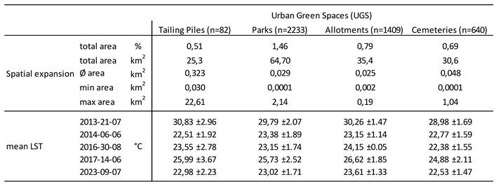
In the first step, tailing piles were characterized by their spatial distribution (Figure 1) and area expansion (Table 1) across the Ruhr Area to assess their role as potential cooling islands within the urban green infrastructure.
The tailing piles are distributed across the main settlements in the Ruhr Area, as indicated by high Normalized Build-up Index (NDBI) values, so they can generally be characterized as urban greens. Nevertheless, larger tailing piles often are found more adjacent to periurban areas indicated by lower NDBI values, while the smaller ones are often surrounded by urban areas represented by high NDBI values.
With 82 tailing piles, their number is much smaller than the more common conventional urban greens such as parks, allotment gardens, or cemeteries (Table 1). Nevertheless, tailing piles comprise large areas with a mean size of 0.323 km2, which is about ten times larger than the mean size of the other UGSs. Consequently, the piles cover 0.51 % of the total Ruhr Area, which is close to the percentages of parks, allotments, and cemeteries, with 1.46, 0.79 and 0.69%, respectively (Table 1).

3.1.2. Morphological Attributes

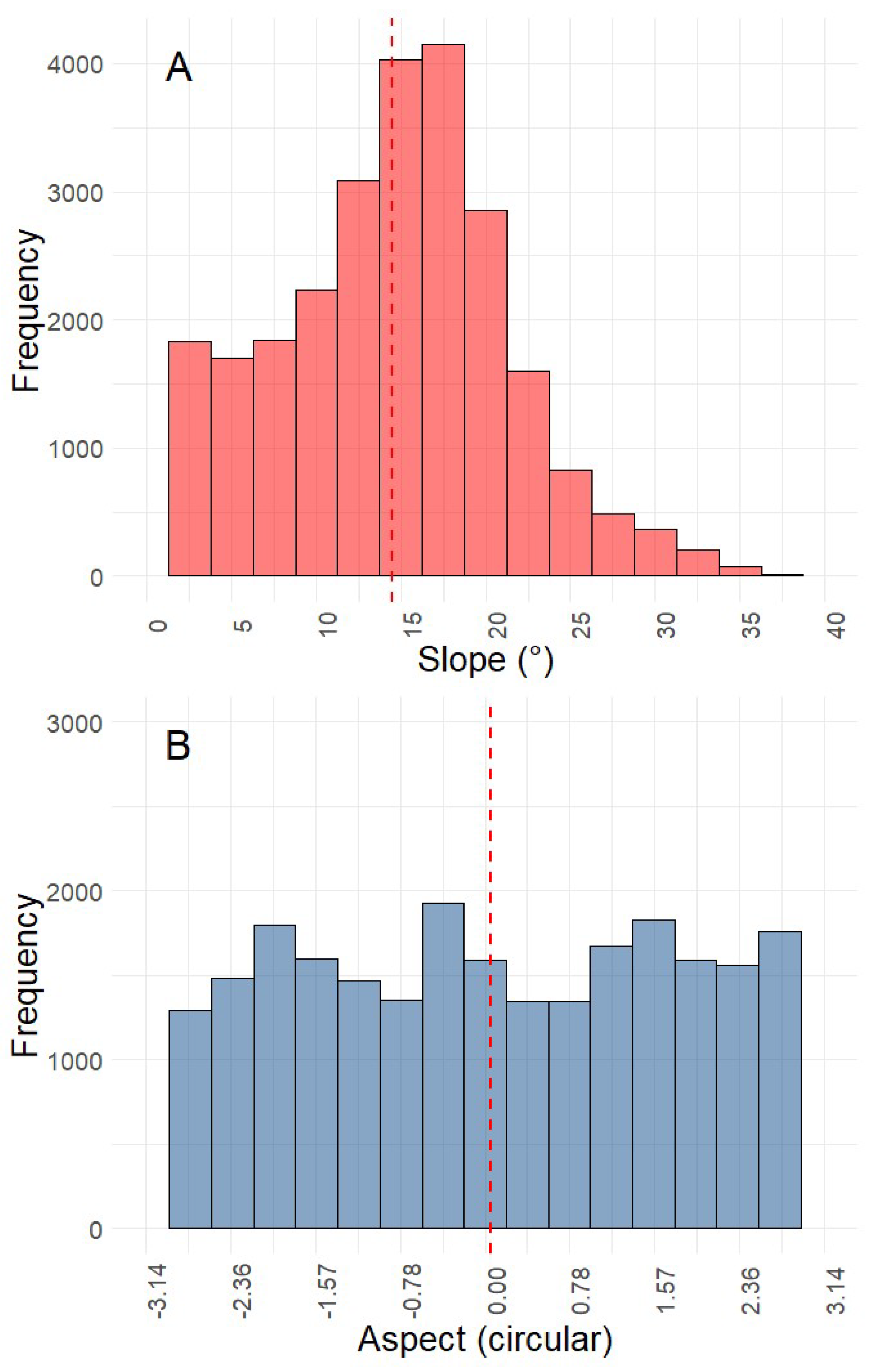
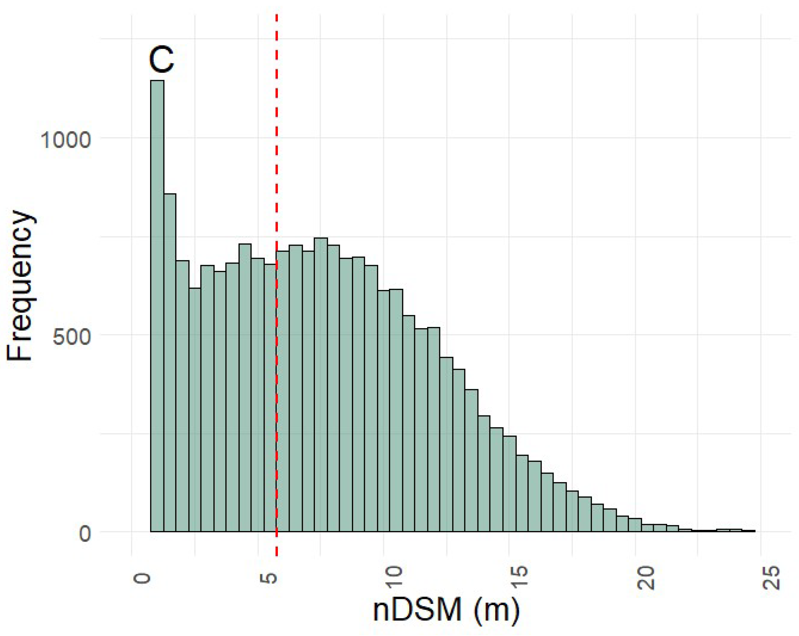
Generally, coal tailing piles are singular hills with elevations reaching 50 to 200 m ASL (Figure 7A) in the rather flat Ruhr area landscape of predominantly 20-60 m ASL. The single hill character is well reflected in the homogenous distribution of the pile aspect values across all directions (Figure 2B). The slope of the pile hillsides varies between 0 and about 40° with a mean of about 14° (Figure 2A). The relatively high frequency of slope values leveling around 0° reflects the hilltop plateaus and the typical step relief stemming from the pile construction. The nDSM histogram in Figure 2C reflects the distribution of plant heights, derived from the aerial laserscan measurements [50]. The predominance of low plant heights (0-0.5 m) shows that large areas of the piles are either free of vegetation or covered by grassland. Often, tailing plateaus are deliberately left bare to illustrate their industrial origin and numerous pathways were constructed for recreational access, also contributing to this nDSM class. The largest part of the piles is covered by shrub and tree vegetation reaching heigths of up to 10 m, with only few areas containing higher trees, reflecting the fact that most piles were only rehabilitated in the last 2-4 decades.

3.1.3. Thermal Footprints

Table 1 summarizes the mean LST values of all tailing piles and the other UGSs for the analysed five different satellite summer scenes. Clearly, the mean LSTs of the piles are similar to those of the other UGSs. Interestingly, the standard deviation of the LST means was generally distinctly higher for the piles than for the other UGS, indicating a higher heterogeneity within this UGS class. The LST differences between the UGS classes could not be tested by ANOVA due to the different LST variances.
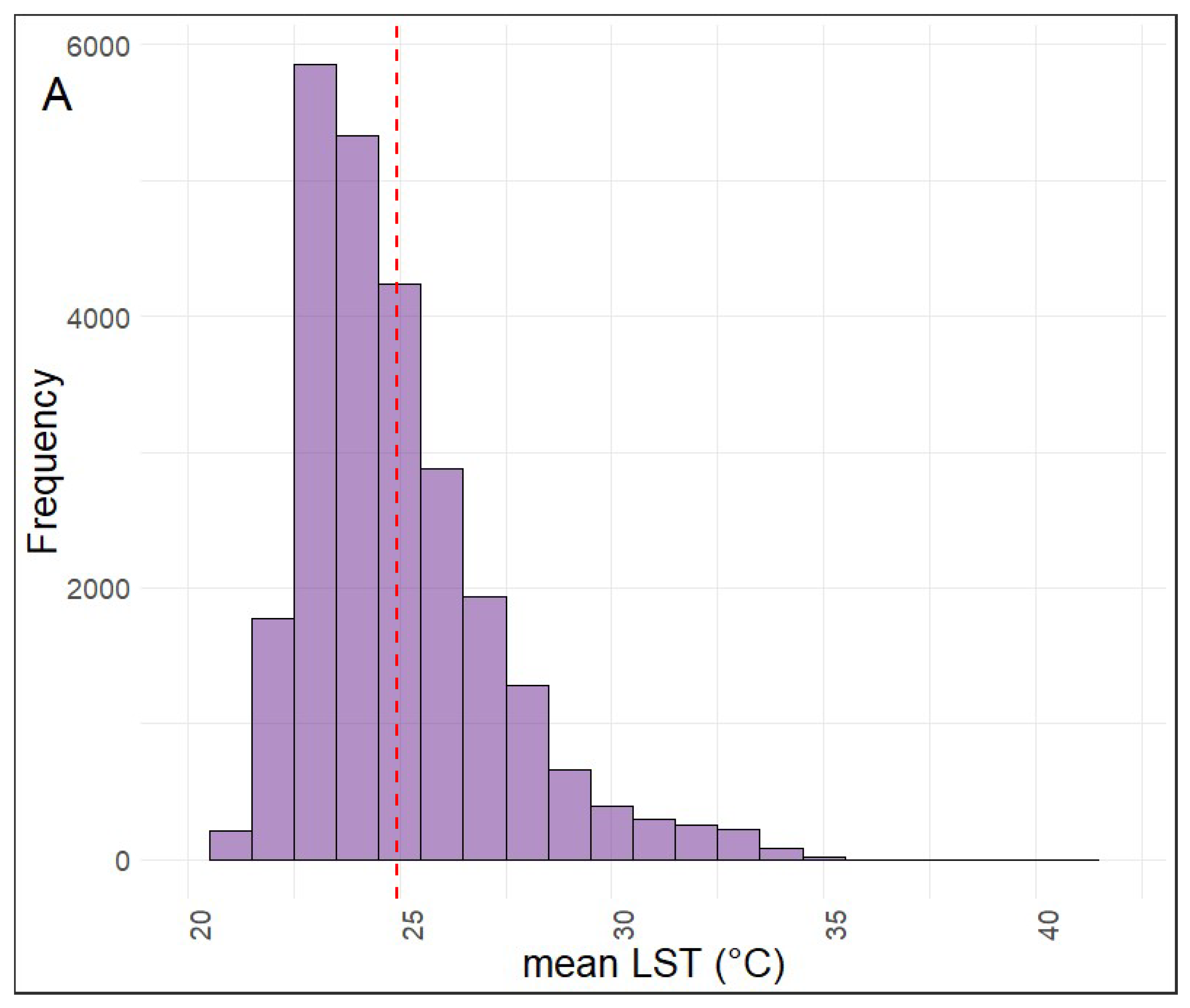
When looking at the frequency distribution of mean summer LSTs on the piles at the pixel level, the histogram shows a pronounced left-skewed normal distribution (Figure 3A). This underlines the very high LST variability among and within the piles. At the same time, the histogram shows that the high LST variance is not only based on a few extreme values but forms a robust distribution of pile surface properties on a small scale. One factor responsible for this may be exposition, since at the time of satellite overpasing around 11 AM, south facing slopes should be more exposed to radiation than north facing slopes. This was confirmed, when the pixels were differentiated according to their position on differently exposed slopes (Figure 3B).
Clearly, south and south-east facing slopes were the warmest and the northern to western slopes were the coolest. However, the LST differences between the slope expositions are not significant and amount to only 1.2°C and thus only partly explain the large LST variability shown in Figure 3A.

3.2. Thermal Typification of Tailing Piles

Based on the mean LST values of the different tailing piles, a cluster analysis was performed, and the analysis included the mean LST values of each satellite summer scene separately. After clustering, we further aimed to characterize warmer or colder pile clusters, considering other properties describing pile vegetation status or topographical parameters for a final pile categorization. Therefore, we hoped to identify different characteristics between the colder and warmer pile classes and be further able to provide recommendations for pile management.
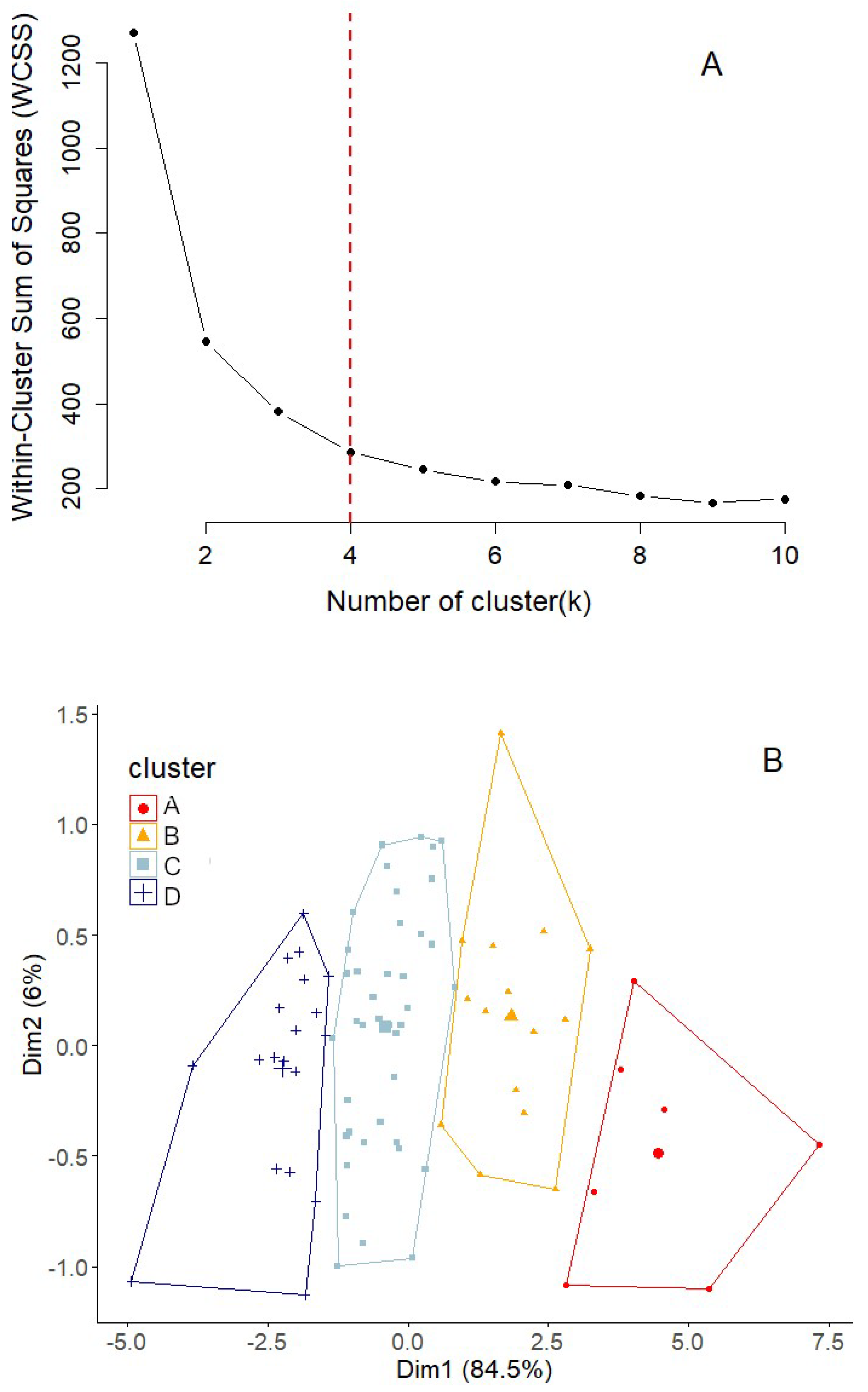
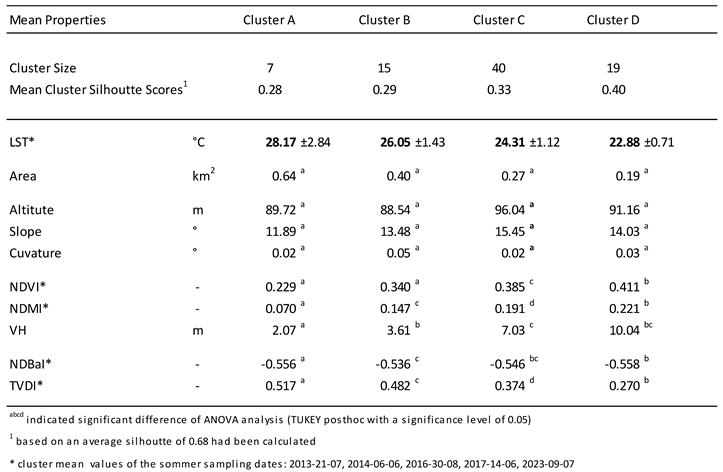
For valid cluster results, we used the within-cluster sum of squares in the first step according to the elbow methods defining the optimal number of four clusters (Figure 4A). Based on this, the k-mean algorithm was used for LST mean clustering. Figure 4 and Table 1 show the cluster assignments and their quality, respectively. Cluster A includes the tailing piles with the highest LST values, which are described by a mean LST of 28.17 °C (Table 2) followed by clusters B, C, and D with a descending order of LST means with 26.05, 24,31, and 22.88°C, respectively. Although the clusters showed a clear separation by mean LSTs, the corresponding standard deviations and mean cluster silhouette scores vary between the clusters, indicating a different quality of cluster assignment. Cluster A contains only seven tailing piles and showed the highest standard deviation and the lowest mean cluster silhouette score of 0.22. Clusters C and D enclose the most tailing piles and thus are more valid clusters with the lowest standard deviation of LST means and the highest mean cluster silhouette scores of 0.33 and 0.40, respectively. Nevertheless, the overall silhouette score of the clustering was calculated at 0.68, indicating a general high-quality cluster assignment that enabled further cluster characterization.
Mean terrain attributes such as the mean tailing pile altitude (DEM) or the mean slope and curvature showed no significant differentiation between the four clusters (ANOVA analyses, p-values>0.05). The mean tailing pile area seems to be related to the cluster LST characteristics since the mean area sizes decline with the mean cluster temperatures, but nevertheless, the mean area sizes between the clusters showed no significant differences (ANOVA analyses, p-values>0.05). However, the spectral indices (NDVI, NDMI) and the VH showed significant differences between the four clusters, with increasing mean index values being related to decreasing mean cluster LSTs. Soil moisture content (TVDI) also differed significantly between the four clusters, indicating more water limitations in the hottest clusters A and B and least in the cool cluster D. With values ranging from -0.558 to -0.536, the soil bareness index (NDBaI) was quite similar among the four clusters, although differences were partly significant. In summary, this shows that vegetation parameters and soil moisture are closely related to the differentiation between the four pile LST types.
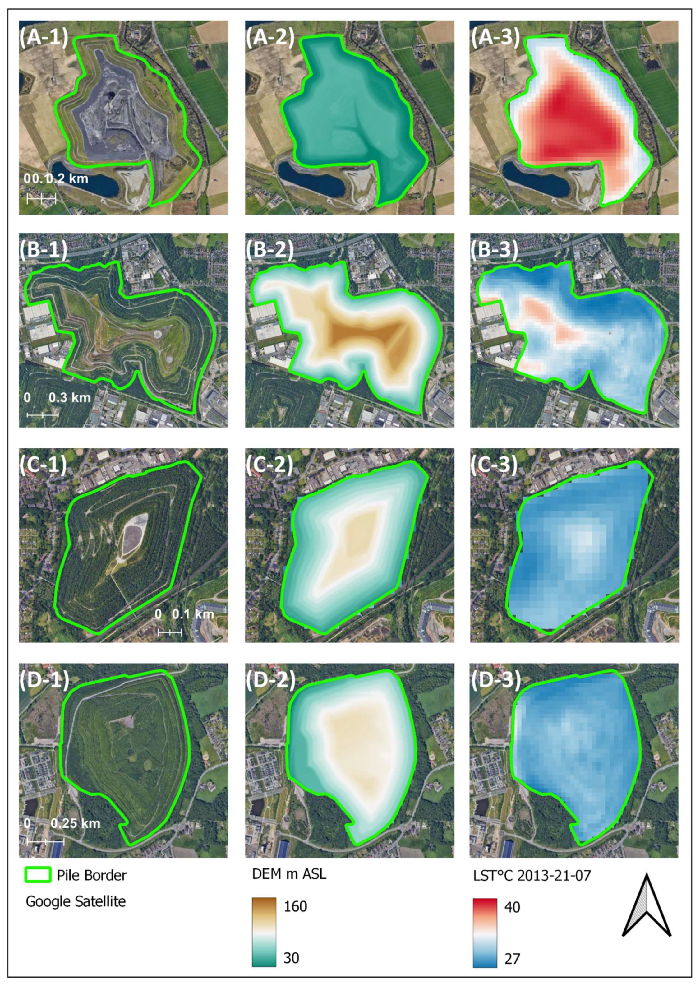
For visualization of these results, Figure 5, shows one arbitrarily selected tailing pile from each cluster as aerial images (A1-D1), DEMs (A2-D2) and as LST patterns (A3-D3). As indicated by the aerial images and the DEMs, the tailing piles generally form hills higher than the surrounding with sloping sides. However, concerning the pile typification, the aerial images also show the distribution of green areas and bare soils. Clearly, the tailing pile “Kohlenhuck” (Figure 5A-1) belonging to the hottest cluster is characterized by a high proportion of bare soil (Figure 5A-3), while the cool piles “Tetraeder” and “Lohberg Nord” (Figure 5C,D) are dominated by tree vegetation.

3.3. Controlling Factors of the LST Distribution of the Tailing Piles
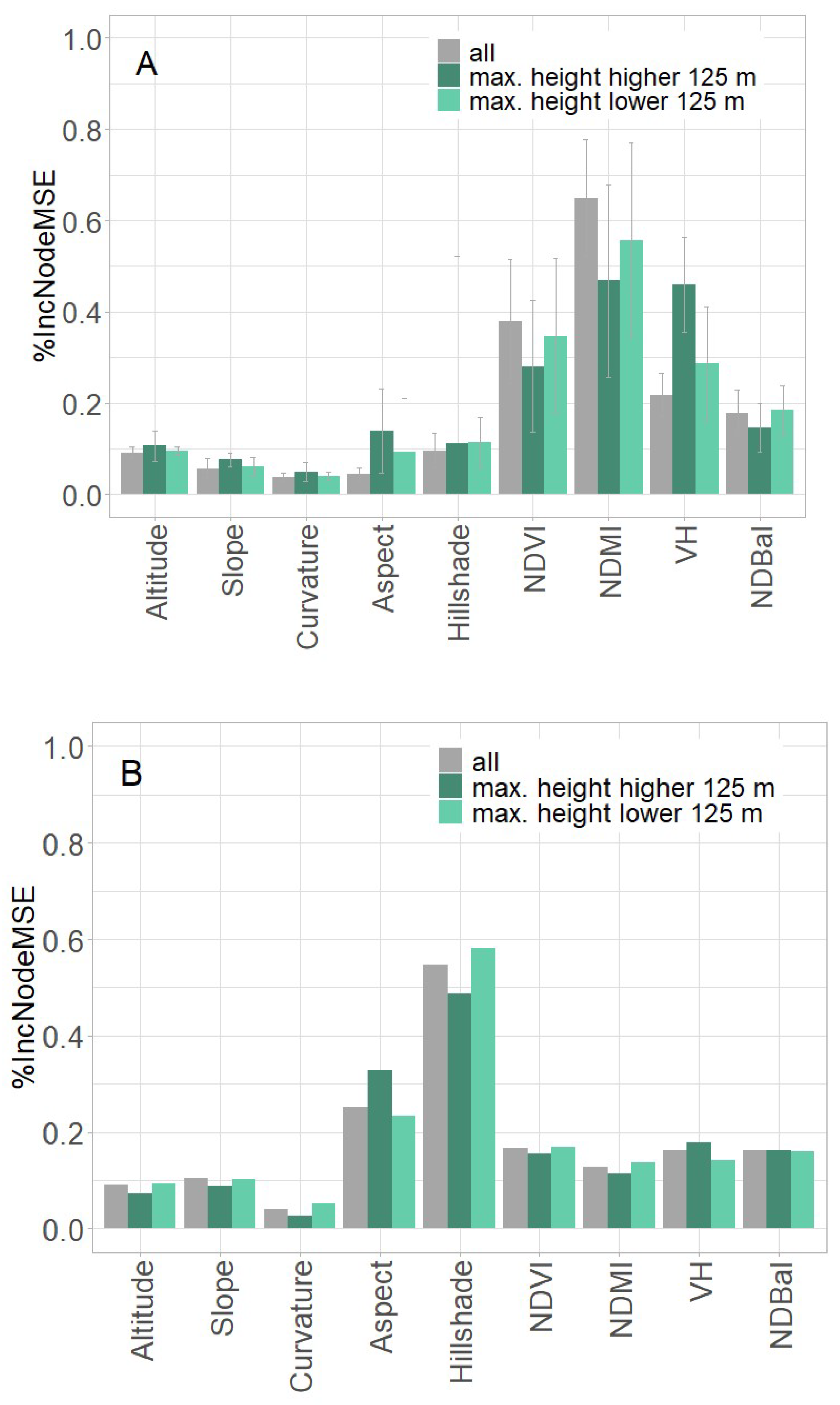
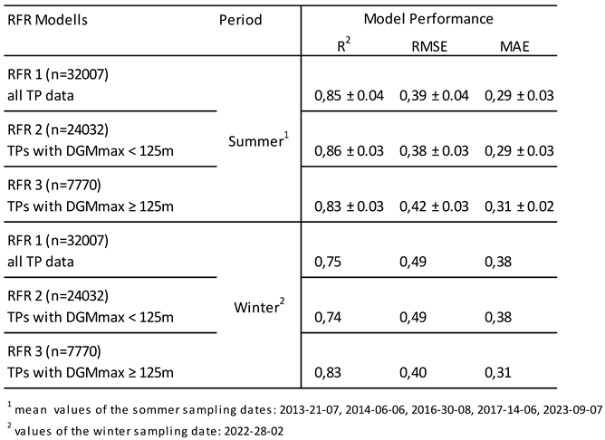
Based on the cluster results, we focused on factors controlling the LST distribution on the tailing piles using a detailed pixel-based analysis. Therefore, in the first step, we run RFR models with the LST as dependent and various independent variables shown in Fig. 6, with models being run separately for the five satellite summer scenes. The model performance was then evaluated based on the mean values from the five models (Table 3). Generally, we obtained high RFR model performances with a mean R2 of 0.85 and a RMSE of 0.39 (Table 3). In order to evaluate the importance of the independent variables across all satellite summer scenes, the %IncNodeMSE values are visualized as mean values in Figure 6A. In accordance with the cluster characterization, the LST variance of the piles was found to be mainly controlled by vegetation properties, which is clearly indicated by high %IncNodeMSE values of the NDVI, the NDMI, and the VH. Although the tailing piles form hilly landscapes, terrain attributes such as pile altitude, slope, curvature, aspect or the hillshade showed relatively low %IncNodeMSE values, thus being less relevant for the LST distribution on the piles. As a control, we also analyzed these dependencies for one Landsat winter scene (Figure 6B), resulting in a less accurate RFR model with a R2 of only 0.75 (Table 3). However, in winter with low sun altitude, the hillshade aspect dominates the LST distribution of the piles, especially the aspect. Due to the dominance of annual herbs and deciduous trees and shrubs, vegetation is inactive in winter and thus is of minor importance for LST variability during this season.
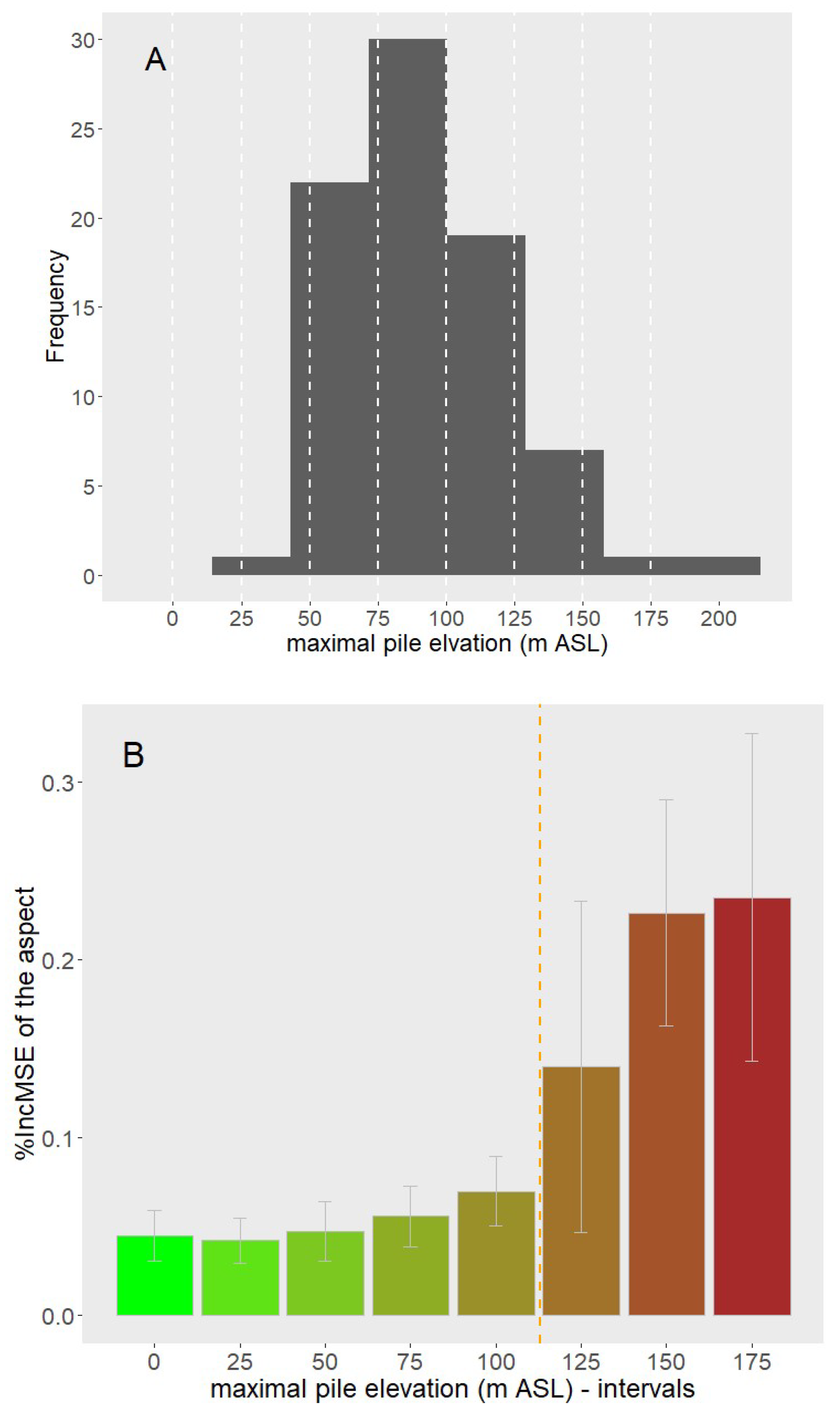
Since shading effects were found to be relevant for the spatial LST pattern in winter, we assumed that they may also matter in summer at certain pile altitudes. Most of the piles reach altitudes up to 125 m, with a maximum frequency between 75 and 100 m ASL (Figure 7A) and only few being higher than 125 m. In order to test for the importance of shading, RFR models for the Landsat summer scenes were run on datasets filtered depending on the maximal pile altitudes in 25 m intervals (Figure 7B). Interestingly, the importance of the aspect, as expressed in the %IncNodeMSE value increased with maximum pile elevation. Due to the decreasing sizes of the datasets, the standard deviation of the %IncNodeMSE values also increases with pile elevation (Figure 7B). Nevertheless, at a maximal pile height of 125 m ASL a threshold was observed where the %IncNodeMSE significantly increased.
Figure 7. Histogram of the tailing pile heights (A) and the variable importance (IncNodeMSE) of the aspect in RFR models differentiated according to pile heights (B). The dotted line indicates the threshold value of the pile height above which a distinct increase of the aspect importance in the RFR models occurs.
Preprints 118563 g007
Consequently, in the next step, the total dataset was divided into two datasets covering piles with maximal pile elevation above and below 125 m ASL. Both datasets were then subjected to the RFR analyses, with the results for both analyses shown in Table 3 and Figure 7. With respect to the Landsat summer scenes, the RFR model performance showed no considerable differences between the three data sets (all pile pixel data, pixel data of piles with DGMmax< 125m ASL or with DGMmax> 125m ASL), but with respect to the Landsat winter scenes model performance improved using pile data with DGMmax > 125m. With an R2 of 0.83, the LST variance of the pixel LST values of piles with DGMmax > 125m was up to 8% better explained by the independent variables than using the unfiltered pile dataset.
Concerning the variable importance, a generally more differentiated pattern of the %IncNodeMSE values across the independent variables was observed using pixel data of piles with DGMmax< 125m ASL and with DGMmax> 125m ASL, separately. For the Landsat summer scenes, the importance of the aspect and the VH increases when pixel data of piles with DGMmax> 125m ASL was used whereas simultaneously, the importance of the NDVI, NDMI, and NDBal decreases. The effects of the dataset separation on the variable importance were similar for the Landsat winter scene but less pronounced.
In summary, it is concluded that a data set separation concerning the maximal pile height resulted in more precise and more differentiated RFR modelling results carving out the importance of the pile aspect and slightly modifying the importance of vegetation properties. Nevertheless, vegetation characteristics were found to be the dominant factors controlling the summer LST pile variability.

3.4. Impact of Soil Moisture on the Pile LST Pattern

Since vegetation characteristics dominate the pile LST pattern, soil moisture as one important controlling factor for transpirational cooling and vegetation health was analyzed using the TVDI index. Since the TVDI calculation is based on the relationship between the LST and the NDVI, this index was excluded as an independent variable in the RFR models. Instead, we analyzed the spatial distribution of the TVDI related to those of the NDMI and VH, assuming that soil moisture is an important indirect factor controlling the LST pattern of the piles.
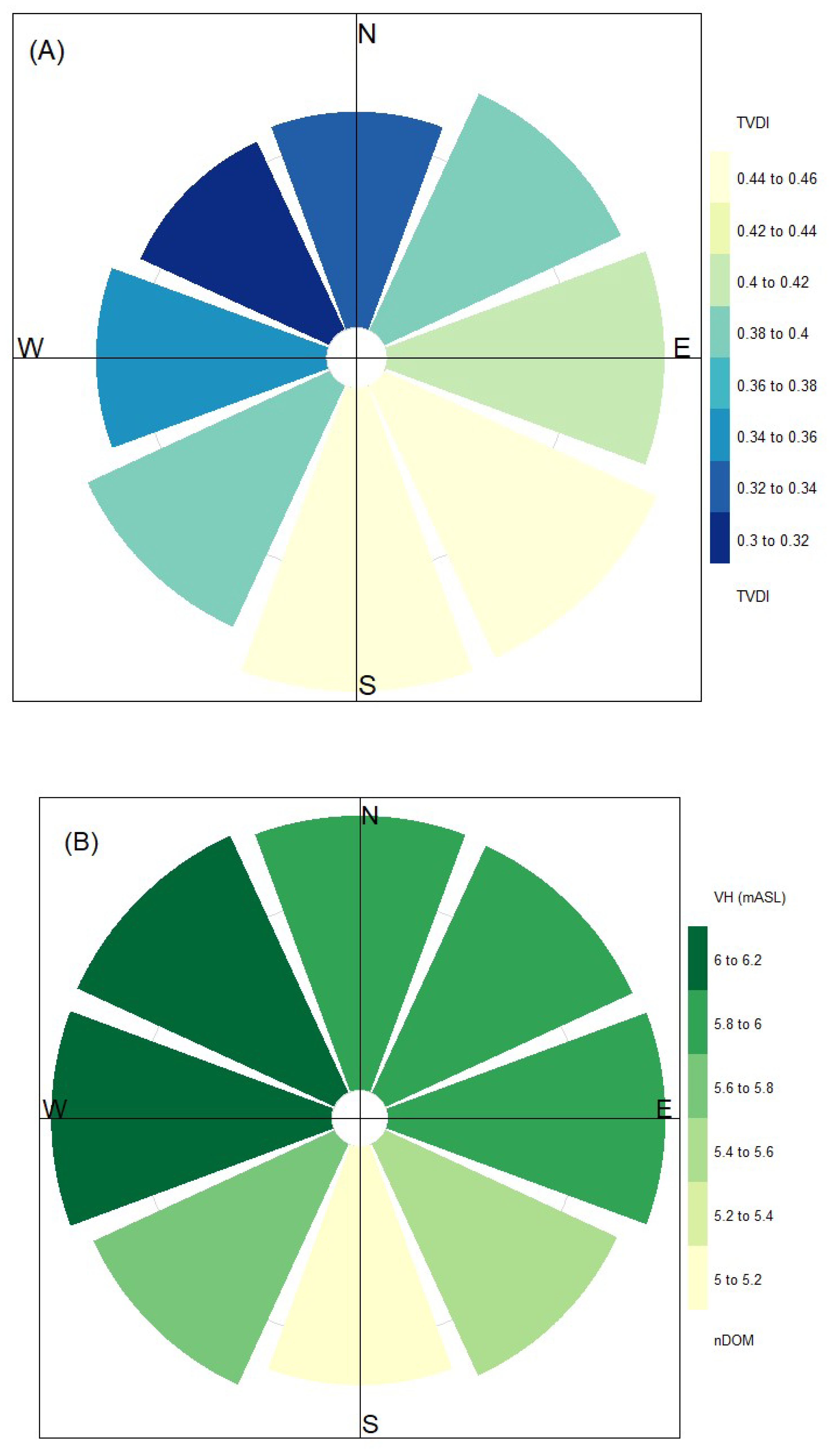
To identify more general relationships, mean TVDI pixel values from all Landsat summer scenes were analysed. To display their spatial distribution across all piles, TVDI and VH pixel mean values were grouped according to the eight main geographic directions (Figure 8).
Across all piles, mean TVDI values varied between 0.30 and 0.46, where the lowest values (moist soils) are found on the north and northwest slopes of the pile hills (Figure 8). Complementary to this, the highest values and thus soils with the lowest moisture were found in the south and southeast exposition of the piles. Interestingly, the spatial distribution of the mean TVDI seems to be more than a temporal snapshot since the mean TVDI directional values significantly correlated with the mean VH directional values (r = -0.8), which is also visualized in in Figure 8. Here, the highest vegetation heights are found on the northwest and west while the lowest occur on the south and southeast facing slopes. Apparently, soil moisture as a growth limiting factor is another indirect but important variable controlling the LST patterns on tailing piles.

4. Discussion

4.1. The Role of Tailing Piles as Cooling Urban Greens

Generally, tailing piles showed mean LSTs in a similar range as those of parks or allotment gardens across the Ruhr Area. While the role of these UGSs as cooling islands in UHI mitigation has been demonstrated in numerous studies, our study shows that rehabilitated tailing piles can be of similar significance. This is a more or less neglected phenomenon, resulting in a lack of comparable studies. To our knowledge, only the case study of Glocke et al. [45] analyzed the cooling potential of a tailing pile, also in the Ruhr Area. They showed that compared to flat urban parks such piles have an additional cooling potential during nighttime, because then cool air can drain down the slopes into adjacent residential areas. This highlights an aspect, which we couldn’t consider but which can additionally contribute to our documented potential of tailing piles to cool their immediate surroundings and thus provide an important ecosystem service.
The unique topography of tailing piles as hills in a rather flat surrounding is also partly responsible for their rather high variability in LST values compared to other UGSs. The influence of terrain factors on LST has also been studied by Mathew [72] and Tan et al. [34] [34,72], who generally explained this by terrain-dependent variation of solar incident radiation.

4.2. Factors Controlling LST on Tailing Piles

Cluster analyses based on the mean pile LST values showed that vegetation characteristics mainly differentiate the piles into four clusters. Interestingly, terrain attributes of the piles showed no statistically significant differences between the LST clusters. Similarly, the variability of mean pixel LST values across all piles was mainly explained by vegetation vitality indices (NDVI, NDMI) and vegetation height and far less by terrain factors in the RFR models, which reached up to 86% prediction accuracy. Similar strong relationships between LST and NDVI or NDMI values have been reported in numerous other studies because vegetation abundance and its moisture condition directly regulate the evaporative cooling processes [33]. Since the complex tailing pile environment shows a high heterogeneity of grass, shrub, and tree vegetation, both indices vary greatly and thus have a high impact on LST patterns. The fact that NDMI was more important than NDVI was also previously reported in several studies [33,34,35,73] and explained by the importance of plant available water as the limiting factor for transpirative cooling processes.
The influence of vegetation height on LST has been analyzed less often [74,75], most likely due to lack of available data from the expensive aerial laser scan campaigns. In a study by Chen et al. [76], the species composition of the tree canopy showed the highest impact on LST variability, but its vertical structure was also an important impact factor. Similar to our results, Gage and Cooper [77] found that NDVI played the most crucial role in explaining LST variability, but this was directly followed by tree height. They explained the additional impact of vegetation height on the LST pattern by shading effects on adjacent areas even when plant transpiration rates are low.
Contrary to our expectations, terrain attributes had only minor impacts on the summer LST patterns, although tailing piles generally have pronounced 3D hill shapes. The exposure to solar radiation and the associated effect on LST depends on elevation, aspect and steepness of slopes [41,78,79]. Due to the relatively small elevation differences of 50-150 m in our study area, this factor has little influence on LST. In our region where Landsat overpasses around early noon time, slope steepness in the range of >0° to 45° is positively related to the amount of direct solar radiation on south facing slopes, whereas the opposite is true for north facing slopes [78]. This opposing effect therefore likely masks the potential influence of slope in our regression analyses. While the impact of the aspect on the LST distribution was also negligible among all tailing piles, it increased substantially when only piles with elevations > 125 m were considered. At the relatively high solar azimuth angels of 60 to 63° for our summer satellite images, the incidence of sunlight was apparently impeded on north-exposed hillsides only of these higher tailing. For the winter image, aspect and the hillshade parameter modeled by ArcGIS became the most important controlling variables for LST because vegetation was bare or dormant, but also because the solar zenith angle drops to about 15° so that shading effects on slopes that are not exposed to the sun become more prominent, thus becoming an important factor for LST variability.
Studies like that of Bai et al. [41] or Karbalee et al. [40] which identified terrain attributes such as elevation, slope and aspect to control LST variability were generally conducted in natural mountainous areas where elevation differences were much greater and which are then associated with changes in the composition and density of the vegetation. The tailing piles are only low artificial hills with a man-made plant cover that was varied mainly for aesthetic reasons and is therefore not related to any terrain attributes.
Although the aspect parameter generally showed a low impact on the LST patterns, it was a relevant variable for describing the relationship between soil moisture estimated by the TVDI index and vegetation height. We observed that slopes with north-northwest exposition generally showed the lowest TVDIs i.e., highest soil moisture values, and accordingly, the greatest vegetation heights. Complementary, south, and southeast exposed hillsides generally showed low soil moisture, which most likely caused the lower vegetation heights. The effect of soil moisture variation on vegetation growth is well-known and is often a result of topographic variation [80,81,82]. Thus, studies frequently used the Topographic Wetness Index (TWI) to describe and predict vegetation height. For example, in the study of Mohamedou et al. [81] the TWI was used to improve the growth-prediction accuracy of LiDAR-based vegetation heights. However, to the best of our knowledge, the TVDI has never been used in this context. Unlike the TWI, the TVDI does not consider water movement in soils, but it appears to be a promising factor in predicting vegetation height, especially on tailing piles. Since the piles were constructed from fragmented bedrock debris, seepage water will most likely not move laterally downhill but will drain into the pile body, making it unavailable for plant roots, independent of slope position.

4.3. Implications for Urban Planning

Generally, the LST footprint of the tailing piles was found to be similar to those of other urban green spaces such as parks, cemeteries or allotments. Parks have been well characterized as effective cooling islands in numerous studies, so even for city residents, an awareness of their health-related benefits has been created [7]. Although the tailing piles in the Ruhr Area are used for local recreation, city residents are not aware of their cooling potential and their potential to improve healthy living conditions, especially during summertime. Thus, we advise urban planners to promote the remarkable benefit of the tailing piles as cooling islands to increase visitor numbers and improve the quality of urban life.
Within the tailing pile areas, the presence of taller vegetation and its moisture content were found to be the most important factors controlling LST variability during summer. Along south and southeast facing slopes, soil water availability limits tree growth and transpirational cooling. Increasing soil water capacity would thus increase the cooling potential of these expositions. This could be achieved during tailing pile rehabilitation by increasing the soil cover thickness or by selecting soil substrates with high soil water retention for these sites. On established vegetated piles, soil additives that provide high water capacities, such as organic mulches or biochar [83,84] could be spread out on the surfaces or mixed into the topsoil to achieve improvements of the cooling potential.
Another cooling feature of tailing piles that is not shared by other more flat urban green spaces is the downhill drainage of cool air into the surrounding neighborhoods during night, as described by Glocke et al. [45]. According to our data, this should be most pronounced along north and northwest facing slopes where daytime temperatures are lowest. Since this flux of cool air can easily be blocked by obstacles, such as walls or buildings at the hillfoot (Glocke et al. 2023), we advise urban planners to improve the pile cooling potential by removing barriers in the drainage pathways, especially in north and northwest expositions, to alleviate night-time urban heat in the surrounding neighborhoods.

4.4. Limitations and Open Questions

Many parts of this analysis are based on mean values from dates with warm to hot air temperatures, low cloud cover and no rainfall during the previous 2 weeks. This assures that the weather conditions were comparable across the whole study area before and during satellite imaging. However, the variability of LST within each UGS class und between the four UGS classes differed from date to date, indicating that season and other dynamic parameters such as soil moisture or plant phenology, possibly also management affect the cooling potential differently in the UGSs. Working with mean values allows for a better classification of the pile types, but masks temporal effects that may be relevant for LST variability at the local scale. On the other hand, the RFR models explaining the LST variability at the pixel level which are also based on mean values from the summer dates show a very good model performance, with R2 > 0.8 and low RMSE and MAE values. This indicates that temporal effects on the cooling potential of the tailing piles may be of minor importance. But this remains to be investigated.
Another flaw in the data analysis is based on the temporal incongruency between satellite scenes and the DEM and nDSM data. While the Landsat scenes stem from 2013 to 2023, the LiDAR campaigns were in 2019 and 2020. Since the rehabilitation of most tailing piles was completed before 2013 [85], the tree heights determined in 2019/20 may not be representative for the height distributions three to six years before this date. However, this was the best data available for the region and once again, the model performance based on the mean values from the satellite scenes indicate that the found relationships are solid and meaningful.
Finally, the LSTs of the tailing piles may not only originate from solar radiation but also from internal sources since several piles in the region contain patches of smoldering coal remains, leading to localized internal temperatures of 60 to 400°C (Kürten et al., 2014; Bezirksregierung Arnsberg, pers. comm.). But the effect of these smoldering patches on surface temperatures or their location and spatial extent are unknown and could only be estimated from night-time aerial or satellite imaging, which both are currently not available at the required spatial resolution. In any case, such “hot spots” can only have very minor effects on surface LST values since these are very well predicted from soil and vegetation parameters in our RFR models.

Author Contributions

Conceptualization, B.S. and B.M.; methodology, B.S..; validation, B.S. and B.M.; statistical analysis, B.S.; resources, B.S.; data curation, B.S.; writing—original draft preparation, B.S.; writing—review and editing, B.M.; visualization, B.S. All authors have read and agreed to the published version of the manuscript.

Funding

This research received no external funding.

Data Availability Statement

We encourage all authors of articles published in MDPI journals to share their research data. In this section, please provide details regarding where data supporting reported results can be found, including links to publicly archived datasets analyzed or generated during the study. Where no new data were created, or where data is unavailable due to privacy or ethical restrictions, a statement is still required. Suggested Data Availability Statements are available in section “MDPI Research Data Policies” at https://www.mdpi.com/ethics.

Acknowledgments

We would like to thank Thorsten Stock, Heiko Geyer and Carsten Lutter from the Ruhr Regional Association (RVR) for providing the shape files of the tailing pile delineations. This helped us greatly by ensuring that the data set was complete.

Conflicts of Interest

The authors declare no conflicts of interest.

Appendix A

Table A1. Characterization of the different selected Landsat scenes according to their cloud coverage and climatic condition before and while satellite overpassing. All scenes are from row 197, path 24 with C2L1, Tier1 data quality.
Preprints 118563 i004
Table A2. Characteristics of the four selected tailing piles that are representative for the clusters differentiated according to LST.
Preprints 118563 i005

References

  1. Yang, L. , Qian, F., Song, D.-X., Zheng, K.J. Research on urban heat-island effect. Procedia Engineering 2016, 169, 11–18. [Google Scholar] [CrossRef]
  2. Deilami, K.; Kamruzzaman, M.; Liu, Y. Urban heat island effect: A systematic review of spatio-temporal factors, data, methods, and mitigation measures. International Journal of Applied Earth Observation and Geoinformation 2018, 67, 30–42. [Google Scholar] [CrossRef]
  3. Oke, T.R. The Energetic Basis of the Urban Heat Island. Quarterly Journal of the Royal Meteorological Society 1982, 455, 1–24. [Google Scholar] [CrossRef]
  4. Aflaki, A. , Mirnezhad, M., Ghaffarianhoseini, A., Ghaffarianhoseini, A., Omrany, H., Wang, Z.-H., Akbari, H. Urban heat island mitigation strategies: A state-of-the-art review on Kuala Lumpur, Singapore and Hong Kong. Cities 2017, 62, 131–145. [Google Scholar] [CrossRef]
  5. Wang, Y. , Akbari, H. Analysis of urban heat island phenomenon and mitigation solutions evaluation for Montreal. Sustainable Cities and Society 2016, 26, 438–446. [Google Scholar] [CrossRef]
  6. O`Malley, C.; Piroozfar, P.; Farr, E.R.P.; Pomponi, F. Urban Heat Island (UHI) mitigating strategies: A case-based comparative analysis. Sustainable Cities and Society 2015, 19, 222–235. [Google Scholar] [CrossRef]
  7. Aram, F.; Higueras García, E.; Solgi, E.; Mansournia, S. Urban green space cooling effect in cities. Heliyon 2019, 5, 1–31. [Google Scholar] [CrossRef]
  8. Gago, E.J. , Roldan, J., Pacheco-Torres, R., Ordònez, J. The city and urban heat islands: A review of strategies to mitigate adverse effects. Renewable and Sustainable Energy Reviews 2013, 25, 749–758. [Google Scholar] [CrossRef]
  9. Mackey, C.W. , Lee, X., Smith, R.B. Remotely sensing the cooling effects of city scale efforts to reduce urban heat island. Build. Environ. 2012, 49, 348–358. [Google Scholar] [CrossRef]
  10. Farhadi, H. , Faizi, M., Sanaieian, H. Mitigating the urban heat island in a residential area in Tehran: Investigating the role of vegetation, materials, and orientation of buildings. Sustainable Cities and Society 2019, 46, 101448. [Google Scholar] [CrossRef]
  11. Lai, D. , Liu, W., Gan, T., Liu, K., Chen, Q. A review of mitigating strategies to improve the thermal environment and thermal comfort in urban outdoor spaces. Sci. Total Environ. 2019, 661, 337–353. [Google Scholar] [CrossRef] [PubMed]
  12. Norton, B.A. , Coutts, A.M., Livesley, S.J., Harris, R.J., Hunter, A.M., Williams, N.S.G. Planning for cooler cities: A framework to prioritise green infrastructure to mitigate high temperatures in urban landscapes. Landscape and Urban Planning 2015, 134, 127–138. [Google Scholar] [CrossRef]
  13. Sun, R. , Chen, L. Effects of green space dynamics on urban heat islands: Mitigation and diversification. Ecosystem Services 2017, 23, 38–46. [Google Scholar] [CrossRef]
  14. Stumpe, B. , Stuhrmann, N., Jostmeier, A., Marschner, B. Urban cemeteries: The forgotten but powerful cooling islands. The Science of the total environment 2024, 934, 173167. [Google Scholar] [CrossRef] [PubMed]
  15. Huang, C.; Huang, P.; Wang, X.; Zhuou, Z. Assessment and optimization of green space for urban transformation in resources-based city - A case study of Lengshuijiang city, China. Urban Forestry & Urban Greening 2018, 30, 295–306. [Google Scholar]
  16. Hamada, S.; Ohta, T. Seasonal variations in the cooling effect of urban green areason surrounding urban areas. Urban Forestry & Urban Greening 2010, 9, 15–24. [Google Scholar] [CrossRef]
  17. Kuang, W. , Liu, Y., Dou, Y., Chi, W., Chen, G., Gao, C., Yang, T., Liu, J., Zhang, R. What are hot and what are not in an urban landscape: quantifying and explaining the land surface temperature pattern in Beijing, China. Landscape Ecology 2015, 30, 357–373. [Google Scholar] [CrossRef]
  18. Algretawee, H. The effect of graduated urban park size on park cooling island and distance relative to land surface temperature (LST). Urban CLim. 2022, 45, 101255. [Google Scholar] [CrossRef]
  19. Park, S. , Im, J., Park, S., Rhee, J. Drought monitoring using high resolution soil moisture through multi-sensor satellite data fusion over the Korean peninsula. Agricultural and Forest Meteorology 2017, 237, 257–269. [Google Scholar] [CrossRef]
  20. Cao, X.; Onishi, A.; Chen, J.; Imura, H. Quantifying the cool island intensity of urban parks using ASTER and IKONOS data. Landscape and Urban Planning 2010, 96, 224–231. [Google Scholar] [CrossRef]
  21. Masoudi, M. , Tan, P.Y., Fadaei, M. The effects of land use on spatial pattern of urban green spaces and their cooling ability. Urban CLim. 2021, 35, 100743. [Google Scholar] [CrossRef]
  22. Kong, F.; Yin, H.; Wang, C.; Cavan, G.; James, P. A satellite image-based analysis of factors contributing to the green-space cool island intensity on a city scale. Urban Forestry & Urban Greening 2014, 13, 846–853. [Google Scholar] [CrossRef]
  23. Li, Y. , Ren, C., Ying-en Ho, J., Shi, Y. Landscape metrics in assessing how the configuration of urban green spaces affects their cooling effect: A systematic review of empirical studies. Landscape and Urban Planning 2023, 239, 104842. [Google Scholar] [CrossRef]
  24. Terfa, B.K. , Chen, N., Zhang, X., Niyogi, D. Spatial Configuration and Extent Explains the Urban Heat Mitigation Potential due to Green Spaces: Analysis over Addis Ababa, Ethiopia. remote sensing 2020, 12, 2876. [Google Scholar] [CrossRef]
  25. Yao, L. , Li, T., Xu, M., Xu, Y. How the landscape features of urban green space impact seasonal land surface temperatures at a city-block-scale: An urban heat island study in Beijing, China. Urban Forestry & Urban Greening 2020, 52, 126704. [Google Scholar] [CrossRef]
  26. Hou, H. , Estoque, R.C. Detecting Cooling Effect of Landscape from Composition and Configuration: An Urban Heat Island Study on Hangzhou. Urban Forestry & Urban Greening 2020, 53, 126719. [Google Scholar] [CrossRef]
  27. Amani-Beni, M.; Zhang, B.; Xie, G.D.; Xu, J. Impact of urban park's tree, grass and waterbody on microclimate in hot summer days: A case study of Olympic Park in Beijing, China. Urban Forestry & Urban Greening 2018, 32, 1–6. [Google Scholar] [CrossRef]
  28. Wang, X.; Dallimer, M.; Scott, C.E.; Shi, W.; Gao, J. Tree species richness and diversity predicts the magnitude of urban heat island mitigation effects of greenspaces. The Science of the total environment 2021, 770, 1–42. [Google Scholar] [CrossRef]
  29. Rahman, M.A. , Armson, D., Ennos, A.R. A comparison of the growth and cooling effectiveness of five commonly planted urban tree species. Urban Ecosystems 2015, 18, 371–389. [Google Scholar] [CrossRef]
  30. Helletsgruber, C. , Gillner, S., Gulyas, A., Junker, R.R., Tanacs, E., Hof, A. Identifying Tree Traits for Cooling Urban Heat Islands—A Cross-City Empirical Analysis. Forests 2020, 11, 1064. [Google Scholar] [CrossRef]
  31. Kong, F. , Yan, W., Zheng, G., Yin, H., Cavan, G., Zhan, W., Zhang, N., Cheng, L. Retrieval of three-dimensional tree canopy and shade using terrestrial laser scanning (TLS) data to analyze the cooling effect of vegetation. Agricultural and Forest Meteorology 2017, 217, 22–34. [Google Scholar] [CrossRef]
  32. Wang, X. , Rahman, M.A., Mokros, M., Rötzer, T., Pattnaik, N., Pang, Y., Zhang, Y., Da, L., Song, K. The influence of vertical canopy structure on the cooling and humidifying urban microclimate during hot summer days. Landscape and Urban Planning 2023, 238, 104841. [Google Scholar] [CrossRef]
  33. Stumpe, B.; Bechtel, B.; Heil, J.; Jörges, C.; Jostmeier, A.; Kalks, F.; Schwarz, K.; Marschner, B. Soil texture mediates the surface cooling effect of urban and peri-urban green spaces during a drought period in the city area of Hamburg (Germany). Sci. Total Environ. 2023, 897, 165228. [Google Scholar] [CrossRef] [PubMed]
  34. Tan, J.; Yu, D.; Li, Q.; Tan, X.; Zhou, W. Spatial relationship between land-use/land-cover change and land surface temperature in the Dongting Lake area, China. Scientific reports 2020, 10, 1–9. [Google Scholar] [CrossRef]
  35. Le, M.S. , Liou, Y.-A. Spatio-Temporal Assessment of Surface Moisture and Evapotranspiration Variability Using Remote Sensing Techniques. Remote Sensing 2021, 13, 1667. [Google Scholar] [CrossRef]
  36. Sandholt, I. , Rasmussen, K., Andersen, J. A simple interpretation of the surface temperature/vegetation index space for assessment of surface moisture status. Remote Sensing of Environment 2002, 79, 213–224. [Google Scholar] [CrossRef]
  37. Chen, J. , Wang, C., Jiang, H., Mao, L., Zhenrong, Y. Estimating soil moisture using Temperature–Vegetation Dryness Index (TVDI) in the Huang huai-hai (HHH) plain. International Journal of Remote Sensing 2011, 32, 1165–1177. [Google Scholar] [CrossRef]
  38. Yuan, L., Li, L., Zhang, T., Chen, L., Zhao, J., Hu, S., Cheng, L., Liu, W. Soil Moisture Estimation for the Chinese Loess Plateau Using MODIS-derived ATI and TVDI. Remote Sensing 12, 3040. [CrossRef]
  39. Zhao, H. , Li, Y., Chen, X., Wang, H., Yao, N., Liu, F. Monitoring monthly soil moisture conditions in China with temperature vegetation dryness indexes based on an enhanced vegetation index and normalized difference vegetation index. Theoretical and Applied Climatology 2021, 143, 159–176. [Google Scholar] [CrossRef]
  40. Karbalaee, A.R. , Hedjazizadeh, Z., Masoodian, S.A. Dependency of LSA and LST to topographic factors in Iran, based on remote sensing data. Theoretical and Applied Climatology 2023, 153, 709–726. [Google Scholar] [CrossRef]
  41. Bai, Y. , Wang, K., Ren, Y., Li, M., Ji, R., Wu, X., Yan, X., Lin, T., Zhang, G., Zhou, X., Mei, H., Ye, H. 3D compact form as the key role in the cooling effect of greenspace landscape pattern. Ecological Indicators 2024, 160, 111776. [Google Scholar] [CrossRef]
  42. Cao, X. , Onishi, A., Chen, J., Imura, H. Quantifying the cool island intensity of urban parks using ASTER and IKONOS data. Landscape and Urban Planning 2010, 96, 224–231. [Google Scholar] [CrossRef]
  43. Spronken-Smith, R.A. , Oke, T.R. The thermal regime of urban parks in two cities with different summer climates. International Journal of Remote Sensing 1998, 19, 2085–2104. [Google Scholar] [CrossRef]
  44. Okumus, E.E.; Terzi, F. Ice floes in urban furnance: Cooling services of cemeteries in regulating the thermal environment of Istanbul`s urban landscape. Urban CLim. 2023, 49, 101549. [Google Scholar] [CrossRef]
  45. Glocke, P. , Scholz, T., Grudzielanek, M.A. Assessing the Cooling Potential of Tailing Piles for Urban Heat Mitigation in Germany’s Ruhr Metropolitan Area—A Case Study of the Rungenberg in Gelsenkrichen. Atmosphere 2023, 14, 1492. [Google Scholar] [CrossRef]
  46. Goetzke, R., Over, M., Braun, M. A METHOD TO MAP LAND-USE CHANGE AND URBAN GROWTH IN NORTH RHINE-WESTPHALIA (GERMANY). Proceedings of the 2nd Workshop of the EARSeL SIG on Land Use and Land Cover 2006, 102-111.
  47. Auer, S.; Wenning, T.; Burk, B.; Mathee-Will, G.; Müller, H.C. People. Nature. Space. Green infrastructure in the Ruhr metropolis.; Regionalverband Ruhr: Essen, Germany, 2021; p. 33.
  48. Schulz, D. Recultivation of mining waste dumps in the Ruhr Area, Germany. In Minesite Recultivation, Reinhard, F.H., Heinkele, T., Wisniewski, J., Ed.; Springer: 1996; pp. 89–98.
  49. Schulz, D. Recultivation of mining waste dumps in the Ruhr Area, Germany. Water, Air, and Soil Pollution 1996, 91, 89–98. [Google Scholar] [CrossRef]
  50. Bezirksregierung-Koeln. Digitales Basis-Landschaftsmodell - Paketierung: gesamt NRW. Available online: https://www.opengeodata.nrw.de/produkte/geobasis/lm/akt/basis-dlm/ (accessed on June 2024).
  51. USGS. EarthExplorer. Available online: https://earthexplorer.usgsgov/ (accessed on.
  52. Avdan, U.; Jovanovska, G. Algorithm for Automated Mapping of Land Surface Temperature Using LANDSAT 8 Satellite Data. Journal of Sensors 2016, 2016, 1–8. [Google Scholar] [CrossRef]
  53. Stathopoulou, M.C. Daytime urban heat island from Landsat ETM+ and Corine land cover data: An application to major cities in Greece. Solar Energy 2007, 81, 358–368. [Google Scholar] [CrossRef]
  54. Huang, S.; Tang, L.; Hupy, J.P.; Wang, Y.; Shao, G. A commentary review on the use of normalized difference vegetation index (NDVI) in the era of popular remote sensing. Journal of Forest Research 2021, 32, 1–6. [Google Scholar] [CrossRef]
  55. Burnett, M.; Chen, D. Urban Heat Island Footprint Effects in Bio-Productive Rural Land Covers Surrounding a Low Density Urban Center. The International Archives of the Photogrammetry, Remote Sensing and Spatial Information Sciences 2021, Volume XLIII-B3-2021, 539–550.
  56. Taloor, A.K.; Manhas, D.S.; Kothyari, G.C. Retrieval of land surface temperature, normalized difference moisture index, normalized difference water index of the Ravi basin using Landsat data. Appl. Comput. Geosci. 2021, 9, 11. [Google Scholar] [CrossRef]
  57. Yu, Z.; Guo, X.; Jørgensen, G.; Vejre, H. How can urban green spaces be planned for climate adaptation in subtropical cities? Ecological Indicators 2017, 82, 152–162. [Google Scholar] [CrossRef]
  58. Halder, B.; Karimi, A.; Mohammad, P.; Bandyopadhyay, J.; Brown, R.D.; Yaseen, Z.M. Investigating the relationship between land alteration and the urban heat island of Seville city using multi-temporal Landsat data. Theoretical and Applied Climatology 2022, 150, 613–635. [Google Scholar] [CrossRef]
  59. Hoffmann, T. SunCalc. Available online: https://www.suncalc.org (accessed on.
  60. Heil, H.; Häring, V.; Marschner, B.; Stumpe, B. Advantages of fuzzy k-means over k-means clustering in the classification of diffuse reflectance soil spectra: A case study with West African soils. Geoderma 2019, 337, 11–21. [Google Scholar] [CrossRef]
  61. Kodinariya, T.; Makwana, P. Review on determining of cluster in K-means clustering. International Journal of Applied Earth Observation and Geoinformation 2013, 1, 90–95. [Google Scholar]
  62. MacQueen, J. Some methods for classification and analysis of multivariate observations. Proceedings of the fifth Berkeley symposium on mathematical statistics and probability. 1967, 1(14), 281–297. [Google Scholar]
  63. R_foundation. The R Project for Statistical Computing. Available online: https://www.r-project.org/ (accessed on March 20, 2024).
  64. Kassambara, A.; Mundt, F. Factoextra: Extract and Visualize the Results of Multivariate Data Analyses. R Package Version 1.0.7. Available online: https://CRAN.R-project.org/package=factoextra (accessed on March 30, 2024).
  65. Breimann, L. Random Forest. Machine Learning 2001, 45, 5–32. [Google Scholar] [CrossRef]
  66. Jörges, C.; Berkenbrink, C.; Stumpe, B. Prediction and reconstruction of ocean wave heights based on bathymetric data using LSTM neural networks. Ocean Engeneering 2021, 232. [Google Scholar] [CrossRef]
  67. Liaw, A.; Wiener, M. Classification and Regression by Randomforest. R News 2002, 2, 18–22. [Google Scholar]
  68. Fox, E.W.; Hill, R.A.; Leibowitz, S.; Olsen, A.R.; Thornbrugh, D.J.; Weber, M.H. Assessing the accuracy and stability of variable selection methods for random forest modeling in ecology. Environmental Monitoring Assessment 2017, 189(7), 316. [Google Scholar] [CrossRef]
  69. Kuhn, S.; Egert, B.; Neumann, S.; Steinbeck, C. Building blocks for automated elucidation of metabolites: Machine learning methods for NMR prediction. BMC Bioinformatics 2008, 9, 1–19. [Google Scholar] [CrossRef] [PubMed]
  70. Mirchooli, F.; Kiani-Harchegani, M.; Darvishan, A.K.; Falahatkar, S.; Sadeghi, S.H. Spatial distribution dependency of soil organic carbon content to important environmental variables. Ecological Indicators 2020, 116, 106473. [Google Scholar] [CrossRef]
  71. Hamner, B. Metrics. Available online: https://github.com/mfrasco/Metrics/tree/master/R (accessed on.
  72. Mathew, A. , Khandelwal, S., Kaul, N. Spatial and temporal variations of urban heat island effect and the effect of percentage impervious surface area and elevation on land surface temperature: Study of Chandigarh city, India. Sustainable Cities and Society 2016, 26, 264–277. [Google Scholar] [CrossRef]
  73. Macarof, P.; Bartic, G.C.; Groza, S.; Statescu, F. ANALYSIS OF LST-NDVI SPARSE/DENSE VEGETATION RELATIONSHIP: A CASE STUDY OF IASI COUNTY. Sci. Pap.-Ser. E-Land Reclam. Earth Obs. Surv. Environ. Eng. 2018, 7, 168–173. [Google Scholar]
  74. Yang, C.; He, X.; Wang, R.; Yan, F.; Yu, L.; Bu, K.; Yang, J.; Chang, L.; Zhang, S. The Effect of Urban Green Spaces on the Urban Thermal Environment and Its Seasonal Variations. Forests 2017, 8, 1–19. [Google Scholar] [CrossRef]
  75. Caynes, R.J.C. , Mitchell, M.G.E., Sabrina, D., Johansen, K., Rhodes, J.R. Using high-resolution LiDAR data to quantify the three-dimensional structure of vegetation in urban green space. Urban Ecosystems 2016, 19, 1749–1765. [Google Scholar] [CrossRef]
  76. Chen, J.; Jin, S.; Du, P. Roles of horizontal and vertical tree canopy structure in mitigating daytime and nighttime urban heat island effects. International Journal of Applied Earth Observation and Geoinformation 2020, 89, 1–11. [Google Scholar] [CrossRef]
  77. Gage, E.A. , Cooper, D.J. Urban forest structure and land cover composition effects on land surface temperature in a semi-arid suburban area. Urban Forestry & Urban Greening 2017, 28, 28–35. [Google Scholar] [CrossRef]
  78. Keating, K.A.; Gogan, P.J.P.; Vore, J.M.; Irby, L.R. A Simple Solar Radiation Index for Wildlife Habitat Studies. Journal of Wildlife Management 2020, 71, 1344–1348. [Google Scholar] [CrossRef]
  79. Peng, X.; Wu, W.; Zheng, Y.; Sun, J.; Hu, A.; Wang, P. Correlation analysis of land surface temperature and topographic elements in Hangzhou, China. Scientific Reports 2020, 10, 10451. [Google Scholar] [CrossRef] [PubMed]
  80. Anning, A.K. , Rubino, D.L., Sutherland, E.K., McCarthy, B.C. Dendrochronological analysis of white oak growth patterns across a topographic moisture gradient in southern Ohio. Dendrochronologia 2013, 31, 120–128. [Google Scholar] [CrossRef]
  81. Mohamedou, C. , Tokola, T., Eerikäinen, K. LiDAR-based TWI and terrain attributes in improving parametric predictor for tree growth in southeast Finland. International Journal of Applied Earth Observation and Geoinformation 2017, 62, 183–191. [Google Scholar] [CrossRef]
  82. Adams, H.R. , Barnard, H.R., Loomis, A.K. Topography alters tree growth–climate relationships in a semi-arid forested catchment. Ecosphere 2014, 5, 148. [Google Scholar] [CrossRef]
  83. Tanure, M.M.C. , Costa, L.M., Huiz, H.A., Fernandes, R.B.A., Cecon, P.R., Junior, J.D.P., de Luz, J.M.R. Soil water retention, physiological characteristics, and growth of maize plants in response to biochar application to soil. Soil & Tillage Research 2019, 192, 164–173. [Google Scholar] [CrossRef]
  84. Atkinson, C.J. How good is the evidence that soil-applied biochar improves water-holding capacity? Soil Use and Management 2018, 34, 177–186. [Google Scholar] [CrossRef]
  85. Kürten, S.; Feindegen, M.; Noel, Y. Geothermal Utilization of Smoldering Mining Dumps. In Coal and Peat Fires: A Global Perspective, Stracher, G.B., Prakash, A., Sokol, E.V., Eds.; Elsevier: 2015; Volume 4, pp. 241–261.
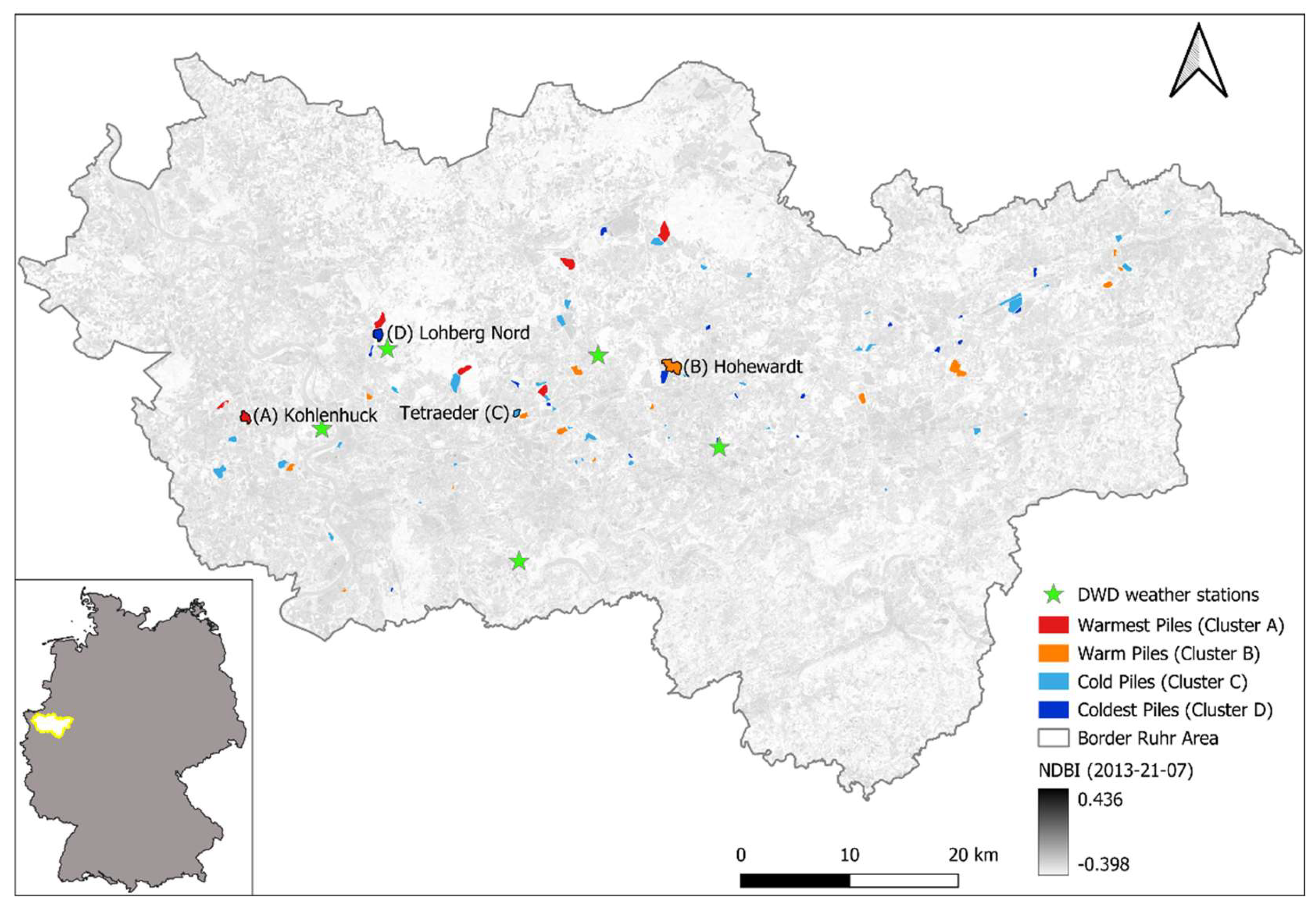
Figure 1. Distribution of the tailing piles across the Ruhr Area, differentiated according to the four LST clusters (see Section 3.2). The basemap is the NDBI (Normalized Different Built-up Index) based on the LANDSAT scene from July 21, 2013. The green stars show the locations of the DWD weather stations used for climatic characterization of the LANDSAT scene dates used for analyses.
Preprints 118563 g001
Figure 2. Histogram of the slope (°) (A), aspect (circular) (B), vegetation height as nDSM (m) (C) values across all tailing piles.
Preprints 118563 g002aPreprints 118563 g002b
Figure 3. Histogram of the summer mean LST values (°C) across all tailing piles (A) and the directional distribution of the mean summer LST for all tailing piles (B).
Preprints 118563 g003
Figure 4. Total variance within each cluster as a function of number of clusters. The dotted line indicates the optimum number of cluster as elbow of the curve (A) and the visualization of cluster separation along the two main dimensions.
Preprints 118563 g004
Figure 5. Representative tailing piles (Kohlenhuck, Hohewardt, Tetraeder, Lohberg Nord) for the four different thermal clusters (A-D) shown as orthophotos (first column), altitude (second column) and land surface temperature (third column).
Preprints 118563 g005
Figure 6. Variable importance (IncNodeMSE) for the random forest regression (RFR) models based on the summer (A) and winter (B) data sets. Results are shown for the whole summer and winter data sets (all) as well as for data sets separated according the tailing pile heights.
Preprints 118563 g006
Figure 8. Directional distribution of mean TVDI values (A) and vegetation heights (B) along the slopes of all tailing piles.
Preprints 118563 g008
Table 1. Characterization of the Urban Green Spaces (UGS) in the Ruhr area in terms of size and area as well as mean land surface temperatures (LST) determined from thermal satellite images at five different summer dates.
Preprints 118563 i001
Table 2. Cluster separation quality and characterization of the different thermal clusters according terrain, vegetation and soil attributes.
Preprints 118563 i002
Table 3. Model performance of the different Random Forest Regression models for explaining the variability of mean LST values at the pixel level, separated for summer and winter months.
Preprints 118563 i003
Disclaimer/Publisher’s Note: The statements, opinions and data contained in all publications are solely those of the individual author(s) and contributor(s) and not of MDPI and/or the editor(s). MDPI and/or the editor(s) disclaim responsibility for any injury to people or property resulting from any ideas, methods, instructions or products referred to in the content.
Copyright: This open access article is published under a Creative Commons CC BY 4.0 license, which permit the free download, distribution, and reuse, provided that the author and preprint are cited in any reuse.
Prerpints.org logo

Preprints.org is a free preprint server supported by MDPI in Basel, Switzerland.

Subscribe

© 2024 MDPI (Basel, Switzerland) unless otherwise stated