A State-Space Analysis and an Optimal Control Synthesis for a Class of Linear Time-Optimal Control Problems

Preprint

Article

A State-Space Analysis and an Optimal Control Synthesis for a Class of Linear Time-Optimal Control Problems

Altmetrics

Downloads

Views

114

Comments

Borislav Penev^*

This version is not peer-reviewed

Submitted:

18 September 2024

Posted:

20 September 2024

You are already at the latest version

Alerts

Abstract

The paper deals with two new properties of the linear time-optimal control problems with real non-positive eigenvalues of the system. They are the foundation of a new method of synthesizing the time-optimal control without the need to describe the switching hyper-surfaces. The so called “axes initialization” and the synthesis technique are illustrated on the already classical example of the time-optimal control of a double integrator.

Keywords:

Subject: Engineering - Control and Systems Engineering

1. Introduction

In [1] a new property of the linear time-optimal control problem for the case of real non-positive eigenvalues of the system is derived. In Section 4 – Discussion [1] (p. 13) it is said that „Besides the property proved here, there is still a rigorous need to prove other properties of the problem in the case of its expansion.“ The necessary theoretical elements of the new method include the questions about the relationship between the coordinate axes in the state-space of the system of the considered Problem P

(n)

and its switching hyper-surface, as well as the synthesis of the optimal control based on the solution of the easier Problem P

(n - 1)

generated by the original Problem P

(n) .

The present work is a direct continuation of the previous work [1] and deals precisely with these necessary theoretical questions. It should be noted that in the period since the publication of the previous work [1], there are no other published studies on the linear time-optimal control problem developing the idea of the proposed method.

Works [2] – [5] consider time-optimal trajectory planning of systems in the presence of limitations or time-varying parameters. They apply Pontryagin's maximum principle with still other optimization techniques. In [2] (p. 506) it is stated that „In control engineering, effective implementations require to take into account the constraints for both the inputs and the outputs of the controlled system.“ Some of the studies [2] – [4] on time-optimal control of linear systems with constraints offer solutions where “the proposed idea is to discretize the continuous-time system and to solve the resulting discrete-time problem by means of linear programming.” ([4], p. 2234) so that “By time discretization and linear programming, an approximation of the generalized bang-bang control can be computed.” [2] (p. 511). In [6] (p. 2) the authors note: „We observe that for many systems, time-optimal trajectories can be represented as a concatenation of multiple trajectory segments. … Take a double integrator as an example. It is well-known that its optimal control policy is bang-bang with at most one switch“. The direction of their research leads to „a polynomial-based quadrotor motion planner that can generate time-optimal trajectories for a wide range of scenarios“ [6] (p. 17). In [4] (p. 2234) it is noted that „in the control engineering literature, it has been emphasized that to achieve high performances in real applications, due attention has to be paid to the constraints which all the plant variables must comply with.“ The development and the maturity reached in the theory of time-optimal control [7] – [15] as well as the contribution of the contemporary researchers [16] – [18], [2] – [6] are a direct confirmation of the long-standing efforts in this field. The research in this field is accompanied and enriched in the years of its development and with theoretical attempts to justify the existence of closed-loop time-optimal control [19], [20]. The difficulties in this topic are reason to note that “… there is still no complete time-optimal analytical solution for systems higher than second order” [18] (p. 1). The approach of the authors of [18] (pp. 1–2) „can be considered in two steps: (1) the time optimal control of multiple integrator with only input saturation; (2) the time optimal control of multiple integrator with input saturation and full state constraints“. For their research „based on Bellman’s principle of optimality, a series of switching surfaces and curves in phase space is generated using dynamic programming method“ (p. 8).

The approach chosen in [1] and developed in the present work with regard to the classical linear time-optimal control problem of a controllable linear system with one input and real non-positive eigenvalues is based on the following main ideas:

Pontryagin's original solution [9] (Chapter 3, § 20, § 21, Example 3) with regard to the synthesizing function

u (x) = \{\begin{matrix} + 1 & i n a l l a r e a s & M_{i}^{+}, \\ - 1 & i n a l l a r e a s & M_{i}^{-}, \end{matrix}

where

M_{i}^{+}

and

M_{i}^{-}

are the respective manifolds. The manifold

M_{i}

is of dimension

(n - i + 1)

;

M_{i + 1}

is entirely in

M_{i}

and divides it into two areas

M_{i}^{+}

and

M_{i}^{-}

;

M_{i}^{+}

consists of all the trajectories under the control

+ 1

ending at a point of

M_{i + 1}^{-}

, while

M_{i}^{-}

consists of all the trajectories under the control

- 1

ending at a point of

M_{i + 1}^{+}

. The last manifold

M_{1}

coincides with the whole state-space of the system;

New geometric properties of the original time-optimal control problem with respect to the system state-space;

Solution of the synthesis problem based on the new properties of the time-optimal control problem and carried out without the need to describe or generate the respective manifolds – the switching hyper-surfaces, but by solving the simpler lower-order problem generated by the original time-optimal control problem.

The current paper is organized in the following way. In Section 2 two new properties of the linear time-optimal control problem are theoretically represented. In Section 3 the author carries out the so called "axes initialization" of the time-optimal control problem of a double integrator as well as the synthesis of the optimal control and obtaining the optimal trajectory. Section 4 presents some concluding remarks on the obtained results.

2. Formulation of the Problem and Solution

Let us consider the linear time-optimal control problem of order

n

n \geq 2

, called Problem P

(n)

as well as its sub-problem Problem P

(n - 1)

presented in [1] (pp. 2–4).

We have obtained that in the

n

-dimensional state-space of Problem P

(n)

the difference between the vector-function

x (t)

(28) of [1] with an initial point representing the initial state

x_{0}

(2) or (12) of [1] of Problem P

(n)

under the optimal control

u_{n - 1}^{o} (t), t \in [0, t_{(n - 1) f}^{o}],

of Problem P

(n - 1)

and the vector-function

x^{1} (t)

with an initial point

x_{0}^{1}

(20) – (21) of [1] under the optimal control

u_{n - 1}^{o} (t), t \in [0, t_{(n - 1) f}^{o}],

of Problem P

(n - 1)

represents (31) of [1]:

x (t) - x^{1} (t) = (\begin{matrix} {(\underset{n - 1}{\underset{⏟}{\begin{matrix} 0 & \dots & 0 \end{matrix}}})}^{T} \\ e^{λ_{n} t} (x_{n 0} {- x}_{n 0}^{1}) \end{matrix}) for t \in [0, t_{(n - 1) f}^{o}]

(1)

Let us continue the consideration of the second case of (31) of [1] or the above expression with regard to its last

n

-th coordinate

e^{λ_{n} t} (x_{n 0} {- x}_{n 0}^{1})

for

t \in [0, t_{(n - 1) f}^{o}]

, i.e. when

x_{n 0} {\neq x}_{n 0}^{1}

. In case

x_{n 0} {- x}_{n 0}^{1} > 0

(2)

and

x_{n 0}

describes sequentially all the values of the interval

{(x}_{n 0}^{1}, \infty)

, then by (31) of [1] all the points of the line passing through the point

x_{0}^{1}

with coordinates (20) – (21) of [1] parallel to the axis

{О x}_{n}

and located above the point

x_{0}^{1}

by (31) are transformed at the moment

t_{(n - 1) f}^{o}

successively into the points of the positive part of the axis

{О x}_{n}

of the

n

-dimensional state-space of Problem P

(n)

, whereby all these trajectories are located outside the switching hyper-surface of Problem P

(n)

having one and the same relation to it, simultaneously above or simultaneously below the switching hyper-surface of Problem P

(n)

. Thus the positive semi-axis

{О x}_{n}

is outside the switching hyper-surface of Problem P

(n)

, being wholly below or wholly above the switching hyper-surface of Problem P

(n)

. When

x_{n 0} {- x}_{n 0}^{1} < 0

(3)

based on the same reasoning we get that the negative semi-axis

{О x}_{n}

is outside the switching hyper-surface of Problem P

(n)

, being wholly below or wholly above the switching hyper-surface of Problem P

(n)

but in the opposite relation to the switching hyper-surface of Problem P

(n)

relative to the positive semi-axis

{О x}_{n} .

Based on this conclusion for the considered class of problems we could define the term for the variable

x_{n +}

spreading the definition of the term about the variable

x_{k +}

mentioned in [1] (p. 11) as a term introduced in [14] of [1] (p. 38) and [15] of [1] (pp. 319–320) “which defines the relation of the points of the axis

x_{k}

of the state-space of the system of Problem P

(k)

from the considered class of problems to the switching hyper-surface of the same Problem P

(k)

.”

Definition. We define

x_{n +}

as a variable accepting values

+ 1

- 1

, i.e.

x_{n +} \in \{\begin{matrix} - 1, & + 1 \end{matrix}\},

(4)

so that for the optimal control – the solution of Problem P

(n)

it must be satisfied:

\begin{matrix} u^{o} (0) = u_{0} & w h e n & \begin{array}{l} x_{0} = {(\begin{matrix} x_{10} \dots & x_{(n - 1) 0} & x_{n 0} \end{matrix})}^{T} \\ = {(\begin{matrix} \underset{n - 1}{\underset{⏟}{\begin{matrix} 0 & \dots & 0 \end{matrix}}} & x_{n 0} \end{matrix})}^{T}, x_{n 0} : s i g n (x_{n 0}) = x_{n +} . \end{array} \end{matrix}

(5)

As it is mentioned in [1] (p. 11) the value of the variable

x_{k +}

is determined by a procedure called “axes initialization” [14] of [1] (Chapter 3, Section 3.3, pp. 60–88), [16] of [1] (pp. 41–45).

In order to determine

x_{n +}

, let us now perform the following few constructions.

Construction 1

First, let us first choose

(n - 1)

random positive finite numbers

t_{1}

t_{2}

, …,

t_{(n - 1)}

, i.e.

t_{i} \in (0, \infty) for i = 1, 2, \dots, (n - 1)

(6)

Let us form the following piecewise constant function

u_{1} (t)

as an admissible function for the considered class of problems in [1] – “the admissible control

u (t)

is a piecewise continuous function that takes its values from the range (3), which is continuous on the boundaries of the set of allowed values (3) and in the points of discontinuity

τ

we have (4)”, where its value in the

i

-th interval,

i = 1, 2, \dots, (n - 1)

, is

u_{1} (t) = {(- 1)}^{i} u_{0} when t \in [\sum_{j = 1}^{i - 1} t_{j}, \sum_{j = 1}^{i} t_{j}) for i = 1, 2, \dots, (n - 1)

(7)

Note that the value of

u_{1} (t)

in the first interval of constancy is

- u_{0}

Let us denote by

t_{(n - 1) f}^{1}

the length of the function

u_{1} (t)

or the sum of the lengths of all intervals of constancy of

u_{1} (t)

t_{(n - 1) f}^{1} = \sum_{i = 1}^{(n - 1)} t_{i}

(8)

Let the initial state of Problem P

(n - 1)

be the following point

x_{(n - 1) 0}^{1}

in the

(n - 1)

-dimensional state-space of Problem P

(n - 1)

x_{(n - 1) 0}^{1} = - e^{{- A}_{n - 1} t_{(n - 1) f}^{1}} \int_{0}^{t_{(n - 1) f}^{1}} e^{A_{n - 1} (t - τ)} B_{n - 1} u_{1} (t) d τ

(9)

Let us now consider the trajectory in the

(n - 1)

-dimensional state-space of Problem P

(n - 1)

with an initial state

x_{(n - 1) 0}^{1}

(9) under the control

u_{1} (t)

(7)

x_{n - 1}^{1} (t) = e^{A_{n - 1} t} x_{(n - 1) 0}^{1} + \int_{0}^{t} e^{A_{n - 1} (t - τ)} B_{n - 1} u_{1} (t) d τ for t \in [0, t_{(n - 1) f}^{1}]

(10)

It is easy seen that the control

u_{1} (t)

(7) transfers the initial state

x_{(n - 1) 0}^{1}

(9) of the system of Problem P

(n - 1)

, (7) of [1], at the moment

t_{(n - 1) f}^{1}

at the origin of the

(n - 1)

-dimensional state-space of Problem P

(n - 1)

x_{n - 1}^{1} (t_{(n - 1) f}^{1}) = e^{A_{n - 1} t_{(n - 1) f}^{1}} x_{(n - 1) 0}^{1} + \int_{0}^{t_{(n - 1) f}^{1}} e^{A_{n - 1} (t - τ)} B_{n - 1} u_{1} (t) d τ

(11)

\begin{array}{l} x_{n - 1}^{1} (t_{(n - 1) f}^{1}) \\ = e^{A_{n - 1} t_{(n - 1) f}^{1}} (- e^{{- A}_{n - 1} t_{(n - 1) f}^{1}} \int_{0}^{t_{(n - 1) f}^{1}} e^{A_{n - 1} (t - τ)} B_{n - 1} u_{1} (t) d τ) \\ + \int_{0}^{t_{(n - 1) f}^{1}} e^{A_{n - 1} (t - τ)} B_{n - 1} u_{1} (t) d τ; \end{array}

(12)

\begin{matrix} x_{n - 1}^{1} (t_{(n - 1) f}^{1}) & = - I_{n - 1} \int_{0}^{t_{(n - 1) f}^{1}} e^{A_{n - 1} (t - τ)} B_{n - 1} u_{1} (t) d τ \\ + \int_{0}^{t_{(n - 1) f}^{1}} e^{A_{n - 1} (t - τ)} B_{n - 1} u_{1} (t) d τ; \end{matrix}

(13)

x_{n - 1}^{1} (t_{(n - 1) f}^{1}) = {(\underset{n - 1}{\underset{⏟}{\begin{matrix} 0 & \dots & 0 \end{matrix}}})}^{T}

(14)

Thus we can draw the following conclusion.

Corollary 1. The piecewise constant function

u_{1} (t)

(7) with an amplitude

u_{0}

(n - 1)

non-zero intervals of constancy

t_{1}

t_{2}

, …,

t_{(n - 1)}

, and a value in the first interval of constancy

- u_{0}

transfers the system of Problem P

(n - 1)

from its initial state

x_{(n - 1) 0}^{1}

(9) at the final moment

t_{(n - 1) f}^{1}

(8) at the origin of the

(n - 1)

-dimensional state-space of Problem P

(n - 1) .

The function

u_{1} (t)

represents the optimal control of Problem P

(n - 1)

with an initial state of the system

x_{(n - 1) 0}^{1}

. The point

x_{(n - 1) 0}^{1}

is located outside the switching hyper-surface of Problem P

(n - 1)

Let us denote by

y_{n - 1}^{1} (t)

the output of the system of Problem P

(n - 1)

, (7) of [1], with an initial state

x_{(n - 1) 0}^{1}

(9) under the control

u_{1} (t)

(7) for

t \in [0, t_{(n - 1) f}^{1}] :

y_{n - 1}^{1} (t) = C_{n - 1} x_{n - 1}^{1} (t) for t \in [0, t_{(n - 1) f}^{1}]

(15)

\begin{matrix} y_{n - 1}^{1} (t_{(n - 1) f}^{1}) & = C_{n - 1} x_{n - 1}^{1} (t_{(n - 1) f}^{1}) \\ = C_{n - 1} {(\underset{n - 1}{\underset{⏟}{\begin{matrix} 0 & \dots & 0 \end{matrix}}})}^{T} = 0 . \end{matrix}

(16)

Construction 2

Secondly, let us now consider Problem P

(n)

with an initial state of the system (1) of [1] in form (10) of [1] at the point

x_{0}^{1}

with coordinates

x_{0}^{1} = (\begin{matrix} x_{(n - 1) 0}^{1} \\ x_{n 0}^{1} \end{matrix})

(17)

x_{n 0}^{1} = - \frac{\int_{0}^{t_{(n - 1) f}^{1}} e^{λ_{n} (t - τ)} (y_{n - 1}^{1} (τ) + b_{n} u_{1} (τ)) d τ}{e^{λ_{n} t_{(n - 1) f}^{1}}}

(18)

where

x_{(n - 1) 0}^{1}

is (9),

y_{n - 1}^{1} (t)

is (15),

u_{1} (t)

is (7), but

x_{n 0}^{1}

(18) is the initial state of the

n

-th coordinate of the state-space vector

x

of system (1) or (10) of [1]. Let us consider the trajectory

x^{1} (t)

in the

n

-dimensional state-space of Problem P

(n)

with an initial state at the point

x_{0}^{1}

with coordinates (17) and (18) under the control

u_{1} (t), t \in [0, t_{(n - 1) f}^{1}],

(7), which according to the above Corollary 1 represents the optimal control of Problem P

(n - 1)

with an initial state

x_{(n - 1) 0}^{1}

(9). The vector-function

x^{1} (t)

based on the representation of the system (1) in form (10) is described as

x^{1} (t) = (\begin{matrix} e^{A_{n - 1} t} x_{(n - 1) 0}^{1} + \int_{0}^{t} e^{A_{n - 1} τ} B_{n - 1} u_{1} (t - τ) d τ \\ e^{λ_{n} t} x_{n 0}^{1} + \int_{0}^{t} e^{λ_{n} (t - τ)} (y_{n - 1}^{1} (τ) + b_{n} u_{1} (τ)) d τ \end{matrix}) for t \in [0, t_{(n - 1) f}^{1}]

(19)

For the state

x^{1} (t)

at the moment

t_{(n - 1) f}^{1}

x^{1} (t_{(n - 1) f}^{1}) = (\begin{matrix} e^{A_{n - 1} t_{(n - 1) f}^{1}} x_{(n - 1) 0}^{1} + \int_{0}^{t_{(n - 1) f}^{1}} e^{A_{n - 1} τ} B_{n - 1} u_{1} (t - τ) d τ \\ e^{λ_{n} t_{(n - 1) f}^{1}} x_{n 0}^{1} + \int_{0}^{t_{(n - 1) f}^{1}} e^{λ_{n} (t - τ)} (y_{n - 1}^{1} (τ) + b_{n} u_{1} (τ)) d τ \end{matrix})

(20)

bearing in mind (11) – (14) and replacing

x_{n 0}^{1}

with the expression for it (18), we obtain consecutively:

x^{1} (t_{(n - 1) f}^{1}) = (\begin{matrix} x_{n - 1}^{1} (t_{(n - 1) f}^{1}) \\ \begin{matrix} e^{λ_{n} t_{(n - 1) f}^{1}} (- \frac{\int_{0}^{t_{(n - 1) f}^{1}} e^{λ_{n} (t - τ)} (y_{n - 1}^{1} (τ) + b_{n} u_{1} (τ)) d τ}{e^{λ_{n} t_{(n - 1) f}^{1}}}) \\ + \int_{0}^{t_{(n - 1) f}^{1}} e^{λ_{n} (t - τ)} (y_{n - 1}^{1} (τ) + b_{n} u_{1} (τ)) d τ \end{matrix} \end{matrix})

(21)

\begin{array}{l} x^{1} (t_{(n - 1) f}^{1}) \\ = (\begin{matrix} {(\underset{n - 1}{\underset{⏟}{\begin{matrix} 0 & \dots & 0 \end{matrix}}})}^{T} \\ \begin{matrix} - \int_{0}^{t_{(n - 1) f}^{1}} e^{λ_{n} (t - τ)} (y_{n - 1}^{1} (τ) + b_{n} u_{1} (τ)) d τ \\ + \int_{0}^{t_{(n - 1) f}^{1}} e^{λ_{n} (t - τ)} (y_{n - 1}^{1} (τ) + b_{n} u_{1} (τ)) d τ \end{matrix} \end{matrix}) \end{array}

(22)

\begin{array}{l} x^{1} (t_{(n - 1) f}^{1}) \\ = (\begin{matrix} {(\underset{n - 1}{\underset{⏟}{\begin{matrix} 0 & \dots & 0 \end{matrix}}})}^{T} \\ 0 \end{matrix}) . \end{array}

(23)

x^{1} (t_{(n - 1) f}^{1}) = {(\underset{n}{\underset{⏟}{\begin{matrix} 0 & \dots & 0 \end{matrix}}})}^{T} .

(24)

Thus, we can draw the following conclusion.

Corollary 2. The trajectory

x^{1} (t)

in the

n

-dimensional state-space of the system (1) or (10) of [1] with an initial point

x_{0}^{1}

(17) and (18) under the control

u_{1} (t), t \in [0, t_{(n - 1) f}^{1}],

(7) ends at the moment

t = t_{(n - 1) f}^{1}

at the origin of the

n

-dimensional state-space of Problem P

(n)

. Taking into account Corollary 1 that the function

u_{1} (t), t \in [0, t_{(n - 1) f}^{1}],

is a piecewise constant function with amplitude

u_{0}

and exactly

(n - 1)

intervals of constancy, and represents the optimal control of Problem P

(n - 1)

, whose purpose built initial state

x_{(n - 1) 0}^{1}

is generated also as initial state of the sub-problem by the initial point

x_{0}^{1}

(17) of Problem P

(n)

, then it follows that in accordance with [13] (Chapter 2, §6, Theorem 2.11, p. 116) the trajectory

x^{1} (t)

lies wholly on the switching hyper-surface of Problem P

(n)

. The value of the optimal control for this point

x_{0}^{1}

- u_{0} = u_{1} (0)

, as is the control in the first interval of constancy of

u_{1} (t)

. The point

x_{0}^{1}

is a point from the manifold

M_{2}^{-}

according to the exposition in Section 1 “Introduction” of [1] based on Pontryagin's original sources [9] (Chapter 3, § 20, § 21, Example 3), where the solution of the problem of a linear time-optimal control system fulfilling the condition of normality with real non-positive eigenvalues and one control input is described.

Construction 3

Let us employ the matrix representation of the equations (1) of [1] of the original system of Problem P

(n)

and the relation by the form (1) of [1] with the system (7) – (9) of [1] of order

(n - 1)

of its sub-problem Problem P

(n - 1)

, which matrix description is also depicted in Figure 1 of [1].

\dot{x} = A x + B u

(25)

A = (\begin{matrix} (\begin{matrix} \begin{array}{l} \begin{matrix} a_{11} \\ \begin{matrix} a_{21} \\ ⋮ \\ a_{n - 1,1} \end{matrix} \end{matrix} & \begin{matrix} a_{12} \\ \begin{matrix} a_{22} \\ ⋮ \\ a_{n - 1,2} \end{matrix} \end{matrix} \end{array} & \begin{matrix} \begin{matrix} \dots \\ \dots \end{matrix} \\ \begin{matrix} \dots \end{matrix} \end{matrix} & \begin{matrix} a_{1, n - 1} \\ \begin{matrix} a_{2, n - 1} \\ ⋮ \\ a_{n - 1, n - 1} \end{matrix} \end{matrix} \end{matrix}) & 0_{n - 1,1} \\ \underset{n - 1}{\underset{⏟}{\begin{matrix} a_{n, 1} & \begin{matrix} a_{n, 2} & \dots \end{matrix} & a_{n, n - 1} \end{matrix}}} & λ_{n} \end{matrix}), B = (\begin{matrix} (\begin{matrix} b_{1} \\ \begin{matrix} b_{2} \\ ⋮ \\ b_{n - 1} \end{matrix} \end{matrix}) \\ b_{n} \end{matrix})

(26)

A = (\begin{matrix} A_{n - 1} & 0_{n - 1,1} \\ C_{n - 1} & λ_{n} \end{matrix}), B = (\begin{matrix} B_{n - 1} \\ b_{n} \end{matrix})

(27)

x = (\begin{matrix} x_{n - 1} \\ x_{n} \end{matrix})

(28)

\dot{(\begin{matrix} x_{n - 1} \\ x_{n} \end{matrix})} = (\begin{matrix} A_{n - 1} & 0_{n - 1,1} \\ C_{n - 1} & λ_{n} \end{matrix}) (\begin{matrix} x_{n - 1} \\ x_{n} \end{matrix}) + (\begin{matrix} B_{n - 1} \\ b_{n} \end{matrix}) u

(29)

Let now

t_{n}

be an arbitrary positive number, i.e.

t_{n} \in (0, \infty)

(30)

and consider the state

x_{0}

in the

n

-dimensional state-space of the system of Problem P

(n)

with coordinates

x_{0} = e^{- A t_{n}} (x_{0}^{1} - \int_{0}^{t_{n}} e^{A τ} B u_{0} d τ)

(31)

as well as the trajectory starting at this point under the constant control

{+ u}_{0}

when

t \in [0, t_{n}]

x (t) = e^{A t} x_{0} + \int_{0}^{t} e^{A τ} B u_{0} d τ for t \in [0, t_{n}]

(32)

The final point of this trajectory at the moment

t_{n}

is the state

x_{0}^{1}

(17) – (18) in the

n

-dimensional state-space of the system of Problem P

(n)

x (t_{n}) = e^{A t_{n}} x_{0} + \int_{0}^{t_{n}} e^{A τ} B u_{0} d τ

(33)

x (t_{n}) = e^{A t_{n}} (e^{- A t_{n}} (x_{0}^{1} - \int_{0}^{t_{n}} e^{A τ} B u_{0} d τ)) + \int_{0}^{t_{n}} e^{A τ} B u_{0} d τ

(34)

x (t_{n}) = I_{n} (x_{0}^{1} - \int_{0}^{t_{n}} e^{A τ} B u_{0} d τ) + \int_{0}^{t_{n}} e^{A τ} B u_{0} d τ

(35)

x (t_{n}) = x_{0}^{1}

(36)

We get that the points of the trajectory starting at

x_{0}

under the control

{+ u}_{0}

fall into the point

x_{0}^{1}

, which is a point from the switching hyper-surface of Problem P

(n) .

Having in mind Corollary 2 and following Pontryagin [3] (Chapter 3, § 20, § 21, Example 3), we can draw the following conclusion.

Corollary 3.1 The entire trajectory

x (t)

(32) with an initial point

x_{0}

(31) under the constant control

{+ u}_{0}

with a duration

t_{n}

, ending at

x_{0}^{1}

(17) – (18), but without the endpoint itself

x_{0}^{1} \in M_{2}^{-},

is a part of the manifold

M_{1}^{+}

, which is the part of the state-space of Problem P

(n)

outside the switching hyper-surface

M_{2} = M_{2}^{-} \cup M_{2}^{+}

of Problem P

(n)

with a value of the optimal control for the points of this manifold

{+ u}_{0}

Let us say for convenience that the points of the manifold

M_{1}^{+}

are above the switching hyper-surface of Problem P

(n)

while the points of

M_{1}^{-}

are below the switching hyper-surface of Problem P

(n)

Let us form the following piecewise constant function

u_{2} (t)

with

n

intervals of constancy, where the duration of the first interval is

t_{n}

and the value of the function there is

u_{0}

, while from the second till the

n

-th interval the function

u_{2} (t)

represents the shifted to the right by a distance

t_{n}

function

u_{1} (t)

(7), i.e. the duration of the second interval is

t_{1}

while the value there is

{(- 1)}^{1} u_{0}

and so on for the intervals after the second one till the

n

-th one, which is with a length

t_{n - 1}

and a value of the function within it

{(- 1)}^{n - 1} u_{0}

. We write the function

u_{2} (t)

in the following two ways.

u_{2} (t) = \{\begin{matrix} u_{0} & п р и & t \in [0, t_{n}) \\ u_{1} (t - t_{n}) & п р и & t \in [t_{n}, t_{n} + \sum_{j = 1}^{i} t_{j}] . \end{matrix}

(37)

u_{2} (t) = \{\begin{matrix} u_{0} & п р и & t \in [0, t_{n}) \\ {(- 1)}^{i} u_{0} & п р и & t \in [t_{n} + \sum_{j = 1}^{i - 1} t_{j}, t_{n} + \sum_{j = 1}^{i} t_{j}) \\ з а i = 1, 2, \dots, (n - 1) . \end{matrix} .

(38)

Then the point

x_{0}

(31) in the

n

-dimensional state-space of the system of Problem P

(n)

expressed in (31) by

x_{0}^{1}

(17) and (18) is also expressed as:

x_{0} = e^{- A {(t_{1} + t_{2} + \dots + t}_{n})} (- \int_{0}^{{(t_{1} + t_{2} + \dots + t}_{n})} e^{A τ} B u_{2} (t - τ) d τ)

(39)

Corollary 3.1 can be amended with the following corollary.

Corollary 3.2 The piecewise constant function

u_{2} (t)

t \in [0, \sum_{i = 1}^{n} t_{i}

], (37) or (38) with

n

non-zero intervals of constancy represents the optimal control of Problem P

(n)

with an initial state

x_{0}

(39) or (31).

Construction 4

Let us now consider Problem P

(n)

with an initial state

x_{0}

(39) or (31) and its respective sub-problem Problem P

(n - 1)

. Let us form the trajectory in the

n

-dimensional state-space of the system of Problem P

(n)

with an initial state

x_{0}

under the optimal control

u_{n - 1}^{o} (t), t \in [0, t_{(n - 1) f}^{o}],

of Problem P

(n - 1)

x (t) = e^{A t} x_{0} + \int_{0}^{t} e^{A τ} B u_{n - 1}^{o} (t - τ) d τ for t \in [0, t_{(n - 1) f}^{o}]

(40)

According to Corollary 3

x_{0} {\in M}_{1}^{+}

. Therefore, by Theorem 1 of [1] this trajectory also lies in

M_{1}^{+}

– lies above the switching hyper-surface of Problem P

(n)

nowhere intersecting it and ends at the moment

t = t_{(n - 1) f}^{o}

at a point of the coordinate axis

x_{n}

different from zero.

Considering the relation (12) of [1] between the initial state

x_{0}

of Problem P

(n)

, (2) of [1], and the initial state

x_{(n - 1) 0}

of Problem P

(n - 1)

, (11) of [1],

x_{0} = (\begin{matrix} x_{(n - 1) 0} \\ x_{n 0} \end{matrix})

(41)

the trajectory

x (t)

(40), according to (29) of [1], represents:

x (t) = (\begin{matrix} x_{n - 1}^{o} (t) \\ e^{λ_{n} t} x_{n 0} + \int_{0}^{t} e^{λ_{n} (t - τ)} (y_{n - 1}^{o} (τ) + b_{n} u_{n - 1}^{o} (τ)) d τ \end{matrix}) {\in M}_{1}^{+} for t \in [0, t_{(n - 1) f}^{o}]

(42)

The final point

x (t_{(n - 1) f}^{o})

of this trajectory lies on the axis

O x_{n}

x (t_{(n - 1) f}^{o}) = (\begin{matrix} x_{n - 1}^{o} (t_{(n - 1) f}^{o}) \\ e^{λ_{n} t_{(n - 1) f}^{o}} x_{n 0} + \int_{0}^{t_{(n - 1) f}^{o}} e^{λ_{n} (t - τ)} (y_{n - 1}^{o} (τ) + b_{n} u_{n - 1}^{o} (τ)) d τ \end{matrix}) {\in M}_{1}^{+} .

(43)

x (t_{(n - 1) f}^{o}) = (\begin{matrix} {(\underset{n - 1}{\underset{⏟}{\begin{matrix} 0 & \dots & 0 \end{matrix}}})}^{T} \\ e^{λ_{n} t_{(n - 1) f}^{o}} x_{n 0} + \int_{0}^{t_{(n - 1) f}^{o}} e^{λ_{n} (t - τ)} (y_{n - 1}^{o} (τ) + b_{n} u_{n - 1}^{o} (τ)) d τ \end{matrix}) {\in M}_{1}^{+} .

(44)

Thus, the value, more precisely, the sign of the last

n

-th coordinate

e^{λ_{n} t_{(n - 1) f}^{o}} x_{n 0} + \int_{0}^{t_{(n - 1) f}^{o}} e^{λ_{n} (t - τ)} (y_{n - 1}^{o} (τ) + b_{n} u_{n - 1}^{o} (τ)) d τ \neq 0

(45)

indicates whether the positive or negative part of the

O x_{n}

axis is a part of the manifold

M_{1}^{+}

, i.e. is above the switching hyper-surface. We obtain

x_{n +} = s i g n (e^{λ_{n} t_{(n - 1) f}^{o}} x_{n 0} + \int_{0}^{t_{(n - 1) f}^{o}} e^{λ_{n} (t - τ)} (y_{n - 1}^{o} (τ) + b_{n} u_{n - 1}^{o} (τ)) d τ) .

(46)

Thus, if

x_{n +} = 1

, then the positive part of the

O x_{n}

axis is a part of the manifold

M_{1}^{+}

, i.e. is located above the switching hyper-surface, and accordingly the negative part of the

O x_{n}

axis is below the switching hyper-surface or is a part of the manifold

M_{1}^{-}

When

x_{n +} = - 1

, then the negative part of the

O x_{n}

axis is a part of the manifold

M_{1}^{+}

, i.e. is located above the switching hyper-surface, while the positive part of the

O x_{n}

axis is below the switching hyper-surface or is a part of the manifold

M_{1}^{-}

Thus, the following theorem with regard to the “axes initialization” has been proven.

Theorem 1. If the initial state of Problem P

(n)

represents the point

x_{0}

(39), where

t_{1}

t_{2}

, …,

t_{(n - 1)}, t_{n}

are

n

random finite positive numbers, the function

u_{2} (t)

t \in [0, ({t_{1} + t_{2} + \dots + t}_{n})],

is a piecewise constant function with

n

non-zero intervals of constancy (38) with an amplitude

u_{0}

, and starts with a value

u_{0}

on its first interval, then:

• The point

x_{0} {\in M}_{1}^{+}

and the function

u_{2} (t)

t \in [0, ({t_{1} + t_{2} + \dots + t}_{n})],

represents the optimal control of Problem P

(n)

;

• The trajectory (40) in the

n

-dimensional state-space of the system of Problem P

(n)

with an initial point

x_{0}

under the optimal control

u_{n - 1}^{o} (t), t \in [0, t_{(n - 1) f}^{o}],

of Problem P

(n - 1)

is also located in the manifold

M_{1}^{+}

– lies above the switching hyper-surface of Problem P

(n)

nowhere intersecting it and ends at the moment

t = t_{(n - 1) f}^{o}

at the point (44) of the coordinate axis

O x_{n}

different from zero;

• The sign of this

n

-th coordinate

x_{n +}

(46) indicates whether the positive or the negative part of the

O x_{n}

axis is a part of the manifold

M_{1}^{+},

i.e. is above the switching hyper-surface. Thus, if

x_{n +} = 1

, then the positive part of the

O x_{n}

axis is a part of the manifold

M_{1}^{+}

, i.e. is located above the switching hyper-surface, and accordingly the negative part of the

O x_{n}

axis is below the switching hyper-surface or is a part of the manifold

M_{1}^{-}

. When

x_{n +} = - 1

, then the negative part of the

O x_{n}

axis is a part of the manifold

M_{1}^{+}

, i.e. is located above the switching hyper-surface, while the positive part of the

O x_{n}

axis is below the switching hyper-surface or is a part of the manifold

M_{1}^{-}

Construction 5

Let us now consider Problem P

(n)

with an initial state at the point

x_{0}

which can now be any point in the

n

-dimensional state-space of the system of Problem P

(n) .

Suppose that we have solved the simpler sub-problem Problem P

(n - 1)

and obtained

u_{n - 1}^{o} (t), t \in [0, t_{(n - 1) f}^{o}],

of Problem P

(n - 1) .

Let us consider the trajectory in the

n

-dimensional state-space of the system of Problem P

(n)

with an initial point

x_{0}

under the optimal control

u_{n - 1}^{o} (t), t \in [0, t_{(n - 1) f}^{o}],

of Problem P

(n - 1)

x (t) = e^{A t} x_{0} + \int_{0}^{t} e^{A (t - τ)} B u_{n - 1}^{o} (τ) d τ for t \in [0, t_{(n - 1) f}^{o}]

(47)

Based on the relation (12) of [1] between the initial state

x_{0}

of Problem P

(n)

, (2) of [1], and the initial state

x_{(n - 1) 0}

of Problem P

(n - 1)

, (11) of [1],

x_{0} = (\begin{matrix} x_{(n - 1) 0} \\ x_{n 0} \end{matrix})

(48)

the trajectory

x (t)

(47) according to (29) of [1] is described as:

x (t) = (\begin{matrix} x_{n - 1}^{o} (t) \\ e^{λ_{n} t} x_{n 0} + \int_{0}^{t} e^{λ_{n} (t - τ)} (y_{n - 1}^{o} (τ) + b_{n} u_{n - 1}^{o} (τ)) d τ \end{matrix}) for t \in [0, t_{(n - 1) f}^{o}]

(49)

The final point of this trajectory

x (t_{(n - 1) f}^{o})

lies on the

x_{n}

a x i s

x (t_{(n - 1) f}^{o}) = (\begin{matrix} x_{n - 1}^{o} (t_{(n - 1) f}^{o}) \\ e^{λ_{n} t_{(n - 1) f}^{o}} x_{n 0} + \int_{0}^{t_{(n - 1) f}^{o}} e^{λ_{n} (t - τ)} (y_{n - 1}^{o} (τ) + b_{n} u_{n - 1}^{o} (τ)) d τ \end{matrix}) .

(50)

x (t_{(n - 1) f}^{o}) = (\begin{matrix} {(\underset{n - 1}{\underset{⏟}{\begin{matrix} 0 & \dots & 0 \end{matrix}}})}^{T} \\ e^{λ_{n} t_{(n - 1) f}^{o}} x_{n 0} + \int_{0}^{t_{(n - 1) f}^{o}} e^{λ_{n} (t - τ)} (y_{n - 1}^{o} (τ) + b_{n} u_{n - 1}^{o} (τ)) d τ \end{matrix}) .

(51)

According to Theorem 1 of [1] this entire trajectory

x (t)

(47) or (49), i.e. all its points, have the same relation to the switching hyper-surface of Problem P

(n)

. Let us now consider the possible cases.

Case 1. The trajectory lies entirely on the switching hyper-surface of Problem P

(n)

and the final point

x (t_{(n - 1) f}^{o})

at the moment

t_{(n - 1) f}^{o}

is the origin of the

n

-dimensional state-space of the system of Problem P

(n)

. Therefore, the

n

-th coordinate of

x (t_{(n - 1) f}^{o})

(51) is also 0:

0 = e^{λ_{n} t_{(n - 1) f}^{o}} x_{n 0} + \int_{0}^{t_{(n - 1) f}^{o}} e^{λ_{n} (t - τ)} (y_{n - 1}^{o} (τ) + b_{n} u_{n - 1}^{o} (τ)) d τ .

(52)

In this case the optimal control

u_{n - 1}^{o} (t), t \in [0, t_{(n - 1) f}^{o}]

– the solution of the sub-problem Problem P

(n - 1)

which is a piecewise constant function with at most

(n - 1)

intervals of constancy, i.e. with at most

(n - 2)

switchings, is also the solution of Problem P

(n)

\begin{matrix} u_{n}^{o} (t) \equiv u_{n - 1}^{o} (t), \\ t_{n f}^{o} \equiv t_{(n - 1) f .}^{o} \end{matrix}

(53)

Case 2. The trajectory lies wholly above or below the switching hyper-surface of Problem P

(n)

nowhere intersecting it and the final point

x (t_{(n - 1) f}^{o})

at the moment

t_{(n - 1) f}^{o}

is a point of the coordinate axis

O x_{n}

different from zero. Therefore, the

n

-th coordinate of

x (t_{(n - 1) f}^{o})

(51) satisfies:

e^{λ_{n} t_{(n - 1) f}^{o}} x_{n 0} + \int_{0}^{t_{(n - 1) f}^{o}} e^{λ_{n} (t - τ)} (y_{n - 1}^{o} (τ) + b_{n} u_{n - 1}^{o} (τ)) d τ \neq 0 .

(54)

Case 2.1 If the sign of the specified above

n

-th coordinate and the sign of the variable

x_{n +}

(46) are the same, then according to the proved above Theorem 1 the entire trajectory

x (t)

(47) or (49) belongs to the manifold

M_{1}^{+}

, i.e. all the point of

x (t)

are points of the manifold

M_{1}^{+}

or are located above the switching hyper-surface of Problem P

(n)

If (e^{λ_{n} t_{(n - 1) f}^{o}} x_{n 0} + \int_{0}^{t_{(n - 1) f}^{o}} e^{λ_{n} (t - τ)} (y_{n - 1}^{o} (τ) + b_{n} u_{n - 1}^{o} (τ)) d τ) x_{n +} > 0 then x (t) \in M_{1}^{+} for t \in [0, t_{(n - 1) f}^{o}]

(55)

Case 2.2 If the sign of the specified above

n

-th coordinate and the sign of the variable

x_{n +}

(46) are opposite to each other, then according to the proved above Theorem 1 the entire trajectory

x (t)

(47) or (49) belongs to the manifold

M_{1}^{-}

, i.e. all the point of

x (t)

are points of the manifold

M_{1}^{-}

or are located below the switching hyper-surface of Problem P

(n)

If (e^{λ_{n} t_{(n - 1) f}^{o}} x_{n 0} + \int_{0}^{t_{(n - 1) f}^{o}} e^{λ_{n} (t - τ)} (y_{n - 1}^{o} (τ) + b_{n} u_{n - 1}^{o} (τ)) d τ) x_{n +} < 0 then x (t) \in M_{1}^{-} for t \in [0, t_{(n - 1) f}^{o}]

(56)

Let us define the variable

x_{n, v}

, which is the value of the

n

-th coordinate of the final state

x (t_{(n - 1) f}^{o})

(51) of the trajectory

x (t)

(47) or (49), obtained under the optimal control

u_{n - 1}^{o} (t), t \in [0, t_{(n - 1) f}^{o}],

of Problem P

(n - 1),

at the moment

t_{(n - 1) f}^{o}

in the

n

-dimensional state-space of the system of Problem P

(n)

with an initial state

x_{0}

x_{n, v} = e^{λ_{n} t_{(n - 1) f}^{o}} x_{n 0} + \int_{0}^{t_{(n - 1) f}^{o}} e^{λ_{n} (t - τ)} (y_{n - 1}^{o} (τ) + b_{n} u_{n - 1}^{o} (τ)) d τ .

(57)

Thus, the following theorem with regard to the synthesis of the time-optimal control at the initial state

x_{0}

of Problem P

(n)

has been proven.

Theorem 2. If the optimal control of the sub-problem Problem P

(n - 1)

is found – the solution

u_{n - 1}^{o} (t), t \in [0, t_{(n - 1) f}^{o}],

then the optimal control

u_{n}^{o} (0)

at the initial state

x_{0}

of Problem P

(n)

can be determined as:

u_{n}^{o} (0) = \{\begin{matrix} {+ u}_{0} & \begin{matrix} w h e n & x_{n, v} x_{n +} > 0 \end{matrix} \\ u_{n - 1}^{o} (0) & \begin{matrix} w h e n & x_{n, v} = 0 \end{matrix} \\ {- u}_{0} & \begin{matrix} w h e n & x_{n, v} x_{n +} < 0 \end{matrix} \end{matrix}

(58)

The following consequence of the above Theorem 2 holds.

Consequence 1. In the case that

x_{n, v} = 0

, then the solution of Problem P

(n)

represents the already found solution of the sub-problem Problem P

(n - 1)

\begin{matrix} \begin{matrix} u_{n}^{o} (t) \equiv u_{n - 1}^{o} (t), \\ t_{n f}^{o} \equiv t_{(n - 1) f}^{o} \end{matrix} & w h e n & x_{n, v} = 0 \end{matrix}

(59)

Let us consider the case when

x_{n, v} \neq 0

. This means that the initial state

x_{0}

of the system of Problem P

(n)

is outside the switching hyper-surface of Problem P

(n)

, i.e. it is a point of the manifold

M_{1}

M_{1}^{+}

M_{1}^{-} .

In this case, assume that the optimal control at the initial state

x_{0}

of Problem P

(n)

and the optimal control at the initial state of Problem P

(n - 1)

are the same, i.e. both have the value

{+ u}_{0}

{- u}_{0}

simultaneously:

u_{n}^{o} (0) = u_{n - 1}^{o} (0)

(60)

It follows from the above that the optimal control of Problem P

(n - 1)

as a piecewise constant function with at most

(n - 1)

intervals of constancy with an amplitude

u_{0}

has at least one interval of constancy. Let us denote its length as

t_{(n - 1), 1}^{o}

. So it is valid:

0 < t_{(n - 1), 1}^{o} \leq t_{(n - 1) f}^{o}

(61)

Let us consider the trajectory

x (t)

(47) or (49) in the

n

-dimensional state-space of the system of Problem P

(n)

with an initial state

x_{0}

obtained under the optimal control

u_{n - 1}^{o} (t), t \in [0, t_{(n - 1) f}^{o}],

of the sub-problem Problem P

(n - 1)

. According to Theorem 1 of [1] this trajectory

x (t)

(47) or (49) lies entirely in one of the two manifolds

M_{1}^{+}

M_{1}^{-}

of the state-space of Problem P

(n) .

Let us consider the first section ot this trajectory formed under the constant control with a value

u_{n - 1}^{o} (0)

and a duration

t_{(n - 1), 1}^{o}

u_{n - 1}^{o} (t) = u_{n - 1}^{o} (0) for t \in [0, t_{(n - 1), 1}^{o}]

(62)

Then the first section of the trajectory

x (t)

(47) or (49) for

t \in [0, t_{(n - 1), 1}^{o}]

in the

n

-dimensional state-space of the system of Problem P

(n)

is described as:

\begin{matrix} x (t) & = e^{A t} x_{0} + \int_{0}^{t} e^{A (t - τ)} B u_{n - 1}^{o} (τ) d τ \end{matrix}

\begin{matrix} = e^{A t} x_{0} + \int_{0}^{t} e^{A (t - τ)} B u_{n - 1}^{o} (0) d τ \end{matrix} for t \in [0, t_{(n - 1), 1}^{o}]

(63)

Since (60) is fulfilled in this case, then for (63) or the first section of the trajectory

x (t)

(47) or (49) it is valid that:

\begin{matrix} x (t) & = e^{A t} x_{0} + \int_{0}^{t} e^{A (t - τ)} B u_{n}^{o} (0) d τ \end{matrix} for t \in [0, t_{(n - 1), 1}^{o}]

(64)

The possible options for the optimal control at the point

x_{0}

can only be

u_{n}^{o} (0) = {+ u}_{0}

u_{n}^{o} (0) = {- u}_{0}

. If

x_{0} \in M_{1}^{+}

, then

u_{n}^{o} (0) = {+ u}_{0}

, and if

x_{0} \in M_{1}^{-}

, then

u_{n}^{o} (0) = {- u}_{0}

We can represent this section (64) of the trajectory

x (t)

(47) or (49) in terms of

u_{n}^{o} (0)

as:

\begin{matrix} x (t) & = (e^{A t} x_{0} + \int_{0}^{t} e^{A (t - τ)} B u_{n}^{o} (0) d τ) \\ = (e^{A t} x_{0} + \int_{0}^{t} e^{A (t - τ)} B u_{0} d τ) \in M_{1}^{+} & \begin{matrix} i f & u_{n}^{o} (0) = {+ u}_{0} \end{matrix} \end{matrix} for t \in [0, t_{(n - 1), 1}^{o}]

(65)

\begin{matrix} x (t) & = (e^{A t} x_{0} + \int_{0}^{t} e^{A (t - τ)} B u_{n}^{o} (0) d τ) \\ = (e^{A t} x_{0} + \int_{0}^{t} e^{A (t - τ)} B {(- u}_{0}) d τ) \in M_{1}^{-} & \begin{matrix} i f & u_{n}^{o} (0) = {- u}_{0} \end{matrix} \end{matrix} for t \in [0, t_{(n - 1), 1}^{o}]

(66)

But (65) describes the part of the optimal trajectory of the system in the manifold

M_{1}^{+}

of the

n

-dimensional state-space of the system of Problem P

(n)

with an initial point

x_{0}

obtained under the optimal control for the points of this manifold

{+ u}_{0}

for

t \in [0, t_{(n - 1), 1}^{o}]

in the case when

u_{n}^{o} (0) = u_{n - 1}^{o} (0) {= + u}_{0},

while (66) describes the part of the optimal trajectory of the system in the manifold

M_{1}^{-}

of the

n

-dimensional state-space of the system of Problem P

(n)

with an initial point

x_{0}

obtained under the optimal control for the points of this manifold

{- u}_{0}

for

t \in [0, t_{(n - 1), 1}^{o}]

in the case when

u_{n}^{o} (0) = u_{n - 1}^{o} (0) {= - u}_{0}

. Thus, we proved the following corollary of Theorem 2.

Consequence 2. In case when

x_{n, v} \neq 0

and

u_{n}^{o} (0) = u_{n - 1}^{o} (0)

, then the first section of the trajectory in the

n

-dimensional state-space of the system of Problem P

(n)

with an initial point

x_{0}

obtained under the optimal control

u_{n - 1}^{o} (t), t \in [0, t_{(n - 1) f}^{o}],

of the sub-problem Problem P

(n - 1)

and formed under the constant control with a value

u_{n - 1}^{o} (0)

and a duration

t_{(n - 1), 1}^{o}

, in addition to being outside – above or below and nowhere intersecting the switching hyper-surface of Problem P

(n)

, is also a part of the optimal trajectory of Problem P

(n)

located in the manifold

M_{1}^{+}

when

u_{n}^{o} (0) = u_{n - 1}^{o} (0) {= + u}_{0}

or located in the manifold

M_{1}^{-}

when

u_{n}^{o} (0) = u_{n - 1}^{o} (0) {= - u}_{0} .

Example

Let us carry out an “axes initialization” for the double integrator from the example of [1] (Section 3. Example, pp. 8–13, 3.2. Synthesis Based on the New Property and the Method [14], pp. 10–13). The equations of the system of the considered Problem P

(2)

there in [1] are (45) and (46). The equations of the system of the sub-problem Problem P

(1)

are there (47) и (48).

Equation (57) of [1] (p. 11) simply points out the fact that

x_{2 +} = - 1

. We will derive this result based on the theoretical conclusions obtained here.

For

n = 2

, according to Construction 1, we choose an arbitrary finite positive

t_{1}

(6), for example

t_{1} = 2

(67)

The piecewise constant function

u_{1} (t)

(7), in this case with only one interval of constancy with a length

t_{1} = 2

(67), represents

u_{1} (t) = {(- 1)}^{1} u_{0} = - u_{0} for t \in [0, t_{1})

(68)

The duration

t_{(n - 1) f}^{1}

u_{1} (t)

{t_{(n - 1) f}^{1} = t_{1 f}^{1} = t}_{1} = 2

(69)

We obtain for the initial state

x_{(n - 1) 0}^{1}

(9) of Problem P

(n - 1)

, here

x_{10}^{1}

in the one-dimensional state-space of Problem P

(1)

x_{10}^{1} = (x_{10}^{1}) = (2)

(70)

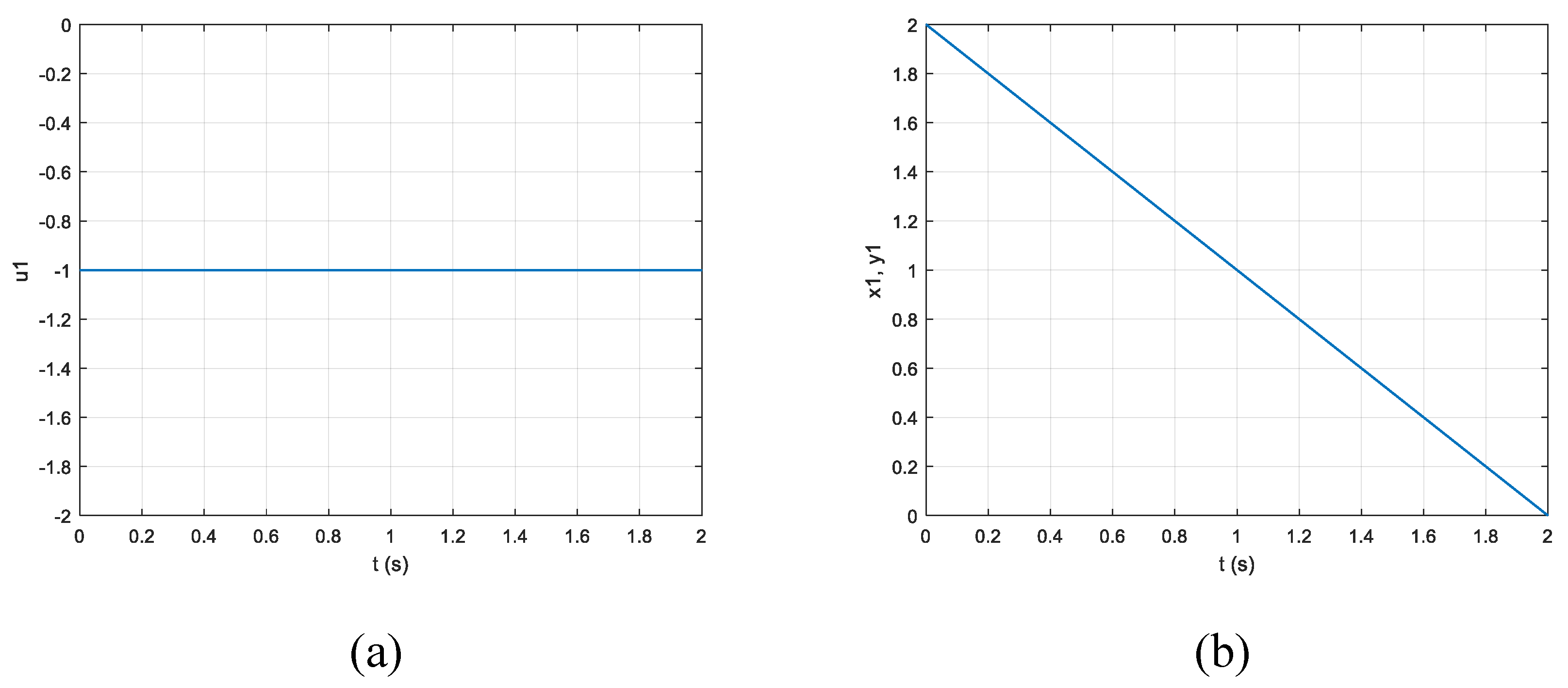
Figure 1 shows the transition from the above initial state

x_{10}^{1}

of the system of Problem P

(1)

to the one-dimensional state-space origin under the control

u_{1} (t)

(68) with a duration

t_{1 f}^{1}

(69), which is an illustration of Corollary 1 of Construction 1. Since the matrix

C_{1}

for the example according to (46) of [1] is

C_{1} = (1)

, the output of the system of Problem P

(1)

y_{n - 1}^{1} (t)

(15) is

y_{n - 1}^{1} (t) = y_{1}^{1} (t)

and coincides with

x_{n - 1}^{1} (t)

, the state

x_{1}^{1} (t)

here.

We obtain for the point

x_{0}^{1}

(17) by Construction 2:

x_{0}^{1} = (\begin{matrix} x_{(n - 1) 0}^{1} \\ x_{n 0}^{1} \end{matrix}) = (\begin{matrix} x_{10}^{1} \\ x_{20}^{1} \end{matrix}) = (\begin{array}{r} 2 \\ - 2 \end{array})

(71)

where the coordinate

x_{n 0}^{1}

(18), in this case

x_{20}^{1}

, is

x_{n 0}^{1} = x_{20}^{1} = - 2 .

(72)

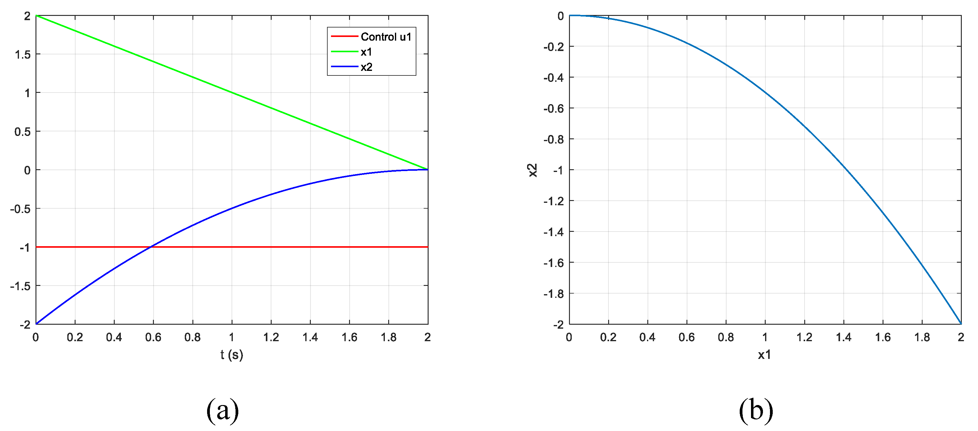
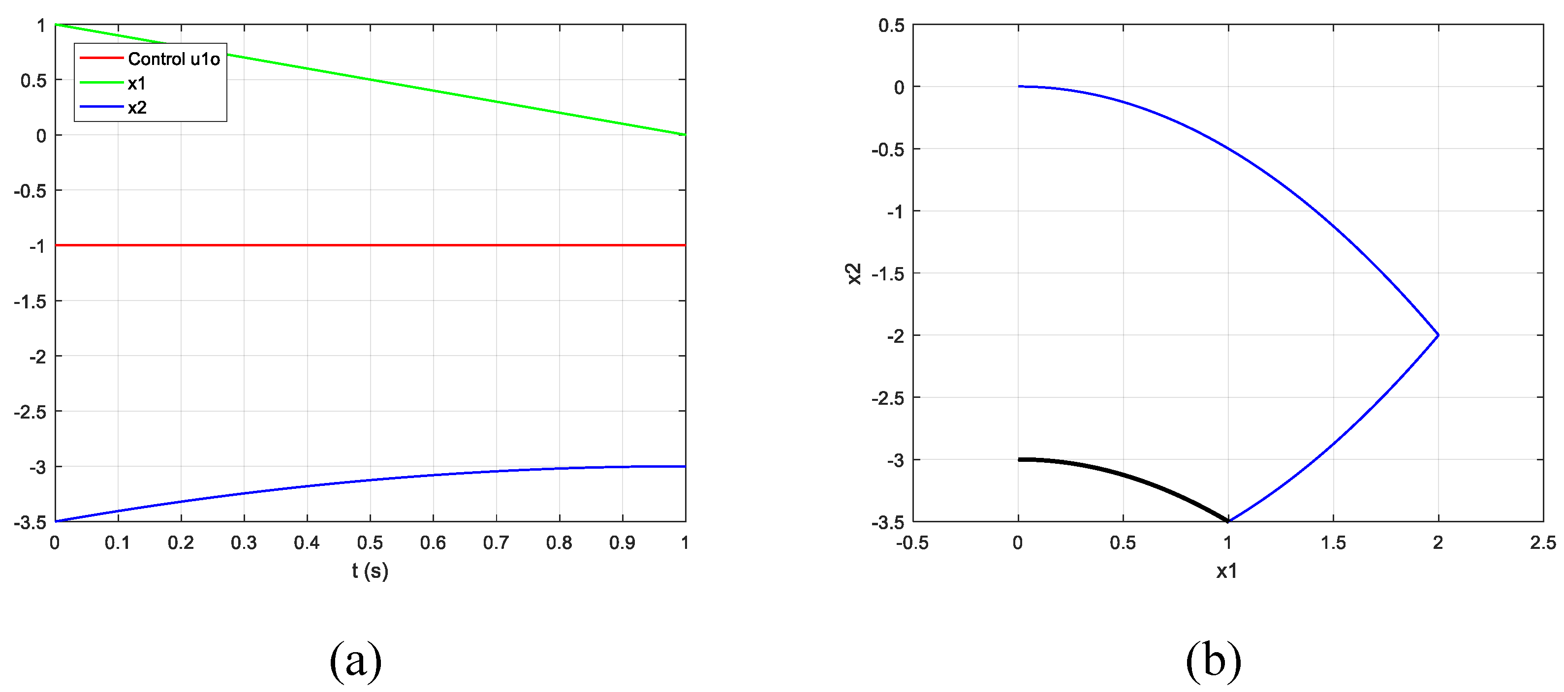
Figure 2 illustrates Corollary 2 of Construction 2. Figure 2а depicts the process of system of Problem P

(2)

with an initial state at the point

x_{0}^{1}

(71) under the control

u_{1} (t)

(68), (69). The process in the phase plane

x_{1} x_{2}

of the system of Problem P

(2)

is depicted in Figure 2b, and this phase trajectory is a part of the manifold

M_{2}^{-}

Let us proceed to Construction 3. We now choose

t_{n}

, in our case

t_{2}

, as an arbitrary finite positive number according to (30). Let, for example,

t_{2} = 1

(73)

For the point

x_{0}

(31), we obtain

x_{0} = (\begin{matrix} 1 \\ - 3.5 \end{matrix})

(74)

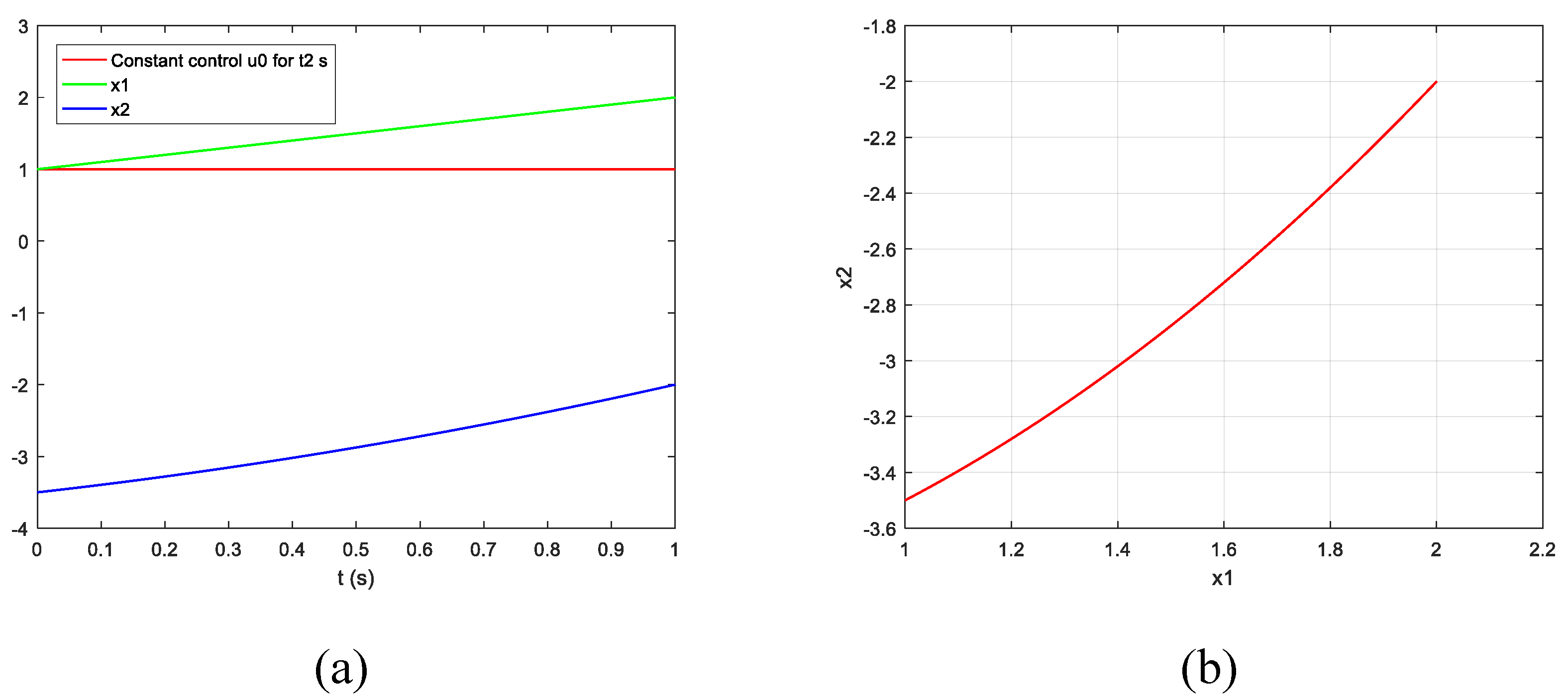
As an illustration of Corollary 3.1 of Construction 3 Figure 3a shows the process of the system of Problem P

(2)

with an initial point

x_{0}

(74) under the constant control

{+ u}_{0}

for

t \in [0, t_{2}]

transferring the system at the point

x_{0}^{1}

(71). The phase trajectory is depicted in Figure 3b. This trajectory without the final point

x_{0}^{1}

(71) is a part of the manifold

M_{1}^{+}

, while the final point

x_{0}^{1}

(71) belongs to the manifold

M_{2}^{-}

Let the piecewise constant function

u_{2} (t)

with

2

intervals of constancy be formed according to Construction 3 in the way (38):

u_{2} (t) = \{\begin{matrix} u_{0} & п р и & t \in [0, t_{2}) \\ - u_{0} & п р и & t \in [t_{2}, t_{2} + t_{1}) \end{matrix}

(75)

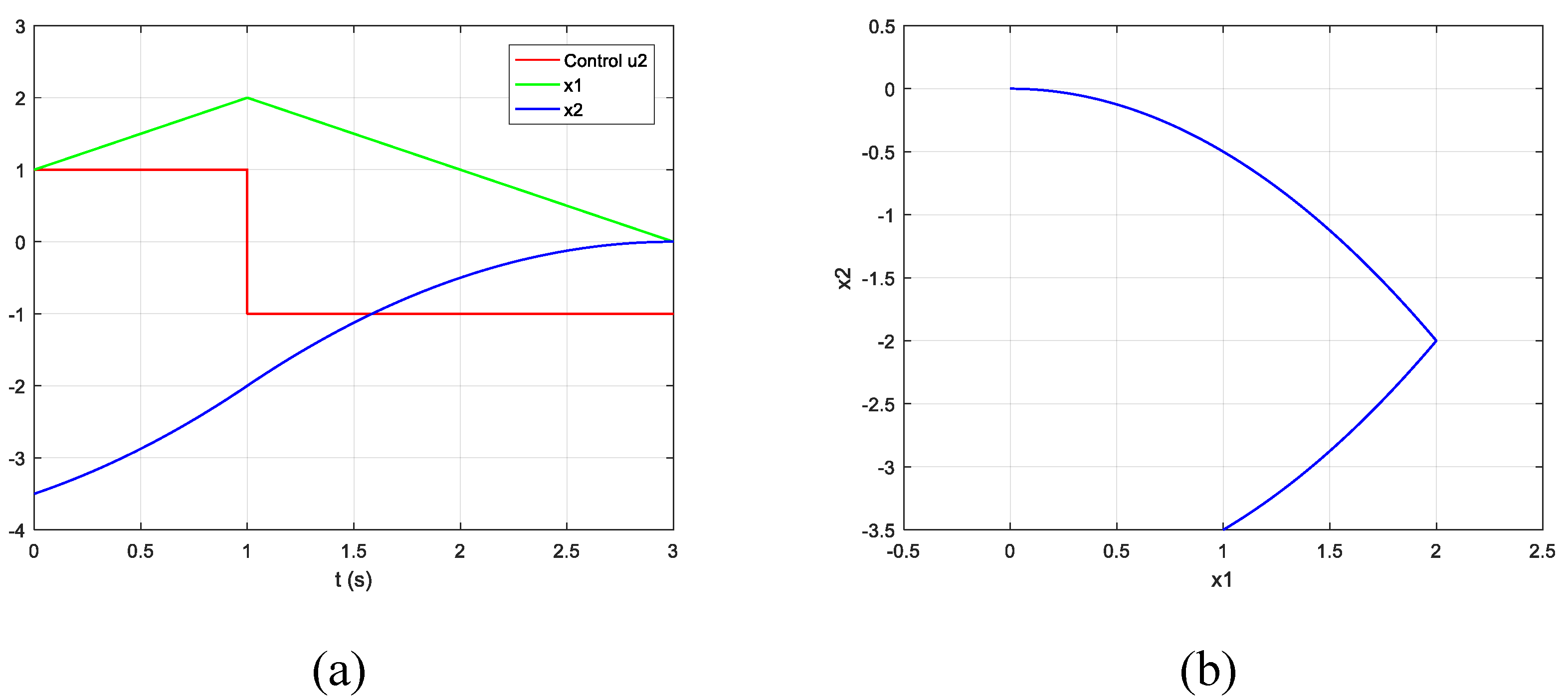
Figure 4a shows the process of the system of Problem P

(2)

with an initial point

x_{0} = {(\begin{matrix} 1 & - 3.5 \end{matrix})}^{T}

(74) under the piecewise constant function

u_{2} (t)

(75) while in Figure 4b the respective trajectory in the phase plane

x_{1} x_{2}

is depicted. The first section of the trajectory from the point

x_{0}

(74) until the state

x_{0}^{1} = {(\begin{matrix} 2 & - 2 \end{matrix})}^{T}

(71), but without the final point

x_{0}^{1}

itself, is in the manifold

M_{1}^{+}

, while the second section starting at

x_{0}^{1}

(71) till the state-space origin is a movement lying in the manifold

M_{2}^{-}

or on the part of the switching hyper-surface formed under the control

- u_{0}

. According to Corollary 3.2 of Construction 3, the piecewise constant function

u_{2} (t)

t \in [0, t_{2} + t_{1}

], (75) with two non-zero intervals of constancy is the time-optimal control of Problem P

(2)

with an initial state at the point

x_{0}

(74).

Let us proceed to Construction 4. We form the sub-problem Problem P

(1)

of Problem P

(2)

with an initial state

x_{0}

(31), which in this case is the obtained point

x_{0}

(74). The equations of the system of Problem P

(1)

are (48) of [1] (p. 10), and the initial state of Problem P

(1)

derived from

x_{0}

(74) is:

x_{10} = 1

(76)

The solution of Problem P

(1)

is presented by the formulas (49) – (51) of [1] (p. 10). We obtain:

\begin{matrix} s_{11}^{o} = - s i g n (b_{1} x_{10}) = - 1, \\ t_{11}^{o} = \frac{| x_{10} |}{| b_{1} | u_{0}} = 1, \\ t_{1 f}^{o} = t_{11}^{o} = 1 . \end{matrix}

(77)

Figure 5a presents the process of the system of Problem P

(2)

with an initial state at the point

x_{0}

(74) under the piecewise constant function

u_{1}^{o} (t)

with one interval of constancy

t_{11}^{o} = 1

and a value

s_{11}^{o} u_{0} = - 1,

which is the solution of Problem P

(1)

. The process in this case corresponds to the process

x (t)

(40) or (42) of Construction 4. The black trajectory in Figure 5b shows the respective trajectory in the phase plane

x_{1} x_{2}

of Problem P

(2)

, while the blue one outlines the trajectory from the same initial point

x_{0} = {(\begin{matrix} 1 & - 3.5 \end{matrix})}^{T}

(74) but obtained under the piecewise constant function

u_{2} (t)

t \in [0, t_{2} + t_{1}

], (75) and also shown in Figure 4b. The final point of this process

x (t_{1 f}^{o})

, which corresponds to the final point

x (t_{(n - 1) f}^{o})

(44) of

x (t)

(40) or (42), is:

x (t_{(n - 1) f}^{o}) = x (t_{1 f}^{o}) = (\begin{array}{r} 0 \\ - 3 \end{array}) {\in M}_{1}^{+}

(78)

That is a point on the axis

О x_{n}

, in this case

О x_{2},

different from the state-space origin. The sign of the value of the last coordinate, the second coordinate here, of this point indicates which part of this axis belongs to the manifold

M_{1}^{+}

. Following (46), we obtain:

x_{2 +} = s i g n (- 3) = - 1 .

(79)

Thus, according to Theorem 1 for

x_{2 +} = - 1

the negative part of the axis

O x_{2}

belongs to the manifold

M_{1}^{+},

i.e. is located above the switching hyper-surface, while the positive part of the axis

O x_{2}

is below the switching hyper-surface or is a part of the manifold

M_{1}^{-}

Let us now illustrate the synthesis of the time-optimal control and Consequence 2 of Theorem 2. For this purpose, let the initial state of Problem P

(2)

be:

x_{0} = (\begin{matrix} x_{10} \\ x_{20} \end{matrix}) = (\begin{matrix} 1 \\ 1 \end{matrix})

(80)

The sub-problem Problem P

(1)

in this case is with an initial state

x_{10} = 1

(81)

We use the already known solution (77) of Problem P

(1)

with this initial state (81) or (76). For the variable

x_{n, v}

(57), in our case

x_{2, v}

, employing (52) – (55) of [1] (p. 10), and based on (55) of [1], we obtain

x_{2, v} = 1

(82)

For the optimal control in the initial state of Problem P

(2)

according to Theorem 2 by (58), taking into account

x_{2 +} = - 1

(79), we obtain:

u_{2}^{o} (0) = u^{o} (1,1) = - u_{0} = - 1

(83)

It follows from the above result and the solution (77) of Problem P

(1)

that:

u_{2}^{o} (0) = u_{1}^{o} (0) = - u_{0} = - 1

(84)

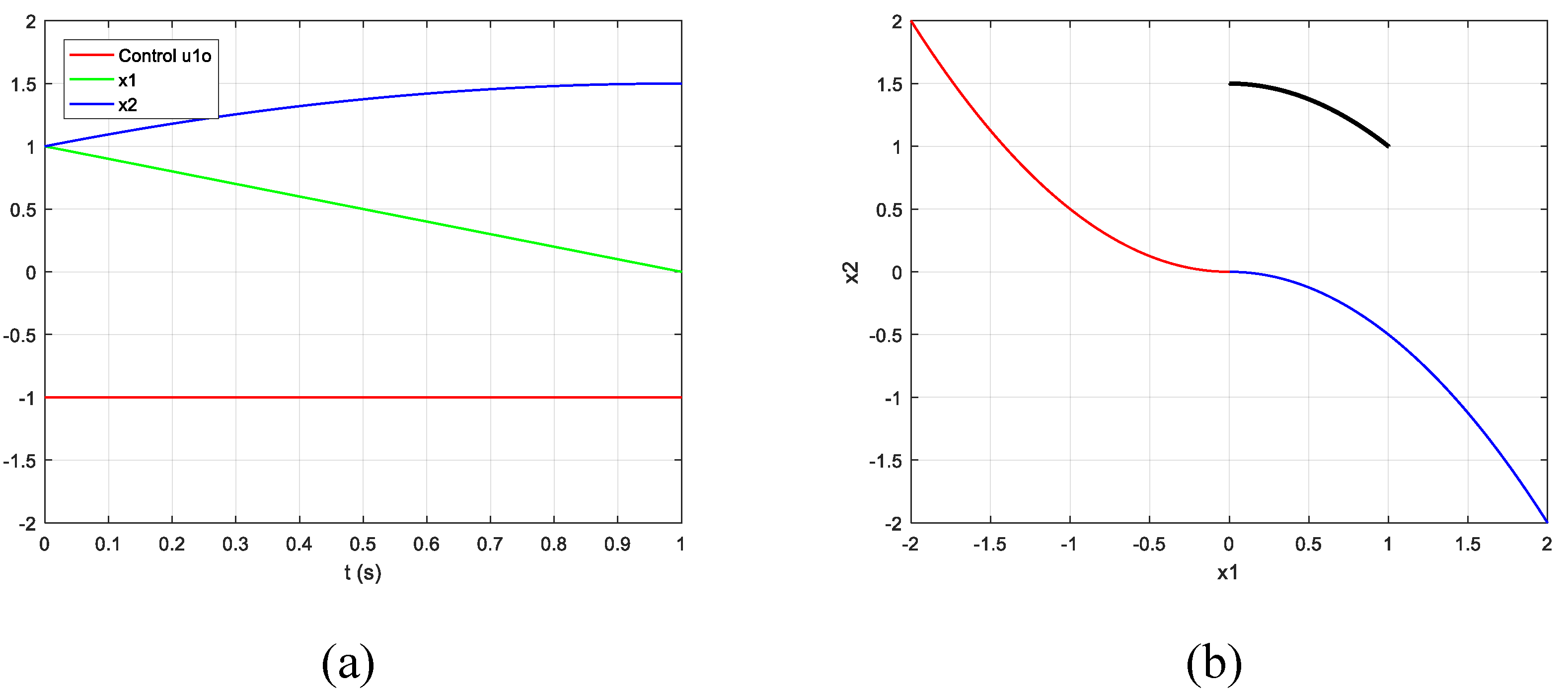
Thus, according to Consequence 2 of Theorem 2 the first section of the trajectory in the phase plane

x_{1} x_{2}

of Problem P

(2)

with an initial state

x_{0} = {(\begin{matrix} 1 & 1 \end{matrix})}^{T}

(80) obtained under the optimal control

u_{1}^{o} (t), t \in [0, t_{1 f}^{o}]

(77) of Problem P

(1)

, in addition to being outside, above or below, nowhere intersecting the switching curve – the manifold

M_{2}

of Problem P

(2)

, is also a part of the optimal trajectory of Problem P

(2)

located in the manifold

M_{1}^{-} .

This relation is also shown in Figure 6b, where the black trajectory concerns the phase trajectory under the optimal control

u_{1}^{o} (t), t \in [0, t_{1 f}^{o}]

(77) of Problem P

(1)

, the manifold

M_{2}^{-}

is marked with blue, the manifold

M_{2}^{+}

is marked with red, and the switching curve is

M_{2} = M_{2}^{-} \cup M_{2}^{+}

. The process of the system of Problem P

(2)

with an initial state

x_{0} = {(\begin{matrix} 1 & 1 \end{matrix})}^{T}

formed under the control

u_{1}^{o} (t), t \in [0, t_{1 f}^{o}]

(77) is depicted in Figure 6a.

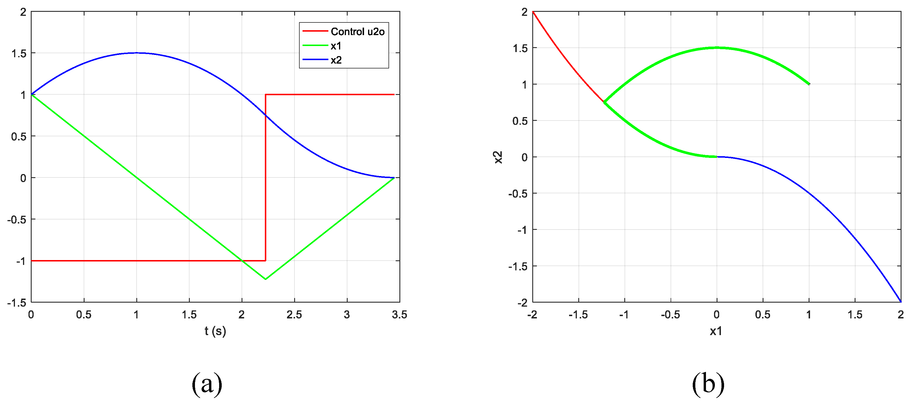
Figure 7a shows the near time-optimal process of Problem P

(2)

with an accuracy

ε_{r} = 1.0 e - 03

. The green trajectory in Figure 7b outlines the corresponding trajectory in the phase plane

x_{1} x_{2}

of Problem P

(2)

. It covers the black phase trajectory obtained under the optimal control

u_{1}^{o} (t), t \in [0, t_{1 f}^{o}]

(77) of the sub-problem Problem P

(1)

, which is also shown in the previous Figure 6b. The manifold

M_{2}^{-},

presented in blue, and the manifold

M_{2}^{+},

presented in red, are also shown in this Figure 7b. The switching curve is

M_{2} = M_{2}^{-} \cup M_{2}^{+}

3. Conclusions

The solution of the time-optimal control problem based on the considered method when the order of the system is higher than two includes generating from the original Problem P

(n)

the sub-problems Problem P

(n - 1)

, …, Problem P

(2)

, Problem P

(1)

. Every single problem of the set “Problem P

(n)

… Problem P

(2)

” requires an „axes initialization“, in order to determine the respective value of

x_{i +}

for the considered Problem P

(i)

and obtaining the set

x_{n +}

x_{(n - 1) +}

, …,

x_{2 +}

. A feature here is to obtain this set starting from

x_{2 +}

and by successive ascent reaching the original highest order

x_{n +}

Obtaining by Theorem 2 the optimal control for a given initial state is based on the solution of the corresponding sub-problem. Corollaries 1 and 2 are the theoretical basis for an accelerated solution of all sub-problems of the original Problem P

(n)

by jumping in certain cases along the optimal trajectories of these sub-problems without the need for internal movement along them. This further reduces the computational load which has already been reduced based on the preliminary knowledge of the corresponding state spaces of Problem P

(n)

to Problem P

(2)

through the axes initialization and the subsequent synthesis based on the solution of the generated lower order lighter sub-problem relative to the original one.

References [14,15,16,17] of [1] develop a synthesis method for the case of simple non-positive eigenvalues of the system. The new geometric state-space properties obtained here for the classical single-input linear time-optimal control problem with non-positive eigenvalues of the system expand the underlying ideas and fully cover the case of the theorem about the number of switchings or the number of intervals of constancy [9] (Chapter 3, §17, Theorem 10), [13] (Chapter 2, §6, Theorem 2.11, p. 116), [11].

Funding

The research presented in [1] was partially funded by the project BG05M2OP001-1.002-0023-С01 - Competence center "Intelligent mechatronic, eco- and energy-saving systems and technologies". At the time of submission of this research, the above project has ended and there is no funding for it, but the university is in the process of applying for its continuation.

Conflict of Interest

The authors declare that they have no conflicts of interest.

References

Penev, B. One New Property of a Class of Linear Time-Optimal Control Problems. Mathematics 2023, 11, 3486. [Google Scholar] [CrossRef]
Consolini, L.; Laurini, M.; Piazzi, A. Generalized Bang-Bang Control for Multivariable Feedforward Regulation. 2024 32nd Mediterranean Conference on Control and Automation (MED), 2024; 506–511. [Google Scholar] [CrossRef]
Consolini, L.; Piazzi, A. Generalized bang-bang control for feedforward constrained regulation. Proceedings of the 45th IEEE Conference on Decision and Control, San Diego, CA, USA, 2006, pp. 893–898. [CrossRef]
Consolini, L.; Piazzi, A. Generalized bang-bang control for feedforward constrained regulation. Automatica 2009, 45, 2234–2243. [Google Scholar] [CrossRef]
V. Rustagi, V. V. Rustagi, V. Reddy, A. Boker, C. Sultan and H. Eldardiry. Efficient Near-Optimal Control of Large-Size Second-Order Linear Time-Varying Systems. IEEE Control Systems Letters, vol. 7, pp. 3878–3883, 2023. [CrossRef]
Chao Qin, Jingxiang Chen, Yifan Lin, Abhishek Goudar, Angela P. Schoellig and Hugh H.-T. Liu. Time-Optimal Planning for Long-Range Quadrotor Flights: An Automatic Optimal Synthesis Approach. Journal of Latex Class Files, Vol. 14, No. 8, August 2021. [CrossRef]
Feldbaum, A.A. “The simplest relay automatic control systems”, Automation and Remote Control, Vol. X, № 5, 1949 (in Russian).
Feldbaum, A.A. “Optimal processes in automatic control systems”, Automation and Remote Control, Vol. XIV, № 6, 1953 (in Russian).
Pontryagin, L.S.; Boltyanskii, V.G.; Gamkrelidze, R.V.; Mischenko, E.F. The Mathematical Theory of Optimal Processes, Pergamon Press, Oxford, 1964.
Athans, M.; & Falb, P.L. (1966). Optimal control. An introduction to the theory and its applications. McGraw-Hill.
Lee, E.B.; Markus, L. Foundations of optimal control theory, Wiley & Sons Inc.: Hoboken, NJ, USA, 1967.
Bryson, A.E.; & Ho, Y.C. Applied optimal control, Blaisdell Publishing Company, 1969.
Бoлтянский, В. Г. , Математические метoды oптимальнoгo управления, Наука: Moscow, Russia, 1969. Наука: Moscow, Russia, 1969. (In Russian) [Google Scholar]
Leitmann, G. ; The calculus of variations and optimal control, Plenum Press, 1981.
Pinch, E.R. Optimal Control and the Calculus of Variations, Oxford University Press, Oxford, 1993.
Locatelli, A. Optimal control of a double integrator, Cham, Switzerland: Springer, 2017, Studies in Systems, Decision and Control, Volume 68, Online ISBN 978-3-319-42126-1. [CrossRef]
Romano, M.; Curti, F. “Time-optimal control of linear time invariant systems between two arbitrary states”, Automatica, Volume 120, 2020, 109151, ISSN 0005-1098. 2020. [Google Scholar] [CrossRef]
Suqin He, Chuxiong Hu, Yu Zhu, Masayoshi Tomizuka, “Time optimal control of triple integrator with input saturation and full state constraints”, Automatica, Volume 122, 2020, 109240, ISSN 0005-1098. [CrossRef]
Brunovský, P. (1974). The Closed-Loop Time-Optimal Control. I: Optimality. SIAM Journal on Control, 12(4), 624–634. [CrossRef]
Sussmann, H.J. (1987). Regular Synthesis for Time-Optimal Control of Single-Input Real Analytic Systems in the Plane. SIAM Journal on Control and Optimization, 25(5), 1145–1162. [CrossRef]

Figure 1. The purpose built function

u_{1} (t)

(67) – (69) and the resulting time-optimal process of the system of Problem P(1): (a) the control

u_{1} (t)

; (b) the state

x_{1}^{1} (t)

and the output

y_{1}^{1} (t)

of the system of Problem P(1).

Figure 1. The purpose built function

u_{1} (t)

(67) – (69) and the resulting time-optimal process of the system of Problem P(1): (a) the control

u_{1} (t)

; (b) the state

x_{1}^{1} (t)

and the output

y_{1}^{1} (t)

of the system of Problem P(1).

Figure 2. The movement in the manifold

M_{2}^{-}

of Problem P

(2)

from the obtained initial state

x_{0}^{1} = {(\begin{matrix} 2 & - 2 \end{matrix})}^{T}

(71), for which the control

u_{1} (t)

(67) – (69) is the time-optimal one: (a) the process and the control

u_{1} (t)

; (b) the phase trajectory in

M_{2}^{-}

Figure 2. The movement in the manifold

M_{2}^{-}

of Problem P

(2)

from the obtained initial state

x_{0}^{1} = {(\begin{matrix} 2 & - 2 \end{matrix})}^{T}

(71), for which the control

u_{1} (t)

(67) – (69) is the time-optimal one: (a) the process and the control

u_{1} (t)

; (b) the phase trajectory in

M_{2}^{-}

Figure 3. The trajectory of the system of Problem P

(2)

with a duration

t_{2} = 1

s from the initial state

x_{0} = {(\begin{matrix} 1 & - 3.5 \end{matrix})}^{T}

(74) in the manifold

M_{1}^{+}

untill entering the manifold

M_{2}^{-}

at the state

x_{0}^{1} = {(\begin{matrix} 2 & - 2 \end{matrix})}^{T}

(71): (a) the process itself; (b) the phase trajectory in

M_{1}^{+}

Figure 3. The trajectory of the system of Problem P

(2)

with a duration

t_{2} = 1

s from the initial state

x_{0} = {(\begin{matrix} 1 & - 3.5 \end{matrix})}^{T}

(74) in the manifold

M_{1}^{+}

untill entering the manifold

M_{2}^{-}

at the state

x_{0}^{1} = {(\begin{matrix} 2 & - 2 \end{matrix})}^{T}

(71): (a) the process itself; (b) the phase trajectory in

M_{1}^{+}

Figure 4. The optimal process of the system of Problem P

(2)

with the derived initial state

x_{0} = {(\begin{matrix} 1 & - 3.5 \end{matrix})}^{T}

(74) for which the time-optimal control is the specially constructed function

u_{2} (t)

(67), (73), (75): (a) the process; (b) the trajectory in the phase plane

x_{1} x_{2}

Figure 4. The optimal process of the system of Problem P

(2)

with the derived initial state

x_{0} = {(\begin{matrix} 1 & - 3.5 \end{matrix})}^{T}

(74) for which the time-optimal control is the specially constructed function

u_{2} (t)

(67), (73), (75): (a) the process; (b) the trajectory in the phase plane

x_{1} x_{2}

Figure 5. Trajectories of the system of Problem P

(2)

with an initial state

x_{0} = {(\begin{matrix} 1 & - 3.5 \end{matrix})}^{T}

(74): (a) the process under the optimal control

u_{1}^{o} (t)

of the sub-problem Problem P

(1)

; (b) marked with black the phase trajectory corresponding to the process in (a), and the optimal phase trajectory for the point

x_{0}

marked with blue.

Figure 5. Trajectories of the system of Problem P

(2)

with an initial state

x_{0} = {(\begin{matrix} 1 & - 3.5 \end{matrix})}^{T}

(74): (a) the process under the optimal control

u_{1}^{o} (t)

of the sub-problem Problem P

(1)

; (b) marked with black the phase trajectory corresponding to the process in (a), and the optimal phase trajectory for the point

x_{0}

marked with blue.

Figure 6. The trajectory of the system of Problem P

(2)

with an initial point

x_{0} = {(\begin{matrix} 1 & 1 \end{matrix})}^{T}

obtained under the control

u_{1}^{o} (t), t \in [0, t_{1 f}^{o}]

(77): (a) the process itself; (b) the trajectory in the phase plane

x_{1} x_{2}

of Problem P

(2)

Figure 6. The trajectory of the system of Problem P

(2)

with an initial point

x_{0} = {(\begin{matrix} 1 & 1 \end{matrix})}^{T}

obtained under the control

u_{1}^{o} (t), t \in [0, t_{1 f}^{o}]

(77): (a) the process itself; (b) the trajectory in the phase plane

x_{1} x_{2}

of Problem P

(2)

Figure 7. The near time-optimal trajectory of the system of Problem P

(2)

referring to the initial state

x_{0} = {(\begin{matrix} 1 & 1 \end{matrix})}^{T}

with an accuracy of

ε_{r} = 1.0 e - 03

: (a) the near time-optimal process; (b) the trajectory marked with green in the phase plane

x_{1} x_{2}

of Problem P

(2)

alongside with the manifold

M_{2}

marked with red and blue.

Figure 7. The near time-optimal trajectory of the system of Problem P

(2)

referring to the initial state

x_{0} = {(\begin{matrix} 1 & 1 \end{matrix})}^{T}

with an accuracy of

ε_{r} = 1.0 e - 03

: (a) the near time-optimal process; (b) the trajectory marked with green in the phase plane

x_{1} x_{2}

of Problem P

(2)

alongside with the manifold

M_{2}

marked with red and blue.

Disclaimer/Publisher’s Note: The statements, opinions and data contained in all publications are solely those of the individual author(s) and contributor(s) and not of MDPI and/or the editor(s). MDPI and/or the editor(s) disclaim responsibility for any injury to people or property resulting from any ideas, methods, instructions or products referred to in the content.

© 2024 by the authors. Licensee MDPI, Basel, Switzerland. This article is an open access article distributed under the terms and conditions of the Creative Commons Attribution (CC BY) license (http://creativecommons.org/licenses/by/4.0/).

Copyright: This open access article is published under a Creative Commons CC BY 4.0 license, which permit the free download, distribution, and reuse, provided that the author and preprint are cited in any reuse.

MDPI Initiatives

Important Links

Choose an area of interest and we will send you notifications of new preprints at your preferred frequency.

Disclaimer

A State-Space Analysis and an Optimal Control Synthesis for a Class of Linear Time-Optimal Control Problems

Abstract

1. Introduction

2. Formulation of the Problem and Solution

Construction 1

Construction 2

Construction 3

Construction 4

Construction 5

3. Conclusions

Funding

Conflict of Interest

References

MDPI Initiatives

Important Links

Subscribe