Preprint
Article

A Three-Phase Novel Angular Perturbation Technique for Metaheuristic-Based School Bus Routing Optimization

Altmetrics

Downloads

385

Views

702

Comments

0

This version is not peer-reviewed

Submitted:

17 September 2024

Posted:

19 September 2024

You are already at the latest version

Alerts
Abstract
This article introduces a novel three-phase angular perturbation technique for solving the School Bus Problem (SBP), an NP-hard combinatorial optimization challenge. The three phases—initial solution, global and local search, and solution exploration—focus on optimizing school bus routes by minimizing sharp turns and reducing travel distances. The performance of three metaheuristic algorithms (GAACOSA-AP, BFSPSO-AP, RL-AP) is evaluated, and significant improvements in routing efficiency are observed. we evaluated the performance of our hybrid algorithm against the industry-leading optimization software, CPLEX, and other optimization techniques across multiple school scenarios. The results show that the GAACOSA-AP algorithm consistently outperforms its counterparts, achieving substantial reductions in travel distances, particularly for complex routes with numerous stops. The integration of Angular Perturbation was key to improving route geometry by, reducing sharp turns, and enhancing overall path optimization by an average reduction of 27.12% compared to 22.37% without Angular Perturbation.
Keywords: 
Subject: Computer Science and Mathematics  -   Mathematics

1. Introduction

The School Bus Problem (SBP) is a complex combinatorial optimization problem that focuses on designing efficient routes for school buses to transport students between their homes and school [1]. The primary objective is to minimize factors such as total travel distance or time while meeting key constraints [2]. The SBP is essential to reduce fuel costs, minimize travel time, and ensure safe and efficient transportation for students [3]. As schools face increasing budget constraints, optimizing bus routes becomes increasingly important [4]. The SBP is classified as an NP-Hard problem [5], which implies that finding an optimal solution in polynomial time is unlikely. In addition, complexity increases exponentially with the number of students and bus stops [6].
The SBP shares similarities with other hard NP problems [7], such as the Vehicle Routing Problem (VRP) and the Traveling Salesman Problem (TSP) [8,9,10]. Both VRP and TSP present routing challenges that involve capacity and time constraints, making SBP computationally difficult. The number of potential route combinations increases rapidly as the size of the problem increases. Furthermore, the task of ensuring that no bus exceeds its capacity or that students are not kept on the bus for excessive amounts of time makes finding an optimal solution even more challenging [11]. This results in the problem becoming intractable for large instances, pushing researchers to rely on heuristics and approximation methods for near-optimal solutions [12].
Researchers have applied two main categories of approaches to address the computational challenges of the SBP: exact algorithms and heuristic or approximation methods [13,14,15,16,17]. Exact algorithms aim to find optimal solutions, but they are typically computationally expensive and impractical for large-scale problems because of the combinatorial explosion. These methods include Integer Linear Programming (ILP), where the SBP is formulated as a set of linear constraints with integer variables representing routes and student assignments [18]. Although ILP solvers theoretically provide optimal solutions, they struggle with the exponential growth of possibilities as the size of the problem increases [19]. Other sophisticated techniques such as branch-and-bound and branch-and-cut have been employed to reduce computational effort by systematically exploring the solution space while pruning suboptimal branches [20]. However, even with these advanced methods, exact algorithms often become inefficient for larger instances, necessitating the exploration of heuristic and approximation methods [21].
In light of the limitations of exact methods, much of the research on SBP has concentrated on heuristic and approximation algorithms that yield feasible solutions within a reasonable time frame, albeit without guarantees of optimality [22]. Greedy algorithms [23], where buses are assigned to students step by step based on locally optimal decisions (such as assigning the nearest student to the current bus route), have been a common approach. However, these methods may perform well for small instances, but often lead to suboptimal solutions in more complex scenarios [24]. Metaheuristic algorithms such as Genetic Algorithms (GA) [25], Simulated Annealing (SA) [26], and Tabu Search [27], have proven to be effective for larger SBP instances GA [28], inspired by evolutionary processes, generates a population of potential solutions, iterating through selection, crossover, and mutation to explore a wide range of possible routes. Simulated annealing mimics the metal cooling process, allowing the algorithm to escape local optima by accepting worse solutions early in the search. Tabu Search utilizes memory structures to avoid revisiting suboptimal solutions, steering the search toward better areas of the solution space [29].
Cluster-first [30], route-second heuristics [31], another popular method, group students into clusters based on geographical proximity before determining the optimal route within each cluster. This divide-and-conquer approach simplifies the problem, allowing for more efficient handling of large datasets [32]. Hybrid algorithms that combine various methods have also been explored to leverage the strengths of multiple techniques [33]. For example, clustering combined with metaheuristics or greedy algorithms can strike a balance between solution quality and computational efficiency. With advances in computational power and machine learning, data-driven approaches are emerging. These methods use historical data on student distribution and traffic conditions to improve route optimization. Although still in their infancy, these approaches have the potential to enhance heuristic methods by providing smarter initialization points or guiding the search toward more promising areas of the solution space [34].
This study introduces a A Three-Phase angular perturbation technique [35], which integrates three stages: Initial Solution, Global and Local Search, and Solution Exploration, to optimize school bus routes systematically [36]. In essence, the first phase ensures a valid initial solution, the second phase focuses on finding an optimal route through global and local searches, and the final phase uses our novel technqie called angular perturbation to minimize sharp turns, making bus travel smoother and more efficient. Angualar pertubation is an optimization technique that has been inispired and slightly similar but different to the works from [38,39,40,41,42]. These researchers used different state of the art optimization techniques that led to their near-optimal solution.
The initial solution phase generates a basic and feasible route, often using algorithms like Breadth-First Search (BFS). This solution serves as a starting point for further optimization, but may not be optimal in terms of travel distance or time. Next, the global and local search explores different route configurations, ensuring that the algorithm does not get stuck in a local minimum [43]. The global search reorders the bus stops to find a near-optimal solution, while the local search fine-tunes the current route. Finally, the solution exploration stage employs the Angular Perturbation Technique to refine the solution by minimizing sharp turns, thus smoothing the route and reducing the travel distance.
We propose three metaheuristic approaches for school bus routing: GAACOSA, BFS-PSO, and Reinforcement Learning (RL), each utilizing angular perturbation to improve route efficiency. In the GAACOSA-AP approach, GA generates an initial population of feasible routes, ACO explores the best routes globally by reinforcing efficient paths, and SA refines the best solutions locally by accepting worse solutions to escape local optima. Finally, angular perturbation adjusts sharp turns to ensure geometric optimization.
In the BFSPSO-AP method, BFS guarantees a feasible initial solution by visiting each bus stop once. PSO then improves this solution by exploring various sequences of stops to minimize the travel distance. Angular perturbation further refines the route by smoothing sharp turns. Similarly, the RL-AP approach uses a reinforcement learning agent to learn the best policy to select the next bus stop, with an angular perturbation applied afterward to improve the geometry and efficiency of the route. The key contributions of this paper are as follows:
  • We introduce The Three-Phase Novel Angular Perturbation Technique for school bus routing, which integrates three key phases: Initial Solution, Global and Local Search, and Solution Exploration.
  • A novel angular perturbation technique is employed to minimize sharp turns, optimizing route efficiency by focusing on the geometric aspects of the school bus routes.
  • We propose three metaheuristic algorithms: GAACOSA-AP, BFSPSO-AP, and RL-AP, each incorporating angular perturbation to enhance route optimization performance.
  • The hybrid GAACOSA-AP method leverages the strengths of Genetic Algorithms, Ant Colony Optimization, and Simulated Annealing, achieving global and local route optimizations.
  • BFSPSO-AP provides a systematic exploration of bus stop sequences, improving route efficiency through Particle Swarm Optimization followed by angular perturbation refinement.
  • The RL-AP method demonstrates the application of reinforcement learning to the SBP, improving the route selection policy, and further optimizing the route geometry through angular perturbation.
The remainder of this paper is organized as follows. Section 2 introduces the formal formulation of the problem, while Section 3 provides a comprehensive overview of the proposed algorithms. Subsequently, Section 4 presents the experimental results and analysis in Section 5 . Finally, Section 6 concludes the paper with final remarks and suggestions for future research.

2. Problem Formulation

In the following, we define the variables used and formulate the problem mathematically. The decision variables are represented as X = x i j i , j 0 , 1 , , n , where each x i j indicates whether the bus travels from stop i to stop j. The objective is to minimize the total travel distance, ensuring that each stop is visited exactly once, and the bus starts and ends at the school.
The problem’s variables are summarized below:
Table 1. Variables and their Description
Symbol Description
S School (depot) location
V i Set of bus stops V = { v 1 , v 2 , , v n }
d ( i , j ) Distance between stop i and stop j
x i j Binary decision variable: 1 if the bus travels from stop i to stop j,
0 otherwise
n Total number of bus stops
D Total distance traveled by the bus
The objective is to minimize the total distance traveled by the school bus while ensuring that the route starts and ends at the school and each bus stop is visited exactly once.

Decision Variable Constraints

The bus must start from the school and return to the school after visiting all bus stops:
j = 1 n x S , j = 1 , i = 1 n x i , S = 1
This ensures that the bus begins and ends its journey at the school.

Visiting Constraints

Each bus stop must be visited exactly once:
i = 0 n x i j = 1 , j = 0 n x i j = 1 i , j V
This ensures that each stop is visited only once.

Binary Decision Variables

The decision variable x i j is binary, indicating whether the bus travels from stop i to stop j:
x i j { 0 , 1 } i , j { S , V }

Objective Function

The objective is to minimize the total travel distance D:
D = i = 0 n j = 0 n d ( i , j ) · x i j
The formulation of the function minimizes:
D = i = 0 n j = 0 n d ( i , j ) · x i j
subject to:
j = 1 n x S , j = 1 , i = 1 n x i , S = 1
i = 0 n x i j = 1 , j = 0 n x i j = 1 i , j V
and
x i j { 0 , 1 } i , j { S , V }
to find the optimal route that minimizes the total distance traveled.

3. Proposed Method

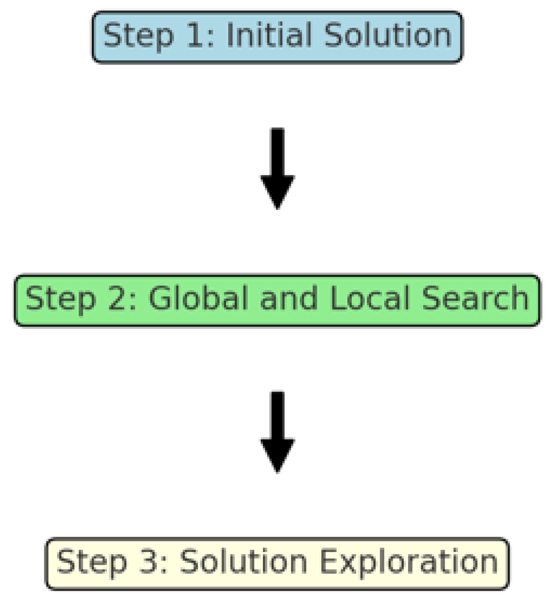
This study introduces a novel three-phase angular perturbation technique, which integrates three stages: Initial Solution, Global and Local Search, and Solution Exploration, to optimize school bus routes systematically. In essence, the first phase ensures a valid initial solution, the second phase focuses on finding an optimal route through global and local searches, and the final phase uses angular perturbation to minimize sharp turns, making bus travel smoother and more efficient.
Figure 1. A Three Phase Approach
Preprints 118492 g001
We propose three metaheuristic approaches to solve the school bus routing problem: a hybrid of Genetic Algorithm, Ant Colony Optimization, and Simulated Annealing with Angular Perturbation Technique (GAACOSA-AP), a combination of Breadth-First Search and Particle Swarm Optimization with Angular Pertubation (BFSPSO-AP), and Reinforcement Learning with Angular Pertubation (RL-AP). A key element in all three methods is the incorporation of angular perturbation, a technique that plays a pivotal role in optimizing the route. Angular perturbation is an optimization technique designed to improve the geometric structure of routes by focusing on the angles formed between consecutive stops. In a typical route, three consecutive bus stops, say v a , v b , and v c , form an angle at the middle stop v b . The goal of angular perturbation is to adjust this angle to make the transitions between stops smoother, ultimately reducing the total travel distance.
To illustrate, consider the angle θ formed at bus stop v b between the two vectors v a v b and v b v c . The angle can be computed using the cosine rule:
cos θ a b c = d a b 2 + d b c 2 d a c 2 2 d a b d b c
where d a b , d b c , and d a c represent the distances between stops v a , v b , and v c , respectively. Angular perturbation works by introducing small changes to this angle θ , exploring alternative configurations that reduce the sharpness of turns.
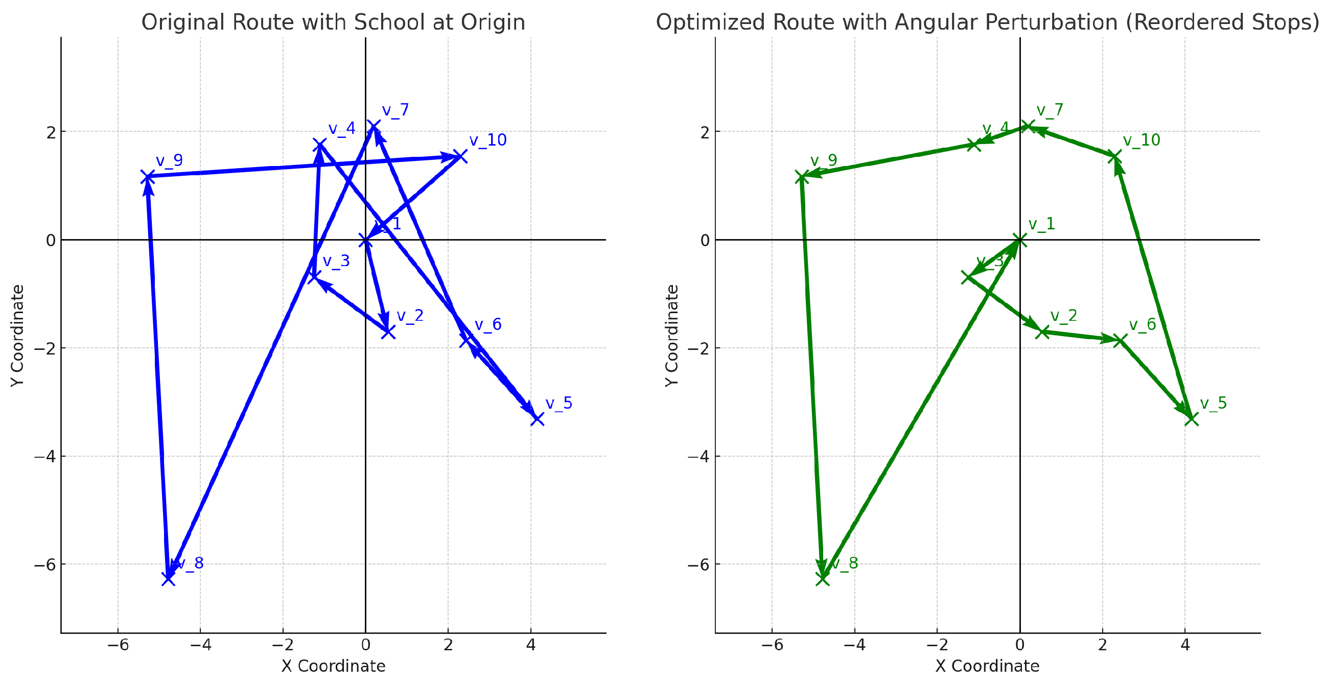
To visualize the Angular pertubation concept as demonstrated in Figure 2, we start with a route comprising 10 bus stops, Each plot represents a series of bus stops (denoted as v 1 , v 2 , , v 10 ) connected by lines to illustrate the bus route starting and ending at the school, which is placed at the origin ( 0 , 0 ) . The graph illustrates the direction of travel with arrows, showing the path from the school through all stops and back to the school. In the original route at the left side in blue, are bus stops connected in a predefined sequence. This sequence may involve sharp angles between some stops, leading to inefficient turns. while, on the right side in green the optimized route uses angular perturbation to minimize the sharpness of turns. By reordering the sequence in which the bus stops are visited, the route becomes smoother, with fewer abrupt direction changes. The comparison between the two graphs highlights the effectiveness of angular perturbation. While the bus stop locations remain the same, the optimized route achieves smoother transitions, ultimately reducing the total travel distance and time. This approach can lead to substantial benefits, such as lower fuel consumption, less wear and tear on vehicles, and improved travel experiences for passengers due to fewer abrupt turns.

3.0.1. Genetic Algorithm, Ant Colony Optimization, and Simulated Annealing with Angular Perturbation Technique (GAACOSA-AP)

In this section, we present the hybrid approach for solving the School Bus Routing Problem (SBRP), combining Genetic Algorithm (GA), Ant Colony Optimization (ACO) and Simulated Annealing (SA), along with the novel angular perturbation technique. The equations and variables are introduced as follows.
We define the set of bus stops as V = { v 0 , v 1 , , v n } , where v 0 represents the school, and each v i for i 1 represents a specific bus stop. The objective is to minimize the total distance traveled by bus while visiting all stops and returning to the school.
The fitness function for the Genetic Algorithm is expressed as follows:
Fitness ( π ) = D ( π ) = i = 0 n 1 d π ( i ) π ( i + 1 ) + d π ( n ) π ( 0 )
Here, D ( π ) is the total distance for a route π , where π ( i ) denotes the i-th stop in the sequence. The term d π ( i ) π ( i + 1 ) is the distance between consecutive stops π ( i ) and π ( i + 1 ) , and d π ( n ) π ( 0 ) represents the distance from the last stop to the school. The GA uses crossover and mutation operators to evolve the population, ensuring diversity and exploration of various route configurations.
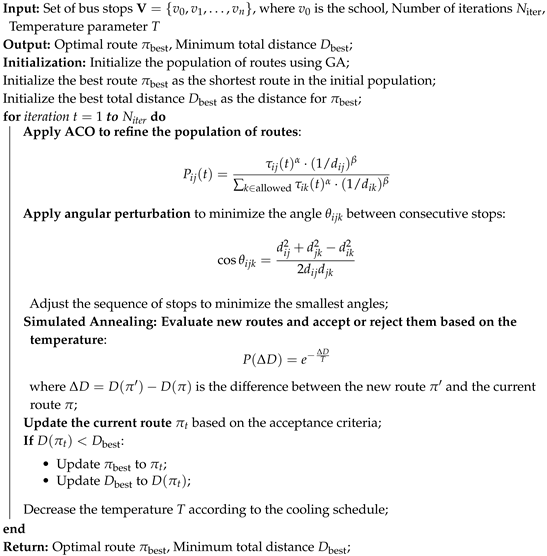
After the initial population is generated by GA, Ant Colony Optimization (ACO) is applied to refine these routes. ACO simulates the behavior of ants, where each ant builds a potential route based on pheromone trails. The pheromone matrix τ i j tracks the level of pheromones for traveling between stops v i and v j , with v i and v j representing consecutive bus stops. The probability that an ant will choose to travel from stop v i to stop v j is given by the following:
P i j ( t ) = τ i j ( t ) α · ( 1 / d i j ) β k allowed τ i k ( t ) α · ( 1 / d i k ) β
In this equation, α controls the influence of the pheromone trail, and β controls the influence of the inverse distance d i j between stops v i and v j . The denominator sums all the next allowed stops k (other possible stops). As ants traverse the routes, they deposit pheromones, reinforcing shorter and more desirable paths.
After ACO has refined the routes, the angular perturbation technique is applied to further improve the solution. For three consecutive stops v i , v j , and v k , the angle θ i j k at stop v j is calculated using the cosine rule:
cos θ i j k = d i j 2 + d j k 2 d i k 2 2 d i j d j k
where d i j , d j k , and d i k are the distances between stops v i , v j , and v k . The goal of this perturbation step is to minimize the angle θ i j k to reduce sharp turns, resulting in a more efficient route. Smaller angles generally indicate smoother transitions and reduced travel distance.
Once ACO and angular perturbation have been applied, Simulated Annealing (SA) is used to further improve the solution by escaping local optima. SA allows the system to accept worse solutions with a certain probability, helping the algorithm explore other regions of the solution space. The acceptance probability of a worse solution is defined by:
P ( Δ D ) = e Δ D T
where Δ D = D ( π ) D ( π ) is the difference in distances between the new route π and the current route π . The temperature parameter T decreases with time, reducing the probability of accepting worse solutions as the algorithm progresses. This balance between exploration and exploitation allows the algorithm to refine the current best solution while still exploring alternative routes.
In summary, this hybrid approach integrates GA for generating an initial population of routes, ACO for refining routes based on pheromone trails, angular perturbation for optimizing the geometry of the routes by minimizing sharp angles, and SA for ensuring the solution does not get trapped in local optima.
Algorithm 1: GAACOSA-AP for SBR
Preprints 118492 i001
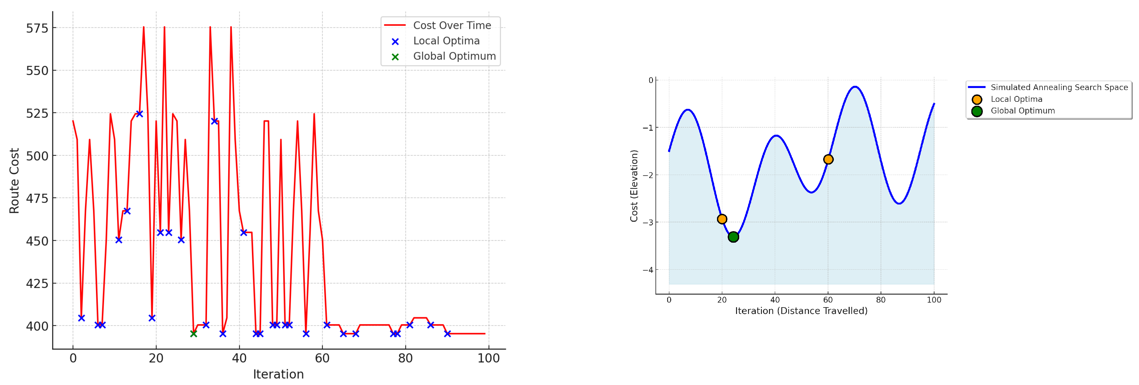
The Figure 3, demonstrates, SA’s effectiveness in navigating complex solution spaces by accepting suboptimal solutions temporarily to eventually reach the best possible outcome.

3.0.2. Breadth-First Search and Particle Swarm Optimization with Angular Pertubation (BFSPSO-AP)

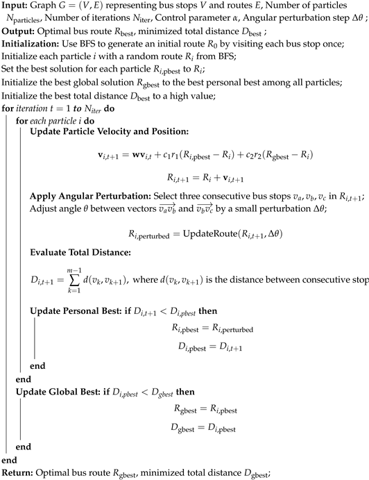
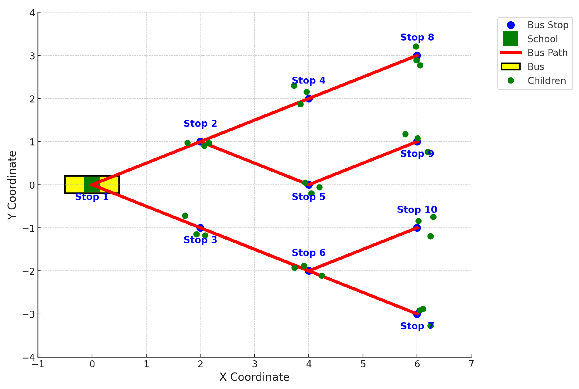
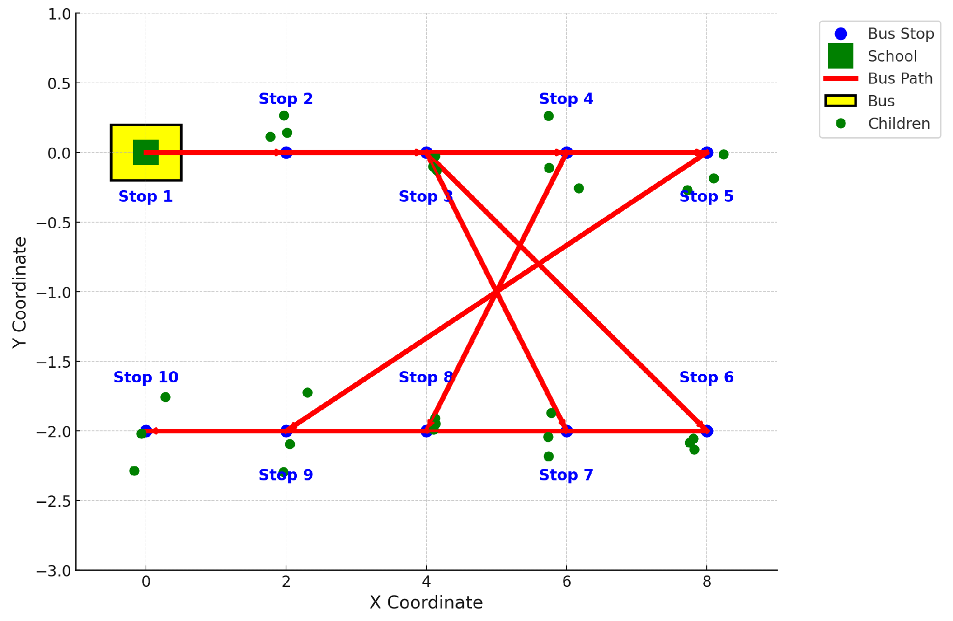
In this hybrid approach to optimizing the route of school buses, the process begins with breadth-first search (BFS) for the traversal of the route, followed by particle swarm optimization (PSO) and angular perturbation (AP) for optimizing the route. BFS starts by treating the school as the starting point, denoted as v 0 , and systematically explores the graph, where each vertex represents a bus stop and each edge represents a connection between stops. In each step, the BFS traverses an edge e i j , which is the connection between bus stops v i and v j . BFS ensures that all bus stops are visited once, providing an initial route configuration that serves as a foundation for further optimization. The graphs in Figure 4 and Figure 5, illustrate the BFS traversal for a school bus visiting 10 bus stops. The bus at Figure 4, starts at Stop 1, represented by the green square, and follows the red edges, visiting nearby stops in sequence. The numbers next to each stop indicate the order in which the bus visits each location to pick up children. In the first diagram, the bus starts its route at Stop 1 and moves to Stops 2 and 3, which are the closest neighbors to the starting point. From Stop 2, the bus proceeds to Stops 4 and 5, while from Stop 3, it continues to Stops 6 and 7. The bus then completes its journey by visiting Stops 8, 9, and 10 before returning to Stop 1, thus demonstrating a structured and efficient path with minimal intersections.
In Figure 5, follows the same traversal from Stop 1 to Stop 10, but in this case, the route is more complex with multiple path intersections, suggesting a less optimized approach compared to the first figure. These diagrams demonstrate how BFS works by visiting adjacent stops first before moving further away, presenting two different scenarios for completing the bus route efficiently.
Once BFS generates the initial traversal, PSO is used to optimize the route. In PSO, each potential solution is represented as a particle, with a set of particles P = { p 1 , p 2 , , p n } , where each particle p i represents a candidate bus route. Each particle has a position x i and a velocity v i , which define its movement through the solution space. The position x i ( t ) at a given iteration t represents the sequence in which the bus stops are visited, and the velocity v i ( t ) determines how the route is updated in subsequent iterations. The fitness function f ( p i ) measures the quality of the solution and is defined as the total distance from the road:
f ( p i ) = k = 1 m 1 d ( v k , v k + 1 ) ,
where d ( v k , v k + 1 ) is the distance between consecutive bus stops v k and v k + 1 , and m is the total number of stops. The objective is to minimize f ( p i ) , thus minimizing the total distance traveled by the bus.
During each iteration, the velocity of each particle is updated using the following equation:
v i ( t + 1 ) = w v i ( t ) + c 1 r 1 ( p best x i ( t ) ) + c 2 r 2 ( g best x i ( t ) ) ,
where w is the inertia weight, c 1 and c 2 are acceleration coefficients, r 1 and r 2 are random values between 0 and 1, p best is the best known particle position and g best is the best global position found by the swarm. The position of the particle is then updated as:
x i ( t + 1 ) = x i ( t ) + v i ( t + 1 ) .
After PSO identifies a near-optimal route, Angular Perturbation (AP) is applied to refine the route further. AP modifies the angles between three consecutive bus stops to explore alternative configurations that could reduce the total distance. Consider three consecutive bus stops, v a , v b , and v c . The angle θ formed by the vectors v a v b and v b v c can be slightly adjusted to explore different paths. AP introduces a small change Δ θ to this angle, perturbing the route to find more efficient configurations.
The total distance function is then updated to reflect these changes:
f ( p i ) = k = 1 m 1 d ( v k , v k + 1 ) ,
where v k and v k + 1 are the new positions of the bus stops after the perturbation. This optimization process continues until further perturbations no longer yield significant improvements in the total distance. Through this combination of BFS, PSO, and Angular Perturbation, the bus route is iteratively optimized to minimize the overall travel distance while ensuring that all bus stops are visited.
Algorithm 2: BFSPSO-AP for SBR
Preprints 118492 i002

3.1. Reinforcement Learning with Angular Pertubation (RL-AP)

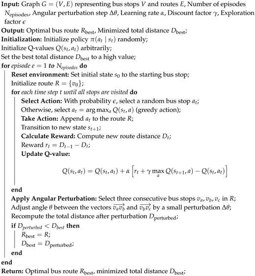
Reinforcement Learning (RL) combined with Angular Perturbation (AP) is a method used to minimize the total distance traveled while ensuring that all bus stops are visited exactly once. The environment is modeled as a graph G = ( V , E ) , where V represents the bus stops and E represents the routes between these stops. The goal of the RL agent is to learn an optimal route R that minimizes the total distance traveled.
The RL agent interacts with the environment by transitioning between states s t , where each state represents the sequence of bus stops visited at time step t. The agent selects actions a t , which involve choosing the next bus stop to visit. After each action, the agent receives a reward r t based on the change in the total distance of the route. The reward is defined as:
r t = D t 1 D t ,
where D t is the total distance after visiting the next bus stop, and D t 1 is the total distance before visiting the next stop. A positive reward is provided when the total distance decreases, thus encouraging the agent to find more efficient routes.
At each time step, the agent selects an action a t according to a policy π ( a t s t ) , which defines the strategy to select the next bus stop. Initially, the policy is random, but it is gradually refined over time through exploration and learning. The agent updates its knowledge using the Q-learning algorithm, where the Q-value Q ( s t , a t ) is updated according to the following equation:
Q ( s t , a t ) = Q ( s t , a t ) + α r t + γ max a Q ( s t + 1 , a ) Q ( s t , a t ) ,
where α is the learning rate, γ is the discount factor, and max a Q ( s t + 1 , a ) represents the expected future maximum reward for the next state s t + 1 .
After the RL agent learns a near-optimal route, Angular Perturbation (AP) is applied to further refine the solution. This involves selecting three consecutive bus stops v a , v b , and v c along the route, and adjusting the angle θ between the vectors v a v b and v b v c . The angle is perturbed by a small amount Δ θ to explore alternative configurations that may reduce the total distance. The perturbed route R is then evaluated, and if it results in a shorter total distance, the agent updates the current best route R best .
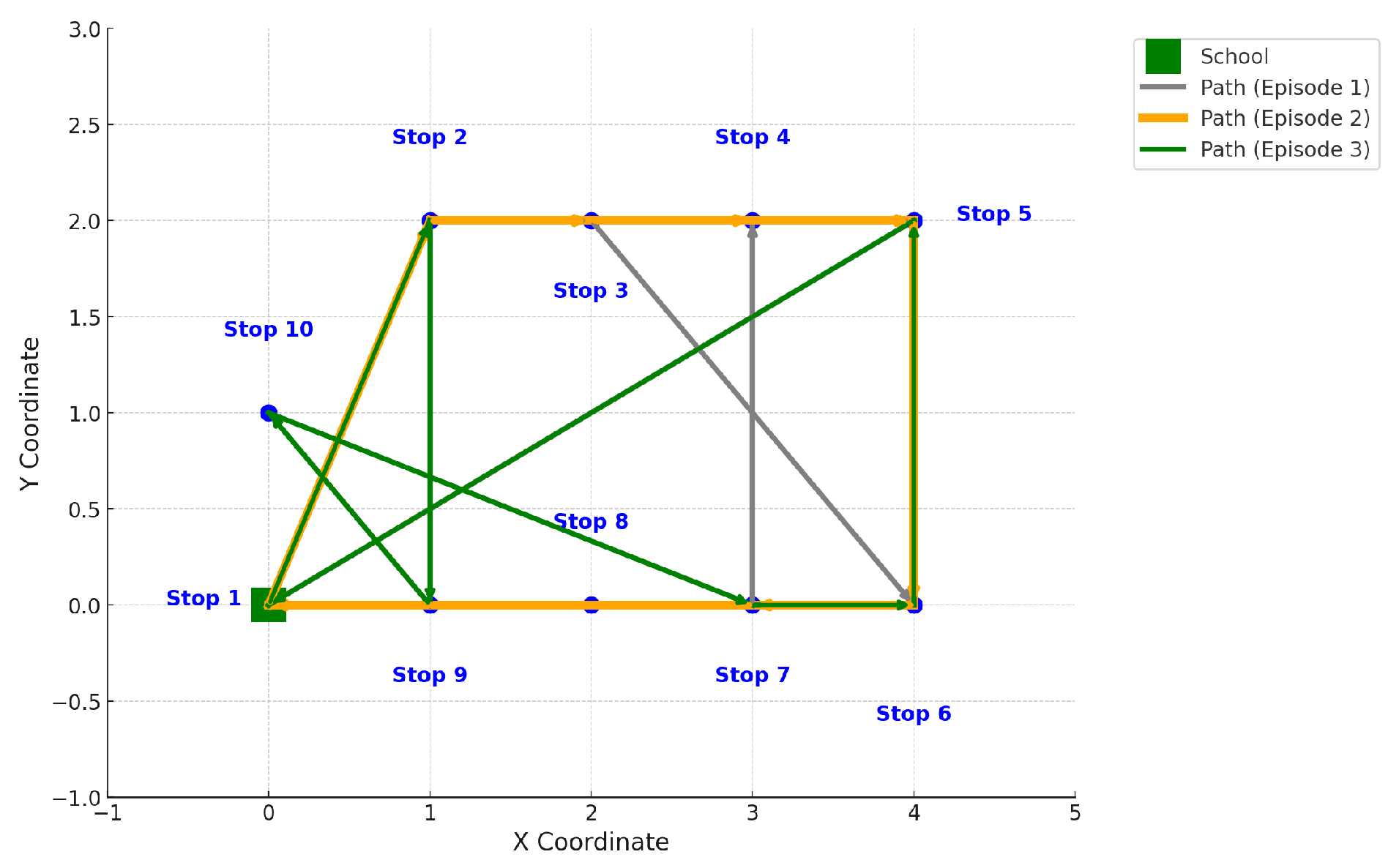
As shown in Figure 6, the diagram illustrates how Reinforcement Learning (RL) is applied to find an optimal route for a school bus visiting 10 stops. The different colored paths represent various episodes in the learning process, where the RL agent explores potential routes and gradually improves its actions based on the feedback it receives. The gray path (Episode 1) shows the agent’s initial exploration of the environment, where the bus follows a suboptimal and inefficient route, connecting the stops in a random or exploratory manner as the agent is still learning the structure of the environment and the rewards. In the orange path (Episode 2), there is noticeable improvement as the bus starts to follow a more structured route, reducing unnecessary detours. This indicates that the agent has learned from its earlier experiences and is adjusting its actions to improve efficiency. By the time it reaches the green path (Episode 3), the agent has further refined its strategy, and the bus follows a much more efficient and direct route between stops, suggesting that the RL agent is nearing an optimal solution.
This overall process, combining the learning capabilities of RL with the geometric refinement introduced by Angular Perturbation, allows the agent to continuously improve the bus route and minimize the total distance. The RL agent iteratively refines its policy and route through exploration and perturbation, ensuring an efficient solution.
Algorithm 3: RL-AP for SBR
Preprints 118492 i003

4. Computational Experiment

The anonymized dataset, obtained with the necessary permissions, was sourced from the databases of 10 schools in Kilifi County, Mombasa, Kenya. This section is divided into two parts: Section 4.1 presents the experiment that compares our proposed algorithm with the IBM CPLEX Optimizer, a robust tool for solving complex optimization problems such as the minimization of route distance in transportation, followed by an in-depth analysis of the results. Section 4.2 details an ablation study that evaluates the contribution of each component of the proposed algorithm to its overall performance. The experiments were carried out on a system equipped with an Intel Core i7 processor, 16GB of RAM, and a 500GB hard drive, ensuring computational efficiency and accuracy.

4.1. Computation Experiment With Angular Perturbation

In this section, we present the results of the computational experiment conducted with the inclusion of Angular Perturbation (AP) in all of our algorithms. Our objective is to evaluate the effectiveness of AP in optimizing school bus routes in 10 different cases. The performance of the algorithm was compared with and without AP to determine the impact of the perturbation technique on overall distance reduction.
Table 2 compares the performance of three different algorithms—GAACOSA-AP, BFSPSO-AP, RL-AP, and CPLEX—in optimizing school bus routes for 10 different schools in form of instances. The columns represent several key values for each school: the Existing Distance (ED) in kilometers (km), the Optimized Distance (OD) achieved by each algorithm, and the Objective Function (F = ED - OD), indicating how much each algorithm was able to reduce the original travel distance. The objective is to minimize the total travel distance, and the larger the objective function F, the better the algorithm has performed.
Looking at the results, the GAACOSA-AP algorithm consistently delivers the best performance across all 10 schools. For example, for School 1, the existing travel distance is 47.22 km, and GAACOSA-AP reduces it to 38.90 km, giving an objective function value of 8.32 km, which is the highest reduction among all algorithms. In contrast, BFSPSO-AP and RL-AP achieve smaller reductions, bringing the distance down to 42.30 km and 43.10 km, respectively, while CPLEX reduces it to 39.95 km. Although all algorithms manage to reduce the travel distance, GAACOSA-AP outperforms the others by achieving the largest reduction.
A similar pattern can be seen for School 3, where GAACOSA-AP reduces the distance from 55.60 km to 35.50 km, a reduction of 20.10 km. This is the largest reduction for this school, while CPLEX comes in second with a reduction of 19.80 km, and the other two algorithms provide slightly smaller reductions. While BFSPSO-AP and RL-AP still manage to significantly reduce the travel distance (by 18.40 km and 19.10 km, respectively), they consistently fall short of the results achieved by GAACOSA-AP.
The consistency of GAACOSAAP is notable across all schools. For example, in School 8, where the existing distance is 72.60 km, GAACOSA-AP reduces the distance by 19.75 km, again outperforming the other methods. This trend is maintained in all 10 schools, with GAACOSA-AP delivering the highest reductions in each case, demonstrating the algorithm’s superiority in optimizing school bus routes.
Although other algorithms, including BFSPSO-AP, RL-AP, and CPLEX, also perform well, their results are consistently less optimal when compared to GAACOSA-AP. For instance, in School 5, the existing distance of 29.15 km is reduced to 20.85 km by GAACOSA-AP, while BFSPSO-AP and RL-AP only reduce it to 22.60 km and 23.10 km, respectively. This consistent pattern of higher objective function values for GAACOSA-AP makes it clear that this algorithm provides the best overall performance for minimizing distances.
In summary, As presented in Table 3 we select the best and the second best performing algorithm from Table 2. The results show that GAACOSA-AP is the most effective algorithm for reducing school bus travel distances. Its consistent superiority in achieving the largest reductions across all schools highlights its robustness and efficiency in solving the School Bus Routing Problem. This suggests that GAACOSA-AP is a particularly suitable choice for applications where minimizing travel distances is a priority, offering both greater cost efficiency and better route planning.
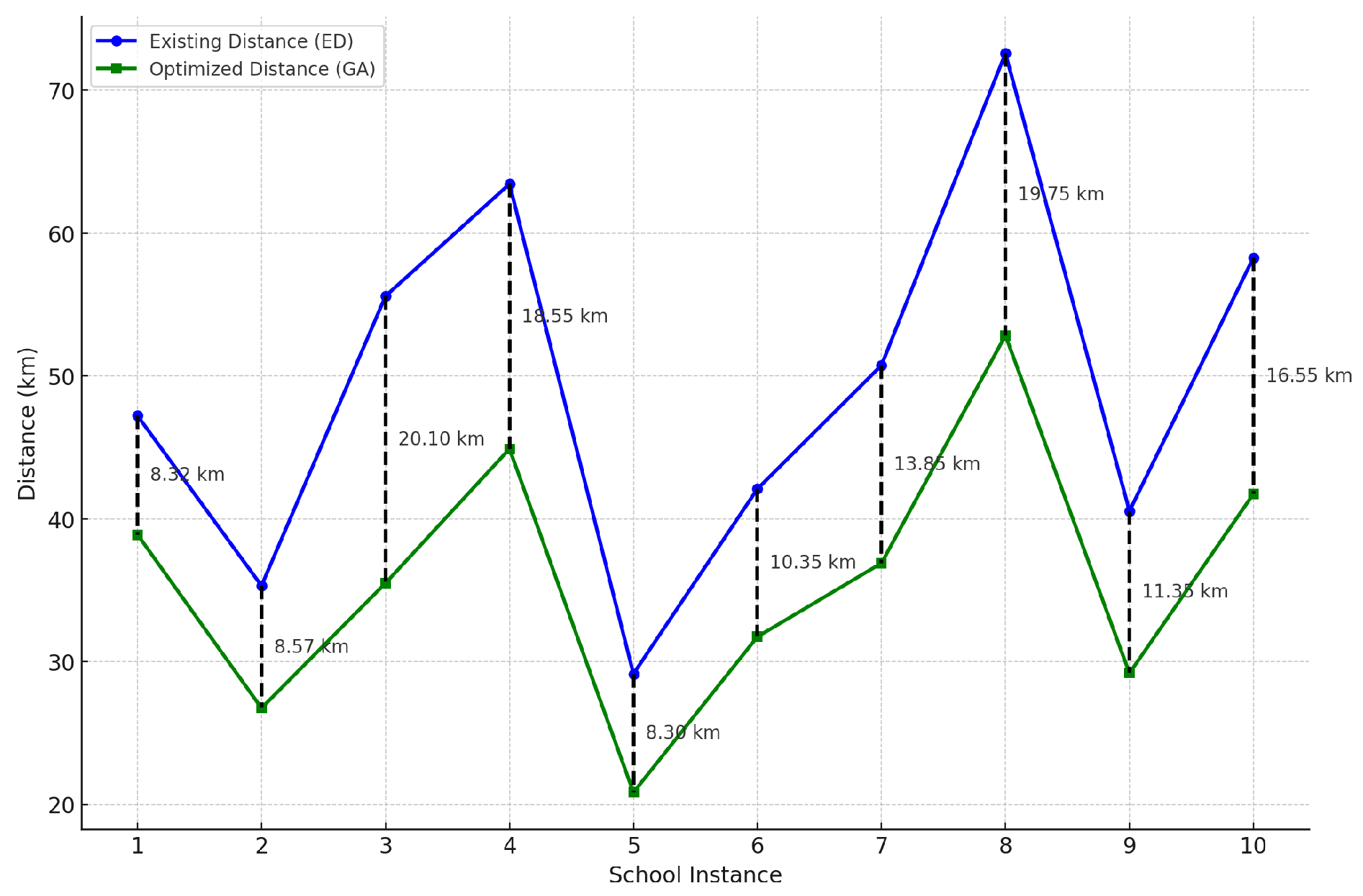
Figure 7 includes the difference values (in kilometers) between the Existing Distances (ED) and the Optimized Distances (GA). Each difference is displayed next to the vertical lines connecting the two curves, showing how much distance is reduced for each school instance.

4.2. Computation Experiment Without Angular Perturbation

To evaluate the effectiveness of Angular Perturbation (AP) in the GAACO-SA-AP algorithm, we conducted an ablation computational experiment. In this experiment, the Angular Perturbation (AP) strategy was removed from all proposed algorithms and a comprehensive computational analysis was performed. The experimental framework mirrors the structure outlined in Section 4.1, allowing for a direct comparison of results to assess the specific contribution of Angular Perturbation to the optimization performance.
As shown in Table 4, The results show that GAACOSA shortening it to GA consistently performs the best, achieving the lowest optimized distance in all 10 instances, which is highlighted in bold. For example, in School 1, the existing distance is 47.22 km, and GA reduces this to 40.50 km, resulting in a reduction of 6.72 km, outperforming both CPLEX (6.27 km) and the other algorithms (PSO: 4.12 km, RL: 3.42 km).
CPLEX follows closely behind, often providing the second-best results, with the difference between GA and CPLEX being relatively small in many cases. For example, in School 3, GA reduces the distance by 17.40 km, while CPLEX achieves a reduction of 18.50 km, slightly better in this instance. However, in the majority of cases, GA outperforms CPLEX by a narrow margin. In contrast, PSO and RL show consistently lower performance compared to GA and CPLEX. For example, in School 5, GA reduces the distance by 6.25 km, while PSO and RL only achieve reductions of 5.35 km and 4.95 km, respectively.
The performance of the algorithms varies between different schools. In some cases, the difference between GA and CPLEX is minimal, such as in School 9, where GA reduces the distance by 9.05 km and CPLEX by 8.45 km (a difference of 0.60 km). In other cases, such as School 7, the difference is more pronounced, with GA outperforming CPLEX by 1.60 km. The greatest reductions are observed in schools with higher distances, suggesting that more complex routes offer greater opportunities for optimization. For instance, in School 8, where the existing distance is 72.60 km, GA reduces the distance by 16.90 km, while CPLEX reduces it by 15.50 km.
In Figure 8, The algorithms compared are GA-AP (green), CPLEX (purple), and GA without AP (orange).
The X-axis represents the school instances, while the Y-axis corresponds to the vertical offsets for each algorithm (0 for GA-AP, 1 for CPLEX, and 2 for GA without AP). The Z-axis displays the difference in distance between the original and optimized routes (in kilometers).
From the plot, we can see that GA-AP consistently shows smaller differences in distances compared to GA without AP, indicating that the inclusion of Angular Perturbation improves route optimization. CPLEX performs similarly to GA-AP but generally falls between the two variants GA. This comparison highlights the advantages of using angular perturbation in reducing route distances more effectively.
For easy illustration, we select the first and second best perfroming algorthim from Table 4 and present their results highlighting the performance of the GA-ACO-SA algorithm versus CPLEX as show in Table 5. In all cases, the GA algorithm consistently outperforms CPLEX with smaller optimized distances, but the differences between the two algorithms are relatively small, ranging from 0.45 km to 1.40 km. The largest difference is seen in School 8, where GA achieves a distance of 55.70 km, compared to 57.10 km for CPLEX, a difference of 1.40 km. In most other schools, the differences are marginal, with the smallest difference of 0.45 km in School 1. These results suggest that while GA-ACO-SA performs slightly better in optimizing routes, CPLEX remains highly competitive in most cases, with only minimal performance gaps between the two algorithms.
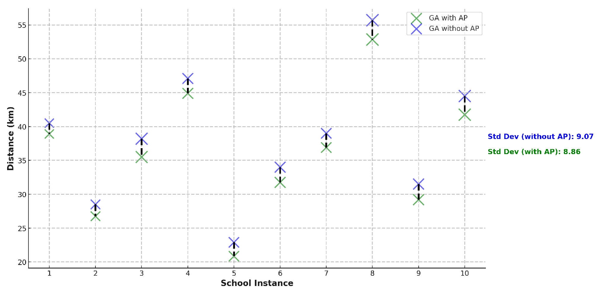
The markers in the graph Figure 8, illustrate the optimized distances for each school instance, with green markers representing the distances optimized using AP and blue markers representing the distances without AP. The size of the markers corresponds to the magnitude of the difference between the two approaches, with larger markers indicating a more significant disparity in performance. Additionally, dashed black lines connect the optimized distances for each school instance, visually depicting the difference between the two methods. Longer lines signify a greater benefit derived from using Angular Perturbation, as these instances show a more substantial reduction in travel distance.
The graph also includes standard deviation annotations, with the green text showing the standard deviation for the AP-optimized distances and the blue text for those without AP. The lower standard deviation in the AP approach (8.86) compared to the non-AP approach (9.07) highlights the more consistent and reliable outcomes produced by the use of Angular Perturbation. This reinforces the notion that AP not only results in shorter distances but also reduces variability across different school instances, ensuring a more stable and predictable optimization process. As illustrated in Table 5, we have selected the best and second-best results derived from the experimental findings presented in Table 4. This approach allows us to present the results in a more transparent and understandable manner for our readers.
In Table 6 ,this experimental results is derived from Table 2 and Table 4 and compares the results of the GAACOSA-AP algorithm with and without the AP component, highlighting the specific contribution that AP makes to the overall optimization process.
The ablation experiment revealed significant improvements in the optimized distances when Angular Perturbation (AP) was included in the algorithm. Across the 10 schools in the study, the version of the algorithm that incorporated AP consistently outperformed the version without AP. The differences between the two variants ranged from 1.60 km to 2.85 km, demonstrating that AP has a substantial impact on the ability of the algorithm to minimize travel distances.
For example, in School 3, the GAACOSA-AP algorithm with AP achieved an optimized distance of 35.50 km, while the version without AP resulted in a distance of 38.20 km. This difference of 2.70 km shows the clear benefit of including AP in the optimization process. Similarly, in School 8, the distance was reduced from 55.70 km without AP to 52.85 km with AP, a difference of 2.85 km.
Consistent improvements in all schools underscore the role that AP plays in the refinement of route geometry. Angular Perturbation adjusts the angles between consecutive bus stops, smoothing the route and reducing sharp turns that could increase the overall distance of travel. This enhancement is particularly important for complex routes with many stops or irregular layouts, where sub-optimal turns could lead to inefficiencies.
The greatest difference was observed in School 8, where AP reduced the distance by 2.85 km compared to the non-AP version. In this case, the complexity of the route probably contributed to the greater impact of AP, as the algorithm was able to significantly smooth the path and avoid inefficient detours. This suggests that AP is especially beneficial for routes with more intricate geometries.
Although AP generally provides significant improvements, the experiment also highlights cases where the gains are more marginal. In School 2, for example, the difference between the optimized distances with and without AP was only 1.75 km. Although still a significant improvement, it demonstrates that in simpler routing scenarios, the impact of AP may be less pronounced. In these cases, the base GA-ACO-SA algorithm without AP is already able to generate a near-optimal solution.
It is also important to consider the computational cost associated with angular perturbation. The addition of AP introduces a geometric component that requires additional computation time, particularly for larger instances with many bus stops. However, the improved optimized distances, as shown in the ablation study, suggest that the increased computational effort is justified by the reductions in travel distance. Although the results indicate that the performance gains provided by AP outweigh any additional time complexity, particularly in instances where distance reductions are substantial.
The average optimized distance reduction with angular perturbation is approximately 27. 12%, while the average optimized distance reduction without angular perturbation is approximately 22. 37%. This shows that the use of Angular Perturbation provides a significant improvement in the optimization process.
5. Comprehensive Analysis Using Clustering and K-Nearest Neighbor Evaluation

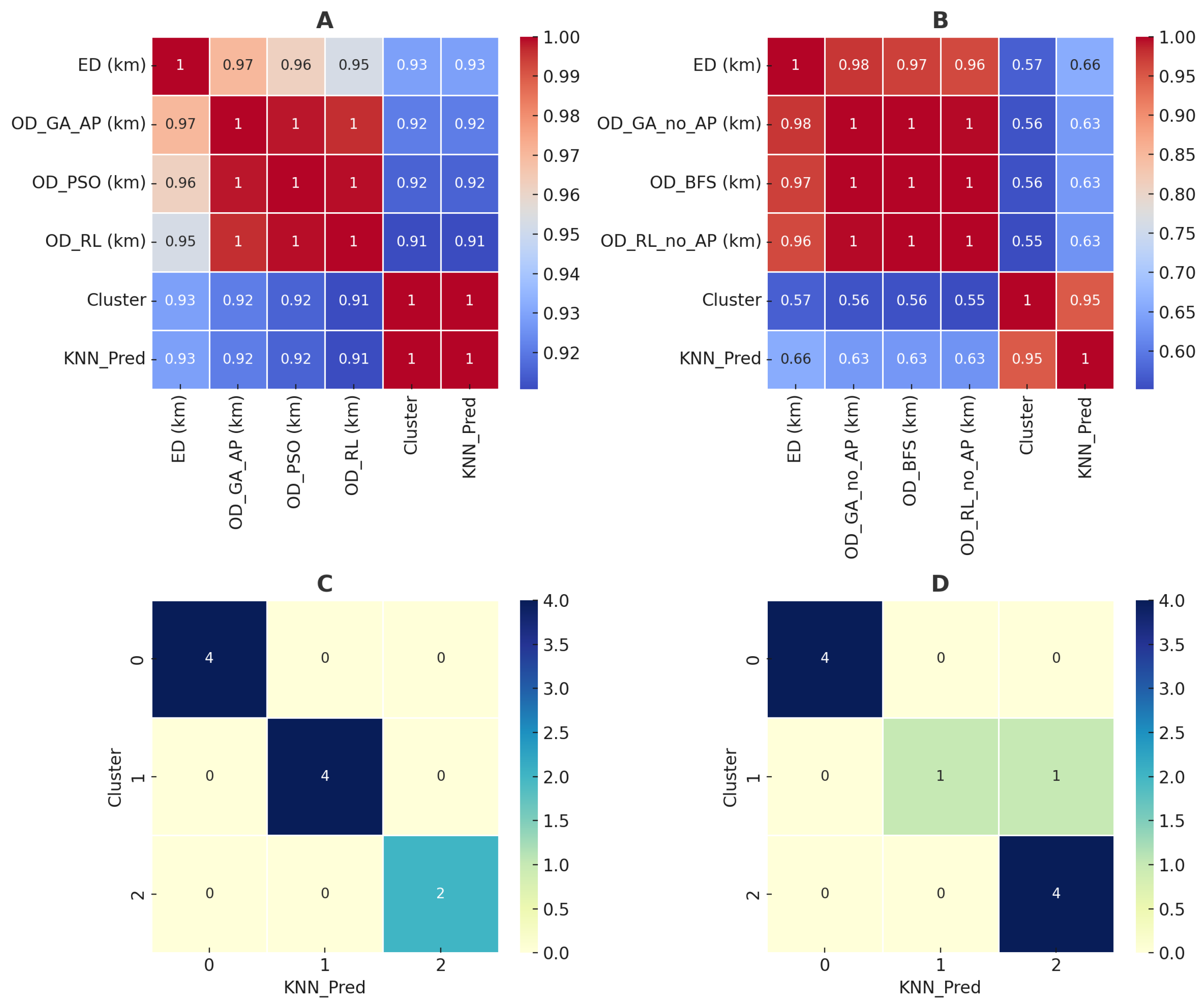
This section provides a comparative analysis : one that incorporates angular perturbation (AP) and the other without. The primary goal is to evaluate the impact of Angular Perturbation on enhancing the efficiency of various optimization techniques. The outcomes of these optimizations are analyzed through clustering techniques and validated using K-Nearest Neighbor (KNN) evaluation, visualized in four graphs labeled A, B, C, and D as illustrated in Figure 9.
Graph A and B depict correlation matrices showing how different optimization methods perform with and without Angular Perturbation. Graph A, representing optimization results with Angular Perturbation, demonstrates stronger correlations between methods like GAACOSA-AP and BFSPSO-AP, suggesting that AP increases consistency and reliability in optimization outcomes. The strong correlation between OD_GA_AP and OD_BFS/PSO indicates that these algorithms produce more aligned results when Angular Perturbation is applied. In contrast, graph B, showing results without AP, reveals weaker correlations, particularly between BFSPSO-AP and RL, indicating greater variability and inconsistency in the optimization results.
Graph C and D present the results of the K-Nearest Neighbor evaluation, assessing how well the clustering of optimized results is achieved. Graph C, which evaluates the clustering accuracy for data with Angular Perturbation, reveals distinct clusters with strong internal cohesion, indicating that the optimized routes form well-defined groups. In contrast, Graph D, representing clustering results without Angular Perturbation, shows some overlap between clusters, suggesting that the optimization results are less distinct and more difficult to separate. This confirms that Angular Perturbation not only enhances the optimization performance but also results in more structured and distinguishable clusters of optimized routes.
In conclusion, the analysis highlights that Angular Perturbation significantly improves the consistency and efficiency of school bus routing optimization. The clustering analysis underscores stronger correlations and more reliable optimization outcomes when AP is applied, while the KNN evaluation demonstrates clearer, more distinct clusters. These findings suggest that incorporating Angular Perturbation into metaheuristic optimization can lead to better-organized solutions, contributing to improved route efficiency and computational performance. Future work could explore larger datasets or expand the use of Angular Perturbation in other domains, such as logistics and transportation.

6. Conclusion and Future Work

In this study, we examined the effectiveness of the novel three-phase angular perturbation technique for metaheuristic-based school bus routing optimization, focusing on the influence of Angular Perturbation (AP) on route efficiency. Through a series of computational experiments, we evaluated the performance of our hybrid algorithm against the industry-leading optimization software, CPLEX, and other optimization techniques in multiple school scenarios. The results show that the GAACOSA-AP algorithm consistently outperforms its counterparts, achieving substantial reductions in travel distances, particularly for complex routes with numerous stops. The integration of Angular Perturbation was key to improving route geometry, reducing sharp turns, and enhancing overall path optimization.
While our approach has proven effective, there is room for improvement and further exploration. One key area for future research is the integration of Generative AI models with traditional optimization techniques. By leveraging AI-driven learning models, it may be possible to improve the generation of initial solutions in genetic algorithms, allowing the model to learn from historical data and generate more efficient initial populations. Furthermore, AI could be used to predict traffic patterns or student distributions, providing real-time updates and adaptive optimization as conditions change. This would allow for more dynamic, flexible route planning that adjusts on the fly.
Another potential area of future work is the development of explanable AI (XAI) models that can provide deeper insight into the decision-making processes behind route optimizations. This could help stakeholders understand why certain routes were chosen and build trust in the algorithms used. Furthermore,combining deep learning with optimization algorithms like GA-ACO-SA could further refine the solution space, reducing computation times and improving accuracy.
In conclusion, while the current study has highlighted the value of hybrid optimization approaches, future research integrating Generative AI, predictive modeling, and dynamic data updates offers exciting potential to further enhance the field of route optimization, not only for school buses but also for broader applications in logistics and transportation.

Author Contributions

Conceptualization, K.M and K.T.; methodology, K.M., M.F. and K.T.; software, E.C.; validation, K.M.; investigation, K.M and K.T.; resources, M.F. and K.T.; data curation, K.M. and T.K.; writing—original draft preparation, K.M.; writing—review and editing, K.M., M.F. and T.K.; visualization, K.M. and T.K; supervision, M.F. and T.K. All authors have read and agreed to the published version of the manuscript.

Funding

This research received no external funding

Institutional Review Board Statement

The study was conducted in accordance approved by the Technical University of Mombasa, Ethical Review Board (Approval code: TUM SERC MSC/015/2024) on 1st July 2024. It was also granted by the National Commission for Science, Technology and Innovation (NACOSTI), Kenya with license number NACOSTI/P/24/493548 on 22th July 2024. The dataset used in this research was facilitated by several school before commencement of the study, St.Patrick Academy and Junior School Kilifi, approved on 7th July 2024. Mkoroshoni Grace Missionary School Approved on 7th August 2024, another schools were St.Beatrice Academy,ST.Patrick Academy Nursery School, Ocean of Wonders Academy, Preparatory Academy, Kilifi Junior Academy, Little Angles Academy,Little Mountain Academy and St.Jude Academy

Informed Consent Statement

Not applicable.

Data Availability Statement

Upon request the data set will be shared.

Acknowledgments

We express our sincere gratitude to all those who have contributed to the completion of this work. Our appreciation extends to colleagues at the Institute of Computing and Informatics, Technical University of Mombasa for their invaluable support, guidance, and insights throughout the research process.

Conflicts of Interest

The authors declare no conflicts of interest.

Abbreviations

The following abbreviations are used in this manuscript in the order in which they appear throughout the text:
SBRP School Bus Routing Problem
NP-Hard Non-Deterministic Polynomial -Time Hardness
TSP Travelling Salesman Problem
VRP Vehicle Routing Problem
AP Angular Perturbation
GAACOSA-AP Genetic algorithm,Ant Colony Optimisation ,Simulated annealing - AP
BFSPSO-AP Breadth-First Search and Particle Swarm Optimization - AP
RL-AP Reinforcement Learning - AP
CPLEX Constraint Programming Linear Programming with Extensions
ED Existing Distance
OD Optimized Distance
OF Objective Function
KNN K-Nearest Neighbor
AI Artificial Intelligence
GEN AI Generative AI
XAI Explainable AI

References

  1. Dündar, H.; Ömürgönülşen, M.; Soysal, M. A Review on Sustainable Urban Vehicle Routing. Journal of Cleaner Production 2021, 285, 125444. [Google Scholar] [CrossRef]
  2. Miranda, D.M.; de Camargo, R.S.; Conceição, S.V.; Porto, M.F.; Nunes, N.T.R. A Metaheuristic for the Rural School Bus Routing Problem with Bell Adjustment. Expert Syst. Appl. 2021, 180, 115086. [Google Scholar] [CrossRef]
  3. Delussu, F.; Imran, F.; Mattia, C.; Meo, R. Fuel Prediction and Reduction in Public Transportation by Sensor Monitoring and Bayesian Networks. Sensors 2021, 21, 4733. [Google Scholar] [CrossRef] [PubMed]
  4. Calvete, H.I.; Galé, C.; Iranzo, J.A.; Toth, P. A Partial Allocation Local Search Matheuristic for Solving the School Bus Routing Problem with Bus Stop Selection. Mathematics 2020, 8, 1214. [Google Scholar] [CrossRef]
  5. Wang, X.; Tian, J. Dynamic Programming for NP-Hard Problems. Procedia Engineering 2011, 15, 3396–3400. [Google Scholar] [CrossRef]
  6. Ellegood, W.A.; Solomon, S.; North, J.; Campbell, J.F. School Bus Routing Problem: Contemporary Trends and Research Directions. Omega 2020, 95, 102056. [Google Scholar] [CrossRef]
  7. Plaisted, D.A. New NP-Hard and NP-Complete Polynomial and Integer Divisibility Problems. Theoretical Computer Science 1984, 31, 125–138. [Google Scholar] [CrossRef]
  8. Utama, D.M.; Dewi, S.K.; Wahid, A.; Santoso, I.; Pham, D. The Vehicle Routing Problem for Perishable Goods: A Systematic Review. Cogent Eng. 2020, 7, 1816148. [Google Scholar] [CrossRef]
  9. Sun, C. A Study of Solving Traveling Salesman Problem with Genetic Algorithm. In Proceedings of the 2020 9th International Conference on Industrial Technology and Management (ICITM), Oxford, UK, 11–13 February 2020; pp. 307–311. [Google Scholar] [CrossRef]
  10. Laporte, G. The Traveling Salesman Problem, the Vehicle Routing Problem, and Their Impact on Combinatorial Optimization. International Journal of Strategic Decision Sciences (IJSDS) 2010, 1, 82–92. [Google Scholar] [CrossRef]
  11. Ngoo, C.M.; Goh, S.L.; Sze, S.N.; Sabar, N.R.; Ahmad Hijazi, M.H.; Kendall, G. A Survey of Mat-Heuristics for Combinatorial Optimisation Problems: Variants, Trends and Opportunities. Applied Soft Computing 2024, 164, 111947. [Google Scholar] [CrossRef]
  12. Shang, P.; Yang, L.; Zeng, Z.; Tong, L. (Carol). Solving School Bus Routing Problem with Mixed-Load Allowance for Multiple Schools. Computers I& Industrial Engineering 2021, 151, 106916. [Google Scholar] [CrossRef]
  13. Tole, K.; Milani, M.; Mwakondo, F. Particle Swarm Algorithm for Improved Handling of the Mirrored Traveling Tournament Problem. Tehnički vjesnik 2021, 28, 1647–1653. [Google Scholar] [CrossRef]
  14. Bouzid, M.; Masmoudi, O.; Yalaoui, A. Exact Methods and Heuristics for Order Acceptance Scheduling Problem under Time-of-Use Costs and Carbon Emissions. Appl. Sci. 2021, 11, 8919. [Google Scholar] [CrossRef]
  15. Vieira, B.S.; Ribeiro, G.M.; Bahiense, L.; Cruz, R.; Mendes, A.B.; Laporte, G. Exact and Heuristic Algorithms for the Fleet Composition and Periodic Routing Problem of Offshore Supply Vessels with Berth Allocation Decisions. European Journal of Operational Research 2021, 295(3), 908–923. [Google Scholar] [CrossRef]
  16. Valle, C.A.; Martinez, L.C.; da Cunha, A.S.; Mateus, G.R. Heuristic and Exact Algorithms for a Min–Max Selective Vehicle Routing Problem. Computers I& Operations Research 2011, 38, 1054–1065. [Google Scholar] [CrossRef]
  17. Doerner, K.F.; Gronalt, M.; Hartl, R.F.; Kiechle, G.; Reimann, M. Exact and Heuristic Algorithms for the Vehicle Routing Problem with Multiple Interdependent Time Windows. Computers and Operations Research 2008, 35(9), 3034–3048. [Google Scholar] [CrossRef]
  18. Dordevic, M.; Tešić, R.; Todorović, S.; Jokić, M.; Das, D.K.; Stević, Ž.; Vrtagic, S. Development of Integrated Linear Programming Fuzzy-Rough MCDM Model for Production Optimization. Axioms 2022, 11, 510. [Google Scholar] [CrossRef]
  19. Gilpin, S.; Davidson, I. A Flexible ILP Formulation for Hierarchical Clustering. Artificial Intelligence 2017, 244, 95–109. [Google Scholar] [CrossRef]
  20. Podgorelec, D.; Žalik, B.; Mongus, D.; Vlahek, D. A New Alternating Suboptimal Dynamic Programming Algorithm with Applications for Feature Selection. Mathematics 2024, 12, 1987. [Google Scholar] [CrossRef]
  21. Gharbi, A. Exploring Heuristic and Optimization Approaches for Elevator Group Control Systems. Appl. Sci. 2024, 14, 995. [Google Scholar] [CrossRef]
  22. Irizar, I. A Mathematical Framework for Optimum Design and Operation of SBR Processes. Journal of Water Process Engineering 2021, 39, 101703. [Google Scholar] [CrossRef]
  23. Thinakaran, N.; Jayaprakash, J.; Elanchezhian, C. Greedy Algorithm for Inventory Routing Problem in a Supply Chain—A Review. Materials Today: Proceedings 2019, 16, 1055–1060. [Google Scholar] [CrossRef]
  24. Jin, T.; Huang, K.; Tang, J.; Xiao, X. Optimal Streaming Algorithms for Multi-Armed Bandits. In Proceedings of the 38th International Conference on Machine Learning; Meila, M., Zhang, T., Eds.; PMLR, 2021; Volume 139, pp. 5045–5054. Available online: https://proceedings.mlr.press/v139/jin21a.html (accessed on 13 September 2024).
  25. Holland, J.H. Adaptation in Natural and Artificial Systems; University of Michigan Press: Ann Arbor, MI, USA, 1975. [Google Scholar]
  26. Kirkpatrick, S.; Gelatt, C.D.; Vecchi, M.P. Optimization by Simulated Annealing. Science 1983, 220, 671–680. [Google Scholar] [CrossRef] [PubMed]
  27. Glover, F. Tabu Search—Part I. ORSA Journal on Computing 1989, 1, 190–206. [Google Scholar] [CrossRef]
  28. Zhai, J.; Song, D. Optimal Instance Subset Selection from Big Data Using Genetic Algorithm and Open Source Framework. J. Big Data 2022, 9, 87. [Google Scholar] [CrossRef]
  29. Rashidi, T.H.; Zokaei-Aashtiani, H.; Mohammadian, A.K. School Bus Routing Problem in Large-Scale Networks: New Approach Utilizing Tabu Search on a Case Study in Developing Countries. Transportation Research Record 2009, 2137(1), 140–147. [Google Scholar] [CrossRef]
  30. Thakkar, H.K.; Shukla, H.; Sahoo, P.K. Chapter 2 - Metaheuristics in Classification, Clustering, and Frequent Pattern Mining. In Cognitive Big Data Intelligence with a Metaheuristic Approach; Mishra, S., Tripathy, H.K., Mallick, P.K., Sangaiah, A.K., Chae, G.S., Eds.; Academic Press: 2022; Series Cognitive Data Science in Sustainable Computing, pp. 21–70. [CrossRef]
  31. Yin, R.; Lu, P. A Cluster-First Route-Second Constructive Heuristic Method for Emergency Logistics Scheduling in Urban Transport Networks. Sustainability 2022, 14, 2301. [Google Scholar] [CrossRef]
  32. Niculescu, V. On Generalizing Divide and Conquer Parallel Programming Pattern. Mathematics 2022, 10, 3925. [Google Scholar] [CrossRef]
  33. Lopes, C.; Rodrigues, A.M.; Romanciuc, V.; Ferreira, J.S.; Öztürk, E.G.; Oliveira, C. Divide and Conquer: A Location-Allocation Approach to Sectorization. Mathematics 2023, 11, 2553. [Google Scholar] [CrossRef]
  34. Li, Y.; Wang, J.; Liang, M.; Song, H.; Liao, J.; Lan, Y. A Novel Two-Stage Approach for Automatic Extraction and Multi-View Generation of Litchis. Agriculture 2024, 14, 1046. [Google Scholar] [CrossRef]
  35. Feng, J.; Wang, L.; Yu, H.; Jiao, L.; Zhang, X. Divide-and-Conquer Dual-Architecture Convolutional Neural Network for Classification of Hyperspectral Images. Remote Sens. 2019, 11, 484. [Google Scholar] [CrossRef]
  36. Kang, X.; Lin, X. Graph-Based Divide and Conquer Method for Parallelizing Spatial Operations on Vector Data. Remote Sens. 2014, 6, 10107–10130. [Google Scholar] [CrossRef]
  37. Kumari, M.; De, P.K.; Chaudhuri, K.; Narang, P. Utilizing a Hybrid Metaheuristic Algorithm to Solve Capacitated Vehicle Routing Problem. Results in Control and Optimization 2023, 13, 100292. [Google Scholar] [CrossRef]
  38. He, K.; Tole, K.; Ni, F.; Yuan, Y.; Liao, L. Adaptive Large Neighborhood Search for Solving the Circle Bin Packing Problem. Comput. Oper. Res. 2021, 127, 105140. [Google Scholar] [CrossRef]
  39. Yuan, Y.; Tole, K.; Ni, F.; He, K.; Xiong, Z.; Liu, J. Adaptive Simulated Annealing with Greedy Search for the Circle Bin Packing Problem. Comput. Oper. Res. 2022, 144, 105826. [Google Scholar] [CrossRef]
  40. Tole, K.; Moqa, R.; Zheng, J.; He, K. A Simulated Annealing Approach for the Circle Bin Packing Problem with Rectangular Items. Comput. Ind. Eng. 2023, 176, 109004. [Google Scholar] [CrossRef]
  41. He, K.; Tole, K.; Ni, F.; Yuan, Y.; Liao, L. Adaptive Large Neighborhood Search for Circle Bin Packing Problem. CoRR 2020, abs/2001.07709. Available online: https://arxiv.org/abs/2001.07709 (accessed on 17 September 2024).
  42. Tole, K.; Moqa, R.; Zheng, J.; He, K. A simulated annealing approach for the circle bin packing problem with rectangular items. Comput. Ind. Eng. 2023, 176, 109004. [Google Scholar] [CrossRef]
  43. Parra Inza, E.; Vakhania, N.; Sigarreta Almira, J.M.; Hernández Mira, F.A. Exact and Heuristic Algorithms for the Domination Problem. European Journal of Operational Research 2024, 313, 926–936. [Google Scholar] [CrossRef]
Figure 2. Demonstrating Routing Trajectory with Angular Pertubation Technique
Preprints 118492 g002
Figure 3. Simulated Annealing: Local Vs Global Optima
Preprints 118492 g003
Figure 4. Bus Picking Children with BFS Traversal with Minimal Path Intersections
Preprints 118492 g004
Figure 5. Bus Picking Children with BFS Traversal Multiple Path Intersections
Preprints 118492 g005
Figure 6. Reinforcement Learning for Optimal School Bus Routing
Preprints 118492 g006
Figure 7. Comparison of the Existing Distances (ED) and the Best Optimized Distances (GA) f
Preprints 118492 g007
Figure 8. Optimized Distances and Differences (With vs Without AP)
Preprints 118492 g008
Figure 9. Effect of Angular Perturbation on Optimization and Clustering Accuracy
Preprints 118492 g009
Table 2. Optimized Distances and Objective Functions for School Bus Routing (10 Schools)
S E D (km) O D GA F GA O D BFS F BFS O D RL F RL O D CPLEX F CPLEX
1 47.22 38.90 8.32 42.30 4.92 43.10 4.12 39.95 7.27
2 35.32 26.75 8.57 27.50 7.82 28.00 7.32 27.10 8.22
3 55.60 35.50 20.10 37.20 18.40 36.50 19.10 35.80 19.80
4 63.45 44.90 18.55 48.20 15.25 49.10 14.35 45.50 17.95
5 29.15 20.85 8.30 22.60 6.55 23.10 6.05 21.80 7.35
6 42.10 31.75 10.35 34.50 7.60 35.00 7.10 32.80 9.30
7 50.75 36.90 13.85 39.50 11.25 40.00 10.75 38.50 12.25
8 72.60 52.85 19.75 56.30 16.30 57.20 15.40 54.10 18.50
9 40.55 29.20 11.35 31.50 9.05 32.00 8.55 30.60 9.95
10 58.30 41.75 16.55 45.00 13.30 45.80 12.50 43.25 15.05
Table 3. Best and Second-Best Optimized Distances for School Bus Routing
S E D (km) Best Algorithm Second Best Algorithm Difference (km)
1 47.22 38.90 (GA) 39.95 (CPLEX) 1.05
2 35.32 26.75 (GA) 27.10 (CPLEX) 0.35
3 55.60 35.50 (GA) 35.80 (CPLEX) 0.30
4 63.45 44.90 (GA) 45.50 (CPLEX) 0.60
5 29.15 20.85 (GA) 21.80 (CPLEX) 0.95
6 42.10 31.75 (GA) 32.80 (CPLEX) 1.05
7 50.75 36.90 (GA) 38.50 (CPLEX) 1.60
8 72.60 52.85 (GA) 54.10 (CPLEX) 1.25
9 40.55 29.20 (GA) 30.60 (CPLEX) 1.40
10 58.30 41.75 (GA) 43.25 (CPLEX) 1.50
Table 4. Ablation Study: Optimized Distances Without Angular Perturbation (AP)
S E D (km) O D GA F GA O D BFS F BFS O D RL F RL O D CPLEX F CPLEX
1 47.22 40.50 6.72 43.10 4.12 43.80 3.42 40.95 6.27
2 35.32 28.50 6.82 28.80 6.52 29.10 6.22 27.95 7.37
3 55.60 38.20 17.40 39.00 16.60 38.70 16.90 37.10 18.50
4 63.45 47.10 16.35 49.50 13.95 50.00 13.45 47.80 15.65
5 29.15 22.90 6.25 23.80 5.35 24.20 4.95 23.50 5.65
6 42.10 34.00 8.10 35.50 6.60 35.80 6.30 34.60 7.50
7 50.75 39.00 11.75 40.80 9.95 41.20 9.55 39.90 10.85
8 72.60 55.70 16.90 58.50 14.10 59.10 13.50 57.10 15.50
9 40.55 31.50 9.05 33.00 7.55 33.40 7.15 32.10 8.45
10 58.30 44.50 13.80 46.70 11.60 47.20 11.10 45.30 13.00
Table 5. Ablation Study: Best and Second-Best Optimized Distances Without Angular Perturbation (AP)
S E D (km) Best Algorithm Second Best Algorithm Difference (km)
1 47.22 40.50 (GA) 40.95 (CPLEX) 0.45
2 35.32 28.50 (GA) 27.95 (CPLEX) 0.55
3 55.60 38.20 (GA) 37.10 (CPLEX) 1.10
4 63.45 47.10 (GA) 47.80 (CPLEX) 0.70
5 29.15 22.90 (GA) 23.50 (CPLEX) 0.60
6 42.10 34.00 (GA) 34.60 (CPLEX) 0.60
7 50.75 39.00 (GA) 39.90 (CPLEX) 0.90
8 72.60 55.70 (GA) 57.10 (CPLEX) 1.40
9 40.55 31.50 (GA) 32.10 (CPLEX) 0.60
10 58.30 44.50 (GA) 45.30 (CPLEX) 0.80
Table 6. Comparison of Best Results with and without Angular Perturbation
S E D (km) Best with AP (km) Best without AP (km) Difference (km)
1 47.22 38.90 (GA with AP) 40.50 (GA without AP) 1.60
2 35.32 26.75 (GA with AP) 28.50 (GA without AP) 1.75
3 55.60 35.50 (GA with AP) 38.20 (GA without AP) 2.70
4 63.45 44.90 (GA with AP) 47.10 (GA without AP) 2.20
5 29.15 20.85 (GA with AP) 22.90 (GA without AP) 2.05
6 42.10 31.75 (GA with AP) 34.00 (GA without AP) 2.25
7 50.75 36.90 (GA with AP) 39.00 (GA without AP) 2.10
8 72.60 52.85 (GA with AP) 55.70 (GA without AP) 2.85
9 40.55 29.20 (GA with AP) 31.50 (GA without AP) 2.30
10 58.30 41.75 (GA with AP) 44.50 (GA without AP) 2.75
Disclaimer/Publisher’s Note: The statements, opinions and data contained in all publications are solely those of the individual author(s) and contributor(s) and not of MDPI and/or the editor(s). MDPI and/or the editor(s) disclaim responsibility for any injury to people or property resulting from any ideas, methods, instructions or products referred to in the content.
Copyright: This open access article is published under a Creative Commons CC BY 4.0 license, which permit the free download, distribution, and reuse, provided that the author and preprint are cited in any reuse.
Prerpints.org logo

Preprints.org is a free preprint server supported by MDPI in Basel, Switzerland.

Subscribe

© 2024 MDPI (Basel, Switzerland) unless otherwise stated