1. Introduction
Structural damage and material ageing in carbon fibre composites significantly reduce the durability, maintainability, and safety of engineering structures such as wind turbine blades, aircraft wings, and boat hydrofoils. Timely and accurate structural assessments can prevent catastrophic failures and economic losses. Moreover, early detection of deterioration can alleviate the financial burdens associated with maintenance. Traditional laboratory-based SHM methods have been developed to monitor damage-sensitive features such as stress and strain at critical points, alongside electromechanical impedance techniques and vibration analysis. SHM strategies typically focus on five key aspects: damage detection, localization, classification, evaluation, and prediction of remaining functional life [
1].
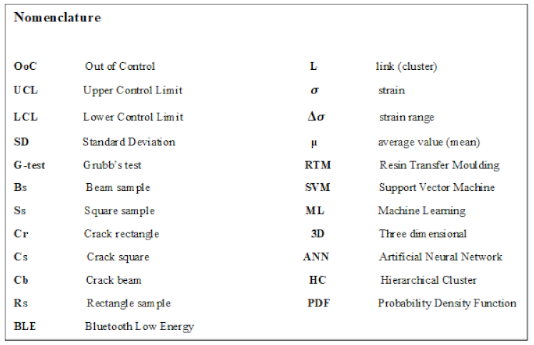
Monitoring composite materials via laboratory equipment, however, is both labour-intensive and environmentally taxing. Machine learning (ML) presents an appealing alternative, offering faster and more cost-effective predictions of material properties. ML enables robust statistical modelling and simulations, providing comprehensive insights into material performance under varying conditions, which would otherwise be challenging to capture through laboratory tests. Consequently, ML has garnered increasing attention in SHM applications, from fundamental property predictions [
2,
3] to experimental design [
4]. Through algorithmic approaches, ML facilitates high-throughput recognition and quantification of material damages.
Numerous studies demonstrate the success of ML in material science. For instance, Kabbani et al. [
5] achieved 90% accuracy in testing unidirectional fibreglass polypropylene using artificial neural networks (ANN), while Liu et al. [
6] optimised the algorithm for failure detection in woven composites. Other studies have applied support vector machines (SVM) [
8] and genetic algorithms [
7] to predict mechanical properties and material defects. Despite these advances, computational and statistical challenges persist, including scalability, data imbalance, small sample sizes, and high dimensionality.

2. Materials and Methods
The fabric structure evaluated in this study is layer-to-layer 3D woven [
17] that contains four wefts, six warp and six binders in the unit cell. To transform this fabric into a composite material, two resin systems (R1 and R2) are used within two different shapes of 3D preform (square & rectangle). R1 indicates the Prime 37 epoxy system, whereas R2 is a Pro-set epoxy system. Consolidation via resin transfer moulding (RTM) [
18] builds a solid carbon fibre-reinforced matrix. Carbon fibre-reinforced composite was used in the vessel’s interior. The material proved to have a better resistance in marine environments [
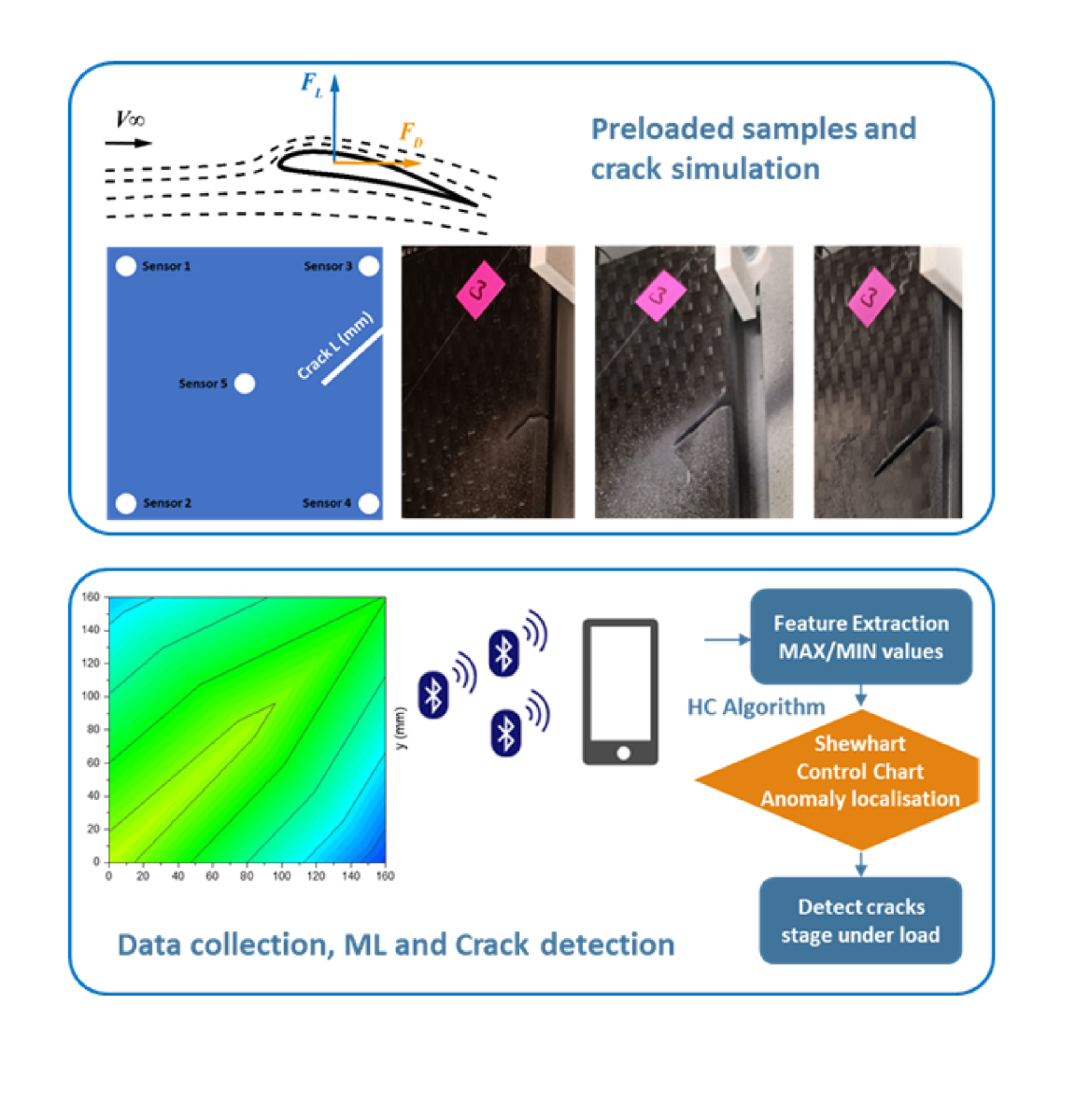
19]; the smooth external surface of the components is within the limit of dirt and subsequently, they are less susceptible. The material also expected to use as a composite boat hydrofoil that may experience different forces due to velocity changes, pressure and fluid’s viscosity. Generally, lift and drag forces could be exerted on the hydrofoil submerged in a stream flow. The hydrofoil surface is subjected to drag force by the fluid due to uneven pressures and viscous friction [
20]. Normally, fluid movement over the hydrofoil creates two different zone of fluid velocity due to the angle of attack and the camber. The differences between the velocity of the fluid particles at the higher and lower surface of the hydrofoil generate a low-pressure zone at the upper surface and a high-pressure zone at the lower surface. Uneven pressure distribution between the upper and lower surface of the hydrofoil generates the lift force [
21].
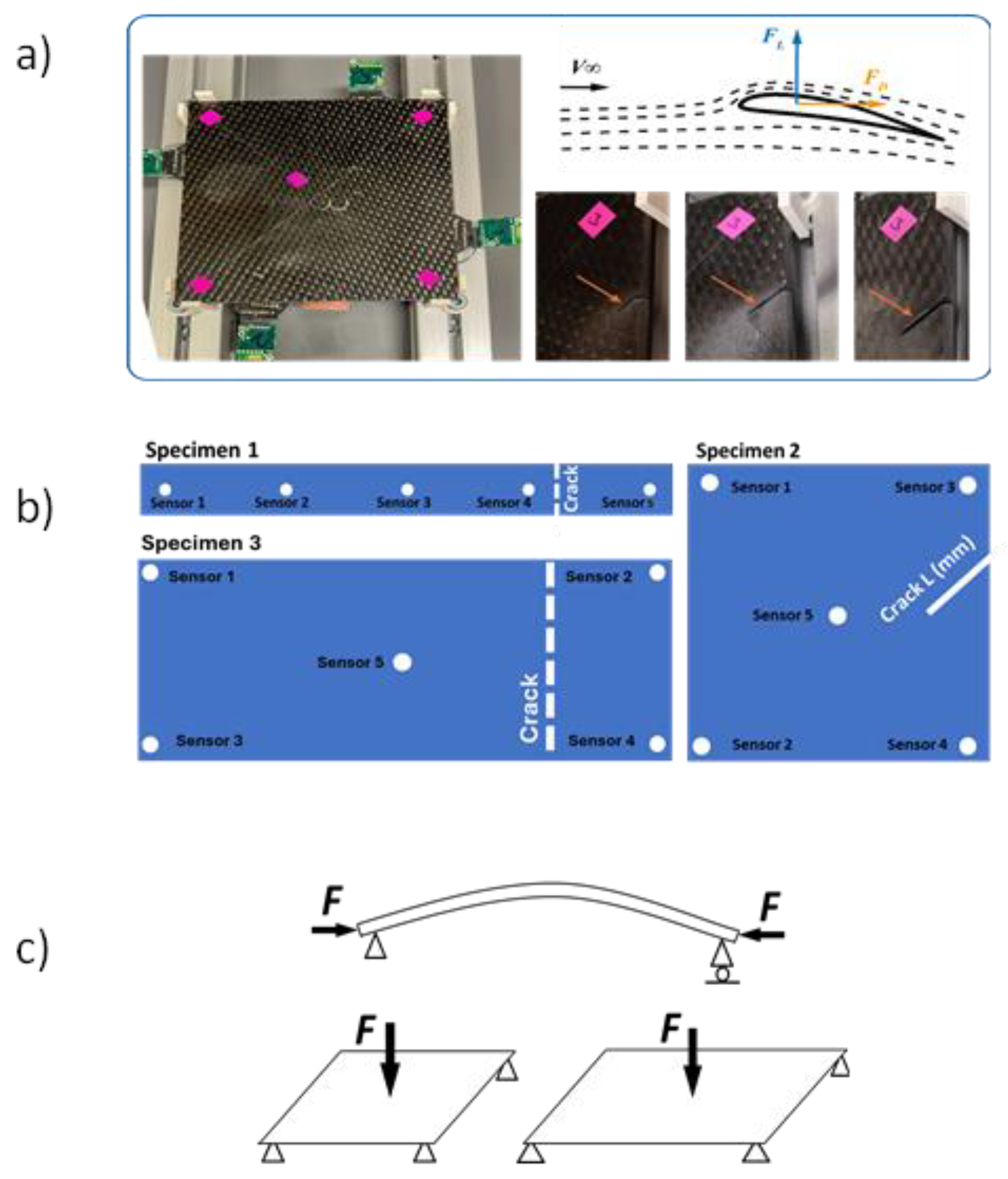
In this work, we use three samples cut from the 3D layer-to-layer composite material discussed above (
Figure 1a). Specimen one was a beam (Bs), two-point bending test was performed using a uniaxial experimental setting to determine the strain of the specimens (
Figure 1b). When a beam experiences a bending moment, it will change its shape and internal stresses will be developed (
Figure 1c). The second specimen was a rectangle sample (Rs) of 3D composite with a dimension of 160 x 340 mm that was instrumented with five strain gauge sensors and subjected to controlled loads. The strain samples were recorded as a function of fracture development when eleven cracks developed between 3,4 and 5. The third specimen was a square sample (Ss) with a dimension of 160 x160 mm that was equipped with another five strain gauges when ten surface cracks developed between sensors three and four.
In previous discussions, it was noted that various forces from water flow cause dynamic stress on hydrofoil structures. Bluetooth Low Energy (BLE) technology [
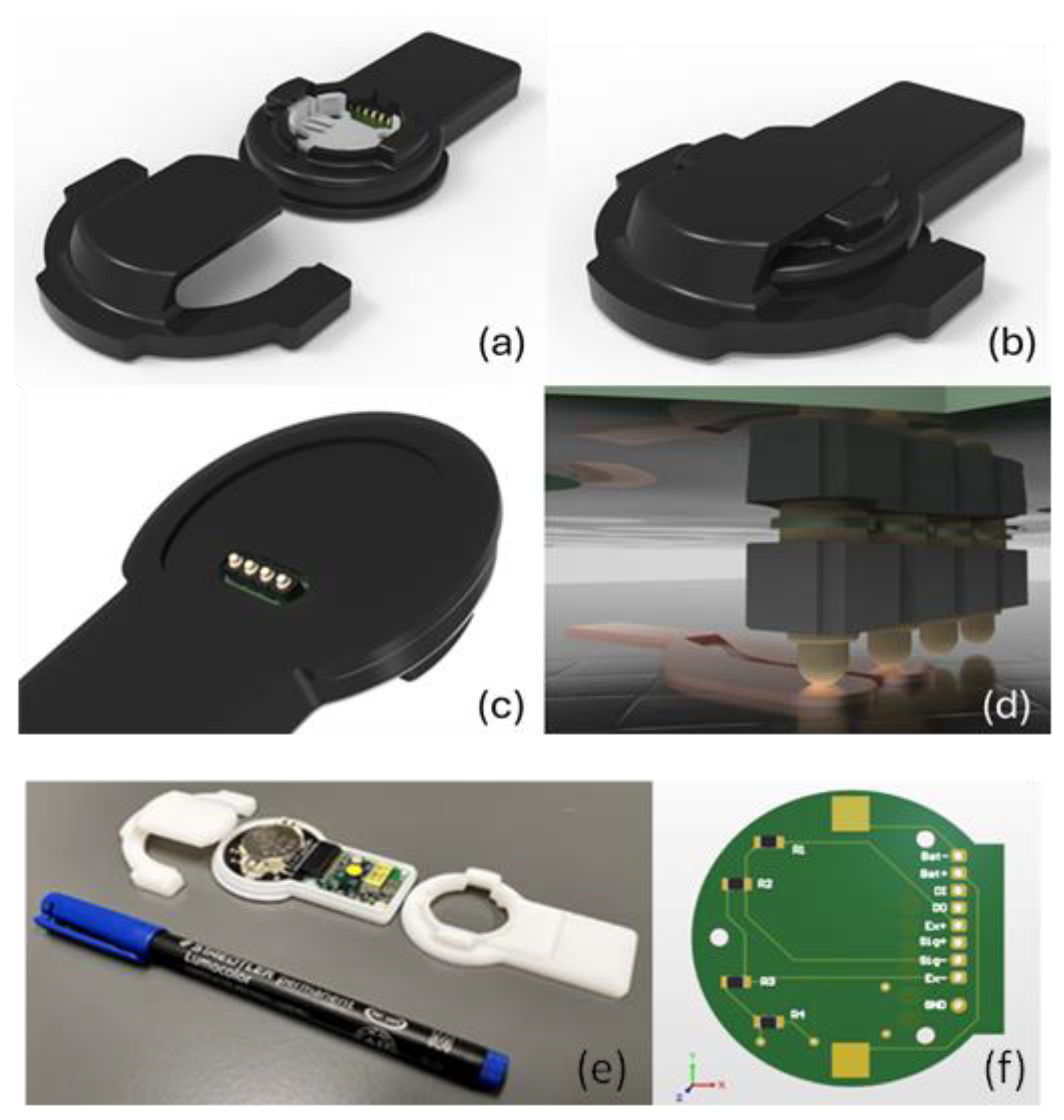
22] represents a new generation of Bluetooth-based strain gauge sensors that offer several advantages for monitoring hydrofoil structures. These sensors can be easily mounted on the inner surfaces of the hydrofoil without the need for complex wiring, making them suitable for underwater scenarios. In the current study, the sensor system is a compact module that houses the BLE (
Figure 2). The module includes a bridging board, a Bluetooth transmitter board B24-SSBX-A, and a strain gauge sensor. Importantly, it is designed that the coin-cell battery to be replaced without affecting the system’s functionality.
A compact and low-profile enclosure was designed to house the electronics module and a battery. The enclosure aligns and supports the spring-loaded connector, ensuring consistent contact with the strain gauge sensors during use. This modular configuration and its enclosure allow for easy disassembly and replacement of parts, maintenance, battery changes, and adaptation to various locations.
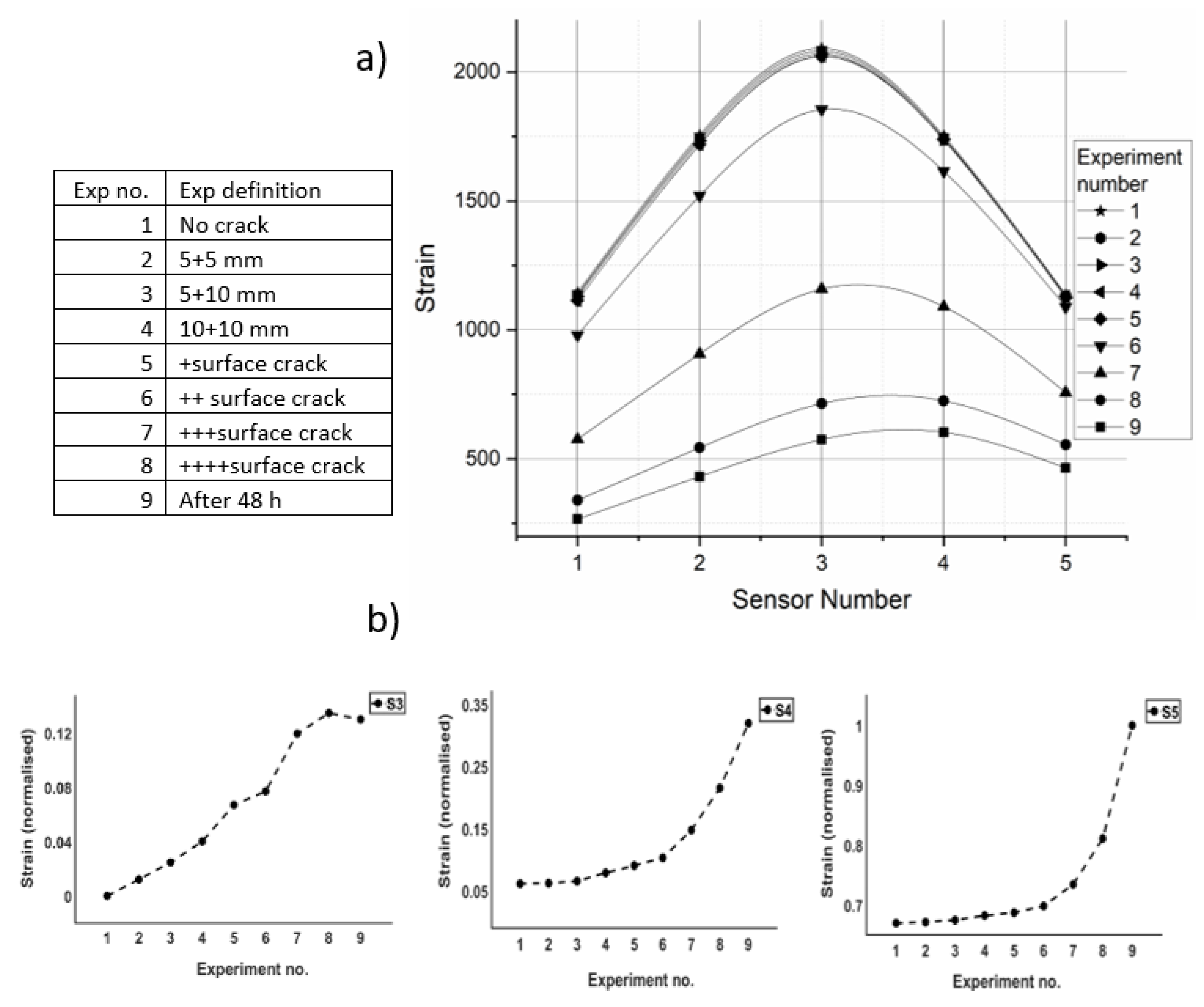
The transmitting board and the strain gauge sensor are connected via a bridging board. To provide the highest sensitivity to strain changes, strain gauges were integrated in a half-bridge Wheatstone configuration, where two active strain gauges are used in place of two of the bridge’s four resistors. This configuration can measure any variations in resistance, which can be caused by small strain changes or gauge deformation. The sensor outputs with various lengths and surface cracks developed are shown in
Figure 3, where the average strain value for each sensor was determined.
The BLE sensor value deviates from its mean around the crack zone when the fracture increments. The initial laboratory experimental results show that the sensors with a continuous increase in the strain indicate the presence of a crack. Those sensors with a greater distance may show a fluctuation in stain outputs (
Figure 3b). In this study, two above concepts are the basis for crack localisation which will be discussed in the next sections.
3. Computational Technique and Framework
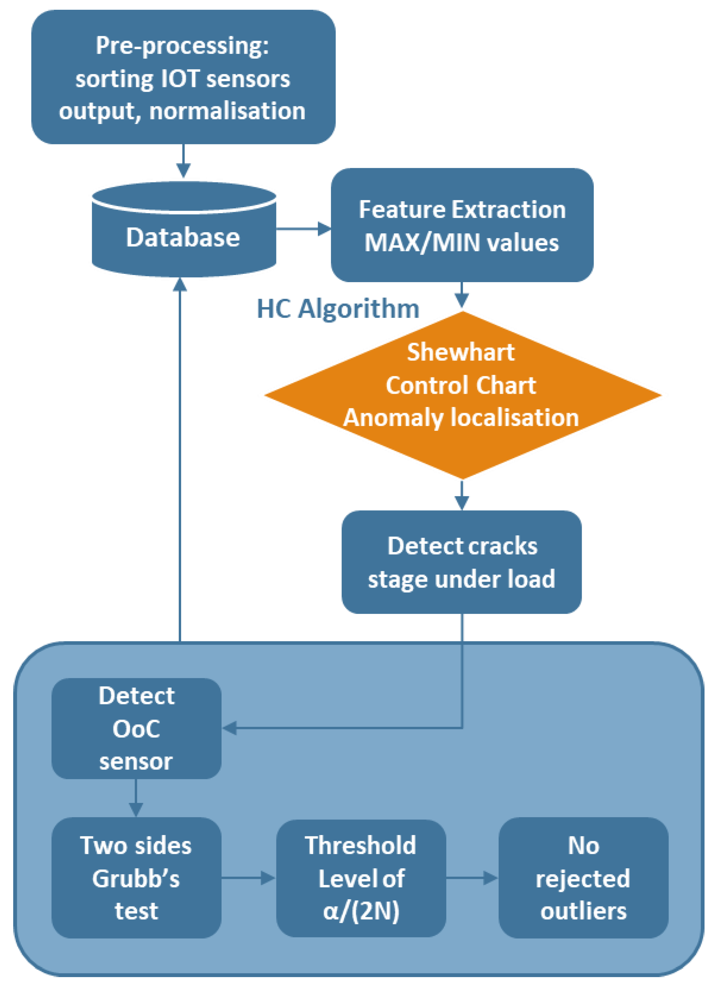
The study framework proposes three different algorithmic and statistical techniques to identify cracks and also classify them. All procedures are time-independent. Diagram one shows the fracture detection framework, which localises and predicts the fracture via machine learning algorithms.
This section is organised into three units. Initially, the Shewhart Control Chart [
23] was employed to detect anomalies in sensors with non-random conditions [
24], where healthy sample behaviour is also exhibited. Section two defines the Hierarchical Clustering algorithm to classify and train a model based on observations of incongruities in sensor output. Furthermore, Grubbs test [
25] with the corresponding threshold values receives the classified cracks at the next stage. The threshold values then define a boundary between the tolerance interval [
26] and the destructive fracture population.
Diagram 1.
Fracture detection framework: First, the data will be pre-processed, including splitting the output from BLE sensors and normalising it. The prominent features of the sensor output (such as max and mean) can then be extracted. Next, a control chart will be used to identify the location of fractures. At this stage, any incongruous sensor will have its output fed into the HC algorithm to identify the level of cracking. Subsequently, observations classified in the previous stage will be examined by GT for outlier rejection.
3.1. Sensor Control Limit
Shewhart control charts are well-known tools for identifying potential out-of-control (OoC) states [
27]. The basic principle of the chart is to detect instances where there is an unnatural deviation between parameters [
28]. In general, the chart maintains a centerline as the mean of the process, which can be controlled with an upper control limit (UCL) and a lower control limit (LCL) set at ±3σ, respectively [
29]. The conventional sigma value can be a moving average, range measurement, standard deviation (SD), or other attributes as required by the system to measure [
24,
30]. The process is considered in control or a stable phase if the measurement value fluctuates between the LCL and UCL, and out of control when a single observation is beyond the designated boundary [
31]. In the current study, the standard deviation has been used to determine how far each BLE sensor’s output has been located from its mean value when the cracks are developed [
32]. Based on our observation of multiple data sets, the sensor’s standard deviation closer to the crack exceeds the boundary of UCL/LCL. This feature helps to localise fractures.
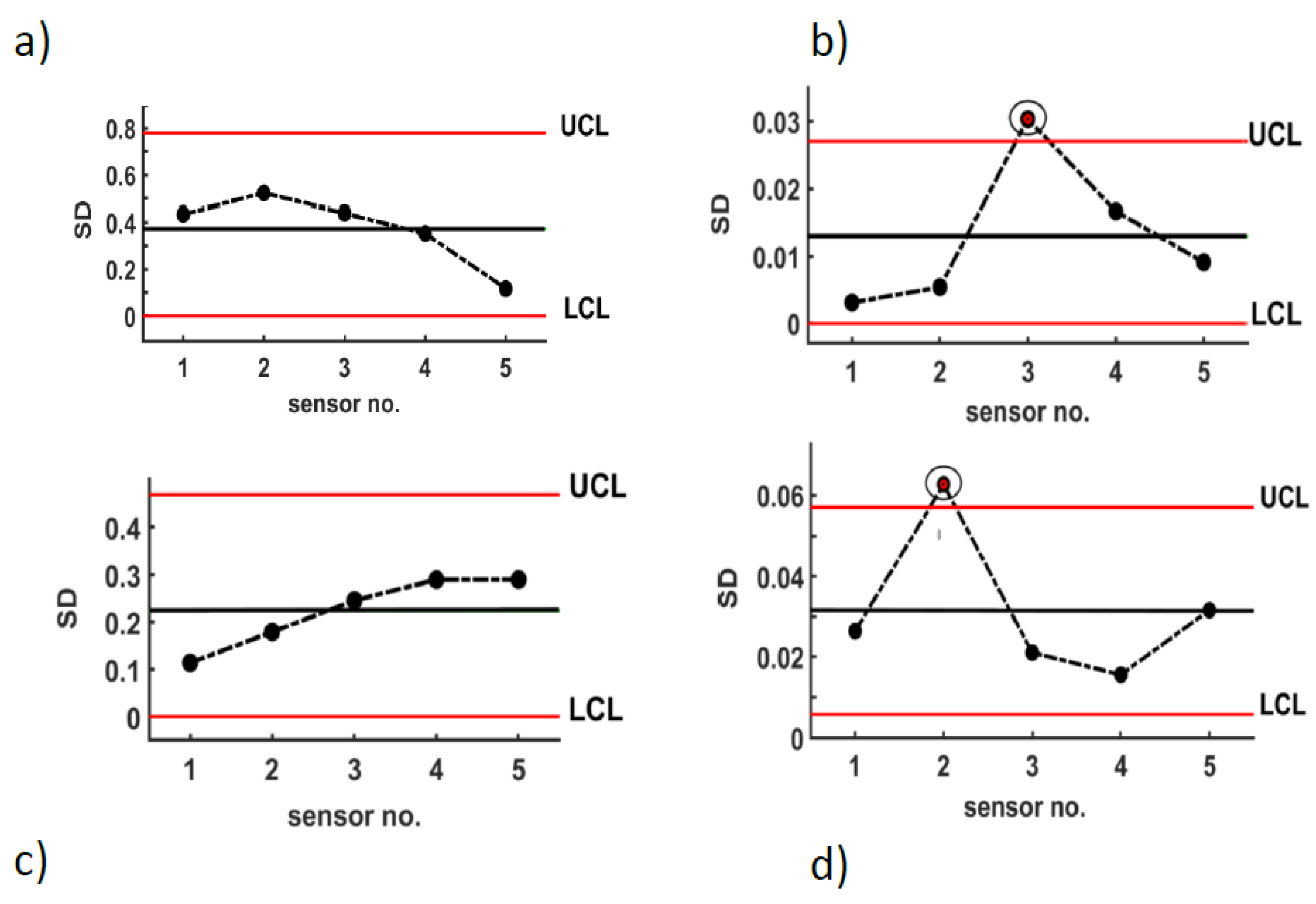
Figure 4 compares five sensors with loads (healthy sample) and the same sensors when cracks developed through the specimen (damaged sample).
Figure 4.
a) Comparing five sensors’ outputs for Rs before crack development (sensors under load but in normal phase). b) Anomalies sensors after crack development through Rs. c & d) comparing five sensor outputs for Ss before and after crack development respectively. As discussed above, a sensor close to cracks usually appears out of the UCL/LCL interval.
The Shewhart Charts can be implemented on all the sensor channels simultaneously. If the output of each sensor is x, and it normally distributed with mean of m and variance of SD, so the confidence interval will be:
where SD , n= number of fracturs and x̄ is average value of x.
3.2. Agglomerative Hierarchical Cluster Algorithm
The primary purpose of using unsupervised learning algorithms is to identify and categorise fractures to assess crack levels. This method generates significant clusters at different levels of a hierarchy. Data obtained from deviant BLE sensors will be fed into the HC algorithm for further classification. To group similar BLE outputs, a measurement is required. This measurement can be the distances relative to each other [
33,
34,
35,
36], meaning that pairs of sensor observations with closer distances could be grouped in similar clusters. In this study, the Chebyshev distance [
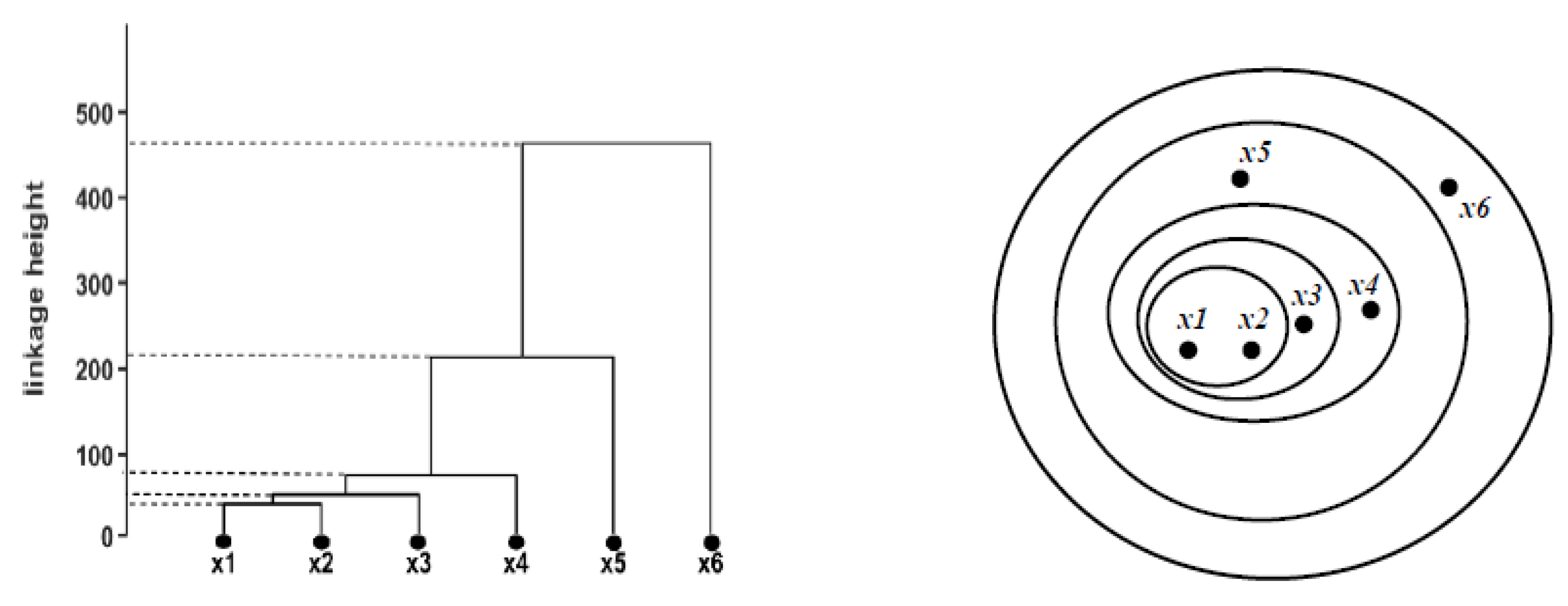
37] between data points is calculated. The measurement between points A and B is shown in the equation. This process continues until the intervals between all the observations are calculated and the entire BLE output is organised into various clusters. The visual representation of hierarchical clusters is commonly referred to as a dendrogram [
38], as shown in
Figure 5. The ultrametric topology illustrates how the fracture observations are developed. All clusters eventually link to each other to generate larger clusters until all observations in the original dataset are linked together [
34,
35]. The height of each link indicates the distance between the two points that are joined, where a shorter link between two objects represents a closer distance (and similarity), and a higher link shows dissimilarity between objects [
33].
Figure 5.
A dendrogram of six initial surface cracks (left), and equivalent Venn diagram (right). The dendrogram shows classificatory relationships between samples. This can be seen that the height of links increases when there is a progression in crack depth.
Figure 5.
A dendrogram of six initial surface cracks (left), and equivalent Venn diagram (right). The dendrogram shows classificatory relationships between samples. This can be seen that the height of links increases when there is a progression in crack depth.
3.2. Grubb’s Test
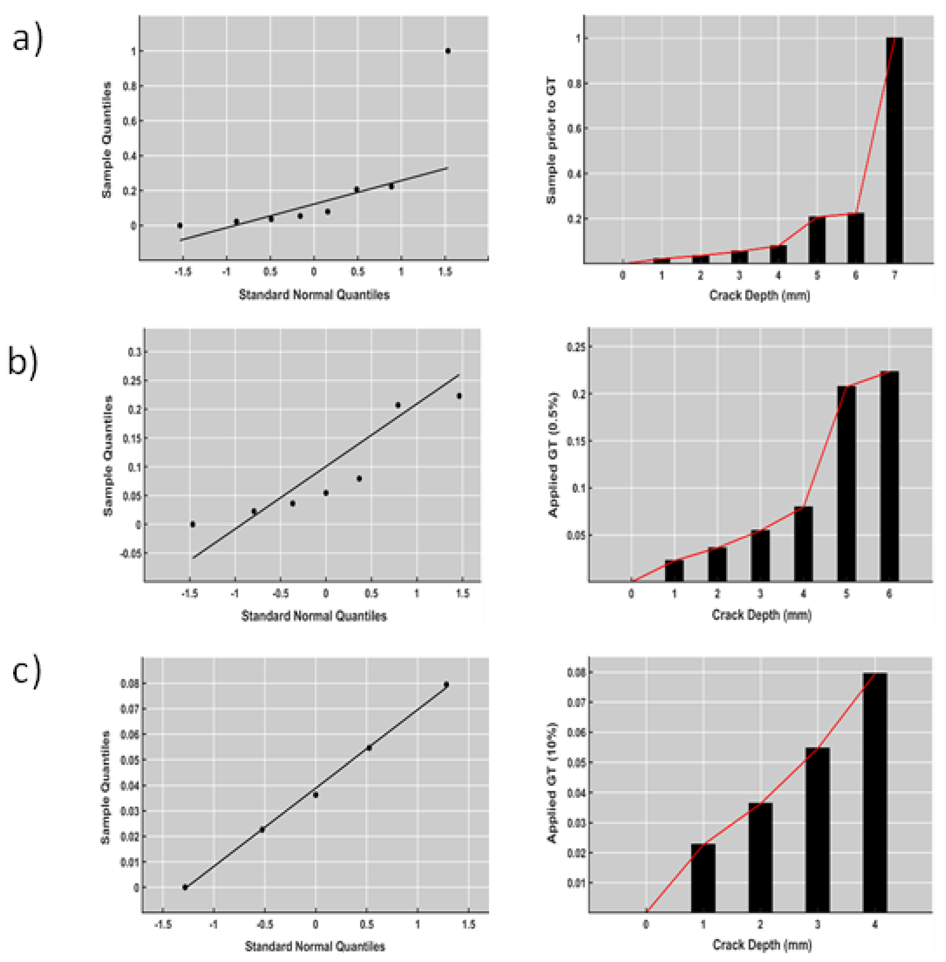
The sensor near the point of fracture shows an increase in strain measurements when cracks start to form. To prevent deeper cracks, a statistical test is used to identify outliers, such as crevasses, by setting a threshold condition. Grubb’s test (G-test) is employed to detect outliers from the previously categorized high-consequence observations by setting a threshold α. The test continues to reject outliers in each cycle until no exceptional data is found (refer to
Figure 6). The underlying theory of Grubbs’ test is that the observations are normally distributed. The G-statistic test is calculated for the out-of-control (OoC) BLE sensor output as follows:
Where
is the sensor outputs including healthy (without damage) observation and various depth crack’s sample,
is the mean value of the observation and
is standard deviation of data. Any result obtains from G-test and greater than
critical value will be eliminated in each cycle. The critical value can be determined as follow:
The
is a significant level that can be defined via
where
is condition threshold. The conventional value for
is 0.5, i.e., 95% of observations are in confident level and consider non-outlier [
42]. However, in current study, to avoid potential hazards at early stage, another threshold (10%) is evaluated. A reasonable concern is that a composite material test could contain more than one outlier that can call median hazard observation. GT threshold increments could assist in avoiding system failure in the recognition of unusual observations before main fractures.
Figure 6.
a) Normal probability plot of developed cracks prior to GT application. b) & c) The same samples after applying GT threshold (α)- (0.05 % and 10%) with 90% & 99.5 % confidence respectively.
Figure 6.
a) Normal probability plot of developed cracks prior to GT application. b) & c) The same samples after applying GT threshold (α)- (0.05 % and 10%) with 90% & 99.5 % confidence respectively.
4. Discussion and Results
In
Section 3.1, we discussed the use of the Shewhart control chart to pinpoint damage. This chart utilizes average values and standard deviation to detect deviations in sensor output from the mean or change point.
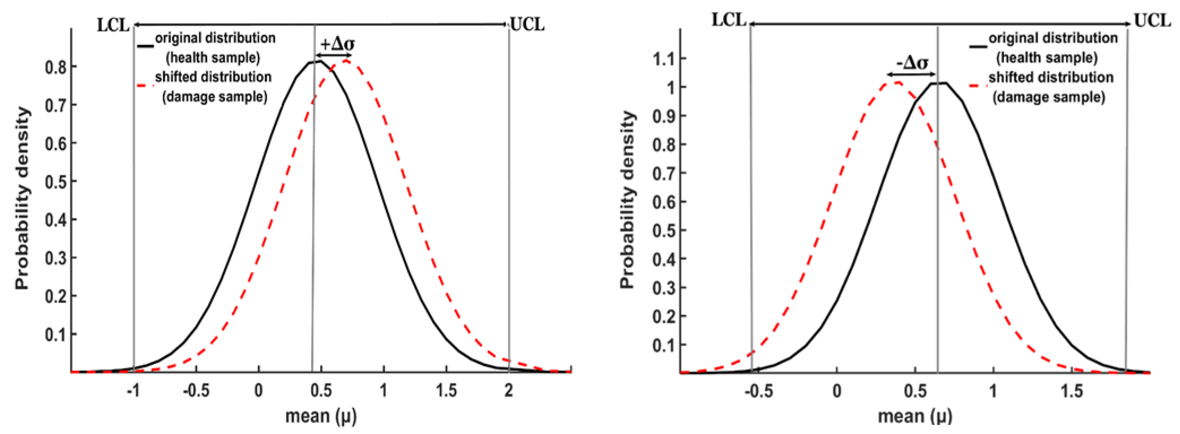
Figure 7 illustrates the comparison between the healthy and damaged sample mean intervals, which are determined by the lower and upper control limits (LCL and UCL). The Shewhart chart is used to monitor the sensor output within these boundaries, and any deviation beyond this interval could indicate an abnormal situation. Therefore, if a sensor’s distribution value shifts from m to m+Δσ, as shown in
Figure 7, it would be considered irregular.
LCL and UCL control limits are completely flexible and obey the sensor outputs. Each sensor provides various mean and SD values, that could result in non-identical Δσ and control limit assumptions. However, studies [
31,
43] proved that neither the number of observations nor stringent control limit is effective on OoC finding.
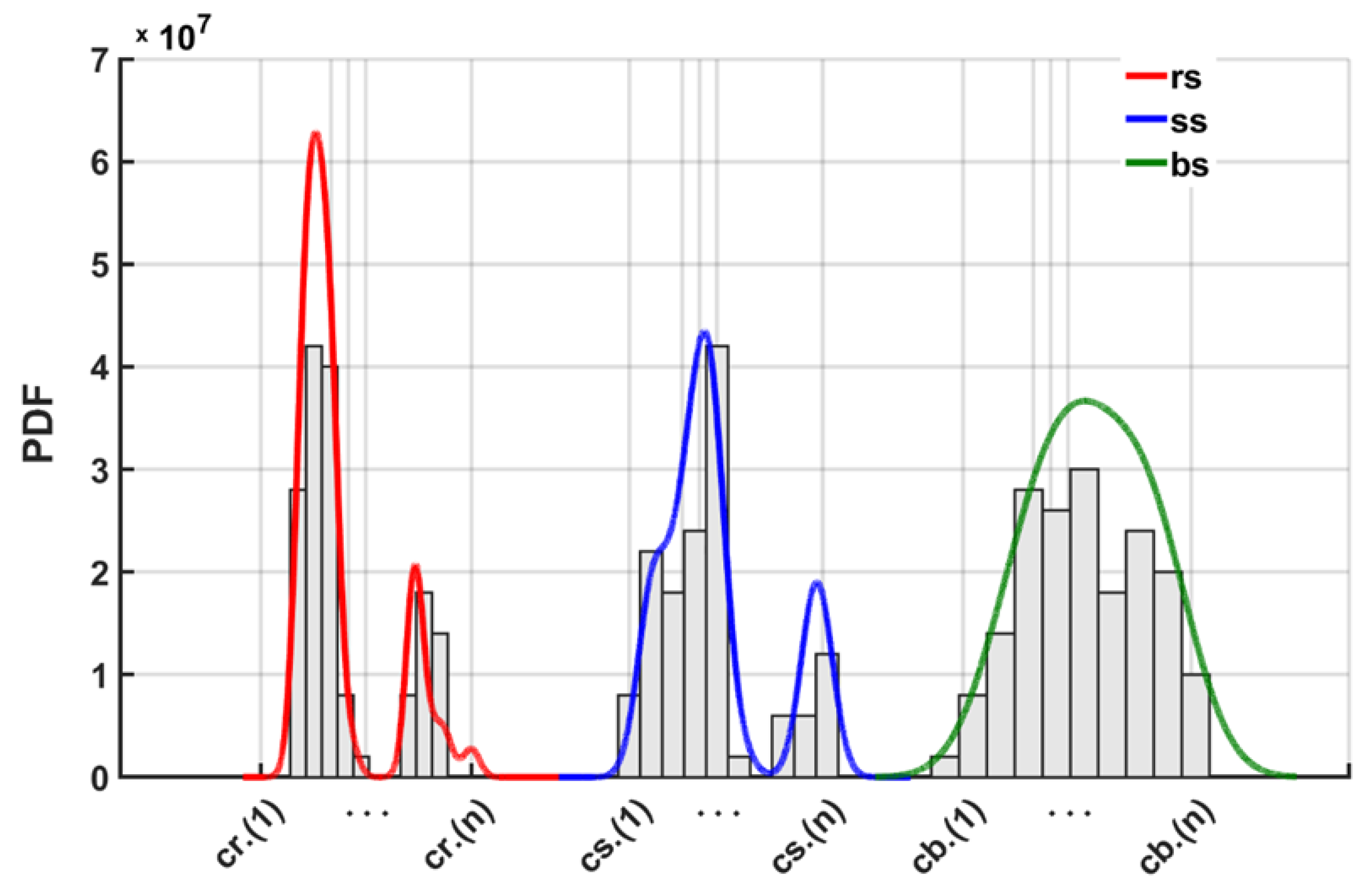
The Shewhart control chart capability to detect crack location is verified by comparing PDF coverage against crack growths for the three experimental samples (
Figure 8). Cracks with similar sizes will be grouped into logical ranges or bins. The predicted PDF curve outcomes show that the curve fit correlated well with the crack growth at different levels for surface and length cracks. Based on bin coverage shown in
Figure 8, the prediction accuracy varied between 93% to 97% for Cr, Cs and Cb respectively.
The crack information from irregular sensors gains access to the H-cluster algorithm for classification. The H-clustering algorithm discovered strongly related fractures at a local level to determine similarity (discussed in
Section 3.2). Following this, the algorithm provides an insight into the data by splitting the cracks into classes of cracks, such that cracks in a group are more identical to each other to cracks in other groups in terms of depth and length.
The number of clusters are unknown in advance by the algorithm which make it a suitable solution for partitioning our objects via a non-heuristic search [
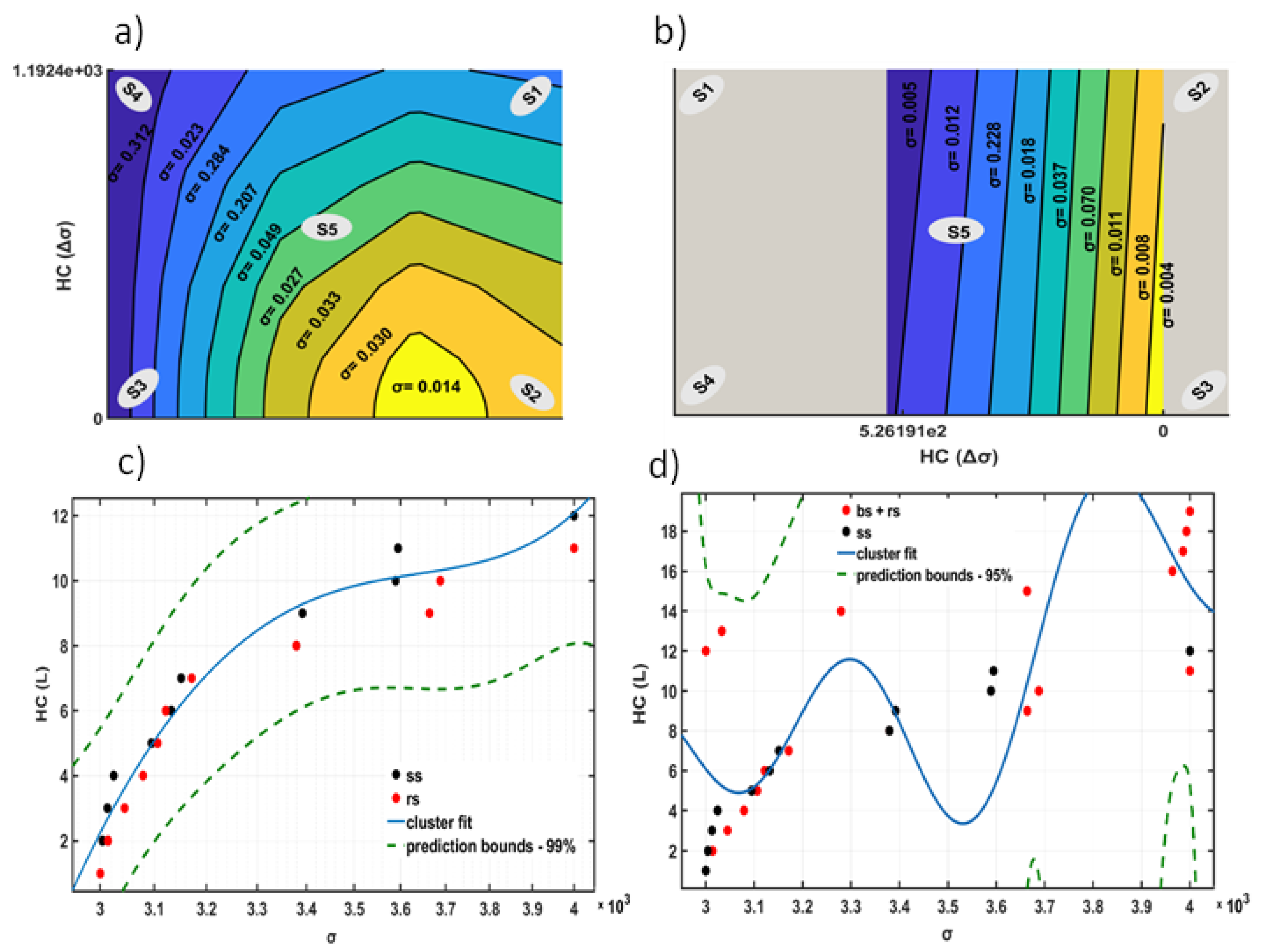
44]. As a result, the border of fractures could be evaluated as shown in
Figure 9a,b. As the height of the link increased with developing cracks, the measurement for HC algorithm was
L (
μ) that were originated from
σ. Therefore, the different
σ value shown in figure derived from
. The technique is applied successfully on a variety of dataset [
45,
46,
47,
48].
To verify the HC model prediction, a polynomial function from the order of two was adjusted to cluster links. For the model fit to ‘ss’, R² = %97 and the one fit to ‘bs+rs’ an R² = %91 can be achieved. The complete understanding of ‘bs’ behaviour is slightly complex as compared to ‘ss’ and ‘rs’ sets. It seems the cracks are propagated uneven and broad.
However, the different sizes of specimens and the shorter development of cracks could be calculated as potential reasons for the irregularity in the conduct of crack growth, which is beyond the scope of this study.
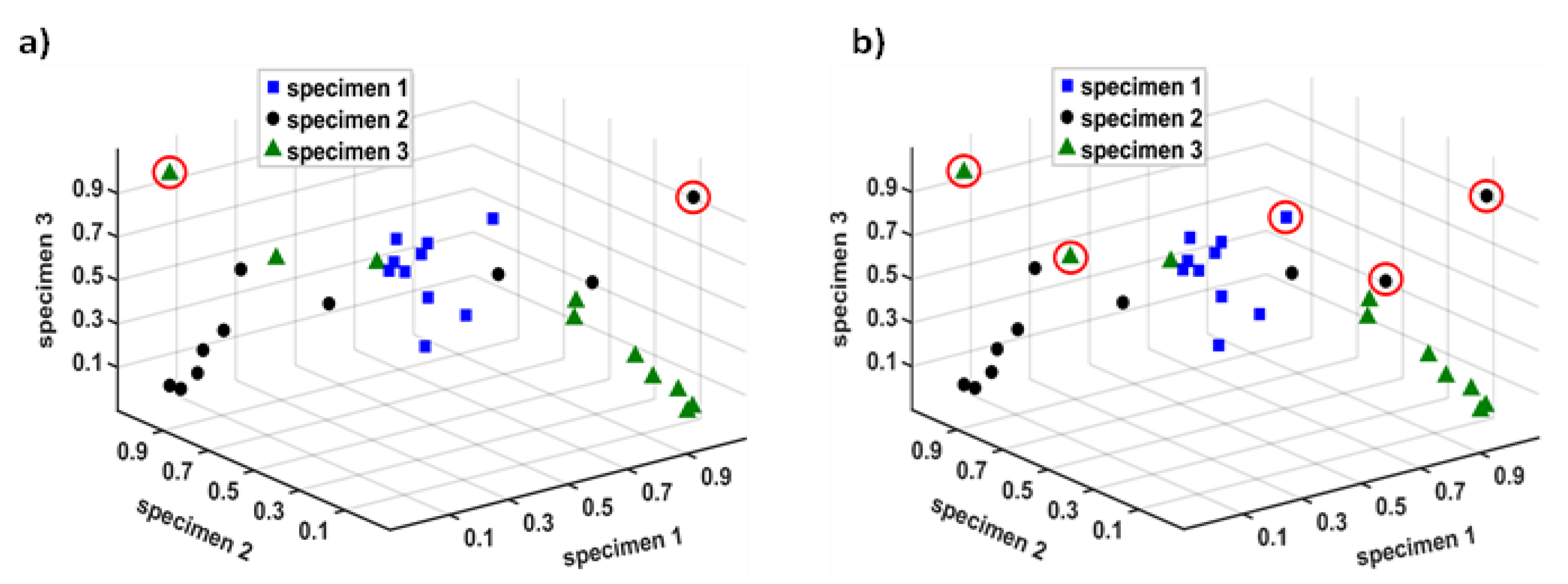
In terms of the Grubbs test and predicting deeper cracks, three sets of specimens with various levels of damage are compared. For a fair comparison, the same values of α = 0.5 and α = 10 that were discussed above are applied (
Figure 10). The G-test forms a probability that assumes samples belong to the core population, and any sample outside of this interval will be rejected by the test. The probability distribution will be based on the differences in sample means, where the boundary could be the sample’s standard deviation [
49].
5. Conclusions
In our study, we have developed a machine-learning framework for localising and classifying cracks, and identifying the final cracks. We used measured strain as the sole attribute for this framework. To collect strain data, we monitored three different types of specimens using a Bluetooth-based strain gauge sensor. Our experiments revealed that crack development causes the sensor output to deviate from its mean, and sensors with constant strain increments are closer to the fracture location. We utilised the Shewhart control chart to discover the crack location between the sensors. The use of this protocol demonstrated that sensors close to the fracture exhibit standard deviation violations from the lower and upper control limits. The effectiveness of the Shewhart control chart was confirmed using a probability density function curve with accuracy values exceeding 93%. Additionally, the hierarchical clustering algorithm was used to detect crack development through its connections. We then employed a polynomial function to evaluate hierarchical clustering patterns by interchanging samples from the three specimens, achieving prediction accuracies of over 91% for each model. This approach will enhance the speed and accuracy of material discovery. Furthermore, we applied a G-test to avoid encountering destructive fracture populations and predict fatigue cracks. With limited data available, we defined two thresholds to differentiate the confidence interval. Currently, our framework can indicate the increase in surface crack depth and length, but it lacks specificity in dimensions. In future work, we aim to enhance the system with more precise measurements to identify fracture length and depth.
Author Contributions
Conceptualization, G.L. and T.M.; methodology, G.L. and T.M.; validation, G.L. and T.M.; formal analysis, G.L. and T.M.; investigation, G.L. and T.M.; resources, X.X.; data curation, T.M..; writing—original draft preparation, T.M.; writing—review and editing, G.L. and T.M.; supervision, J.M. and D.F.; project administration, J.M. and D.F.; funding acquisition, J.M. and D.F. All authors have read and agreed to the published version of the manuscript.
Funding
This research was funded by the UK Research and Innovation’s Strength in Places Fund to the Belfast Maritime Consortium and led by Artemis Technologies.
Data Availability Statement
The data cannot be made publicly available upon publication because they are not available in a format that is sufficiently accessible by other researchers. The data that support the findings of this study are available upon reasonable request from the authors.
Conflicts of Interest
The authors declare no conflicts of interest.
References
- Chen, Hua-Peng, and Yi-Qing Ni. “Introduction to Structural Health Monitoring.” Structural Health Monitoring of Large Civil Engineering Structures, February 2, 2018, 1–14.
- Gisario, Annamaria, Mehrshad Mehrpouya, Atabak Rahimzadeh, Andrea De Bartolomeis, and Massimiliano Barletta. “Prediction Model for Determining the Optimum Operational Parameters in Laser Forming of Fiber Reinforced Composites.” Advances in Manufacturing 8, no. 2 (2020): 242–51.
- Legrain, Fleur, Jesús Carrete, Ambroise van Roekeghem, Stefano Curtarolo, and Natalio Mingo. “How Chemical Composition Alone Can Predict Vibrational Free Energies and Entropies of Solids.” Chemistry of Materials 29, no. 15 (2017): 6220–27.
- Raccuglia, Paul, Katherine C. Elbert, Philip D. Adler, Casey Falk, Malia B. Wenny, Aurelio Mollo, Matthias Zeller, Sorelle A. Friedler, Joshua Schrier, and Alexander J. Norquist. “Machine-Learning-Assisted Materials Discovery Using Failed Experiments.” Nature 533, no. 7601 (2016): 73–76.
- Kabbani, Mohammed S, and Hany A El Kadi. “Predicting the Effect of Cooling Rate on the Mechanical Properties of Glass Fiber–Polypropylene Composites Using Artificial Neural Networks.” Journal of Thermoplastic Composite Materials 32, no. 9 (2018): 1268–81.
- Liu, Xin, Federico Gasco, Johnathan Goodsell, and Wenbin Yu. “Initial Failure Strength Prediction of Woven Composites Using a New Yarn Failure Criterion Constructed by Deep Learning.” Composite Structures 230 (2019): 111505.
- Zhang, Shu Ling, Zhen Xiu Zhang, Zhen Xiang Xin, Kaushik Pal, and Jin Kuk Kim. “Prediction of Mechanical Properties of Polypropylene/Waste Ground Rubber Tire Powder Treated by Bitumen Composites via Uniform Design and Artificial Neural Networks.” Materials & Design 31, no. 4 (2010): 1900–1905.
- Davidson, Paul, and Anthony M. Waas. “Probabilistic Defect Analysis of Fiber Reinforced Composites Using Kriging and Support Vector Machine Based Surrogates.” Composite Structures 195 (2018): 186–98.
- Chapetti, M. “Fatigue Propagation Threshold of Short Cracks under Constant Amplitude Loading.”International Journal of Fatigue 25, no. 12 (December 2003): 1319–26.
- Chapetti, Mirco D., and Leandro F. Jaureguizahar. “Fatigue Behavior Prediction of Welded Joints by Using an Integrated Fracture Mechanics Approach.” International Journal of Fatigue 43 (October 2012): 43–53.
- Bang, D.J., A. Ince, and M. Noban. “Modeling Approach for a Unified Crack Growth Model in Short and Long Fatigue Crack Regimes.” International Journal of Fatigue 128 (November 2019): 105182.
- Bang, D.J., A. Ince, and L.Q. Tang. “A Modification of Unigrow 2-parameter Driving Force Model for Short Fatigue Crack Growth.” Fatigue & Fracture of Engineering Materials & Structures 42, no. 1 (June 19, 2018): 45–60.
- Newman, James C., and Balkrishna S. Annigeri. “Fatigue-Life Prediction Method Based on Small-Crack Theory in an Engine Material.” Journal of Engineering for Gas Turbines and Power 134, no. 3 (December 28, 2011).
- Lam, T.S., T.H. Topper, and F.A. Conle. “Derivation of Crack Closure and Crack Growth Rate Data from Effective-Strain Fatigue Life Data for Fracture Mechanics Fatigue Life Predictions.” International Journal of Fatigue 20, no. 10 (November 1998): 703–10.
- NOROOZI, A, G GLINKA, and S LAMBERT. “A Study of the Stress Ratio Effects on Fatigue Crack Growth Using the Unified Two-Parameter Fatigue Crack Growth Driving Force.” International Journal of Fatigue 29, no. 9–11 (September 2007): 1616–33.
- Santus, C., and D. Taylor. “Physically Short Crack Propagation in Metals during High Cycle Fatigue.” International Journal of Fatigue 31, no. 8–9 (August 2009): 1356–65.
- Perera, Yasith Sanura, Rajapaksha Mudiyanselage Muwanwella, Philip Roshan Fernando, Sandun Keerthichandra Fernando, and Thantirige Sanath Jayawardana. “Evolution of 3D Weaving and 3D Woven Fabric Structures.” Fashion and Textiles 8, no. 1 (March 5, 2021).
- Dai, D., and M. Fan. “Wood Fibres as Reinforcements in Natural Fibre Composites: Structure, Properties, Processing and Applications.” Natural Fibre Composites, 2014, 3–65.
- Rubino, Felice, Antonio Nisticò, Fausto Tucci, and Pierpaolo Carlone. “Marine Application of Fiber Reinforced Composites: A Review.” Journal of Marine Science and Engineering 8, no. 1 (January 6, 2020): 26.
- Manwell, James, Jon McGowan, and Anthony Rogers. Wind energy explained: Theory, design and Application. Chichester: Wiley, 2011.
- Muratoglu, Abdullah, and M. Ishak Yuce. Performance Analysis of Hydrokinetic Turbine Blade Sections 2 (2015): 1–10.
- Furst, Jonathan, Kaifei Chen, Hyung-Sin Kim, and Philippe Bonnet. “Evaluating Bluetooth Low Energy for IOT.” 2018 IEEE Workshop on Benchmarking Cyber-Physical Networks and Systems (CPSBench), April 2018.
- Vermaat, M. B., Roxana A. Ion, Ronald J. Does, and Chris A. Klaassen. “A Comparison of Shewhart Individuals Control Charts Based on Normal, Non-parametric, and Extreme-value Theory.” Quality and Reliability Engineering International 19, no. 4 (July 2003): 337–53.
- Roes, Kit C., and Ronald J. Does. “Shewhart-Type Charts in Nonstandard Situations.” Technometrics 37, no. 1 (February 1995): 15–24.
- Aslam, Muhammad. “Introducing Grubbs’s Test for Detecting Outliers under Neutrosophic Statistics – an Application to Medical Data.” Journal of King Saud University - Science 32, no. 6 (September 2020): 2696–2700.
- D. S. Young (2010), Book Reviews: „Statistical Tolerance Regions: Theory, Applications, and Computation”, TECHNOMETRICS, FEBRUARY 2010, VOL. 52, NO. 1, pp.143-144.
- Zhou, Chunguang, Changliang Zou, Yujuan Zhang, and Zhaojun Wang. “Nonparametric Control Chart Based o Change-Point Model.” Statistical Papers 50, no. 1 (2007): 13–28.
- Raji, Ishaq Adeyanju, Muhammad Hisyam Lee, Muhammad Riaz, Mu’azu Ramat Abujiya, and Nasir Abbas. “Outliers Detection Models in Shewhart Control Charts; an Application in Photolithography: A Semiconductor Manufacturing Industry.” Mathematics 8, no. 5 (2020): 857.
- Koutras, M.V., Bersimis, S. & Maravelakis, P.E. Statistical Process Control using Shewhart Control Charts with Supplementary Runs Rules. Methodol Comput Appl Probab 9, 207–224 (2007).
- Ryan, Thomas P. Statistical Methods for Quality Improvement. New York: J. Wiley and Sons, 2011.
- Albers, Willem, and Wilbert C.M. Kallenberg. “Estimation in Shewhart Control Charts: Effects and Corrections.” Metrika 59, no. 3 (June 1, 2004): 207–34.
- STEINER, STEFAN H., P. LEE GEYER, and GEORGE O. WESOLOWSKY. “Shewhart Control Charts to Detect Mean and Standard Deviation Shifts Based on Grouped Data.” Quality and Reliability Engineering International 12, no. 5 (1996): 345–53.
- Murtagh, Fionn, and Pedro Contreras. “Algorithms for Hierarchical Clustering: An Overview.” WIREs Data Mining and Knowledge Discovery 2, no. 1 (2011): 86–97.
- Nielsen, Frank. “Hierarchical Clustering.” Introduction to HPC with MPI for Data Science, 2016, 195–211.
- Murtagh, Fionn. “Hierarchical Clustering.” International Encyclopedia of Statistical Science, 2011, 633–35.
- Zhang, Tian, Raghu Ramakrishnan, and Miron Livny. “Birch.” Proceedings of the 1996 ACM SIGMOD international conference on Management of data - SIGMOD ’96, 1996.
- Zhu, Yunyun, Li Zhu, Yu Xiao, Minghu Zha, Tao Hu, and Mian Xiang. “Research on Hierarchical Clustering Leach Protocol Optimization Algorithm Based on Chebyshev Distance.” Journal of Physics: Conference Series 2456, no. 1 (March 1, 2023): 012040.
- Tibshirani, Robert, Guenther Walther, and Trevor Hastie. “Estimating the Number of Clusters in a Data Set via the Gap Statistic.” Journal of the Royal Statistical Society Series B: Statistical Methodology 63, no. 2 (July1, 2001): 411–23.
- Kachigan, Sam Kash. Statistical analysis: An interdisciplinary introduction to Univariate & Multivariate Methods. New York: Radius Press, 1986.
- Grubbs, Frank E. “Sample Criteria for Testing Outlying Observations.” The Annals of Mathematical Statistics 21, no. 1 (1950): 27–58.
- Stefansky, Wilhelmine. “Rejecting Outliers in Factorial Designs.” Technometrics 14, no. 2 (1972): 469–79.
- Cohn, T. A., J. F. England, C. E. Berenbrock, R. R. Mason, J. R. Stedinger, and J. R. Lamontagne. “A Generalized Grubbs-beck Test Statistic for Detecting Multiple Potentially Influential Low Outliers in Flood Series.” Water Resources Research 49, no. 8 (2013): 5047–58.
- Tsai, Tzong-Ru, Jyh-Jiuan Lin, Shuo-Jye Wu, and Hung-Chia Lin. “On Estimating Control Limits of X -Chart When the Number of Subgroups Is Small.” The International Journal of Advanced Manufacturing Technology 26, no. 11–12 (August 17, 2005): 1312–16.
- Blumenfeld, Dennis. Operations research calculations handbook, December 23, 2009.
- Fung, Benjamin C.M., Ke Wang, and Martin Ester. “Hierarchical Document Clustering Using Frequent Itemsets.” Proceedings of the 2003 SIAM International Conference on Data Mining, May 2003.
- Malik, Hassan, and John Kender. “High Quality, Efficient Hierarchical Document Clustering Using Closed Interesting Itemsets.” Sixth International Conference on Data Mining (ICDM’06), December 2006.
- Xiong, Hui, Michael Steinbach, Pang-Ning Tan, and Vipin Kumar. “HICAP: Hierarchical Clustering with Pattern Preservation.” Proceedings of the 2004 SIAM International Conference on Data Mining, April 22, 2004.
- Beil, Florian, Martin Ester, and Xiaowei Xu. “Frequent Term-Based Text Clustering.” Proceedings of the eighth ACM SIGKDD international conference on Knowledge discovery and data mining, July 23, 2002.
- Grubbs, Frank E. “Procedures for Detecting Outlying Observations in Samples.” Technometrics 11, no. 1 (February 1969): 1.
|
Disclaimer/Publisher’s Note: The statements, opinions and data contained in all publications are solely those of the individual author(s) and contributor(s) and not of MDPI and/or the editor(s). MDPI and/or the editor(s) disclaim responsibility for any injury to people or property resulting from any ideas, methods, instructions or products referred to in the content. |
© 2024 by the authors. Licensee MDPI, Basel, Switzerland. This article is an open access article distributed under the terms and conditions of the Creative Commons Attribution (CC BY) license (https://creativecommons.org/licenses/by/4.0/).
