
Submitted:
04 November 2024
Posted:
05 November 2024
You are already at the latest version
Abstract
Haug and Tatum [1, 2] have recently outlined a possible path to solving the Hubbletension within Rh = ct cosmology models using a trial-and-error algorithm for redshift scaling, 1 specifically z = (R_h/R_t) − 1 and z = (R_h/R_t)^{1/2}-1 . Their algorithm demonstrates that one canstart with the measured CMB temperature and a rough estimate of H_0. Based on this approach, they nearly perfectly match the entire distance ladder of observed supernovae by identifying a single value for H_0. However, their solution is based on a simple numerical search procedure, which, although it can be completed in a fraction of a second on a standard computer, is not a formal mathematical proof for resolving the Hubble tension.Here, we will demonstrate that the trial-and-error numerical method is not necessary and that the Hubble tension can be resolved using the same Haug and Tatum type R_h = ct model through a closed-form mathematical solution. Furthermore, we will prove that this solution is valid for a much more general case of any cosmological redshift scaling consistent with: z = (R)h/R)t)^x − 1. Haug and Tatum have only considered the most common assumptions of x = 1 and x = 1/2 .Our solution involves simply solving an equation to determine the correct value of H0. This is possible because an exact mathematical relation between H_0 and the CMB temperature has recently been established, in combination with the linearity in an R_h = ct model. We also demonstrate that a thermodynamic form of the Friedmann equation is consistent with a wide range of redshift scalings, namely: z = (R_h/R_t)^x − 1.
Keywords:
Hubble tension close dorm
; Hubble constant
; Cosmological redshift
; z
; CMB temperatur
1. Type Cosmological Models
The Haug and Tatum [1,2] cosmological model that we will discuss is unique in that it provides an exact mathematical relation between the CMB temperature, the Hubble constant and the cosmological red-shift. The Haug-Tatum cosmological model has developed over time in multiple stages. It is consistent with the principle, which describes a universe expanding at the speed of light without accelerated expansion. There are several -type cosmological models, and these models are still actively discussed in recent literature, see for example [3,4,5,6]. Melia [7] has recently demonstrated that cosmology seems more in line with recent observations from the James Webb Space Telescope than the -CDM model. The question of which cosmological model best fits different observed properties of the universe will undoubtedly be an ongoing discussion in the years to come. This paper offers additional evidence in favor of cosmology, as it seems that we with a closed-form mathematical solution can resolve the Hubble tension within such a cosmological model.
Standard cosmology is not able to predict the current CMB temperature, , despite it being one of the best-determined cosmological parameters, measured with extremely high precision. This limitation, for example, has been clearly pointed out in the review article by Narlikar and Padmanabhan [8]: “The present theory is, however, unable to predict the value of T at . It is therefore a free parameter in SC (Standard Cosmology).” Furthermore, they suggest that if one could link to other physical processes in the universe, this would: “clearly mark an improvement over the standard interpretation.”
In recent years, we have developed a new model based on Einstein’s general relativity theory that not only predicts with remarkable precision but also mathematically links to parameters such as . This advancement even appears to resolve the Hubble tension, a result we will demonstrate both mathematically and experimentally in this paper.
In 2015, Tatum et al. [9] heuristically presented the following formula for the Cosmic Microwave Background (CMB) temperature, which was later formally derived based on the Stefan-Boltzmann law [10,11] by Haug and Wojnow [12,13]:
where is the Boltzmann constant and is the Planck mass, is the Planck length [14,15], and is the Hubble radius and is the mass (equivalent) of the critical Friedmann [16] universe. The Stefan-Boltzmann law was developed basically for black bodies. The CMB temperature has been described as an almost perfect black body , see for example; Muller et al. [17] that states :
“Observations with the COBE satellite have demonstrated that the CMB corresponds to a nearly perfect black body characterized by a temperature at , which is measured with very high accuracy, ."
Equation (1) has also recently been derived using a geometric mean approach, see [18]. Additionally, Haug and Tatum [1] have demonstrated that to be consistent with the observed relation , see [19,20,21], the predicted redshift seems like it must be given by:
However, they also show that one can have the more common scaling, but that this leads to , which does not seem to be supported by observational studies. However, we have to be careful here, as even in observational studies, there are often assumptions or hidden assumptions that one must carefully revisit before prematurely concluding one way or the other. In this paper, we will demonstrate that in a more general model with cosmological redshift scaling of the form:
where x is what we can call the scaling factor. The x is decided by assumption based on observations and logic, for example if one decide the cosmological scaling should be (a scaling used in multiple models such as the Melia model) one simply set or if one want scaling one set , but one can also set x to any other value and still one will by solving an equation we soon will look at get the one and the same value for that seems to solves the Hubble tension. Technically one could even make x time dependent .
It is important to be aware we only claim to solve the Hubble tension inside a class of cosmological models this way and not at all inside the -CDM model.
For example in the Melia model has a cosmological redshift corresponding to in our suggested general redshift scaling formula. Melia has however no equation for the relation between the CMB temperature now and . Haug and Tatum model B in [1] given above correspond then to , the Haug and Tatum model A [1] that has the same redshift scaling as the Melia model correspond to , but this model is still different than the Melia model as we in this have a tight mathematical relation between CMB temperature and that Melia not have in his model.
For the general red-shift scaling equation (3) to be consistent with the CMB temperature formula derived from the Stefan-Boltzmann law we get the following relation for the CMB temperature now and in past cosmological epochs:
Observations seems to favor a , even if the exact value of x not yet is experimentally fully settled. We will not in this paper conclude on the optimal scaling factor x, but leave it up to further research to find the optimal x. The important point in this paper is that the Hubble tension itself seems to be solved for any scaling factor x in the closed form solution we soon will present.
Haug and Tatum demonstrate that the predicted redshift in one of their two models models must satisfy:
be aware they do similar for red-shift scaling.
They then use a smart trial-and-error algorithm, such as the Newton-Raphson method or the bisection method, to find the value of that minimizes the sum of the prediction errors . They demonstrate that this approach leads to a single value that perfectly matches the model with the full observed distance ladder, something that seems to solve the Hubble tension.
However, here we simply solve equation (5) for , which yields:
In the case where the predicted redshift is exactly equal to the observed redshift , we must have . Substituting back into Equation (9) gives:
The last part, the Latin upsilon: , is a composite constant made up of well-known constants (which we [22,26] have coined ). This is the same formula as given by [22], but here we have just demonstrated that this formula is strictly valid only when the predicted redshift exactly matches the observed redshift, or as we soon will see we can use Equation (9) to match the full distance ladder of observed supernova redshifts by simply finding this one value directly from the current measured CMB temperature.
This means that we only need to know and this constant to closely match all observed cosmological redshifts. The reason we say “close to perfect" rather than "perfect" is due to small measurement errors in both the measured CMB temperature and in G, and that is the only uncertainty in this method. The Boltzmann constant, the speed of light, and the reduced Planck constant have no uncertainty, as they have been exactly defined since the 2019 NIST CODATA standard.
We can generalize this to any redshift scaling assumption inside cosmology as long as we assume the equation (1) that has been derived from the Stefan-Boltzmann law is correct, we then get:
Solved for we get:
when we have (or want) perfect prediction of redshift we must have and then we end up with and therefore we must have:
That is for any scaling factor x one get exactly the same dependent on only the CMB temperature measured now, the Boltzmann constant, the Planck length, the speed of light and the Planck constant. The only variable is the CMB temperature that has been measured very precisely.
2. Distance, Hubble Constant and Redshift
If we solve the general redshift formula for we get:
This means the predicted distance to the observed redshift must be:
further if we solve this for we get:
Here will be the estimated distance to the object emitting the photons. For very low redshift we have and we can use the first term of the Taylor expansion to get:
and now solved for z we get:
In the case , this is identical to the standard -CDM cosmological redshift prediction formula approximation when used for . Haug and Tatum examine both the special case of , where one obtains the standard distance formula when , and a model corresponding to , which predicts twice the distance of -CDM for low z. However, as we will soon demonstrate, any value of x can be used in the redshift scaling and still resolve the Hubble tension. The choice of x therefore depends on other observations beyond predictions of the Hubble constant versus redshift. It is influenced by factors such as determining the optimal in in comparison with observed data; see, for example, [23], which suggests that should be close to 0. However, it is crucial to carefully examine the assumptions and methods used in any observational study to arrive at its results.
Nevertheless, this is not the primary focus of this paper. The main discussion, as we will see in the next section, is that within the cosmology model presented here, any choice of x can be used while still allowing us to match all observed SN Ia redshifts with a single value. Most values of x, and likely all except one, should be ruled out based on other types of observations, such as the observed scaling.
In the -CDM model, at least three different distances are considered for a given cosmological redshift: the comoving distance, the angular diameter distance, and the luminosity distance. These three distances differ from each other in the -CDM model, which is fully consistent within the model and necessarily accounts for phenomena such as accelerated expansion. In cosmological models, however, there is no accelerated expansion, and in the Haug-Tatum cosmological model (), the comoving, luminosity, and angular diameter distances are identical, see [24] for in detailed discussion on this point. We believe this is not a coincidence. Only the redshift scaling is consistent with , and it is the only redshift scaling where the three distances—comoving, luminosity distance, and angular diameter distance—are identical. For any other x, the three distances are not the same.
Importantly, is also consistent with the well-known Etherington equation [25], which is based on purely geometrical principles linked to general relativity. Both the -CDM model and the model used here are consistent with the Etherington equation: , where is the luminosity distance and is the angular diameter distance. In the next section, we will see how our model can match one of the largest databases of supernovae of type SN Ia while simultaneously predicting their distances. We suspect that the -CDM model has become overly complex due to its three different distances for each observed . In cosmology, things appear to be much simpler, and we are even able to match all the SN Ia with a single parameter value, as we will explore next. The distance to cosmological redshifts is not the main topic of this article.
3. Predictions Relative to the Observations Using the Full Distance Ladder from the PantheonPlus Compilation
Here, we will see if our model can match all the observed cosmological redshifts by simply determining the constant from Equation (10). However to demonstrate the superiority of Equation (10), we will first instead use the predicted value for by for example Riess et al. [27] of km/s/Mpc. We plot the Riess et al. value, accounting for 2 standard deviations (STD), and from this, we get Figure 1. The blue line represents the predicted redshift from km/s/Mpc, while the green lines represent the 2 STD confidence interval, i.e., km/s/Mpc. We can see that even the 95% confidence interval falls outside the observations, meaning that any value within this interval does not come close to matching the observed redshifts in our cosmological model.
Figure 2 demonstrates the results we get when we instead calculate based on Equation (7) when using the Dhal et al [28] measured CMB value of . According to our theory, this should provide a perfect match between the observed and predicted values, and as we can see, the observed and predicted values lie on top of each other. The confidence interval is now so narrow that even if we plotted it, it would appear to overlap with the observed values. The predicted when using this measured CMB temperature.
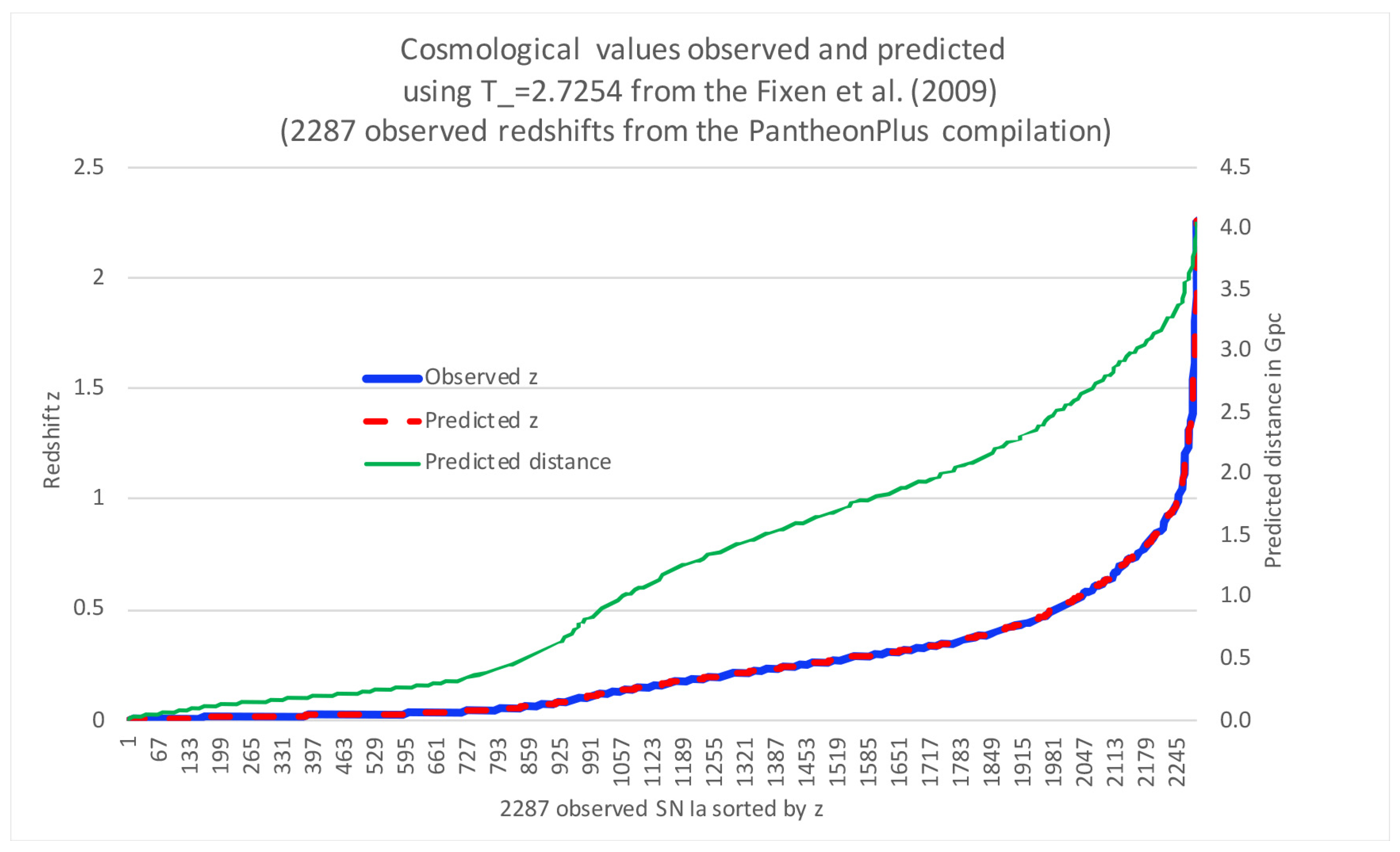
Figure 3 demonstrate the results we get when we calculate based on Equation (10) when the measured CMB value of Fixsen [29]: , this lead to a basically perfect match between predicted and observed SN Ia redshifts with a predicted
It is important to understand that the results in this section is independent on the value selected for the scaling factor x in in our cosmology.
4. The new Thermodynamic Friedmann Equation Consistent with the General Red-Shift Scaling of the form
Haug and Tatum [30] have recently demonstrated that the critical Friedmann [16] equation:
can be rewritten in thermodynamical form:
Keep in mind if doing the caculations that , something we get by simply solving the Planck length formula , see also [31].
Here we will generalize this to
and when this will simply reduce to (17). We have simply replaced with . However when we end up getting equation (17) which demonstrate the thermodynamic form of the Haug and Tatum equation is very general and robust, it is valid for a wide range of redshift scaling choices (the choice off x) inside cosmology.
From the sections above, it is clear that this thermodynamic Friedmann equation is valid and identical x scaling factors in , as they all lead to the exactly the same .
More importantly, the thermodynamic Friedmann equation, when carefully studied in relation to our empirical and theoretical work, clearly seems to present a solution to the Hubble tension. However, further discussions and testing by many other researchers are needed before a consensus can be reached. We hope the research community is open-minded enough to carefully consider this possibility and not simply ignore it due to biases based on the current consensus model, where the Hubble tension has yet to be solved.
5. Conclusions
Haug and Tatum have outlined a way to solve the Hubble tension inside cosmology based on new exact relations between the CMB temperature the Hubble constant and redshift, they however use a numerical search algorithm to do so and have only considered and cosmological redshift scaling. Even if their method is intuitive and powerful we here demonstrate one can simply solve one of their equations and further based on logic get to the one single value that make their model matching all observed SN Ia. In other words this leads to a closed form solution of the Hubble tension inside cosmology. We get a when relying on the very precise Dhal et al measured CMB value matching leading to matching all the observed SN Ia redshifts across the full distance ladder in the PantheonPlusSH0ES compilation. This is the same value Haug and Tatum got from their numerical search algorithm solution when solving the Hubble tension. It is basically the same solution, one is using numerical search algorithm while the later used closed form solution. The closed form solution is naturally more elegant as no numerical search rutine with many calculations are needed to find the that matches all the supernovas. Further the solution in this paper is generalized for cosmological scaling, while Haug and Tatum only have considered the case equivalent to and .
So it looks like we have a path to solving the Hubble tension in cosmology, but this does not solve the Hubble tension inside -CDM cosmology. Further investigation between cosmology and -CDM cosmology is therefore warranted.
Data Availability Statement
The supernova PantheonPlusSH0ES database that we have used can be found here: https://github.com/PantheonPlusSH0ES/DataRelease/blob/main/Pantheon%2B_Data/1_DATA/all_redshifts_PVs.csv
Conflicts of Interest
The authors declare no conflict of interest.
References
- E. G. Haug and E. T. Tatum. Solving the Hubble tension using the union2 supernova database. Preprints.org 2024. [CrossRef]
- E. G. Haug and E. T. Tatum. Planck length from cosmological redshifts solves the Hubble tension. ResearchGate.org 2024. [CrossRef]
- F. Melia. A comparison of the Rh=ct and ΛCDM cosmologies using the cosmic distance duality relation. Monthly Notices of the Royal Astronomical Society. [CrossRef]
- M. V. John. Rh=ct and the eternal coasting cosmological model. Monthly Notices of the Royal Astronomical Society 2019, 484. [CrossRef]
- F. Melia. Thermodynamics of the Rh=ct universe: a simplification of cosmic entropye. European Journal of Physics C 2021, 81, 234. [CrossRef]
- F. Melia. Model selection with baryonic acoustic oscillations in the lyman-α forest. European Physics Letters 2023, 143, 59004. [CrossRef]
- F. Melia. Strong observational support for the rh=ct timeline in the early universe. Physics of the Dark Universe 2024, 46, 101587. [CrossRef]
- J. V. Narlikar and T. Padmanabhan. Standard cosmology and alternatives: A critical appraisal. Annual Review of Astronomy and Astrophysics 1979, 39, 211. [CrossRef]
- E. T. Tatum, U. V. S. E. T. Tatum, U. V. S. Seshavatharam, and S. Lakshminarayana. The basics of flat space cosmology. International Journal of Astronomy and Astrophysics 2015, 5, 116. [Google Scholar] [CrossRef]
- Stefan, J. Über die beziehung zwischen der wärmestrahlung und der temperatur. Sitzungsberichte der Mathematisch-Naturwissenschaftlichen Classe der Kaiserlichen Akademie der Wissenschaften in Wien 1879, 79, 391. [Google Scholar]
- L. Boltzmann. Ableitung des stefanschen gesetzes, betreffend die abhängigkeit der wärmestrahlung von der temperatur aus der electromagnetischen lichttheori. Annalen der Physik und Chemie 1879, 22, 291.
- E. G. Haug. CMB, Hawking, Planck, and Hubble scale relations consistent with recent quantization of general relativity theory. International Journal of Theoretical Physics, Nature-Springer 2024, 63. [CrossRef]
- E. G. Haug and S. Wojnow. How to predict the temperature of the CMB directly using the Hubble parameter and the Planck scale using the Stefan-Boltzman law. Research Square, Pre-print, accepted and forthcoming JAMP 2023. [CrossRef]
- M. Planck. In Natuerliche Masseinheiten; Der Königlich Preussischen Akademie Der Wissenschaften: Berlin, Germany, 1899; Available online: https://www.biodiversitylibrary.org/item/93034#page/7/mode/1up.
- M. Planck. Vorlesungen über die Theorie der Wärmestrahlung. Leipzig: J.A. Barth, p. 163, see also the English translation “The Theory of Radiation" (1959) Dover, 1906.
- A. Friedmann. Über die krüng des raumes. Zeitschrift für Physik 1922, 10, 377. [CrossRef]
- S. et. al Muller. A precise and accurate determination of the cosmic microwave background temperature at z=0.89. Astronomy & Astrophysics 2013, 551. [CrossRef]
- E. G. Haug and E. T. Tatum. The Hawking Hubble temperature as a minimum temperature, the Planck temperature as a maximum temperature and the CMB temperature as their geometric mean temperature. Journal of Applied Physics and Mathematics (accepted and forthcoming), 2024c.
- I. de Martino and et. al. Measuring the redshift dependence of the cosmic microwave background monopole temperature with planck data. The Astrophysical Journal 2012, 757, 144. Available online: https://iopscience.iop.org/article/10.1088/0004-637X/757/2/144. [CrossRef]
- L. Yunyang. Constraining cosmic microwave background temperature evolution with sunyaev–zel’dovich galaxy clusters from the atacama cosmology telescope. The Astrophysical Journal 2021, 922, 136. [CrossRef]
- D.A. Riechers, A. D.A. Riechers, A. Weiss, and F. et al. Walter. Microwave background temperature at a redshift of 6.34 from H2O absorption. Nature 2022, 58, 602. [Google Scholar] [CrossRef]
- E. T. Tatum, E. G. E. T. Tatum, E. G. Haug, and S. Wojnow. High precision Hubble constant determinations based upon a new theoretical relationship between CMB temperature and H0. Journal of Modern Physics 2024, 15, 1708. [Google Scholar] [CrossRef]
- P. Noterdaeme, P. P. Noterdaeme, P. Petitjean, R. Srianand, C . Ledoux, and S. López. The evolution of the cosmic microwave background temperature. Astronomy and Astrophysics 2011, 526. [Google Scholar] [CrossRef]
- E. G. Haug. The CMB luminosity distance and cosmological redshifts. Journal of Applied Mathematics and Physics 2024, 12, 3496. [CrossRef]
- I.M.H. Etherington. Lx. on the definition of distance in general relativity. The London, Edinburgh, and Dublin Philosophical Magazine and Journal of Science 1933, 15, 761. [CrossRef]
- E. T. Tatum. Upsilon constants and their usefulness in Planck scale quantum cosmology. Journal of Modern Physics 2024, 15, 167. [CrossRef]
- A. G. Riess and et. al. A comprehensive measurement of the local value of the Hubble constant with 1 km s-1 Mpc-1 uncertainty from the Hubble space telescope and the sh0es team. The Astrophysical Journal 2021, 934. [CrossRef]
- Dhal, S.; Singh, S.; Konar, K.; Paul, R.K. Calculation of Cosmic Microwave Background radiation parameters using COBE/FIRAS dataset. Experimental Astronomy (2023) 2023, 612, 86. [Google Scholar] [CrossRef]
- Fixsen, D.J. The Temperature of the Cosmic Microwave Background. The Astrophysical Journal 2009, 707, 916. [Google Scholar] [CrossRef]
- E. G. Haug and E. T. Tatum. Friedmann type equations in thermodynamic form lead to much tighter constraints on the critical density of the universe. 2024. Available online: https://www.preprints.org/manuscript/202403.1241/v2.
- E. G. Haug. Progress in the composite view of the newton gravitational constant and its link to the planck scale. Universe 2022, 8. [CrossRef]
Figure 1.
This figure shows observed redshift values from 2287 type Ia supernovae from PantheonPlusSH0ES, sorted by redshift (blue line). Based on the measured CMB temperature by Dhal et al. (2023) of , the blue line represents our predictions based on , and the green lines represent the 2 STD confidence interval . We find that the Riess et al. value cannot match the observed redshifts in this model.
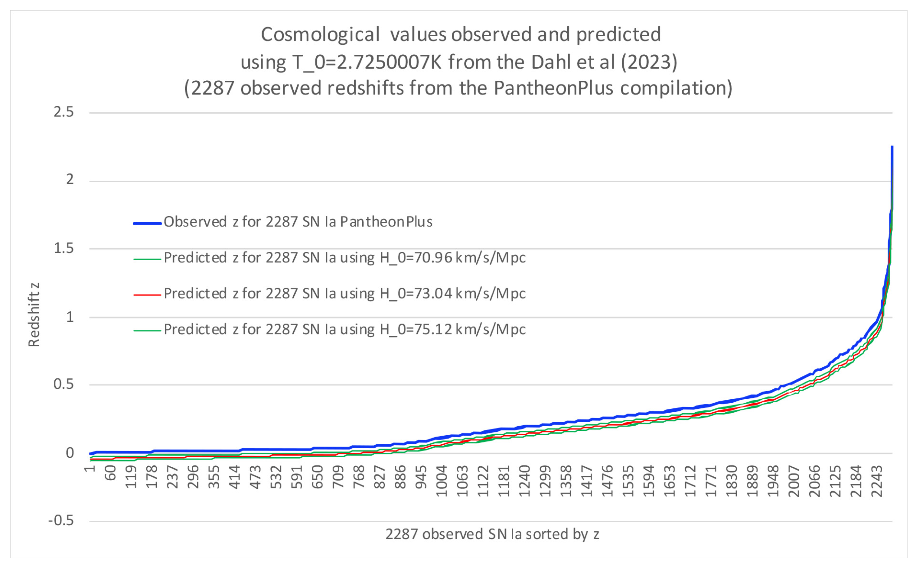
Figure 2.
This figure shows observed redshift values from 2287 type Ia supernovae, sorted by redshift (blue line). Based upon the measured CMB temperature by Dhal et al (2023) of , the red line represents our predictions based on , which we extracted from the data using equation (7).
Figure 2.
This figure shows observed redshift values from 2287 type Ia supernovae, sorted by redshift (blue line). Based upon the measured CMB temperature by Dhal et al (2023) of , the red line represents our predictions based on , which we extracted from the data using equation (7).
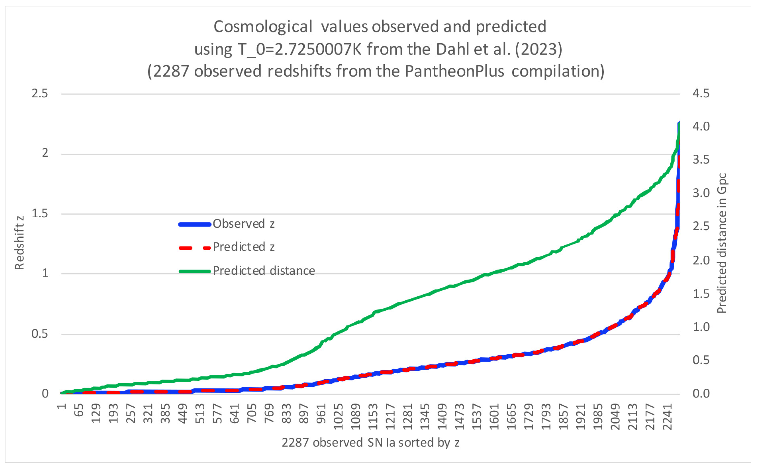
Figure 3.
This figure shows observed redshift values from 2287 type Ia supernovae, sorted by redshift (blue line). Based upon the measured CMB temperature by Fixen et al (2009) of , the red line represents our predictions based on calculated from equation (7).
Figure 3.
This figure shows observed redshift values from 2287 type Ia supernovae, sorted by redshift (blue line). Based upon the measured CMB temperature by Fixen et al (2009) of , the red line represents our predictions based on calculated from equation (7).
Disclaimer/Publisher’s Note: The statements, opinions and data contained in all publications are solely those of the individual author(s) and contributor(s) and not of MDPI and/or the editor(s). MDPI and/or the editor(s) disclaim responsibility for any injury to people or property resulting from any ideas, methods, instructions or products referred to in the content. |
© 2024 by the author. Licensee MDPI, Basel, Switzerland. This article is an open access article distributed under the terms and conditions of the Creative Commons Attribution (CC BY) license (http://creativecommons.org/licenses/by/4.0/).
Copyright: This open access article is published under a Creative Commons CC BY 4.0 license, which permit the free download, distribution, and reuse, provided that the author and preprint are cited in any reuse.


