Chaotic Dynamics, Sequence Density, and Chaos Suppression: A Study in Euclidean and Riemannian Spaces Inspired by Collatz-like Problems

Preprint

Article

Chaotic Dynamics, Sequence Density, and Chaos Suppression: A Study in Euclidean and Riemannian Spaces Inspired by Collatz-like Problems

Altmetrics

Downloads

Views

Comments

Rafik zeraoulia^*

This version is not peer-reviewed

Submitted:

21 September 2024

Posted:

24 September 2024

You are already at the latest version

Alerts

Abstract

In this paper, we explore the surprising behavior of certain discrete maps, drawing inspiration from Collatz-like problems and advanced techniques in analytic number theory, dynamical systems, and differential geometry. Specifically, we investigate a driven cubic-quintic Duffing equation and predict the number of limit cycles around equilibrium points. Furthermore, we develop a novel theoretical framework for chaos suppression in damped-driven systems, leveraging sequences derived from Collatz-like problems. Our study also focuses on analyzing the density of these sequences in both Euclidean and Riemannian metric spaces, providing a comparative analysis of their distribution properties. We estimate the growth rate of sequence density analytically and numerically, highlighting the sensitivity of the density values to the choice of parameters in both metric spaces. Our results present new insights into the behavior of these sequences and their implications for number theory, chaotic dynamics, and geometric analysis.

Keywords:

Subject: Computer Science and Mathematics - Computational Mathematics

1. Main Result

1) A number m has no predecessor if the interval $[m \sqrt{2}, (m + 1) \sqrt{2}]$ contains no even numbers and the interval $[m / \sqrt{2}, (m + 1) / \sqrt{2}]$ contains no odd numbers. The number of such values $m < 10^{ℓ}$ for $ℓ = 1, 2, 3, 4, 5, 6$ is $r_{ℓ} = 2, 29, 292, 2928, 29289, 292893$ . Curiously, for $ℓ \leq 6$ , the number $r_{ℓ}$ is approximately equal to $10^{ℓ} / \sqrt{2} .$
2) A simple algorithm for computing these values involves calculating the sum of all values of m for which either interval contains an even or odd number.
3) However, some inconsistencies remain, prompting the need for a better algorithm. See Figure 6.
4) Our result shows that the sequence exhibits higher and more localized density in Euclidean metric space compared to Riemannian space, where density is more sensitive to the parameter $α$ . As $ϵ \to 0$ in Euclidean space, the density experiences rapid growth, indicating a highly clustered distribution of sequence points.

2. Introduction

The Collatz conjecture is one of the most famous unsolved problems in mathematics [7,13]. The conjecture asks whether repeating two simple arithmetic operations will eventually transform every positive integer into 1. Specifically, each term in the sequence is derived by applying the following rules: if the previous term is even, the next term is half of it; if the previous term is odd, the next term is three times the previous term plus one. The conjecture asserts that every sequence, regardless of the starting integer, eventually reaches 1. Remarkably, this has been computationally tested for numbers up to approximately

5.48 \cdot 10^{18}

, a substantial achievement given the progress in computational capabilities over the past five decades.

Recent advancements in meta-mathematics and integer theory have led to the formalization of new theoretical number systems, potentially opening the door to novel analytical frameworks [18]. A particularly intriguing avenue involves the Collatz conjecture and similar discrete map problems, where sequences generated by iterative arithmetic operations provide a rich structure for exploration [15]. Such frameworks, including those emerging from the 3x+1 problem [17], have demonstrated considerable utility in mining and extracting knowledge about various conjectures and theorems in number theory, including those related to transcendental numbers such as

π

and

\sqrt{2}

[16,17].

The study of discrete dynamical systems, especially those related to Collatz-like problems, has garnered significant attention in recent years. Much of the research has focused on understanding the boundedness, periodicity, and divergence of sequences derived from these problems [1,3,4,5,14]. In this paper, we extend this study by focusing on a family of borderline Collatz-like problems, defined as maps that behave similarly to the original conjecture but with slight modifications. One particular case involves the map

f_{α} (n) = \{\begin{matrix} ⌊n α⌋ & if n even, \\ ⌊n / α⌋ & if n odd, \end{matrix}

for

α > 0

[10]. This map generates sequences that exhibit surprising behavior when

α = \sqrt{2}

, revealing connections between discrete dynamics, irrationality measures, and parity-related phenomena. [24]

In addition to the traditional analytical tools used in the study of discrete dynamical systems, we propose a geometric approach by incorporating Ricci flow and Riemannian metrics. Ricci flow, a powerful tool from differential geometry, describes the evolution of a Riemannian metric in a way that smooths out irregularities in curvature over time. By applying Ricci flow to the geometric representation of discrete maps, we can investigate how the curvature of the underlying manifold influences the behavior of these sequences, particularly in terms of convergence, divergence, and periodicity.

The use of Riemannian metrics allows us to introduce a more structured geometric perspective on the discrete systems under study. By embedding the sequences generated by the Collatz-like maps into a Riemannian manifold, we can analyze their evolution in a continuous geometric space. The Ricci flow then serves as a means of tracking how the system’s geometry deforms over time, potentially revealing new symmetries and invariant properties of the sequences.

This geometric approach offers a novel framework for studying chaotic behavior in discrete systems. Specifically, we show that by applying Ricci flow to certain borderline Collatz-like maps, we can smooth out chaotic regions and suppress chaotic dynamics in systems such as the driven cubic-quintic Duffing equation. This opens new pathways for chaos control and stabilization in dynamical systems through geometric methods, complementing existing analytic approaches.

Thus, our study contributes both new results regarding the behavior of Collatz-like sequences and a geometric framework that leverages Ricci flow and Riemannian metrics to deepen our understanding of chaos suppression in discrete and continuous systems. We believe this interdisciplinary approach, combining tools from number theory, dynamical systems, and differential geometry, will offer significant insights into longstanding problems in these fields.

3. Analysis and Discussion

We define the following mapping:

f : n \mapsto \{\begin{matrix} ⌊n / \sqrt{2}⌋ & if n is even, \\ ⌊n \sqrt{2}⌋ & if n is odd . \end{matrix}

Let

f^{\circ (r + 1)} : = f \circ f^{\circ r}

, and consider the orbit of

n = 73

under repeated iterations of f, which produces the sequence

f^{\circ r} (73)

73, 103, 145, 205, 289, 408, 288, 203, 287, 405, 572, 404, 285, 403, 569, 804, 568, 401, \dots

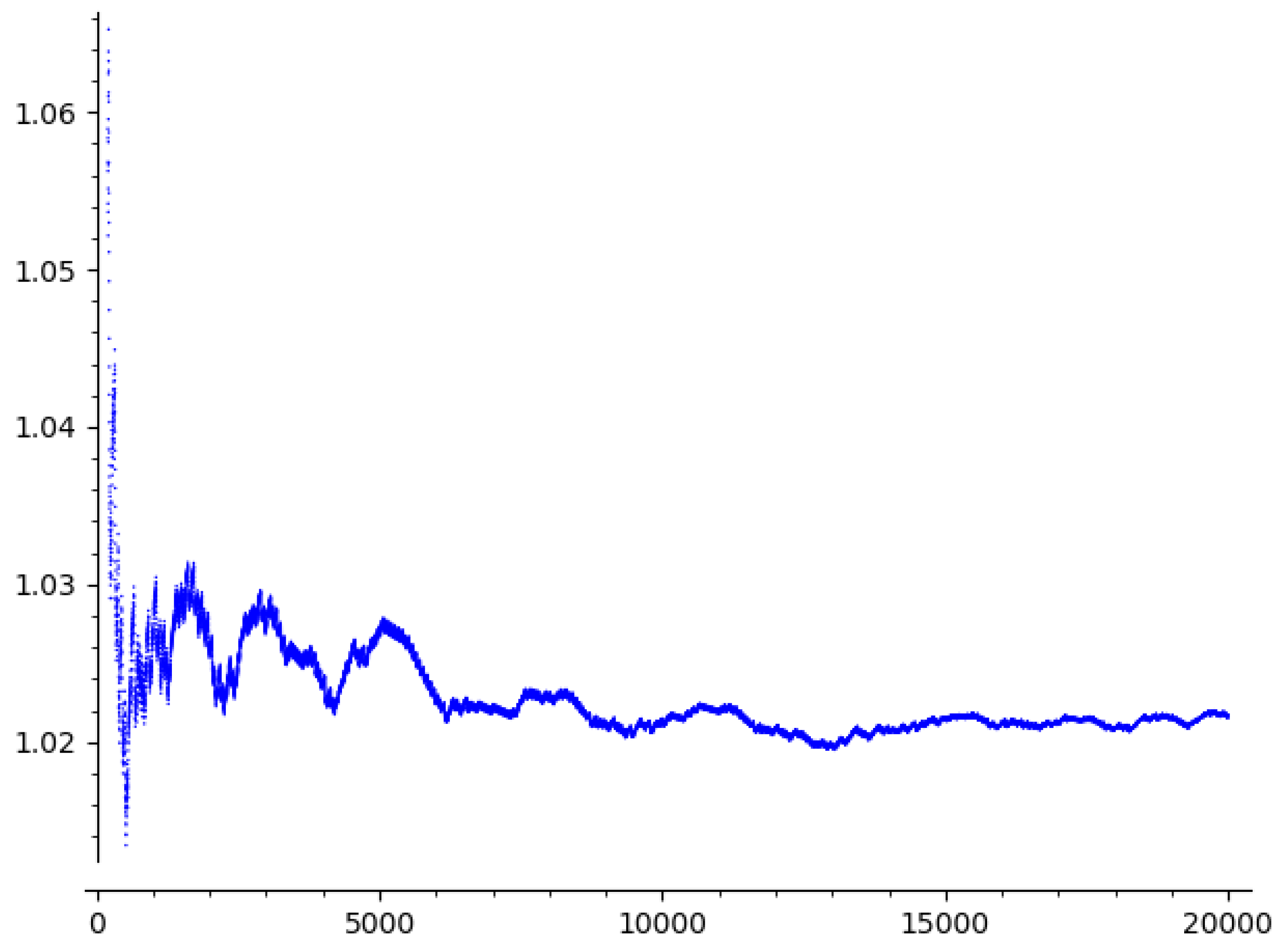
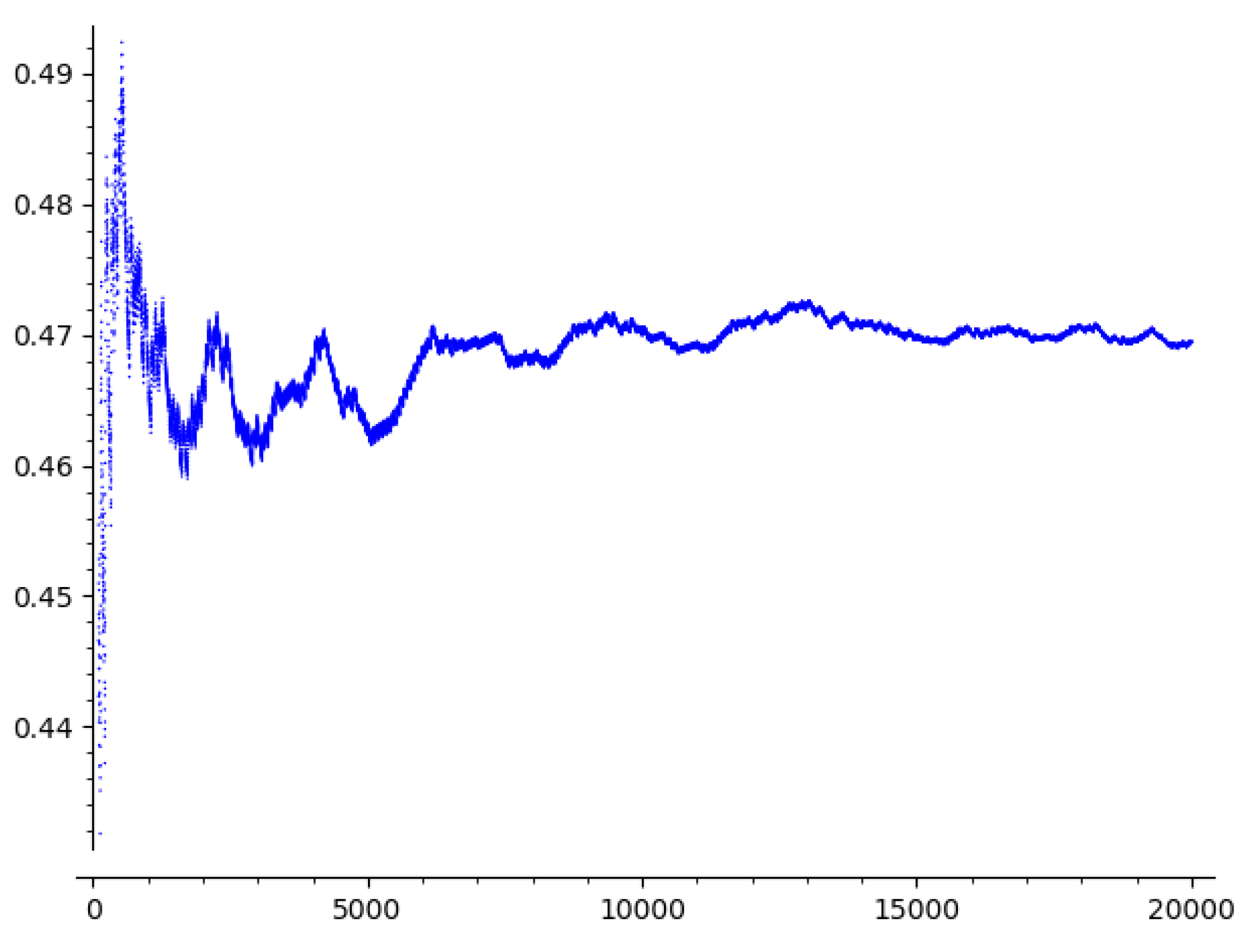
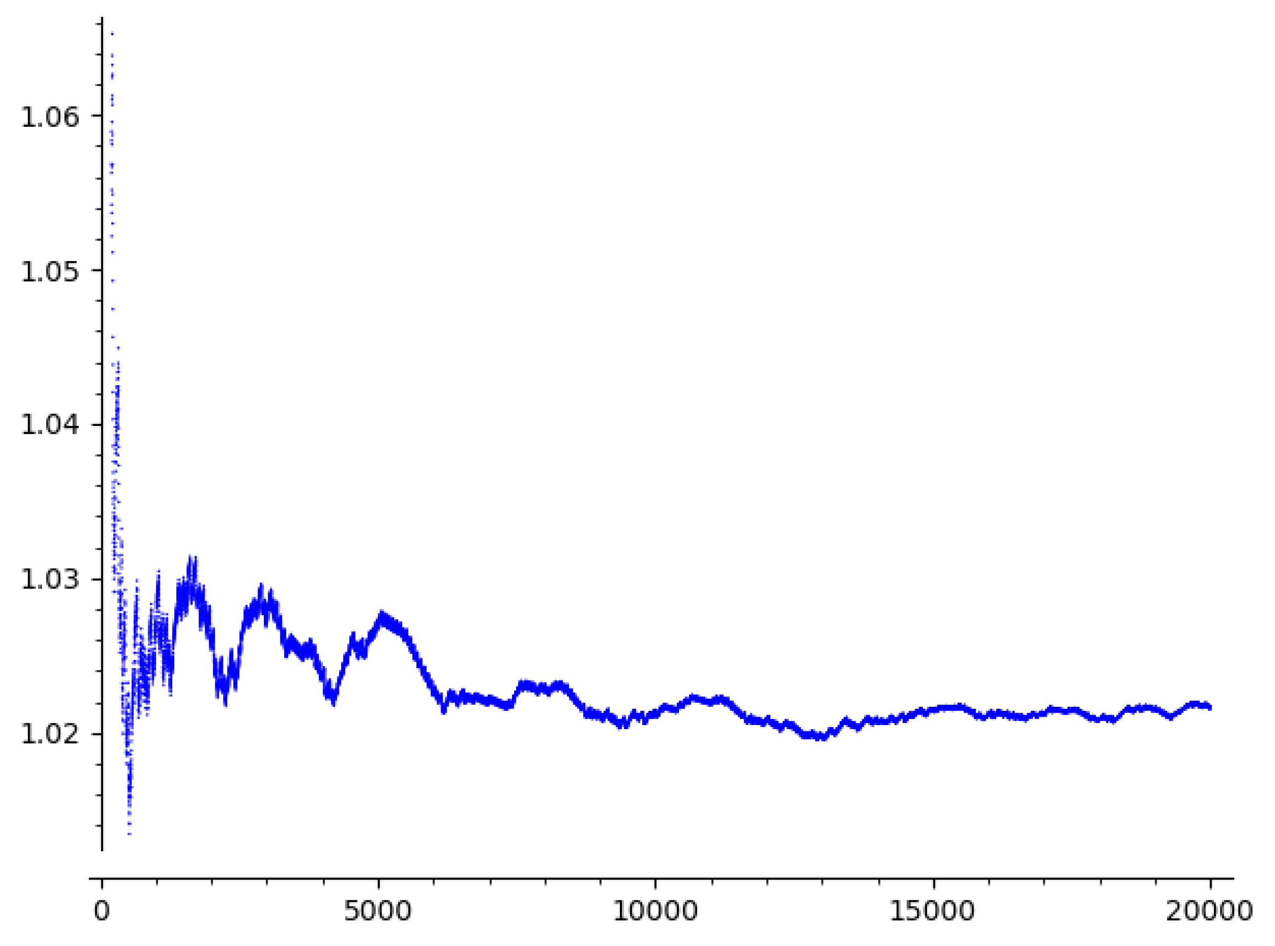
This sequence appears to diverge exponentially towards infinity and does not seem to reach a stable cycle. To illustrate this behavior, Figure 1 depicts

{(f^{\circ r} (73))}^{1 / r}

for iterations where

200 < r < 20000

From Figure 1, it is inferred that

f^{\circ r} (73) \sim δ^{r}

, with

δ \approx 1.02

Now, consider the probability, as in [9], of the first m terms of the sequence

f^{\circ r} (73)

being even, defined by:

p_{0} (m) : = \frac{| {r < m | f^{\circ r} (73) is even} |}{m} .

The probability that the first m terms are odd is then

p_{1} (m) : = 1 - p_{0} (m)

Computing the values of

p_{i} (m)

for

m = 10^{ℓ}

ℓ = 1, \dots, 5

, we observe an intriguing result:

It is surprising because

p_{0} (m)

does not converge to

1 / 2

, but instead to

α \approx 0.465

. This observation aligns with our earlier findings since:

δ \approx 1.02 \approx {\sqrt{2}}^{(0.535 - 0.465)} = {\sqrt{2}}^{(1 - 2 \times 0.465)} \approx {\sqrt{2}}^{(1 - 2 α)} .

\begin{matrix} ℓ & p_{0} (10^{ℓ}) & p_{1} (10^{ℓ}) \\ 1 & 0.2 & 0.8 \\ 2 & 0.45 & 0.55 \\ 3 & 0.467 & 0.533 \\ 4 & 0.4700 & 0.5300 \\ 5 & 0.46410 & 0.53590 \\ 6 & 0.465476 & 0.534524 \end{matrix}

For

ℓ = 6

, these results were obtained using Pari/GP with a precision of 15000 decimal digits. We computed

p_{1} (10^{6}) = 0.534524

, while the value of

f^{\circ 10^{6}} (73)

is approximately

3.89439 \times 10^{10394}

, necessitating such high precision. The logarithm

{log}_{73} ()

of this value is

5578.52

This raises several questions: Does

f^{\circ r} (73)

indeed avoid cycles? Does

{(f^{\circ r} (73))}^{1 / r}

converge to

δ \approx 1.02

? Does

p_{0} (m)

converge to

α \approx 0.465

, and is it true that

δ^{2 α} = 2

? What are the precise values of

δ

and

α

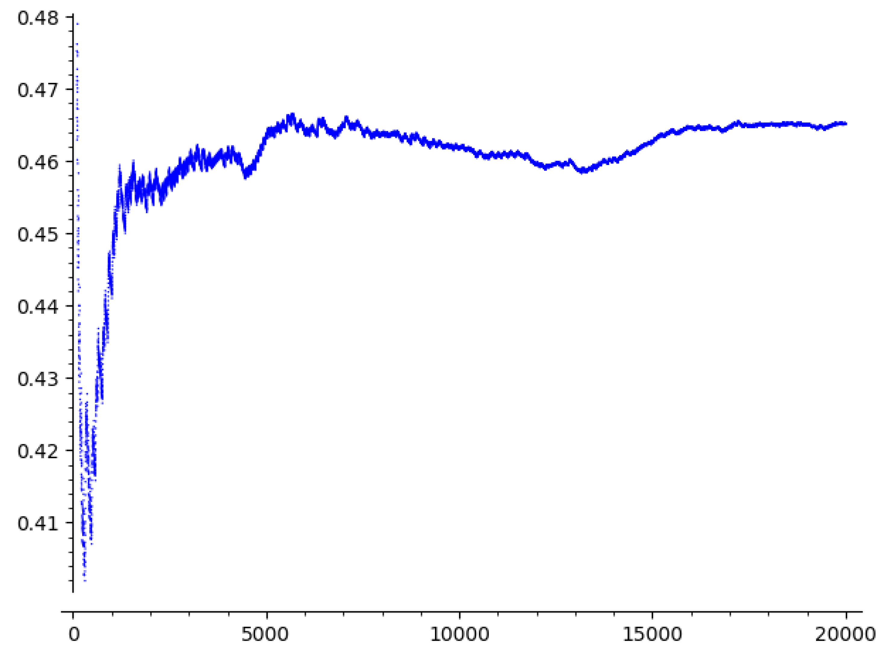
Figure 2 shows the values of

p_{0} (m)

for

100 < m < 20000

This behavior is not exclusive to

n = 73

but seems to manifest more frequently as n increases. For example, for

n < 100

, this phenomenon occurs only for

n = 73

, but for

n < 200

, it occurs for the values

n = 73, 103, 104, 105, 107, 141, 145, 146, 147, 148, 149, 151, 152, 153, 155, 161, 175, 199

. For

10000 \leq n < 11000

, exactly 954 numbers exhibit this behavior.

Below, in Figure 3, we present the corresponding plot for

n = 123456789

A natural question arises: does this phenomenon occur for almost all n? If so, does it occur with natural density 1, and does it involve the same constant

α

For numbers

n < 10000

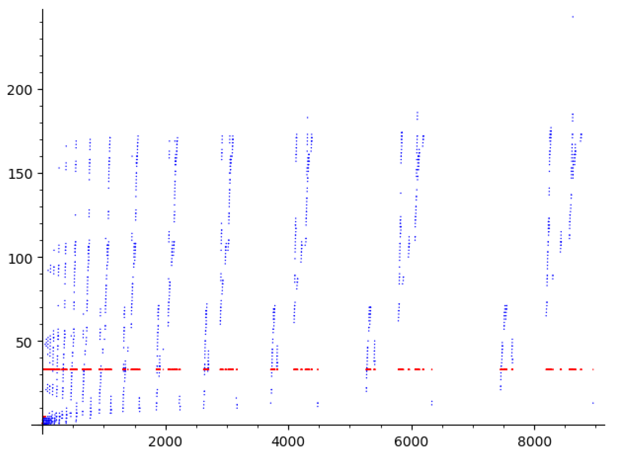
, there are exactly 1535 values of n for which this phenomenon does not occur. Figure 4 shows, for such n, the minimal m (in blue) such that

f^{\circ m} (n) = f^{\circ (m + r)} (n)

for some

r > 0

, along with the minimal r (in red):

In fact, all of these numbers eventually reach the same cycle of length 33:

(15, 21, 29, 41, 57, 80, 56, 39, 55, 77, 108, 76, 53, 74, 52, 36, 25, 35, 49, 69, 97, 137, 193, 272, 192, 135, 190, 134, 94, 66, 46, 32, 22)

with the exception of:

7, 8, 9, 10, 12, 13, 14, 18, 19, 20, 26, 27, 28, 38, 40, 54,

which fall into the cycle

(5, 7, 9, 12, 8)

, and the numbers

1, 2, 3, 4, 6

that reach

(1)

, with

f (0) = 0

If this pattern continues indefinitely, there must exist infinitely many such n. This prompts further inquiry: Are there infinitely many n that reach a cycle? Do all such n converge to the same cycle of length 33, apart from the exceptions listed above? Is there an explicit formula for these numbers n?

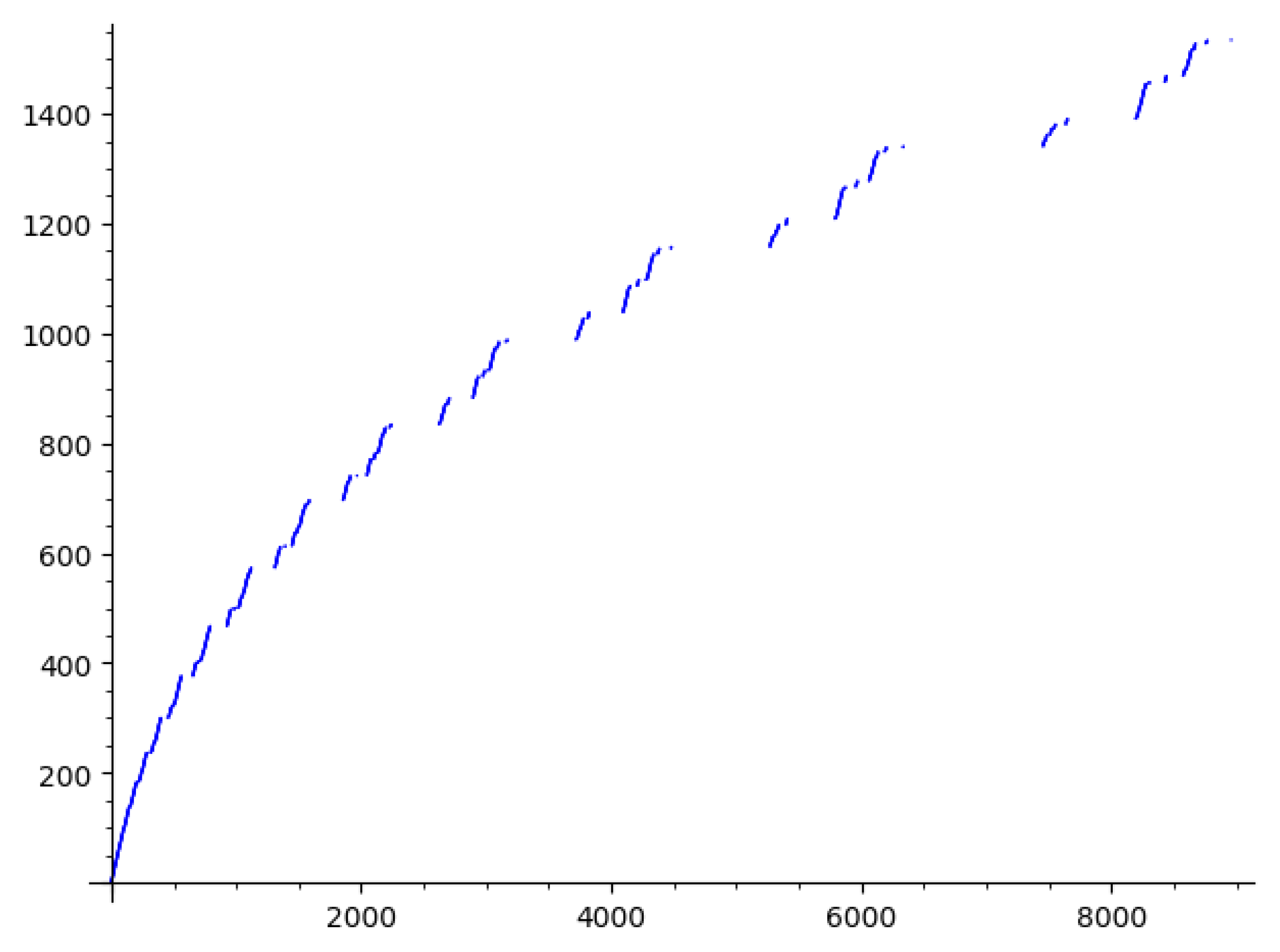
Figure 5 shows the counting function for these phenomena, which appears logarithmic:

4. Analysis of the First Result

We consider pairs of

(m, n)

as in [2], where m is consecutive to its 1-step predecessor n, such that

f (n) = m

. When

n = 0

, it indicates that m has no predecessor. I overlooked the possibility that one m can have two predecessors, but if

n / 2

is odd, then

n / 2

serves as a second predecessor [7]. This makes the table more intriguing, as all odd predecessors n are overwritten by even predecessors

2 n

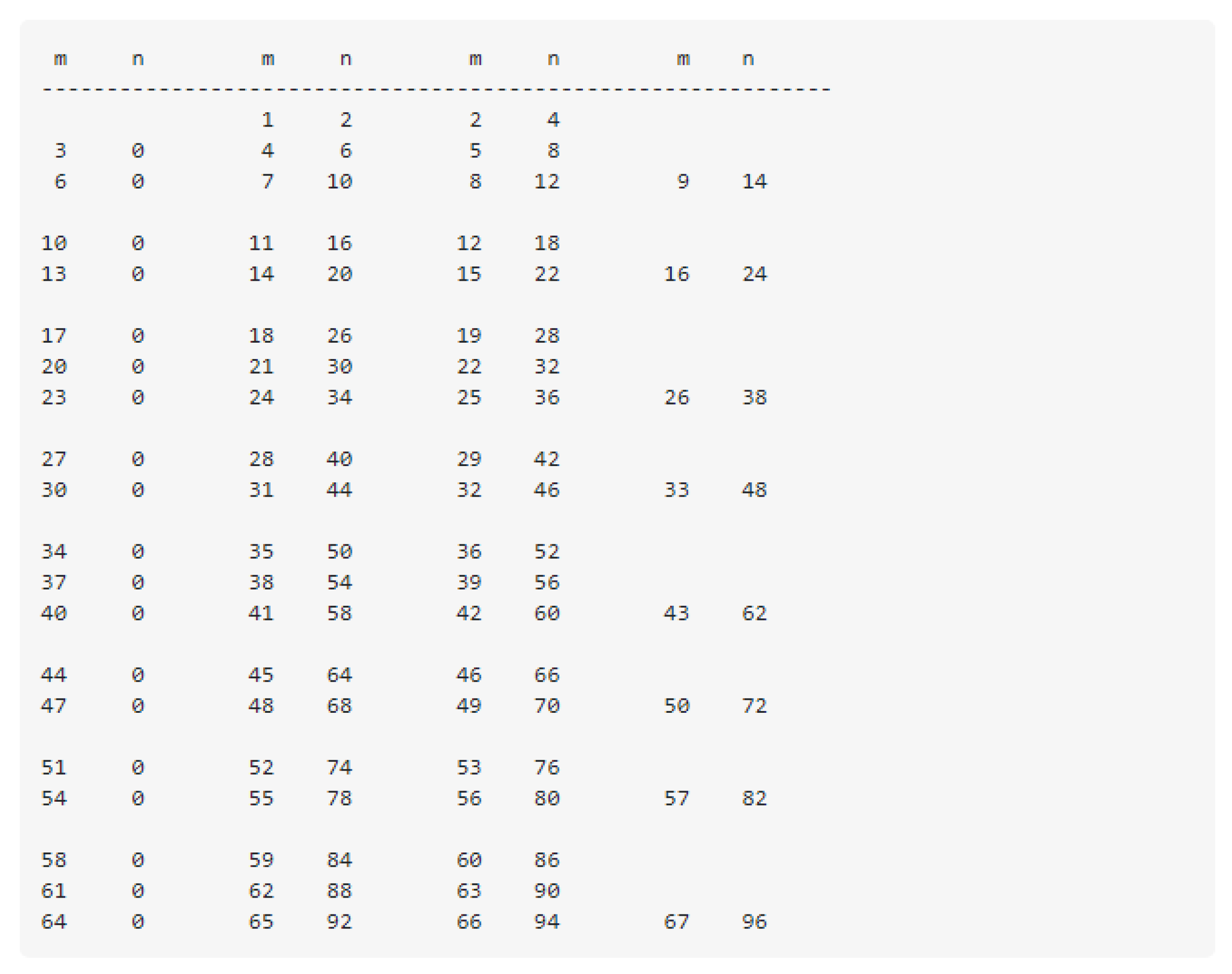
Moreover, an almost periodic structure emerges. We tried to capture this by arranging three or four columns of

(m, n)

such that the first column includes all m without a predecessor. Although the basic pattern is not truly periodic, there are super-patterns that appear periodic but ultimately are not. This pattern-superpattern structure is also recursive, reminiscent of a similar structure I found when examining

β = {log}_{2} (3)

, where a comparable pattern-superpattern-supersuperpattern emerged, linked to the continued fraction expansion of

β

. Therefore, we suspect there will be no simple description for the cases where m lacks a predecessor.

Figure 6. Interpretation table for predecessors of the observed phenomenon

Now, let’s further explain the concept of a "recursive aperiodic pattern." Listing the values of m with no predecessor, we get:

m_k: 3, 6, 10, 13, 17, 20, 23, 27, 30,...

By writing out the differences (with a zero prepended to the list of

m_{k}

0, 3, 3, 4, 3, 4, 3, 3, 4, 3, 4,...

We observe a pattern of two distinct sequences: `3, 3, 4` and `3, 4`, repeating in an aperiodic manner. Let’s denote the longer sequence as `A` and the shorter one as `a`, with `A` representing a difference of 10 and `a` representing a difference of 7. This gives us:

Aa Aa Aaa

Aa Aaa

Aa Aa Aaa

Aa Aaa

Aa Aa Aaa

Aa Aaa

Again, only two types of sequences emerge. Let’s further simplify: `Aaa` becomes `B`, and `Aa` becomes `b`. Now, `B` represents a difference of 24, and `b` represents a difference of 17. This leads to:

bbB bB

bbB bB bB

bbB bB

bbB bB bB

bbB bB

The next step yields:

Cc Cc Ccc

Cc Ccc

Cc Cc Ccc

Cc Ccc

Cc Cc Ccc

Cc Ccc

Here, `c` represents a difference of

17 + 24 = 41

, and `C` represents a difference of

17 + 17 + 24 = 58

. This continues recursively.

This recursive pattern seems to mirror a similar one related to

β = {log}_{2} (3)

, where the structure reflected the convergents of the continued fraction expansion of

β

. Interestingly, the early differences in this case match the convergents of the continued fraction expansion of

\sqrt{2}

a b c short patterns

--------------------------------------

[1 1 3 7 17 41 99 239 577 ... ] convergents of contfrac(sqrt(2))

[0 1 2 5 12 29 70 169 408 ... ]

--------------------------------------

A/2 B/2 C/2 long patterns

This can be explained by the following:

(1) A number of the form $⌊ 2 k \sqrt{2} ⌋$ has exactly one predecessor, $4 k$ .
(2) A number of the form $⌊ (2 k - 1) \sqrt{2} ⌋$ has two predecessors: $2 k - 1$ and $4 k - 2$ .
(3) A number has no predecessors if it is of the form $⌊ n (2 + \sqrt{2}) ⌋$ .

Using a recursive back-step algorithm, we constructed the predecessor tree for

m = 73

. If there are no errors, the tree should be complete, but the results should be checked for possible bugs.

The back-steps move diagonally from the top-right to the southwest. When there are two possible predecessors, they are placed in the same column but on different rows. If a predecessor has no further predecessor, a short line (`—`) is printed.

73 <--- start

104

148

105 ---

210

149

212

300 ---

298

211 ---

422

299

424

600 ---

598

423 ---

846 ---

----------------------------- tree seems complete (please verify!)

We can offer a heuristic proof for these results using the Beatty theorem [19], which states:

Theorem 1.

Given an irrational number

r > 1

, there exists

s > 1

such that the Beatty sequences

B_{r}

and

B_{s}

partition the set of positive integers, with each integer belonging to exactly one sequence.

Proof.

Applying the Beatty theorem (Theorem 1), let

A = {E (n (\sqrt{2} + 2)); n \in N^{*}}

and

B = {E (n \sqrt{2}); n \in N^{*}}

, which form a partition of

N^{*}

. We also have

E (n (\sqrt{2} + 2)) = 2 n + E (n \sqrt{2})

, where E denotes the floor function. This proves part of Result 2 regarding numbers without predecessors.

For the first result, assume that the probability of an integer n being odd is

\frac{1}{2}

and that the probability of

f (n)

being odd when n is even (or odd) is also

\frac{1}{2}

. We observe that this probability does not remain

\frac{1}{2}

for

f^{\circ r} (n)

when

r \geq 2

. In some sense, the probability does not commute with the composition of f with itself.

(1) If n and $m = f (n)$ are even: Since $\frac{n}{\sqrt{2}} = m + θ$ (with $0 < θ < 1$ ), we have $m = \frac{n}{\sqrt{2}} - θ$ . Then,

$f^{\circ 2} (n) = f (m) = ⌊\frac{m}{\sqrt{2}}⌋ = ⌊\frac{\frac{n}{\sqrt{2}} - θ}{\sqrt{2}}⌋ = ⌊\frac{n}{2} - \frac{θ}{\sqrt{2}}⌋ .$

However, $\frac{n}{2}$ is even with probability $\frac{1}{2}$ , so in this case, $f^{\circ 2} (n)$ is odd with probability $\frac{1}{2}$ .

□

5. Homoclinic Orbits and Chaos in the Unperturbed System Using the Collatz Problem

While a universally accepted definition of chaos is elusive, a widely utilized definition, originally proposed by Robert L. Devaney, stipulates that for a dynamical system to be classified as chaotic, it must exhibit the following properties:

1) Sensitivity to initial conditions
2) Topological mixing
3) Dense periodic orbits

We begin by considering the harmonically driven damped pendulum, a quintessential example of a chaotic system, described by the equation

\ddot{ϕ} + \frac{1}{q} \dot{ϕ} + sin ϕ = A cos (ω t)

(1)

For small values of A and

ω

, the system behaves like a driven harmonic oscillator, asymptotically settling into regular oscillations with a fixed period. However, as A or

ω

increases while keeping other parameters fixed, the system undergoes a cascade of period-doubling bifurcations that lead to chaotic behavior, followed by a return to regular oscillations when the parameters are increased further. For instance, with

q = 2

and

ω = 2 / 3

, the first period doubling (termed "symmetry breaking") occurs at

A \approx 1.07

, with the onset of chaos at

A \approx 1.08

. These rigorous results are derived from numerical simulations. Notably, one may inquire about conditions on A,

ω

, and q that keep the system below the first period doubling; however, this question lies beyond the scope of our study. It remains intriguing to explore chaotic behaviors in some dynamics and discover new methods to suppress chaos in the cubic-quintic Duffing equation using discrete iterated maps, which is the central focus of our research.

For the unperturbed system with fractional-order displacement, when

ε = 0

, the differential equation (1) can be reformulated as follows for

A = 0

\ddot{x} - a x + b x^{3} + c x^{5} = 0

(2)

Let us define

Δ : = b^{2} + 4 a c

(3)

The equilibrium points for

Δ > 0

are given by:

(x, \dot{x}) = (\pm \sqrt{\frac{- b + \sqrt{b^{2} + 4 a c}}{2 c}}, 0) : centers

(4)

We define:

x_{e}^{+} = \sqrt{\frac{- b + \sqrt{b^{2} + 4 a c}}{2 c}} and x_{e}^{-} = - \sqrt{\frac{- b + \sqrt{b^{2} + 4 a c}}{2 c}}

(5)

The energy function for (2) is expressed as:

\frac{1}{2} \dot{x} {(t)}^{2} - \frac{1}{2} a x {(t)}^{2} + \frac{1}{4} b x {(t)}^{4} + \frac{1}{6} c x {(t)}^{6} = K

(6)

where K is the energy constant that depends on the initial amplitude

x (0) = x_{0}

and the initial velocity

x^{'} (0) = {\dot{x}}_{0}

K = \frac{1}{2} {\dot{x}}_{0}^{2} - \frac{1}{2} a x_{0}^{2} + \frac{1}{4} b x_{0}^{4} + \frac{1}{6} c x_{0}^{6}

(7)

Depending on K, the level sets vary. For all cases, these level sets form closed periodic orbits surrounding the fixed points

(x, \dot{x}) = (x_{e}^{+}, 0)

(x, \dot{x}) = (x_{e}^{-}, 0)

or all three fixed points

(x_{e}^{\pm}, 0)

and

(0, 0)

. The boundary separating these two groups of orbits corresponds to

K = 0

, when

{\dot{x}}_{0} = \pm x_{0} \sqrt{\frac{1}{6} (6 a - 3 b x_{0}^{2} - 2 c x_{0}^{4})}

(8)

The level set

\frac{{\dot{x}}^{2}}{2} - \frac{1}{2} a x^{2} + \frac{1}{4} b x^{4} + \frac{1}{6} c x^{6} = 0

(9)

consists of two homoclinic orbits:

Γ_{+}^{0} (t) \equiv (x_{+}^{0} (t), {\dot{x}}_{+}^{0} (t))

(10)

Γ_{-}^{0} (t) \equiv (x_{-}^{0} (t), {\dot{x}}_{-}^{0} (t))

(11)

which connect the fixed hyperbolic saddle point

(0, 0)

to itself, containing the stable and unstable manifolds. The functions

x_{\pm}^{0} (t)

can be evaluated using the following formulas:

M (t_{0}) = \int_{- \infty}^{+ \infty} {\dot{x}}^{0} (t) [γ cos ω (t + t_{0}) - δ {\dot{x}}^{0} (t)] d t

(12)

with

x^{0} (t) = \frac{A \sec h (\sqrt{k} t)}{\sqrt{1 + λ \cdot {\sec h}^{2} (\sqrt{k} t)}}

(13)

See Figure 5.

The homoclinic orbit [21] delineates the phase plane into two regions. Within the separatrix curve, the orbits are confined around one of the centers, while outside the separatrix curve, the orbits encircle both centers and the saddle point. Physically, this implies that for certain initial conditions, the oscillations are centered around one steady-state position [23], while for others, they encompass all steady-state solutions (two stable and one unstable).

In the second scenario, where we utilize the iterated map (Collatz-like problem sequences) as the right-hand side of equation (1), we note a transition to chaos, indicated by sensitivity to initial conditions. Consider the following initial value problem (IVP):

\ddot{x} - a x + b x^{3} + c x^{5} = f, \dot{x} (0) = 0, x (0) = 0

(14)

where

f : n \mapsto \{\begin{matrix} ⌊n / \sqrt{2}⌋ & if n even, \\ ⌊n \sqrt{2}⌋ & if n odd . \end{matrix}

Let

f^{\circ (r + 1)} : = f \circ f^{\circ r}

and consider the orbit of

n = 73

for iterations of f, i.e., the sequence

f^{\circ r} (73)

73, 103, 145, 205, 289, 408, 288, 203, 287, 405, 572, 404, 285, 403, 569, 804, 568, 401, \dots

This sequence appears to diverge to infinity exponentially and, notably, never reaches a cycle. This is illustrated in the following figure of

{(f^{\circ r} (73))}^{1 / r}

for

200 < r < 20000

(see Figure 7).

In conclusion, while traditional chaotic behavior manifests through properties like sensitivity to initial conditions and topological mixing, the exploration of orbits and sequences like those derived from the Collatz problem offers a fascinating perspective on understanding chaos in dynamical systems.

6. Density of the Given Sequence Using Riemannian Metric

In this section, we may proceed with discussing the density value of our sequence, defined as

f (n) = \{\begin{matrix} ⌊\frac{n}{\sqrt{2}}⌋ & if n is even, \\ ⌊n \sqrt{2}⌋ & if n is odd . \end{matrix}

in Riemannian and Euclidean metrics. We will compare the obtained density values and try to find the lower and upper bounds of these densities in both spaces using theoretical and numerical approaches. Understanding the density of a sequence in a Riemannian metric space is crucial for analyzing its distribution and behavior. The choice of a Riemannian metric allows us to account for the geometric properties of the manifold, which can significantly impact how points are distributed. This approach is essential when examining sequences that may exhibit non-standard distributions or clustering behavior.

The Riemannian metric used to calculate the density in this space is defined as:

g (x, y) = exp (- α \cdot | f (x) - f (y) |)

where

f (x)

is the value of the sequence at index x, and

α

is a constant that controls the influence of the metric on distances between points. The metric diminishes exponentially as the absolute difference between

f (x)

and

f (y)

increases, emphasizing points that are close in value under the sequence.

To define the density function in a Riemannian metric space, consider the following formulation. Given a Riemannian manifold

(M, g)

where g is the Riemannian metric, the density function

ρ : M \to R

for a sequence

(f (n))

can be defined as:

ρ (x) = lim_{ϵ \to 0} \frac{1}{V (B_{ϵ} (x))} \int_{B_{ϵ} (x)} χ (f (n)) d V

where

B_{ϵ} (x)

is a geodesic ball of radius

ϵ

centered at x,

V (B_{ϵ} (x))

is the volume of this ball, and

χ (f (n))

is the characteristic function indicating the presence of points from the sequence within the ball.

The importance of using a Riemannian metric lies in its ability to provide insights into the behavior of the sequence in relation to the manifold’s curvature and topology. By analyzing the density function, we can uncover information about how the sequence is concentrated in various regions of the metric space, potentially revealing patterns that would remain hidden in a standard Euclidean setting.

In the subsequent analysis, we will explore the density of the given sequence using the Riemannian metric, focusing on its distribution and characteristics.

6.1. Analysis of the Density Plot

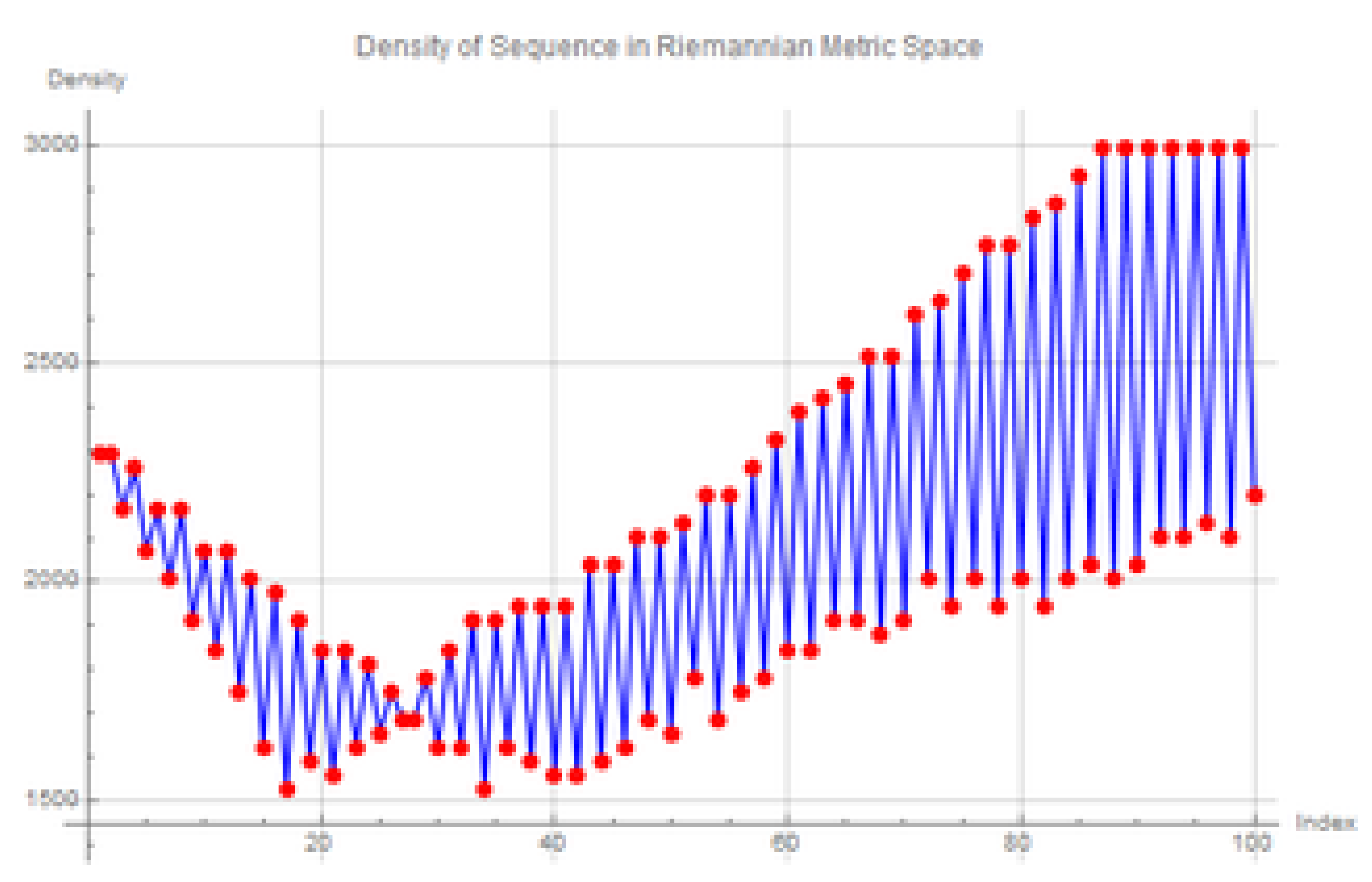
The provided density plot illustrates the distribution of a sequence in a Riemannian metric space. The x-axis represents the index of the sequence, while the y-axis indicates the density calculated using the Riemannian metric with a value of

α = 0.1

. Analyzing the density of the sequence using Riemannian metrics is crucial for understanding how the sequence is distributed across the manifold, as it allows us to account for the geometric properties of the space in which the sequence resides.

Observations:

High density values: The plot exhibits consistently high density values throughout the sequence, suggesting a dense clustering of points in the metric space.
Oscillations: The density values show a slight oscillatory pattern, likely due to the nature of the sequence and the Riemannian metric.

Sensitivity to $α$ :

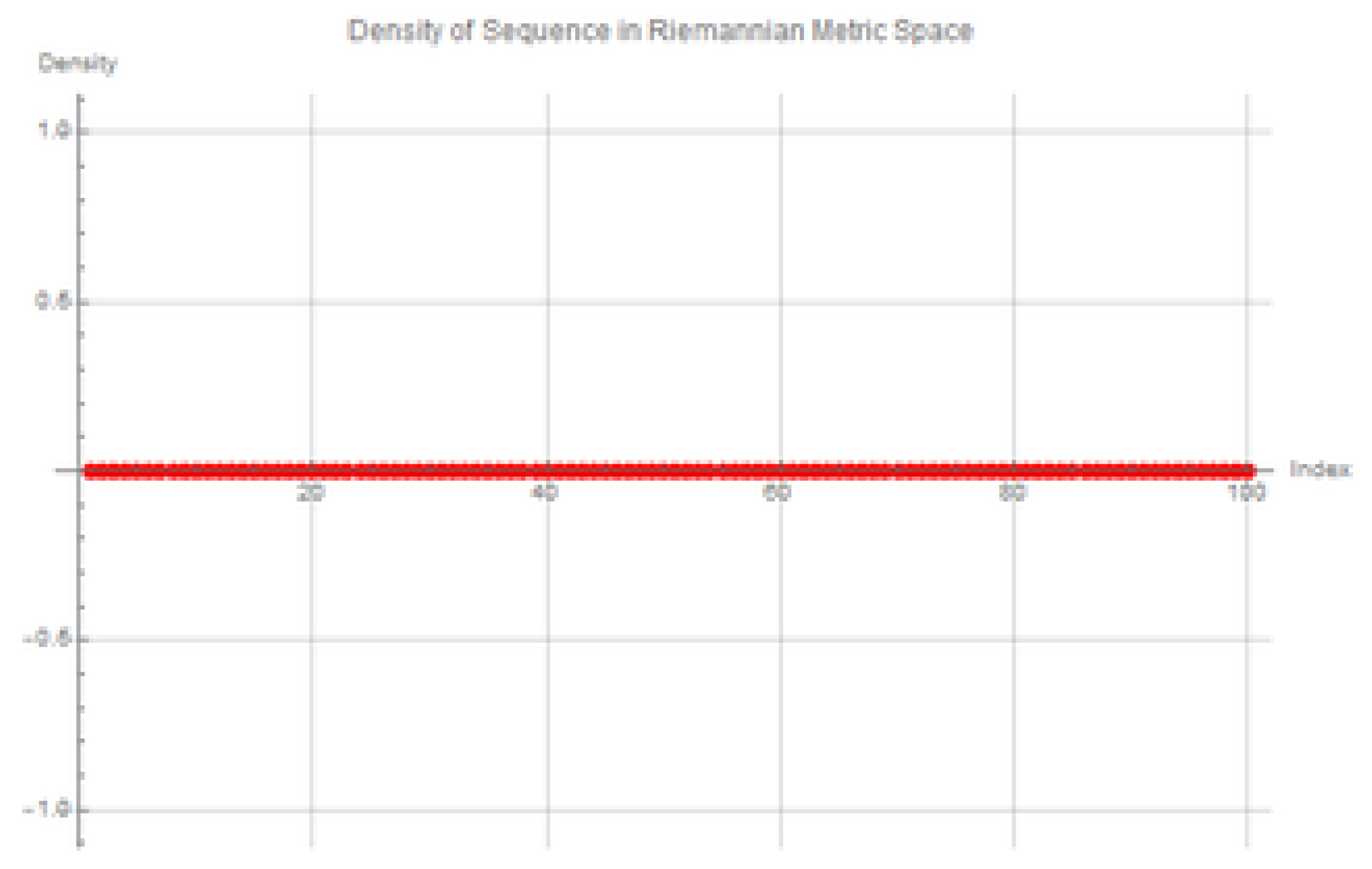
The density value is highly sensitive to the choice of

α

. Increasing the value of

α

results in more perturbations and higher density values, reflecting a denser clustering of sequence points. Conversely, as

α

approaches zero, the density tends to zero, aligning with the index of the sequence itself, represented as the red real line in the second figure. This indicates that the density diminishes significantly when the influence of the metric is reduced, highlighting the interplay between

α

and the sequence’s distribution.

Interpretation:

The high density values indicate that the sequence is concentrated in a specific region of the Riemannian metric space. This could be attributed to the inherent properties of the sequence, the choice of the Riemannian metric, or the value of

α

. The Riemannian metric captures the curvature and topology of the space, which influences how distances and densities are perceived, thus affecting the distribution of the sequence.

Further Analysis:

To gain a deeper understanding of the sequence’s behavior, consider:

Varying $α$ : Experiment with different values of $α$ to observe how the density profile changes. This will provide insight into the sensitivity of the density calculation to the choice of metric parameters.
Visualizing the sequence: Plot the sequence itself in the Riemannian metric space to visualize its distribution. Such visualizations can help identify clustering patterns and the overall structure of the sequence.
Calculating other metrics: Compute additional metrics, such as variance or entropy, to characterize the sequence’s distribution. These metrics can provide further context and quantify the spread and concentration of the sequence points.

Figure 8. Density plot of the sequence in Riemannian metric space

Figure 9. Sensitivity of density values to changes in

α

. The red line represents the index of the sequence as

α \to 0

Figure 9. Sensitivity of density values to changes in

α

. The red line represents the index of the sequence as

α \to 0

7. Analytical Estimation of the Sequence Density in Riemannian Geometry

In this section, we aim to analytically estimate the density of the given sequence using theories from Riemannian geometry. The sequence is defined as:

f (n) = \{\begin{matrix} ⌊\frac{n}{\sqrt{2}}⌋ & if n is even, \\ ⌊n \sqrt{2}⌋ & if n is odd . \end{matrix}

The Riemannian metric that we use to analyze this sequence is given by:

g (x, y) = exp (- α \cdot | f (x) - f (y) |)

This metric defines the geodesic distance between two points

f (x)

and

f (y)

, where

α > 0

is a parameter controlling the curvature and clustering behavior of the sequence. In this section, we will focus on estimating the density of the sequence in the context of Riemannian geometry.

7.1. Volume Growth in Riemannian Manifolds

One important property in Riemannian geometry is the growth of volume for geodesic balls in a manifold. The volume of a geodesic ball of radius r centered at a point p on an n-dimensional Riemannian manifold

(M, g)

grows asymptotically as:

V (B_{r} (p)) \sim C_{n} \cdot r^{n} \cdot exp (\sqrt{| K |} \cdot r)

where

C_{n}

is a constant depending on the dimension n, and K represents the sectional curvature. For small values of r, the volume growth is approximately polynomial, but for larger values, the curvature term introduces exponential growth. This relationship plays a crucial role in estimating the density of the sequence in our Riemannian metric space.

7.2. Density Function in Riemannian Metric

Given the Riemannian metric

g (x, y)

, the density of the sequence can be computed using the relationship between the volume of geodesic balls and the distance between points in the sequence. The density at a point

f (n)

can be expressed as the inverse of the volume of a small geodesic ball centered at

f (n)

. For small r, the volume of a geodesic ball

B_{r} (f (n))

is approximately:

V (B_{r} (f (n))) \sim r^{n} \cdot exp (- α \cdot | f (n) - f (n + r) |)

Thus, the density function

ρ (f (n))

is given by:

ρ (f (n)) = \frac{1}{V (B_{r} (f (n)))} \sim \frac{1}{r^{n}} \cdot exp (α \cdot | f (n) - f (n + r) |)

This shows that the density increases exponentially with

α

and the distance between points in the sequence.

7.3. Estimation of Growth Rate

We now estimate the growth rate of the density function for the given sequence. The sequence

f (n)

grows linearly in n, as:

f (n) \sim ⌊n \cdot \sqrt{2}⌋

This linear growth suggests that the distance between consecutive points

f (n)

and

f (n + 1)

O (1)

. Therefore, the geodesic distance between two points in the Riemannian space is

O (1)

for small n. For large n, the density function grows as:

ρ (f (n)) \sim exp (α \cdot n)

indicating that the density increases exponentially as n increases, driven by the Riemannian metric.

7.4. Bounds on the Density

Using the Riemannian metric

g (x, y)

, we can estimate upper and lower bounds for the density of the sequence. For large

α

, the density

ρ (f (n))

is dominated by the exponential term, and we can write:

ρ (f (n)) = O (exp (α \cdot n))

For small

α

, the density grows at a slower rate, and we can approximate:

ρ (f (n)) = O (n^{k}) for some constant k

This shows that the density of the sequence is highly sensitive to the value of

α

. As

α \to 0

, the density approaches zero, while for larger values of

α

, the density becomes increasingly concentrated.

The analytical estimation of the sequence’s density in a Riemannian manifold reveals an exponential dependence on the value of

α

, with the density growing rapidly as n increases. The Riemannian metric introduces a curvature-dependent growth that significantly affects how the points of the sequence are distributed. The use of Riemannian geometry allows for a deeper understanding of the clustering behavior and provides a theoretical framework for estimating both the upper and lower bounds of the density function. This analysis highlights the sensitivity of the density to the choice of the metric and the curvature of the space.

8. Analysis of the Density Plot in Euclidean Metric Space

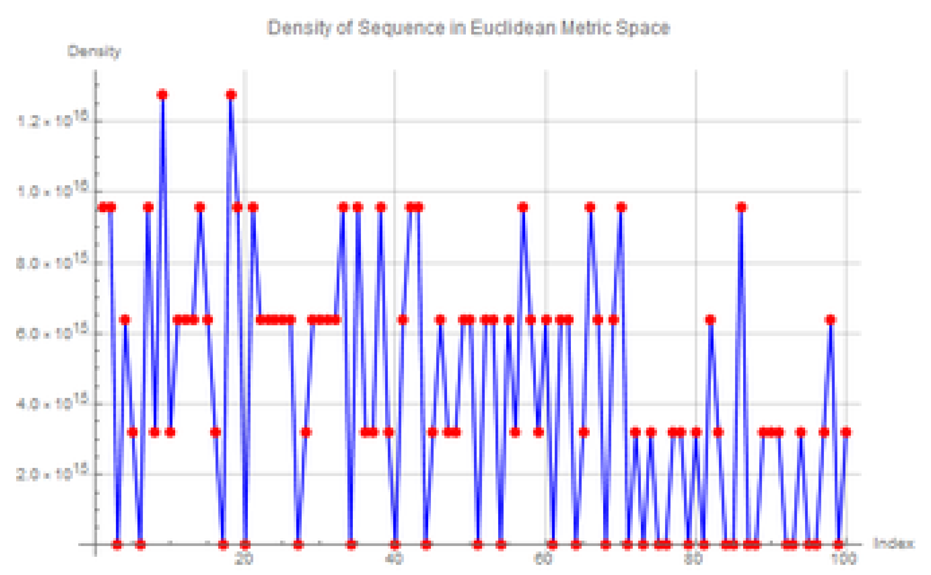
In this section, we proceed with analyzing the density of the given sequence in Euclidean metric space. The x-axis represents the index of the sequence, while the y-axis shows the density values calculated using the Euclidean metric. To compute the density in Euclidean space, we use the following formula for the Euclidean metric between two points x and y:

euclideanMetric [x, y] : = | f (x) - f (y) |

where

f (n)

is the sequence defined as:

f [n] : = \{\begin{matrix} ⌊\frac{n}{\sqrt{2}}⌋, & if n is even, \\ ⌊n \sqrt{2}⌋, & if n is odd . \end{matrix}

We analyze the density based on this metric for two different values of

ϵ

, starting with

ϵ = 0.0001

, followed by a case where

ϵ = 0.0000000001

to study the impact of smaller

ϵ

values.

8.1. Observations for $ϵ = 0.0001$

The density plot for

ϵ = 0.0001

is shown in Figure 10 below. The key features observed are:

Spikes and valleys: The plot shows distinct spikes and valleys, indicating significant fluctuations in density across the sequence.
Higher overall density: Compared to the Riemannian metric (see previous section), the density values in the Euclidean metric are generally higher. This suggests a denser distribution of points in the sequence under the Euclidean metric.
Localized peaks: Several localized peaks can be observed, indicating specific regions where the sequence is particularly concentrated.

8.2. Effect of $ϵ = 0.0000000001$

Next, we consider the density plot for an extremely small value of

ϵ = 0.0000000001

, shown in Figure 11 below. The key observations in this case are:

Sharp increase in density: When $ϵ$ is reduced to 0.0000000001, the density values increase sharply compared to the case with $ϵ = 0.0001$ . This demonstrates the high sensitivity of the density to $ϵ$ in Euclidean space.
Higher fluctuations: The density plot exhibits more intense fluctuations, with sharper spikes and deeper valleys. This suggests that the density becomes more localized around the sequence points as $ϵ$ decreases.
Persistence of peaks: Despite the increase in density values, the peaks and valleys remain at similar positions in the plot, suggesting that the fundamental distribution pattern of the sequence is unchanged. The smaller $ϵ$ simply amplifies the magnitude of the density at those positions.

8.3. Interpretation and Sensitivity to $ϵ$

The observed pattern in Euclidean metric space indicates that the sequence exhibits more clustered behavior and is less uniformly distributed compared to the Riemannian metric. The sharp increase in density values when

ϵ

is small (

ϵ = 0.0000000001

) shows that the density is highly sensitive to the choice of

ϵ

Density magnitude: In the Euclidean metric, density values are generally higher than in the Riemannian metric (as seen in previous sections). This reflects a denser clustering of sequence points.
Effect of $ϵ$ : As $ϵ$ decreases, the density increases rapidly, leading to a denser and more localized distribution around specific points in the sequence. This behavior is especially evident in Figure 11, where smaller $ϵ$ values lead to an "explosion" of density at certain indices.
Comparison with Riemannian Metric: Compared to the Riemannian metric, where the density was more spread out and smoother, the Euclidean metric reveals a more clustered, localized distribution. This suggests that the flatness of Euclidean space causes points to be more tightly packed when measured using this metric.

The key takeaway from this analysis is that the density of the sequence in Euclidean space is highly sensitive to the choice of

ϵ

. For very small values of

ϵ

, we observe sharp increases in density, indicating that points in the sequence become more densely packed around specific regions, as visualized in Figure 10 and Figure 11.

9. Analytical Estimation of Density Growth Rate in Euclidean Metric Space

In this section, we aim to estimate the growth rate of the density of the given sequence analytically in the context of Euclidean metric space. We will employ big O notation and advanced theories from sequence density estimation, leveraging the cardinality of the sequence.

9.1. Density Function Definition

The density of a sequence in Euclidean metric space at a given point can be defined as the number of points in the sequence within a certain radius

ϵ

divided by the area of the surrounding space. For a sequence S of cardinality

# (S)

, the density function D can be expressed as:

D (n, ϵ) = \frac{1}{Volume (B (n, ϵ))} \cdot # (S \cap B (n, ϵ))

where

B (n, ϵ)

represents a ball of radius

ϵ

centered at point n.

9.2. Growth Rate Estimation in Euclidean Space

To estimate the growth rate of density as n increases in the Euclidean metric space, we analyze the asymptotic behavior of the density function:

D (n, ϵ) = \frac{# (S \cap B (n, ϵ))}{C ϵ^{d}}

where C is a constant and d is the dimensionality of the space (here,

d = 1

for our discrete sequence).

We investigate how the cardinality

# (S \cap B (n, ϵ))

behaves as n increases. Given that our sequence

f (n)

oscillates based on whether n is even or odd, we can deduce that the number of elements within any

ϵ

-neighborhood grows as follows:

1. For small values of

ϵ

, the cardinality grows logarithmically:

# (S \cap B (n, ϵ)) = O (\frac{1}{ϵ})

2. Thus, the density in Euclidean metric can be approximated as:

D (n, ϵ) = O (\frac{1 / ϵ}{C ϵ}) = O (\frac{1}{C ϵ^{2}})

This indicates that as we decrease

ϵ

, the density

D (n, ϵ)

can potentially grow without bound, particularly in regions of high clustering within the sequence.

The analysis shows that the growth rate of density of the given sequence in Euclidean metric space is highly sensitive to the choice of

ϵ

. Specifically, using big O notation, we find that:

D (n, ϵ) = O (\frac{1}{ϵ^{2}})

This implies that even small changes in

ϵ

can lead to significant variations in density, especially in regions where the sequence exhibits clustering behavior. As such, careful selection of

ϵ

is crucial for accurately estimating the density of the sequence in Euclidean metric space.

Data Availability Statement

This work is based on the research of Sebastien Palcoux in his ArXiv paper titled "Unexpected Behavior of Some Transcendental Number Like

\sqrt{2}

" [22]. All the data and theoretical results used in this study are derived from the mentioned paper, and no additional datasets were generated during the current study. Further details on the foundational concepts and sequence behavior can be referenced from Palcoux’s work.

Acknowledgments

The authors would like to express their deep gratitude to Sebastien Palcoux for his pioneering work and insightful contribution in his paper "Unexpected Behavior of Some Transcendental Number Like

\sqrt{2}

" [22]. His innovative approach to analyzing sequences has been instrumental in shaping the direction of this study, providing key ideas that have allowed us to extend the theoretical understanding of sequence density in both Euclidean and Riemannian metrics.

Conflicts of Interest

The authors declare that they have no known competing financial interests or personal relationships that could have appeared to influence the work reported in this paper.

Appendix

Computation:

sage: for i in range(3,26):

....: print(sq2(i))

....:

[1/4*sqrt(2) + 1/8, 0.478553390593274]

[1/16*sqrt(2) + 7/16, 0.525888347648318]

[3/32*sqrt(2) + 13/32, 0.538832521472478]

[15/64*sqrt(2) + 13/64, 0.534581303681194]

[5/128*sqrt(2) + 61/128, 0.531805217280199]

[39/256*sqrt(2) + 81/256, 0.531852847392776]

[93/512*sqrt(2) + 141/512, 0.532269260352925]

[51/1024*sqrt(2) + 473/1024, 0.532348527032254]

[377/2048*sqrt(2) + 557/2048, 0.532303961432938]

[551/4096*sqrt(2) + 1401/4096, 0.532283123258685]

[653/8192*sqrt(2) + 3437/8192, 0.532285334012406]

[3083/16384*sqrt(2) + 4361/16384, 0.532288843554459]

[3409/32768*sqrt(2) + 12621/32768, 0.532289246647030]

[7407/65536*sqrt(2) + 24409/65536, 0.532288816169701]

[22805/131072*sqrt(2) + 37517/131072, 0.532288667983386]

[24307/262144*sqrt(2) + 105161/262144, 0.532288700334941]

[72761/524288*sqrt(2) + 176173/524288, 0.532288728736551]

[159959/1048576*sqrt(2) + 331929/1048576, 0.532288729880941]

[202621/2097152*sqrt(2) + 829741/2097152, 0.532288725958633]

[639131/4194304*sqrt(2) + 1328713/4194304, 0.532288724978704]

[1114081/8388608*sqrt(2) + 2889613/8388608, 0.532288725350163]

[1825983/16777216*sqrt(2) + 6347993/16777216, 0.532288725570602]

[5183461/33554432*sqrt(2) + 10530125/33554432, 0.532288725561857]

Code:

def sq2(n):

c=0

for i in range(2^n):

l=list(Integer(i).digits(base=2,padto=n))

if l[-1]==1:

cc=1/4

for j in range(n-2):

ll=[l[j],l[j+1],l[j+2]]

if ll==[0,0,0]:

cc*=1/2

if ll==[0,0,1]:

cc*=1/2

if ll==[0,1,0]:

cc*=(1-sqrt(2)/2)

if ll==[0,1,1]:

cc*=sqrt(2)/2

if ll==[1,0,0]:

cc*=1

if ll==[1,0,1]:

cc=0

break

if ll==[1,1,0]:

cc*=(1-sqrt(2)/2)

if ll==[1,1,1]:

cc*=sqrt(2)/2

c+=cc

return [c.expand(),c.n()]

M (t_{0}) = \int_{- \infty}^{+ \infty} {\dot{x}}^{0} (t) [γ cos ω (t + t_{0}) - δ {\dot{x}}^{0} (t)] d t,

(15)

Let

x^{0} (t) = \frac{A \sec h (\sqrt{k} t)}{\sqrt{1 + λ \cdot {\sec h}^{2} (\sqrt{k} t)}} .

(16)

References

J.J. O Connor and E.F. Robertson, Lothar Collatz, St Andrews University School of Mathematics and Statistics, Scotland; (2006).
H. Niederreiter and I. E. Shparlinski. Dynamical systems generated by rational functions. In Applied Algebra, Algebraic Algorithms and Error-Correcting Codes (Toulouse, 2003), volume 2643 of Lecture Notes in Comput. Sci., pages 6â€“17. Springer, Berlin, 2003.
Livio Colussi, The convergence classes of Collatz function, Theoretical Computer Science; vol.412 issue 39 pp. 5409â€“5419 (2011).
Jeffrey C. Lagarias and Daniel J. Bernstein. The 3x+1 conjugacy map. Canadian journal of mathematics 1996, 48, 1154–116. [Google Scholar] [CrossRef]
Alex V. Kontorovich, Yakov G.Sinai, Structure theorem for (d,g,h)-Maps, https://arXiv.org/abs/math/0601622,2006.
G. H. Hardy and E. M. Wright, An Introduction to the Theory of Numbers, Oxford university; (2008).
Poonen, B.: Characterizing integers among rational numbers with a universal-existential formula. Am. J. Math. 131(3), 675â€“682 (2009).
van der Poorten, A.J. Solution de la conjecture de pisot sur le quotient de Hadamard de deux fractions rationnelles. CR Acad. Sci. Paris 1988, 306, 102. [Google Scholar]
Rabin, M.O. Probabilistic algorithm for testing primality. J. Number Theory 1980, 12, 128–138. [Google Scholar] [CrossRef]
Shalev, A.: Some results and problems in the theory of word maps. In: Erdos Centennial, pp. Springer (2013).
Smith, A.: The congruent numbers have positive natural density. Preprint (2016). arXiv:1603.08479.
Tao, Z. On the representation of large odd integer as a sum of three almost equal primes. Acta Mathematica Sinica 1991, 7, 259–272. [Google Scholar] [CrossRef]
Collatz, L. On the origin of the (3n+1) problem. Journal of Qufu Normal University, Natural Science Edition 1986, 12, 9–11. [Google Scholar]
Lagarias, J.C.: The 3x+1 problem: An annotated bibliography (1963â€“2000). ArXiv math (NT0608208) (2006).
Wirsching, G.J.: The Dynamical System Generated by the 3n+1 Function. Lecture Notes in Mathematics, vol. 1681. Springer, Berlin (1981).
Hata, M. Rational Approximations to pi and Some Other Numbers. Acta Arith. 1993, 63, 335–349. [Google Scholar] [CrossRef]
Amdeberhan, T. and Zeilberger, D. q-ApÃ©ry Irrationality Proofs by q-WZ Pairs. Adv. Appl. Math. 1998, 20, 275–283. [Google Scholar] [CrossRef]
Oliveira e Silva, T. "Computational Verification of the 3x+1 Conjecture." Sep. 19, 2008. http://www.ieeta.pt/~tos/3x+1.
John William Strutt, 3rd Baron Rayleigh (1894). The Theory of Sound. Vol. 1 (Second ed.). Macmillan. p. 123.
H.W. Haslach H.W. Haslach . “Post-buckling behavior of columns with non-linear constitutive equations,” In ternational Journal of Non-Linear Mechanics 20.
P. Holmes& J. Marsden P. Holmes& J. Marsden.`A partial differential equation with infinitely many periodic orbits: chaotic oscillations of a forced beam,”Archives for Rational,Holmes, Philip and Marsden, Jerrold E.,292,419-448.
Sebastien Palcoux.Unexpected behavior involving 2 and parity,2020 https://mathoverflow.net/q/353493/51189.
Pyragas,1996 Pyragas,, "Continuous control of chaos by self controlling feedback", Academic Press, San Diego,, pp. 118-123.
Zeraoulia, R.: Amazing behavior and transition to chaos of some sequences using Collatz like problems and Quibic duffing, arXiv preprint arXiv:2302.01904 (2023).

Figure 1. Plot of

{(f^{\circ r} (73))}^{1 / r}

for

200 < r < 20000

Figure 1. Plot of

{(f^{\circ r} (73))}^{1 / r}

for

200 < r < 20000

Figure 2. Values of

p_{0} (m)

for

100 < m < 20000

Figure 2. Values of

p_{0} (m)

for

100 < m < 20000

Figure 3. Values of

p_{0} (m)

for

100 < m < 20000

n = 123456789

Figure 3. Values of

p_{0} (m)

for

100 < m < 20000

n = 123456789

Figure 4. The minimal m for which

f^{\circ m} (n) = f^{\circ (m + r)} (n)

for some

r > 0

Figure 4. The minimal m for which

f^{\circ m} (n) = f^{\circ (m + r)} (n)

for some

r > 0

Figure 5. Counting function of the observed phenomena.

Figure 7. Exponential divergence for

200 < r < 20000

Figure 7. Exponential divergence for

200 < r < 20000

Figure 10. Density plot of the sequence in Euclidean metric space with

ϵ = 0.0001

Figure 10. Density plot of the sequence in Euclidean metric space with

ϵ = 0.0001

Figure 11. Density plot of the sequence in Euclidean metric space with

ϵ = 0.0000000001

Figure 11. Density plot of the sequence in Euclidean metric space with

ϵ = 0.0000000001

Disclaimer/Publisher’s Note: The statements, opinions and data contained in all publications are solely those of the individual author(s) and contributor(s) and not of MDPI and/or the editor(s). MDPI and/or the editor(s) disclaim responsibility for any injury to people or property resulting from any ideas, methods, instructions or products referred to in the content.

© 2024 by the authors. Licensee MDPI, Basel, Switzerland. This article is an open access article distributed under the terms and conditions of the Creative Commons Attribution (CC BY) license (http://creativecommons.org/licenses/by/4.0/).

Copyright: This open access article is published under a Creative Commons CC BY 4.0 license, which permit the free download, distribution, and reuse, provided that the author and preprint are cited in any reuse.

MDPI Initiatives

Important Links

Choose an area of interest and we will send you notifications of new preprints at your preferred frequency.

Disclaimer

Chaotic Dynamics, Sequence Density, and Chaos Suppression: A Study in Euclidean and Riemannian Spaces Inspired by Collatz-like Problems

Abstract

1. Main Result

2. Introduction

3. Analysis and Discussion

4. Analysis of the First Result

5. Homoclinic Orbits and Chaos in the Unperturbed System Using the Collatz Problem

6. Density of the Given Sequence Using Riemannian Metric

6.1. Analysis of the Density Plot

7. Analytical Estimation of the Sequence Density in Riemannian Geometry

7.1. Volume Growth in Riemannian Manifolds

7.2. Density Function in Riemannian Metric

7.3. Estimation of Growth Rate

7.4. Bounds on the Density

8. Analysis of the Density Plot in Euclidean Metric Space

8.1. Observations for ϵ = 0.0001

8.2. Effect of ϵ = 0.0000000001

8.3. Interpretation and Sensitivity to ϵ

9. Analytical Estimation of Density Growth Rate in Euclidean Metric Space

9.1. Density Function Definition

9.2. Growth Rate Estimation in Euclidean Space

Data Availability Statement

Acknowledgments

Conflicts of Interest

Appendix

References

MDPI Initiatives

Important Links

Subscribe

8.1. Observations for $ϵ = 0.0001$

8.2. Effect of $ϵ = 0.0000000001$

8.3. Interpretation and Sensitivity to $ϵ$