1. Introduction
The description of the behavior of the devices over their lifetime is one of the objectives pursued within the reliability analysis, for which the representation of the bathtub curve is used. The representation mentioned above establishes that the devices have three stages of behavior: infant mortality (Decreasing Failure Rate), Normal Life (Constant Failure Rate), and Wear-Out (Increasing Failure Rate). In practice, to describe the behavior of devices, practitioners use probability distributions, which make it possible to represent the component’s life under the designed operating conditions. Nonetheless, given the current technologies and the materials with which electronic devices (ED) are manufactured, reliability analyses are becoming increasingly complex since current analysis models may not offer a good representation of the device’s lifetime when it is in operation, especially if one wishes to represent non-monotonous behavior such as the bathtub curve. The aforementioned causes the estimates of warranty and maintenance times to be biased by a poor representation of device failures, increases in manufacturing costs due to unscheduled guarantees, and market losses by manufacturers to competitors.
Nowadays, methodologies have been presented to provide solutions for predicting failure times for devices with non-monotonic behavior throughout their useful life. Some strategies propose modifications to statistical distributions through mathematical transformations. For example, Al-Essa et al. [
1] introduces a four-parameter distribution that convolutionally combines the exponential and Weibull distributions (WD) through the odd function transformation, obtaining the modified exponential-Weibull (MEW), which provides better flexibility in terms of adjusting failure times. Mahdavi and Kundu [
2] proposed the Alpha Transformation (APT), allowing the base distributions to obtain an extra parameter that incorporates skewness, enabling the distributions to represent non-monotonic data properties. Kumar et al. [
3] proposed the DUS transformation based on the exponentiation of the cumulative function (CDF) of the base distribution, allowing savings in computational calculations in the estimation of parameters for the new distributions. Other works inspired by the transformation methodology can be observed in [
4,
5,
6,
7,
8,
9].
Other approaches propose modifications to the most popular distributions used in reliability analysis to practitioners. In this sense, we can mention. Lai et al. [
10] incorporated the WD and introduced an additional parameter, derived from appropriately limiting the Beta integrated distributions. Shama et al. [
11] proposed to modify the WD by converting it into a four-parameter distribution through modified power generalized Weibull (MPGW), with which it is possible to assume different behaviors of the lifetimes that occur in different scenarios, such as those that electronic and mechanics devices can exhibit. Lemonte [
12] altered the exponential distribution by introducing two additional shape parameters, allowing for the modeling of data exhibiting a bathtub curve. Nonetheless, this modification is constrained by its tendency to abruptly represent the device’s normal operating life, leading to an improper realization of the bathtub curve. Additional studies involving distribution alterations employed in reliability analysis are evident in Sarhan and Zaindin [
13], Khalil et al. [
14], Wang et al. [
15], Ghazal [
16]. Conversely, the additive approach put forth by Xie et al. [
17] for creating hybrid distributions possessing the combined characteristics of two or more distributions. Based on this methodology, Xie proposed the Additive Weibull distribution (AWD) with two shape and scale parameters. AWD offers better results than WD. Thach [
18] suggested employing three hazard functions from the WD, resulting in the Triple ADW. This configuration involves six parameters, facilitating a robust fit for monotonic and non-monotonic data. Additional noteworthy hybrid distributions derived from the additive approach are observable in [
19,
20,
21,
22].
The presented distributions can potentially depict non-monotonic patterns across nearly all devices. Nevertheless, the duration of the operational life stage preceding wear initiation is quite brief, introducing a constraint that could skew the outcomes. Hence, it is necessary to investigate novel distribution types that avoid altering traditional distributions, aiming to emulate the bathtub curve closely. In light of the information provided, certain authors have delved into alternative distributions sourced from diverse fields like actuarial studies and geology, which could find practical use in assessing device reliability. In this context, Kotz and Nadarajah [
23] suggested that utilizing distributions grounded in extreme value theory, such as the Fréchet distribution(FrD), could serve as a viable alternative for modeling behavior, particularly in describing materials commonly employed in manufacturing most devices. Taking these suggestions, Baharith [
24] proposed the Alpha power exponentiated Frechet distribution (APEF) with which he can derive behaviors mainly exhibited in electronic devices. Zayed and Butt [
25] combined the FrD with the BurrXI (FBD) distribution, which performed survival analysis, obtaining good fits in real data. Deka et al. [
26] proposed the Fréchet-Weibull distribution (FWD), with which he verified the performance of said distribution with data from real cases, obtaining good fits concerning other probability distributions. Alzawq and ElKholy [
27] suggested an expansion of the linear failure rate based on the failure distribution, enabling the derivation of sub-models that might have applications in the field of reliability. Another relevant distribution has been proposed by Chen [
28] introduced a two-parameter distribution designed to represent non-monotonic data, leading to the development of the Chen distribution (ChD). However, the ChD’s limitation is its limited flexibility due to the absence of a scale parameter. The deficiency of scale parameters has posed a challenge regarding the ChD as a viable alternative in reliability analyses. Thanh Thach and Briš [
29] and Khan et al. [
30] modified the ChD to conduct reliability and survival analysis. Their suggestions were rooted in the WD owing to its widespread popularity and mathematical flexibility. This involved incorporating a scale parameter from the WD into the ChD. In both instances, they put forth the Chen-Weibull Distribution (CWD). Other distributions based on the ChD have been proposed, for example, the Chen-Perks Distribution (CPD) [
31], and the Additive Chen Distribution (AddC) [
32].
Given the above, this paper proposes the development of a new statistical distribution for the reliability analysis of ED, which considers the characteristics of the FrD and the ChD, thus proposing the Fréchet-Chen Distribution (FCD). On the other hand, the objectives and motivation of this new distribution lie in the following:
Introduce an alternative statistical distribution applicable to reliability scenarios characterized by its ability to depict non-monotonic behaviors like those observed in the bathtub curve.
The FCD can represent various behaviors displayed by devices, both monotonic and non-monotonic, in reliability analyses. This feature renders it highly appealing to practitioners, positioning it as a viable alternative to existing distributions.
To enhance the appeal of FCD, two parameter estimation methods, one based on MLE and the other on Bayesian analysis, are introduced and examined, highlighting the advantages of each approach for practitioners.
The FCD can be used in accelerated life analyses (ALT), given that the FCD has a scale parameter that can replace the acceleration model as appropriate. It should be remembered that ALTs are one of the most used techniques to obtain device behavior data quickly.
Introduce new distributions with different perspectives to expand the tools that reliability practitioners can have when performing a lifetime analysis on devices.
The FCD was developed using an additive methodology to incorporate properties from its two base distributions, enhancing the flexibility of essential features for statistical analysis of devices in operational scenarios. This analysis is centered on reliability engineering. The parameters of the FCD were estimated using MLE and Bayesian Analysis. Additionally, three case studies were conducted to assess the competitiveness of the FCD compared to other methodologies with similar characteristics. For each case, various criteria—including the Akaike Information Criterion (AIC), Bayesian Information Criterion (BIC), Kolmogorov-Smirnov test (K-S), Anderson-Darling (AD) test, Cramér-von Mises (CVM) test, and P-value—were calculated to draw conclusions. Also, for the proposed distribution, the estimates obtained by the MLE and the Bayesian analysis have been compared to make them more attractive to practitioners when looking for implementation in other case studies.
Finally, the paper’s structure is delineated as follows.
Section 2 expounds on the fundamental equations of the FCD for reliability analysis.
Section 3 elucidates the Measures of the Central Tendency of FCD.
Section 4 delineates the moments and Incomplete Moments.
Section 5 discusses the order statistics.
Section 6 deals with the estimation of the mean residual lifetime function.
Section 7 introduces the Rényi Entropy.
Section 8 proposes the likelihood function for calculating the parameters introduced in
Section 2 through MLE and Bayesian analysis.
Section 9 showcases the case studies of the paper. The final section provides concluding remarks and outlines prospects for the proposed model.
2. FCD Model Construction
Let
the Hazard Rate Function (HRF) of FrD with
as a shape parameter and
as a scale parameter. In turn, let,
the HRF of ChD with
as a shape parameter. Therefore, the HRF of the FCD based on the additive methodology is defined as follows:
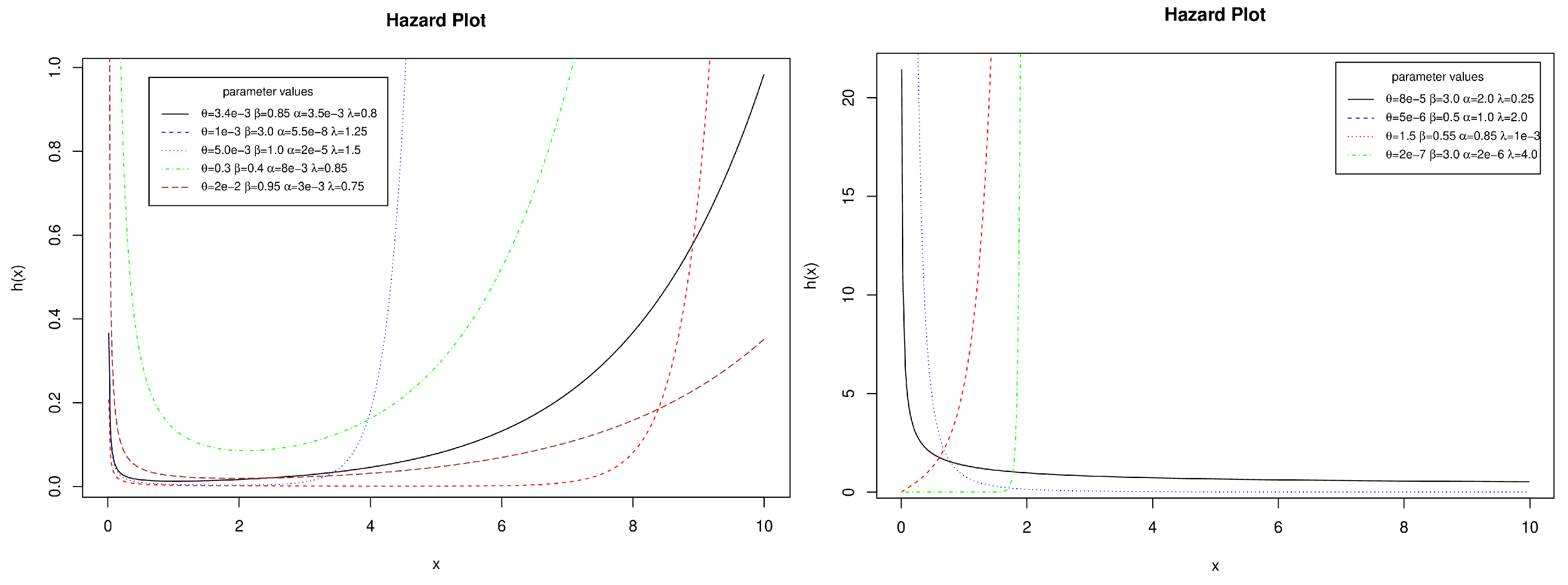
The behavior of the HRF of the FCD for some selected values can be seen in
Figure 1
As seen in
Figure 1, the FCD can model monotonic and non-monotonic behavior, establishing that the FCD is a flexible model to describe device lifetimes.
From Eq.
1, it is possible to obtain the Probability Density Function (PDF) of the FCD, which is described by:
The expression for the survival function
of FCP, as derived from Eq.
2, is presented as follows:
The estimation of the Cumulative Density Function (CDF) for the FCD, denoted as F(x), can be expressed as follows:
Additionally, The Cumulative Hazard Function
, from Eq. (
3) can be written as:
From Eq.
2 to
5 are valid in the reliability domain when
3. FCD Measures of Central Tendency
This section introduces certain statistical components that can enhance the reliability analysis.
3.1. Quantile
The
quantile q of the random variable
x for the FCD, derived from Eq.
4, can be expressed as:
Eq.
6 has no closed form, so obtaining FCD quantile values from numerical methods is possible.
3.2. FCD’s Mode
The FCD’s mode is determined by taking the first derivative of the PDF as defined in Eq.
2 and setting it to zero. Thus, the calculation of the FCD’s mode can be expressed as follows:
where
As in the quantile function, the mode does not have a closed form, so numerical methods must be used to estimate the mode of the FCD.
4. Moments and Incomplete Moments for FCD
This section presents the moments and incomplete moments with which it is possible to determine some aspects of quality in the devices under the reliability analysis, such as the Mean time between failures (MTTF), the variance, and other important metrics within the device analysis.
4.1. Moments
Theorem 1.
Consider a continuous random variable X with the FCD parameters . The moment of FCD with random variable X is expressed as:
where represents the gamma function.
Proof. The moment function can be calculated from the reliability equation
expressed in Eq.
3. Therefore, the moment function is expressed as:
Considering the S(x) of Eq.
3 and substituting it into Eq.
9 we have the following:
By establishing that:
Thus, the integral described in Eq.(
10) can be rewritten in the following way:
If the remaining integral is proposed to change the variable
, thus
y
.
Therefore:
Finally, using the definition of the
function, the result obtained can be found in Eq.(
8). □
4.2. Incomplete Moments
Theorem 2.
Let X be a continuous random variable with the FCD with . Then the incomplete moment of X can be expressed as follows:
Proof. The incomplete moments of any statistical distribution can be calculated as:
Hence,
taking into account the series expansion used in
Section 4.1:
The first part of the integral can be solved as:
The second part of the integral is solved by means of a change of variable
:
The last part of this integral can be expressed by means of
. And consequently, it is possible to arrive at the result of Eq.
11 □
5. Order Statistics
This section presents the order statistics of the FCD, which is used within reliability analyses to determine the performance of a device under analysis when said device has redundant systems. Generally, devices with redundant systems are used in critical operations.
Theorem 3.
Let be ordered statistics corresponding to a random sample of size n. let and be the pdf and cdf of FCD. Then, the pdf of order statistics is given by:
Proof. The order statistics of any distribution can be calculated as follows:
By substituting into Eq.(
2) and Eq. (
4) in Eq.(
13) we obtain:
By establishing the following expansions by series:
and by multiplying the exponential terms
It is possible to arrive at the result obtained in Eq.
12 □
6. Mean Residual Lifetime
One of the most important characteristics to determine within a device is to know what additional lifetime can be expected from a component when its lifetime has reached its limit; this is called mean residual lifetime (MRL).
Theorem 4.
The MRL for a device that is adjusted to the FCD presented in Eq.(2), is defined by:
Proof. Let X be a non-negative random variable, which represents the lifetime of a device with a survival function
that adjusts the CDF. Therefore, the MRL of said device under the FCD is described as:
By taking the
obtained in Eq.(
3) and substituting it in Eq.(
15), the following is obtained:
By recalling the series expansion carried out in
Section 4.1, the previous equation can be rewritten as follows:
To solve the remaining integral, let us consider a change of variable
,
,
and
the following is obtained:
The solution to the integral of the preceding equation can be obtained using the definition of the function
, leading to the outcome presented in Equation (
14). □
7. Entropy
Entropy within reliability analysis determines the uncertainty or randomness of the components within a system. However, it is also possible to characterize the fatigue damage of a device when it is in the final stages of its useful life.
7.1. Rényi Entropy
Proof. Let
X be a non-negative random variable with a PDF
. The Rényi Entropy of the order
p can be estimated as:
Considering the results derived from Eq. (
2) and incorporating them into Eq. (
17), we acquire.
First we develop
. To do this, we will consider the following series:
Rewriting the equation we have:
then, the resulting integral can be solved by a change of variable, which results in:
Finally, by applying the definition of the function
to the previous integral and by performing the corresponding algebra, it is possible to arrive at the result expressed in Eq.
16 □
8. Parameter Estimation of FCD
A crucial element of statistical distributions used in reliability analyses is estimating the parameters of the model with which the lifetimes are described. Therefore, two scenarios are proposed for the FCD to estimate the parameters. The first method addressed is the MLE, one of the most used methods for reliability analysis. The Bayesian analysis method is proposed, a robust technique for solving complex problems.
8.1. MLE for FCD
Let
be a random sample from the lifetime distribution with PDF
based on a sample of size m. Then the likelihood function of Eq. (
2) is written as follows:
By formulating the adobe equation, it is possible to express the log-likelihood function as follows:
The determination of the parameters
is specified in the following manner:
Conversely, starting from Eq.(
19) up to Eq.(
22), the Fisher information matrix can be constructed, facilitating the derivation of the Hessian. Further details about this matrix are provided in
Appendix A.
8.2. Bayesian Estimation for FCD
The Bayesian model is built from a specific prior distribution, which is denoted as
for
for the parameters of the model proposed in Eq.
2. In turn, to obtain the posterior distribution, it is necessary to multiply
given
by the likelihood function, which translates to:
where the likelihood function is given by:
For the FCD, we will assume that the parameters
are independent and that they follow a gamma distribution as a priori, that is,
and then:
By taking Eq.
24 and Eq.
25 and substituting them into Eq.
23, the posterior for the CDF can be written as:
As observed, the prior distributions for the FCD are influenced by certain parameters referred to as hyperparameters. In Bayesian analysis, these hyperparameters can either be assigned a prior value or estimated using the empirical Bayes approach. However, when following this approach, the analysis ceases to be fully Bayesian. Here, we choose hyperparameters for the gamma prior distributions in a way that their means approximate the maximum likelihood estimates (MLE) of the parameters in question, indicating that the MLEs play a role in shaping the prior information.
Thus, the estimation of the parameters
from a Bayesian perspective, are expressed as follows:
Due to the challenges in deriving mean parameter values analytically, employing techniques that simulate the posterior distribution becomes essential. Markov chain Monte Carlo (MCMC) methods are commonly applied for this purpose, with the Gibbs sampler and Metropolis algorithm being the most frequently used. However, these methods exhibit random walk behavior, which tends to be inefficient in exploring the target distribution, particularly in cases involving high-dimensional spaces or highly correlated parameters.
In this paper, Hamiltonian Monte Carlo (HMC) methods, specifically the No-U-Turn sampler variant, will be employed, whose main characteristic is that the parameters are adjusted as the algorithm performs computational iterations. This approach offers full Bayesian inference while eliminating the local random walk behavior and reducing sensitivity to correlated parameters seen in the Metropolis algorithm. As a result, it enables faster mixing and more efficient traversal through the target distribution.[
29].
Building on the previous discussion, let us make the following assumption. Suppose that
are generated from the posterior distribution defined by
. If ı is sufficiently large, i.e., greater than
, then
suggests a correlation between the sample and the true posterior. Furthermore, if we assume that convergence of the sampler requires running
m parallel chains, the means of the posterior distributions for the FCD parameters can be computed as follows:
To derive results from Eq.
27 to Eq. the PyMC package [
33] was used which was programmed in Python [
34]
9. Case of Study
This section tests the FCD in three case studies, with monotone and non-monotone behavior data. At the same time, a comparative analysis is proposed with other distributions formed with different methodologies to prove that the FCD offers competitive results. In turn, the following considerations are established in the case studies.
The data from the case studies do not consider censorship.
For estimating the parameters of each of the distributions of the comparative analysis, RStudio was used through the maxLik package [
35].
In the Bayesian inference, the following aspects were applied across all case studies: 10000 posterior samples with a Burn-In period of 1000 samples, three chains to assess parameter convergence, and three cores for parallel sampling.
To derive conclusions in each case study, the AIC, BIC are calculated. In turn, the Kolmogorov-Smirnov (K), Anderson-Darling (A), and Cramer Von Mises (CVM) tests, along with their P-values, are obtained to complement the analysis.
The distributions considered for the study cases are ChD, CWD, AddC, CPD, FrD, AWD, and FWD; the HF of each listed distribution is shown in
Table 1.
Table 1.
HRF of some recent Bathtub-shaped models used for all cases of study
Table 1.
HRF of some recent Bathtub-shaped models used for all cases of study
| Distribution |
|
| ChD |
|
| CWD |
|
| AddC |
|
| CPD |
|
| FrD |
|
| FWD |
|
| AWD |
|
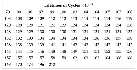
9.1. Case Study 1. Field-Tracking Study of a Larger System
In this case study, the data obtained Meeker et al. [
36] is considered, which analyzes the behavior of 30 devices inserted into the primary electrical system after a series of determined conditions and time had elapsed. The data obtained from said experiment can be seen in
Table 2.
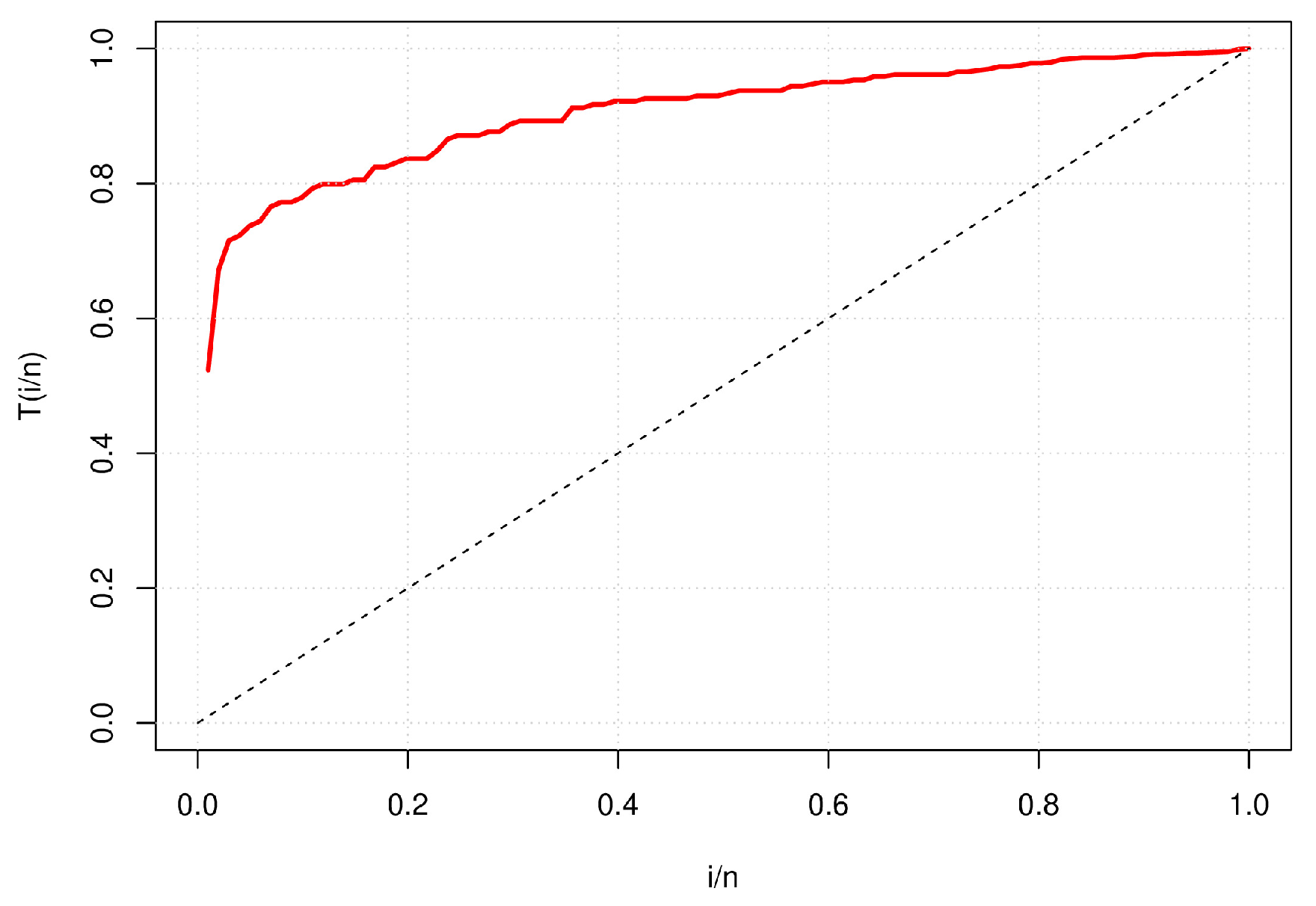
To identify what behavior the data established in
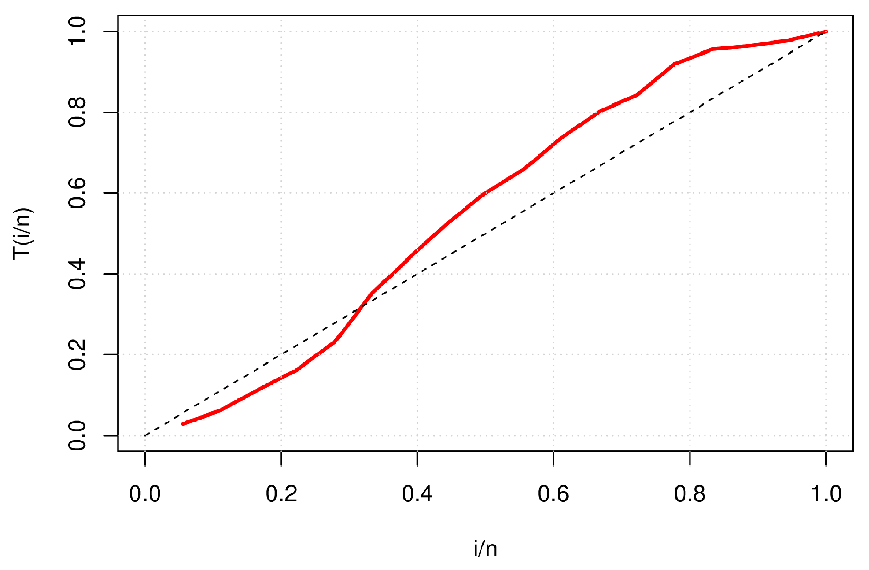
Table 2 follows, it is necessary to use the Time to Test Plot (TTT). Therefore,
Figure 2 presents the TTT plot of the case study 1.
The information is shown in
Figure 2 and based on what was established by Aarset [
37], the data in
Table 2 present a non-monotone behavior. Therefore, we estimate the parameters of each distribution established in
Table 1. The results of the estimations and the statistics are presented in
Table 3.
The values of the parameters presented in
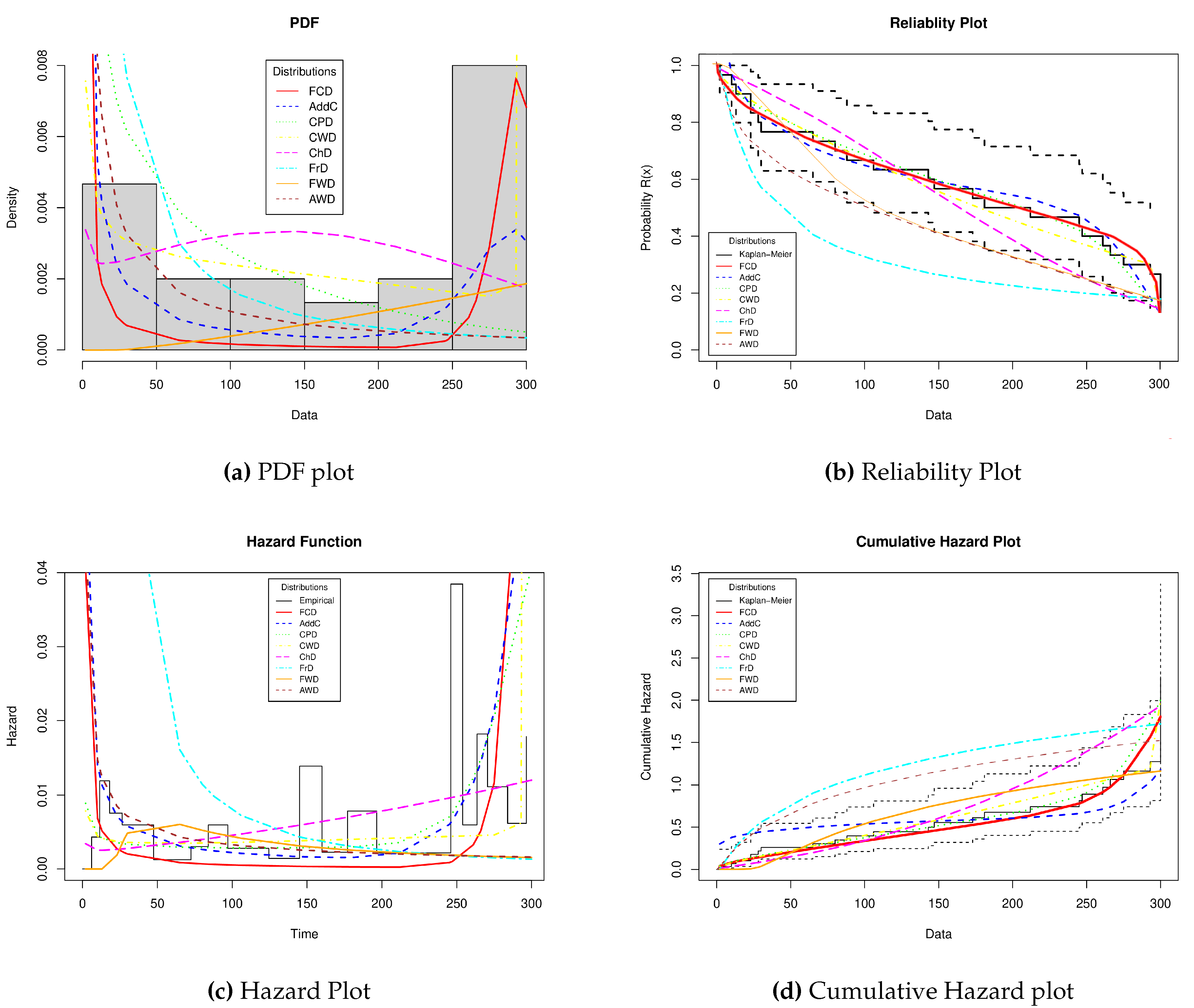
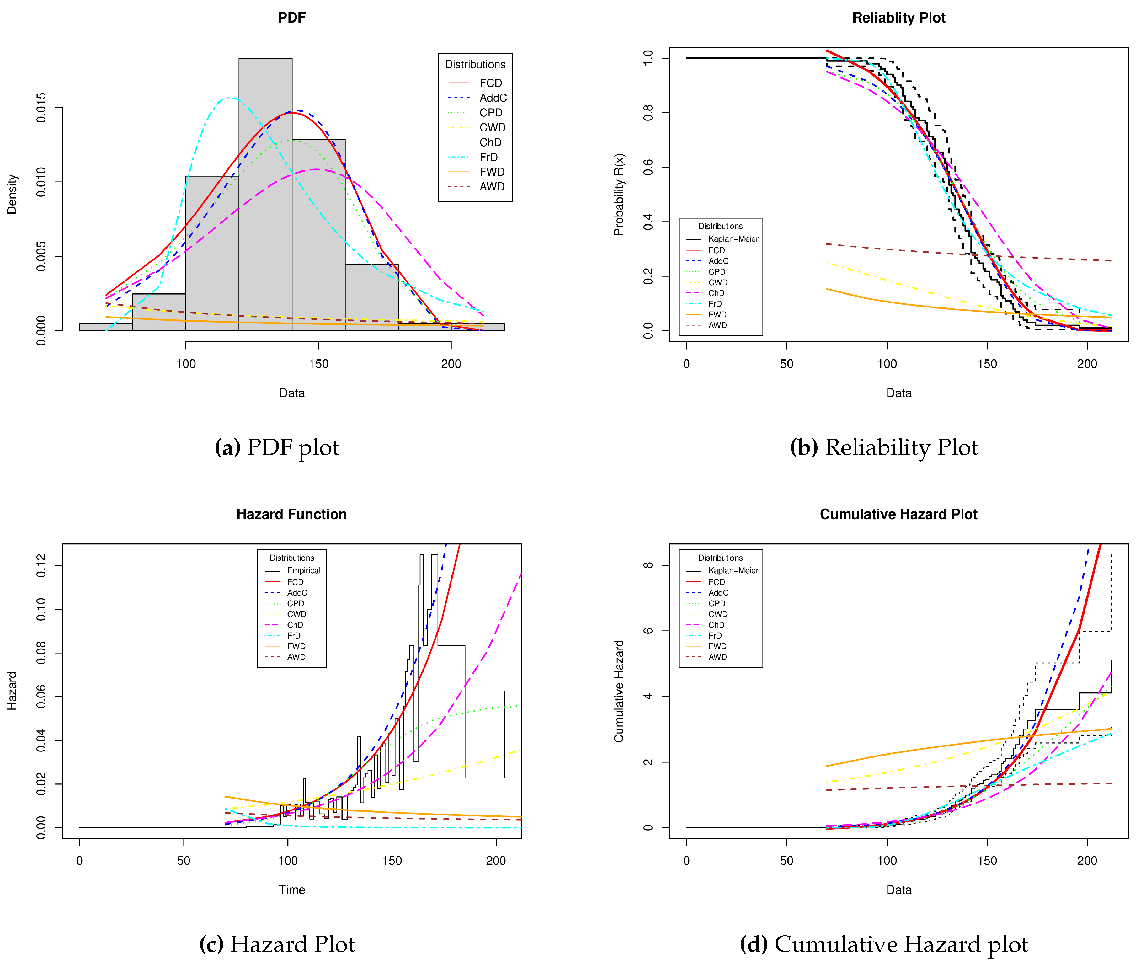
Table 3 show that the FCD offers very competitive results concerning other distributions with similar properties and that the base distributions of the FCD. This statement is supported by the K-S, A, and W statistics with the respective P-values obtained for each distribution. On the other hand, the graphical representations of PDF, Reliability, Hazard, and Cumulative Hazard are presented in
Figure 3
As can be seen in
Figure 3, the behavior of the FCD concerning the data histogram is competitive; however, the AddC also presents a good fit; this can be verified with the statistics in
Table 3 where both distributions offer similar results. At the same time, in
Figure 3, you can see the reliability graph, where the behavior of the distributions concerning the Kaplan-Meier empirical reliability (confidence intervals are shown on the dotted line) is established. Likewise, it can be seen that the FCD describes very closely the behavior of the real devices against the values that are estimated empirically, which is an indication that the FCD estimated the MTTF values and warranty times, which can be attractive to practitioners.
Figure 3 shows the representation of the failures of the devices under analysis concerning their empirical behavior and the forms the distributions under analysis take. In this case, the FCD, the AddC, CPD, and CWD offer non-monotonic representations, as shown by the TTT plot in
Figure 2. However, the FCD touches on more points to the empirical representation and has a shape similar to the bathtub curve. This shape of the FCD indicates that practitioners can determine maintenance times closer to the actual behavior of the device. Finally, in
Figure 3, the Cumulative Hazard plot is shown, where the empirical behavior is established along with the confidence intervals. In this case, the FCD shows very good results. This capacity is shown by the newly proposed distribution, which more closely models the failures of the device as its useful life passes.
An algorithm based on HMC was implemented to obtain the Bayes estimation and the reliability characteristics. For this purpose, the configuration was established at the beginning of section 9.
The results of the Bayes estimations for the parameters
, and
are shown in
Table 4, where they are also compared with the results obtained by the MLE of the distribution under analysis. The results show that the parameters are close in both cases.
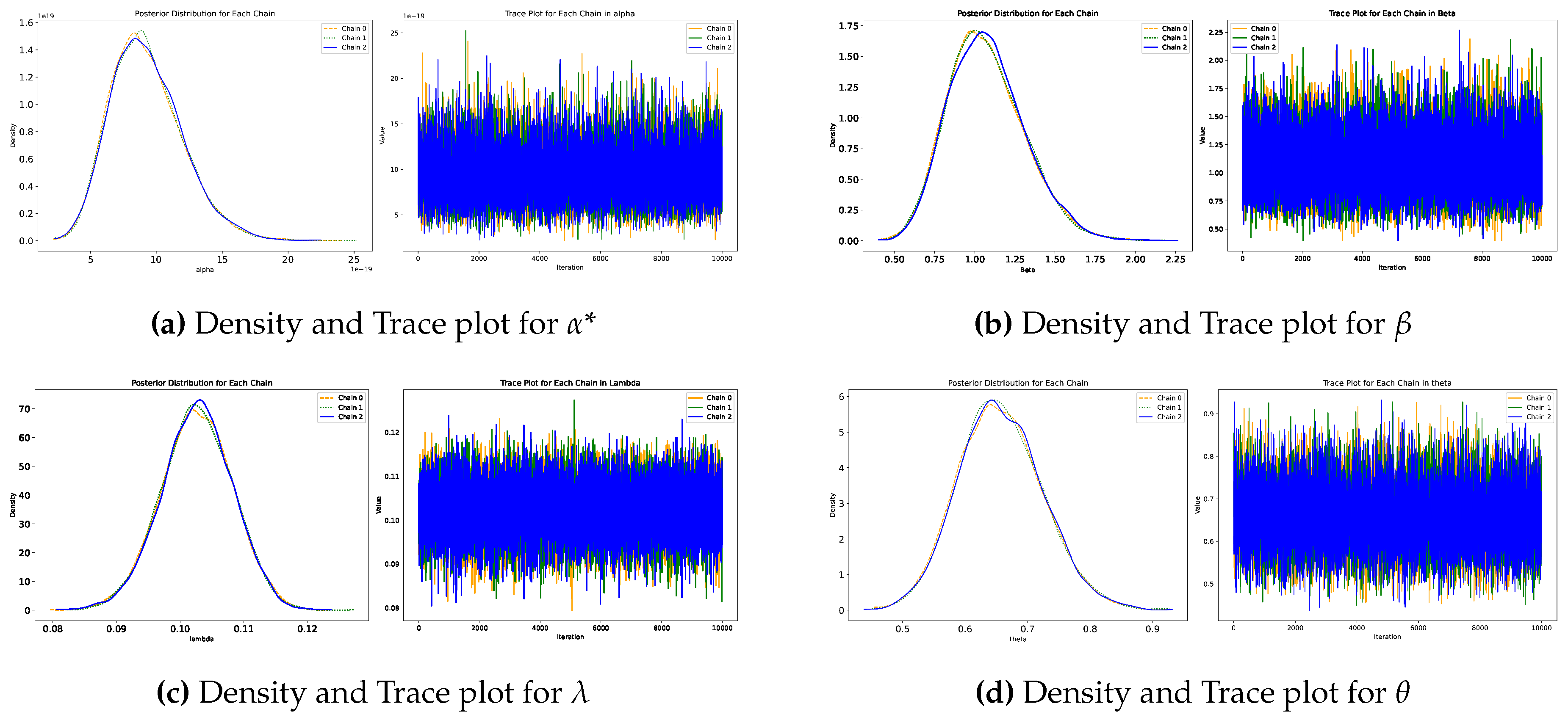
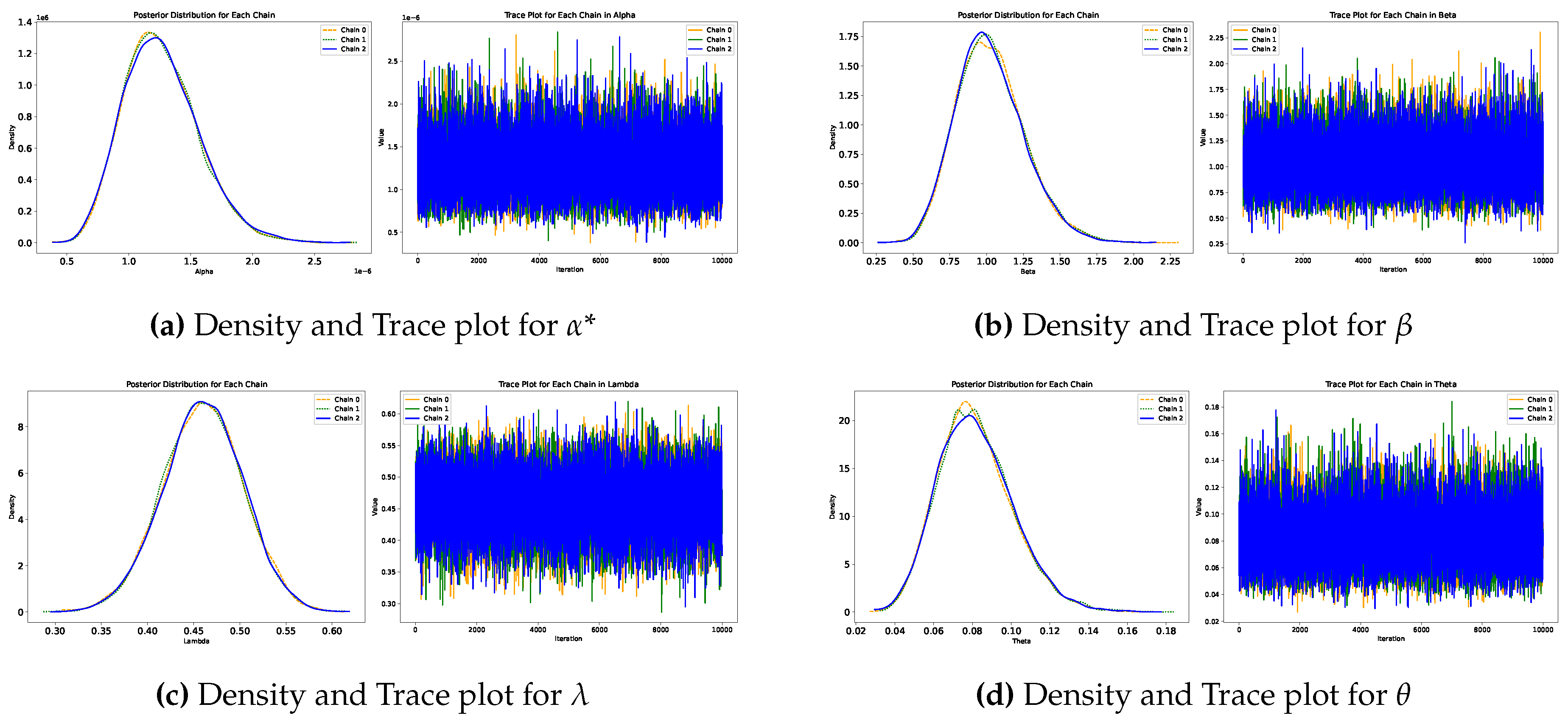
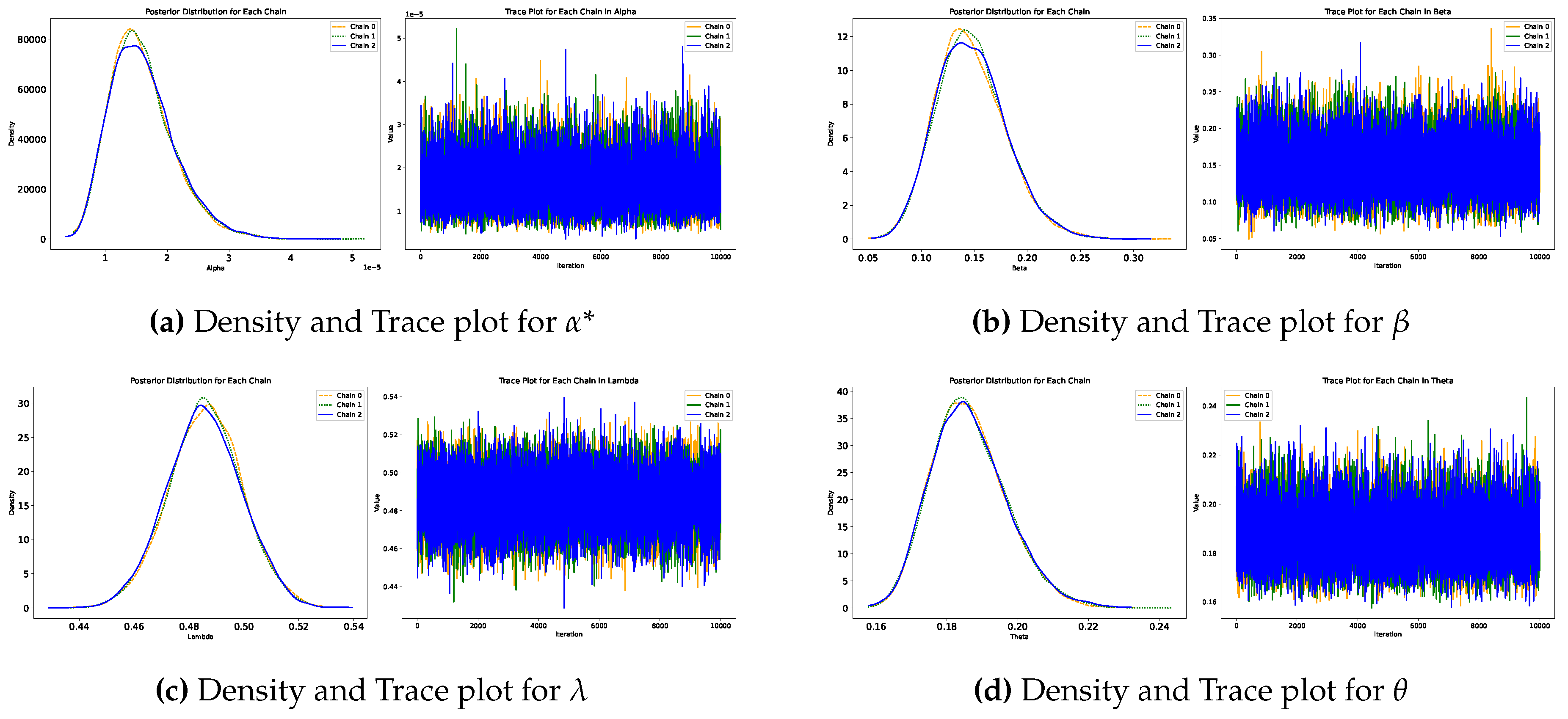
Figure 4 presents the trace plots and estimated densities for each parameter as derived from the HMC algorithm. The trace plots illustrate the parallel chains used in the simulation, demonstrating that convergence has been achieved for each parameter. The densities are roughly symmetrically distributed around their central values, indicating that they offer reliable Bayesian estimates.
9.2. Case Study 2. Evaluation of the Reliability of Eighteen Electronic Gadgets
In this case study, the lifetimes of eighteen electronic devices are examined, with the data provided by Wang [
38]. The failure times are detailed in
Table 5. In turn,
Figure 5 illustrates the behavior of the TTT plot for the data shown in
Table 5.
Table 6 presents the parameter estimates for case study 2. This table shows that the FCD delivers highly competitive results compared to the distributions in
Table 2. This finding is supported by the statistical values obtained from assessing each distribution’s performance concerning lifetimes. Ultimately, the reliability graph behavior can be inferred from the results in
Table 5, with these graphs illustrated in
Figure 5.
The reliability graphs in
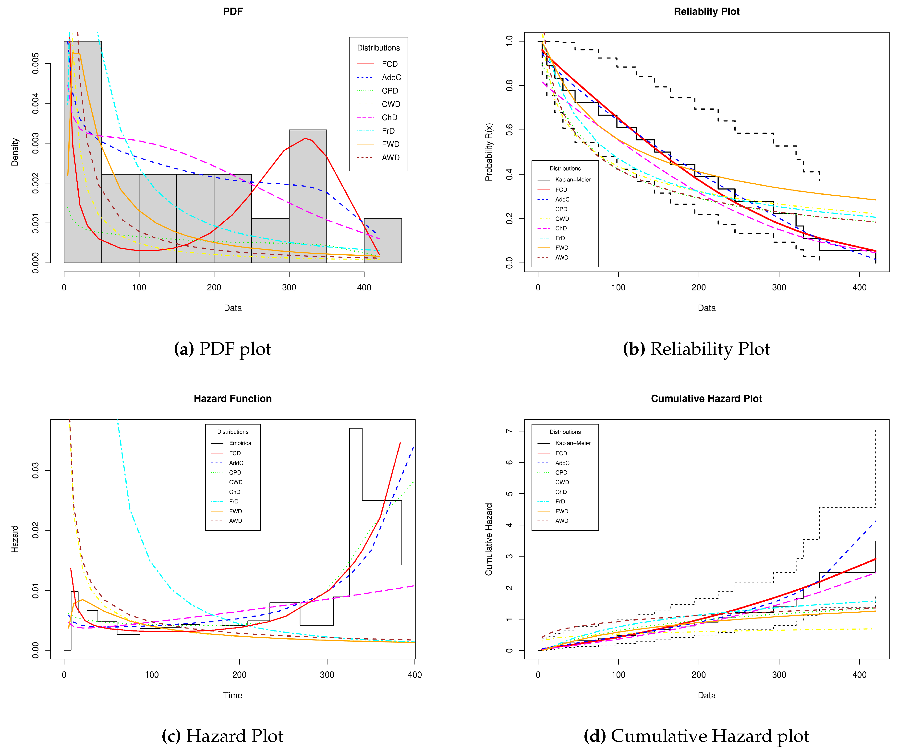
Figure 6 present intriguing insights into how the data behaves under the various distributions analyzed. In
Figure 6, the various patterns of the data from
Table 6 are depicted concerning each of the PDFs used in the comparative study. The FCD appears to fit the histogram of lifetimes well, with AddC and ChD following closely behind in terms of fit. The reliability graph in
Figure 6 confirms that the FCD closely aligns with the empirical reliability data obtained from the Kaplan-Meier estimate. This suggests that the FCD accurately reflects the device’s performance under field conditions. Additionally, this fit allows manufacturers to develop warranty plans that are more closely aligned with the actual behavior of the device.
Figure 6 illustrates the relationship between lifetimes and the hazard function. It is evident that both the FCD and AddC models align well with the empirical data. Nevertheless, the FCD model intersects the empirical trajectory at more points, a finding that is corroborated by the statistics presented in
Table 6. Finally,
Figure 6 presents the Cumulative Hazard plot, showing the empirical data and its confidence intervals. In this plot, the FCD demonstrates excellent performance. This effectiveness is highlighted by the new distribution, which more accurately models device failures as their useful life advances.
Table 7 presents the estimates derived from the Bayesian method, comparing the parameters of the FCD with those obtained from the MLE. The results indicate that the parameters from both approaches yield similar values.
Figure 7 presents the densities and traces generated using HMC for each parameter of the FCD in case study 2. The results indicate that the simulations converge to the same target distribution, and it is evident that the estimated densities for each parameter are roughly symmetrical around the central values.
9.3. Case Study 3. Fatigue Time Data
This case study provides details on the endurance limit of 6061-T6 aluminum samples, which were cut parallel to the rolling direction and subjected to oscillation at a frequency of 18 cycles per second and a maximum stress of 31,000 psi, as reported by Birnbaum and Saunders [
39]. Experimental data is presented in
Table 8.
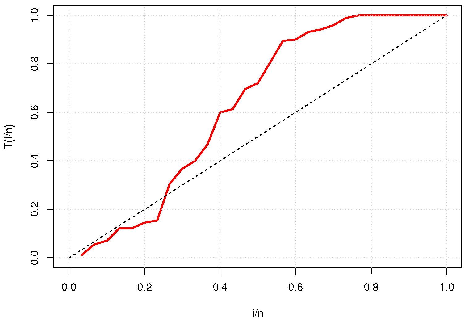
Figure 6 offers an empirical depiction of this data via the TTT plot, revealing that the data in
Table 8 exhibit a consistently increasing trend. Based on this evidence, parameters were estimated for each distribution, with the results summarized in
Table 9.
Table 8.
Lifetimes of 6061-T6 aluminum samples presented by Birnbaum and Saunders
Table 8.
Lifetimes of 6061-T6 aluminum samples presented by Birnbaum and Saunders
Figure 8.
TTT plot for Data presented in
Table 8.
Figure 8.
TTT plot for Data presented in
Table 8.
Table 9 shows the values of the estimates for case study 3. As for non-monotone failure times, the FCD shows a good adjustment to failure times with monotone behavior. This statement is supported by the results of the FCD statistics and its competing distributions. This statement demonstrates that the FCD has great flexibility in representing the lifetimes of different classes of devices and that it may prove to be a viable option for reliability engineering practitioners. On the other hand,
Figure 9 shows the reliability graphs for case study 3 obtained from the values of the parameters estimated in
Table 9.
Figure 9a shows the shape the PDFs take for each distribution under analysis. For this case, we can observe that the FCD, AddC, CPD, ChD, and FrD stand out in how they fit the histogram of the data, which may indicate candidates who represent the failure times of the devices under analysis. On the other hand, CWD, FWD, and AWD, despite having the flexibility to represent monotone and non-monotone data, are not capable of following the shape of the histogram; this is reflected in the poor results obtained in the statistics presented in
Table 9.
Figure 9b shows the behavior of the pieces under analysis when they are analyzed using the different methodologies. In this graph, it is worth noting that the FCD shows a better fit concerning empirical reliability and the limits marked with the dotted lines. Nevertheless, it is worth highlighting the behavior of the AddC, CPD, ChD, and FrD, which are close. However, in some cases, their representation goes outside the established limits, so practitioners could opt for the FCD to estimate warranty and maintenance. Concerning the hazard plot shown in
Figure 9, it can be seen that the data have an increasing monotone behavior. At this point, only the FCD, AddC, and the ChD show a behavior similar to that established by the empirical representation. However, when considering the statistics obtained in
Table 9, it establishes that the FCD is the best option to describe the life of the device throughout its useful life. Finally,
Figure 9 presents the behavior of the Cumulative Hazard plot, with which the risk of an event occurring at a given time is measured, given that the event has not occurred before. In this case, the FCD shows touching the empirical accumulated failures in a greater number of points. However, the AddC shows very competitive results, but considering that this graph measures the median survival time and the mean survival time, the FCD may turn out to be the best option in practice.
On the other hand,
Table 10 compares the estimated values for each parameter of the FCD under MLE and the Bayesian analysis following the data established in
Table 8. In the case of data with a monotonic behavior, the FCD shows that the values of each parameter are similar under the two estimation approaches, indicating that the proposed distribution offers very competitive results.
Finally,
Figure 10 illustrates the density shape and traces from each simulation chain for the parameters in case study 3. Similar to the previous two cases, the simulations converge around the mean values of the estimated parameters, with the densities for each parameter showing a strong symmetry around these estimated values.
10. Conclusion and Future Work
This paper introduces a novel distribution for analyzing lifetimes derived from reliability engineering techniques. The new distribution was developed using an additive methodology, incorporating the hazard functions of both the Chen Distribution and the Fréchet Distribution. As a result of the proposed methodology, a four-parameter FCD was developed, consisting of three shape parameters and one scale parameter. Additionally, the paper presents key statistical properties related to lifetimes, enabling practitioners to consider the FCD as a viable option for modeling the behavior of electrical and mechanical devices, among others. One of the FCD’s standout features is its ability to yield competitive results compared to other distributions that effectively model monotone and non-monotone data (such as those represented by the bathtub curve). These representations are crucial for understanding device performance over its useful life. The paper proposes equations derived from the MLE and Bayesian methods to estimate the FCD parameters. These methods were implemented in RStudio and Python, making the distribution more appealing to practitioners using either estimation approach.
This new distribution has been evaluated through three case studies focused on the lifetime characteristics of electronic devices. In these studies, scenarios were examined where lifetimes exhibited monotonic and non-monotonic failure behaviors, demonstrating the FCD’s adaptability to the various types of data electronic devices may produce during reliability testing. The results indicate that the FCD delivers highly competitive performance compared to other distributions with similar characteristics, making it a strong option for reliability practitioners when selecting a distribution to describe lifetimes. Additionally, results from the two most widely used parameter estimation methods, MLE and Bayesian Analysis, have been presented. In all case studies, the estimates from both approaches were very similar, reinforcing the practicality of this new distribution.
The uses of this new distribution extend beyond reliability analysis; the FCD can also model datasets in fields like actuarial science to assess an individual’s risk and in medical statistics to analyze mortality rates among patients with a particular disease.
In conclusion, future work could modify the FCD by introducing an additional exponential parameter, enhancing its applicability and adaptability for modeling various real-world datasets. Additionally, estimates of the FCD parameters could be derived using a neural network, allowing for comparison with MLE and Bayesian methods.
Author Contributions
Conceptualization, L.C.M.-G.; methodology, L.C.M.-G.; validation, L.A.R.-P. and I.J.C.P.-O.; data curation, L.A.R.-P. and I.J.C.P.-O.; formal analysis, L.C.M.-G. and L.A.R.-P.; investigation, L.C.M.-G. and I.J.G.H.; supervision, L.C.M.-G. and A.E.Q.C.; resources, L.C.M.-G.; writing—original draft preparation, L.C.M.-G.; writing—review and editing, L.A.R.-P., I.J.C.P.-O. and I.J.G.H..; visualization, L.A.R.-P., I.J.C.P.-O. and A.E.Q.C. All authors have read and agreed to the published version of the manuscript.
Conflicts of Interest
Declare conflicts of interest or state “The authors declare no conflicts of interest.” Authors must identify and declare any personal circumstances or interest that may be perceived as inappropriately influencing the representation or interpretation of reported research results. Any role of the funders in the design of the study; in the collection, analyses or interpretation of data; in the writing of the manuscript; or in the decision to publish the results must be declared in this section. If there is no role, please state “The funders had no role in the design of the study; in the collection, analyses, or interpretation of data; in the writing of the manuscript; or in the decision to publish the results”.
Appendix A. Fisher Information Matrix
The Fisher Information Matrix is formed from the following:
References
- Al-Essa, L.A.; Muhammad, M.; Tahir, M.; Abba, B.; Xiao, J.; Jamal, F. A new flexible four parameter bathtub curve failure rate model, and its application to right-censored data. IEEE Access 2023. [Google Scholar] [CrossRef]
- Mahdavi, A.; Kundu, D. A new method for generating distributions with an application to exponential distribution. Communications in Statistics-Theory and Methods 2017, 46, 6543–6557. [Google Scholar] [CrossRef]
- Kumar, D.; Singh, U.; Singh, S.K. A method of proposing new distribution and its application to Bladder cancer patients data. J. Stat. Appl. Pro. Lett 2015, 2, 235–245. [Google Scholar]
- Maurya, S.; Kaushik, A.; Singh, S.; Singh, U. A new class of distribution having decreasing, increasing, and bathtub-shaped failure rate. Communications in Statistics-Theory and Methods 2017, 46, 10359–10372. [Google Scholar] [CrossRef]
- Shama, M.S.; El Ktaibi, F.; Al Abbasi, J.N.; Chesneau, C.; Afify, A.Z. Complete Study of an Original Power-Exponential Transformation Approach for Generalizing Probability Distributions. Axioms 2023, 12, 67. [Google Scholar] [CrossRef]
- Mead, M.E.; Cordeiro, G.M.; Afify, A.Z.; Al Mofleh, H. The alpha power transformation family: properties and applications. Pakistan Journal of Statistics and Operation Research 2019, 525–545. [Google Scholar] [CrossRef]
- Dey, S.; Nassar, M.; Kumar, D.; Alzaatreh, A.; Tahir, M.H. A new lifetime distribution with decreasing and upside-down bathtub-shaped hazard rate function. Statistica 2019, 79, 399–426. [Google Scholar]
- Deepthi, K.; Chacko, V. An upside-down bathtub-shaped failure rate model using a DUS transformation of lomax distribution. In Stochastic models in reliability engineering; CRC Press, 2020; pp. 81–100. [CrossRef]
- Ahsan-ul Haq, M.; Aldahlan, M.A.; Zafar, J.; Gómez, H.W.; Afify, A.Z.; Mahran, H.A. A new cubic transmuted power-function distribution: Properties, inference, and applications. Plos one 2023, 18, 1–15. [Google Scholar] [CrossRef] [PubMed]
- Lai, C.; Xie, M.; Murthy, D. A modified Weibull distribution. IEEE Transactions on reliability 2003, 52, 33–37. [Google Scholar] [CrossRef]
- Shama, M.S.; Alharthi, A.S.; Almulhim, F.A.; Gemeay, A.M.; Meraou, M.A.; Mustafa, M.S.; Hussam, E.; Aljohani, H.M. Modified generalized Weibull distribution: theory and applications. Scientific Reports 2023, 13, 12828. [Google Scholar] [CrossRef] [PubMed]
- Lemonte, A.J. A new exponential-type distribution with constant, decreasing, increasing, upside-down bathtub and bathtub-shaped failure rate function. Computational Statistics & Data Analysis 2013, 62, 149–170. [Google Scholar]
- Sarhan, A.M.; Zaindin, M. Modified Weibull distribution. APPS. Applied Sciences 2009, 11, 123–136. [Google Scholar]
- Khalil, A.; Ijaz, M.; Ali, K.; Mashwani, W.K.; Shafiq, M.; Kumam, P.; Kumam, W. A novel flexible additive Weibull distribution with real-life applications. Communications in Statistics-Theory and Methods 2021, 50, 1557–1572. [Google Scholar] [CrossRef]
- Wang, L.; Wu, K.; Tripathi, Y.M.; Lodhi, C. Reliability analysis of multicomponent stress–strength reliability from a bathtub-shaped distribution. Journal of Applied Statistics 2022, 49, 122–142. [Google Scholar] [CrossRef] [PubMed]
- Ghazal, M. A new extension of the modified Weibull distribution with applications for engineering data. Probabilistic Engineering Mechanics 2023, 74, 103523. [Google Scholar] [CrossRef]
- Xie, M.; Tang, Y.; Goh, T.N. A modified Weibull extension with bathtub-shaped failure rate function. Reliability Engineering & System Safety 2002, 76, 279–285. [Google Scholar]
- Thach, T.T. A three-component additive weibull distribution and its reliability implications. Symmetry 2022, 14, 1455. [Google Scholar] [CrossRef]
- Sharma, V.K.; Singh, S.V.; Chesneau, C. A Family of Additive Teissier–Weibull Hazard Distributions for Modeling Bathtub-Shaped Failure Time Data. International Journal of Reliability, Quality and Safety Engineering 2023, 30, 2350003. [Google Scholar] [CrossRef]
- Jha, V.; Kumaran, V. The Exponentiated Additive Teissier-Exponential Distribution. Lobachevskii Journal of Mathematics 2023, 44, 3697–3713. [Google Scholar] [CrossRef]
- Abd EL-Baset, A.A.; Ghazal, M. Exponentiated additive Weibull distribution. Reliability Engineering & System Safety 2020, 193, 106663. [Google Scholar]
- Xavier, T.; Jose, J.K.; Nadarajah, S. An additive power-transformed half-logistic model and its applications in reliability. Quality and Reliability Engineering International 2022, 38, 3179–3196. [Google Scholar] [CrossRef]
- Kotz, S.; Nadarajah, S. Extreme value distributions: theory and applications; world scientific, 2000. [CrossRef]
- Baharith, L.A. A new generalization of the exponentiated Frechet distribution with applications. Journal of Reliability and Statistical Studies 2022, 129–152. [Google Scholar] [CrossRef]
- Zayed, M.; Butt, N.S. The extended Fréchet distribution: Properties and applications. Pakistan Journal of Statistics and Operation Research 2017, 529–543. [Google Scholar] [CrossRef]
- Deka, D.; Das, B.; Baruah, B.K.; Baruah, B. Some properties on Fréchet-Weibull distribution with application to real life data. Math Stat 2021, 9, 8–15. [Google Scholar] [CrossRef]
- Alzawq, F.S.A.; ElKholy, A.K. Pak. J. Statist. 2023 Vol. 39 (3), 387-414 THE GENERALIZED FRÉCHET DISTRIBUTION WITH VARIABLE HAZARD RATE SHAPES: PROPERTIES AND APPLICATIONS. Pak. J. Statist 2023, 39, 387–414. [Google Scholar]
- Chen, Z. A new two-parameter lifetime distribution with bathtub shape or increasing failure rate function. Statistics & Probability Letters 2000, 49, 155–161. [Google Scholar]
- Thanh Thach, T.; Briš, R. An additive Chen-Weibull distribution and its applications in reliability modeling. Quality and Reliability Engineering International 2021, 37, 352–373. [Google Scholar] [CrossRef]
- Khan, M.S.; King, R.; Hudson, I.L. Transmuted exponentiated Chen distribution with application to survival data. ANZIAM Journal 2015, 57, C268–C290. [Google Scholar] [CrossRef]
- Méndez-González, L.C.; Rodríguez-Picón, L.A.; Rodríguez Borbón, M.I.; Sohn, H. The Chen–Perks Distribution: Properties and Reliability Applications. Mathematics 2023, 11, 3001. [Google Scholar] [CrossRef]
- Méndez-González, L.C.; Rodríguez-Picón, L.A.; Pérez-Olguín, I.J.C.; Vidal Portilla, L.R. An additive chen distribution with applications to lifetime data. Axioms 2023, 12, 118. [Google Scholar] [CrossRef]
- Abril-Pla, O.; Andreani, V.; Carroll, C.; Dong, L.; Fonnesbeck, C.J.; Kochurov, M.; Kumar, R.; Lao, J.; Luhmann, C.C.; Martin, O.A.; others. PyMC: a modern, and comprehensive probabilistic programming framework in Python. PeerJ Computer Science 2023, 9, e1516. [Google Scholar] [CrossRef] [PubMed]
- Van Rossum, G.; Drake, F.L. Python 3 Reference Manual; CreateSpace: Scotts Valley, CA, 2009. [Google Scholar]
- Henningsen, A. MaxLik: An R Package for Maximum Likelihood Estimation. Journal of Statistical Software 2011, 39, 1–25. [Google Scholar] [CrossRef]
- Meeker, W.Q.; Escobar, L.A.; Pascual, F.G. Statistical methods for reliability data; John Wiley & Sons, 2021.
- Aarset, M.V. How to identify a bathtub hazard rate. IEEE Transactions on Reliability 1987, 36, 106–108. [Google Scholar] [CrossRef]
- Wang, F.K. A new model with bathtub-shaped failure rate using an additive Burr XII distribution. Reliability Engineering & System Safety 2000, 70, 305–312. [Google Scholar]
- Birnbaum, Z.W.; Saunders, S.C. Estimation for a family of life distributions with applications to fatigue. Journal of applied probability 1969, 6, 328–347. [Google Scholar] [CrossRef]
|
Disclaimer/Publisher’s Note: The statements, opinions and data contained in all publications are solely those of the individual author(s) and contributor(s) and not of MDPI and/or the editor(s). MDPI and/or the editor(s) disclaim responsibility for any injury to people or property resulting from any ideas, methods, instructions or products referred to in the content. |
© 2024 by the authors. Licensee MDPI, Basel, Switzerland. This article is an open access article distributed under the terms and conditions of the Creative Commons Attribution (CC BY) license (http://creativecommons.org/licenses/by/4.0/).
