Identification and Quantification of Hidden Dangers in Small Scale Reservoir Engineering Based on Deep Learning for Flood control, water supply and irrigation

This study aims to enhance the detection and assessment of safety hazards in small-scale reservoir engineering using advanced image processing and deep learning techniques. Given the critical importance of small reservoirs in flood management, water supply, and ecological balance, the effective monitoring of their structural integrity is crucial. This paper developed a fully convolutional semantic segmentation method for hidden danger images of small reservoirs using an encoding-decoding structure, utilizing a deep learning framework of convolutional neural networks (CNNs) to process and analyze high-resolution images captured by UAVs. The method incorporated data augmentation and adaptive learning techniques to improve model accuracy under diverse environmental conditions. Finally, the quantification data of hidden dangers (length, width, area, etc.) was obtained by converting the image pixels to the actual size. Results demonstrate significant improvements in detecting structural deficiencies, such as cracks and seepage areas, with increased precision and recall rates compared to conventional methods, and the HHSN-25 network (Hidden Hazard Segmentation Network with 25 layers)proposed in this paper outperforms other methods. The main evaluation indicator mIoU of HHSN-25 is higher than other methods, reaching 87.00%, and Unet is 85.50%, Unet++is 85.55%. The proposed model achieves reliable real-time performance, allowing for early warning and effective management of potential risks. This study contributes to the development of more efficient monitoring systems for small-scale reservoirs, enhancing their safety and operational sustainability.

Keywords:

Subject: Engineering - Safety, Risk, Reliability and Quality

1. Introduction

Small-scale reservoirs are a critical component of water resource management and play an essential role in flood control, irrigation, and ecological preservation, particularly in regions susceptible to climatic and hydrological variability [1]. In China alone, there are over 98,000 reservoirs, of which 95% are classified as small-scale, reflecting their pivotal importance in the national context. Among these, Jiangxi Province is particularly notable, with over 10,300 small-scale reservoirs—accounting for 11.4% of the country’s total [2]. These reservoirs significantly contribute to the socio-economic development of the region by mitigating floods, ensuring agricultural productivity, and maintaining ecological balance. However, the safety and stability of these small-scale reservoirs remain a significant challenge due to several factors, including inadequate design, incomplete hydrological and geological data, and substandard construction practices. These challenges render small-scale reservoirs more susceptible to failures compared to their larger counterparts [3,4]. The monitoring and assessment of small-scale reservoirs have traditionally relied on manual inspections and conventional surveillance methods. These approaches are not only labor-intensive and time-consuming but also prone to human error, which can compromise the timely detection of hazards [5,6,7]. Consequently, there is an increasing demand for automated and accurate techniques that can enhance the safety management of small-scale reservoirs. One promising solution is the application of image processing and machine learning techniques, particularly deep learning, to the detection and characterization of structural defects in reservoirs [8].

The conventional approaches to reservoir safety monitoring, such as visual inspections, geotechnical instrumentation, and satellite remote sensing, have provided essential baseline data for hazard detection and management. However, these methods exhibit several limitations. Visual inspections and manual monitoring are labor-intensive, limited by human capability, and can be subjective and inconsistent [9]. Geotechnical instrumentation provides detailed point-based measurements but lacks spatial coverage and can be affected by external environmental factors [10]. Satellite remote sensing offers wide-area coverage but is often hindered by coarse resolution, low revisit frequency, and sensitivity to atmospheric conditions [11]. In recent years, several studies have explored the potential of machine learning techniques, such as support vector machines (SVM) and random forests, for detecting and classifying structural anomalies in large dams [12]. These methods, while promising, have not yet been extensively applied to small-scale reservoirs. The specific challenges of small-scale reservoirs, such as their varied construction standards, diverse environmental settings, and unique hydrological conditions, necessitate the development of more tailored and sophisticated monitoring techniques [13,14].

Deep learning, particularly convolutional neural networks (CNNs), has emerged as a powerful tool for image-based structural defect detection due to its ability to automatically learn and extract hierarchical features from complex datasets [15]. CNN-based methods have been successfully applied in various fields, including urban infrastructure monitoring [16], crack detection in concrete surfaces [17], and landslide mapping [18]. These studies demonstrate that deep learning models, especially when combined with high-resolution imagery, can provide detailed and accurate assessments of structural conditions. Semantic segmentation, a subfield of deep learning, has proven particularly effective in detecting and categorizing structural defects in various settings [19]. Unlike traditional image classification, which assigns a single label to an entire image, semantic segmentation provides pixel-wise classification, enabling precise localization and characterization of defects [20]. This capability is crucial for identifying and analyzing multiple types of hazards in small-scale reservoirs, where defects may vary significantly in size, shape, and context [21]. While there have been significant advancements in the application of deep learning for infrastructure monitoring, most studies have focused on large-scale structures or urban environments. There is a noticeable gap in the application of these technologies to small-scale reservoirs, which are characterized by unique hazard patterns that differ significantly in spatial scale and temporal dynamics from those of larger infrastructure [22]. Furthermore, the integration of deep learning models with multi-source data, such as hydrological, geological, and meteorological data, for comprehensive risk assessment and prediction remains underexplored [23].

This study aims to bridge this gap by developing a novel semantic segmentation-based framework for small-scale reservoir safety monitoring. The proposed framework utilizes a combination of deep learning techniques and multi-source data fusion to achieve quantitative extraction of key warning indicators, such as cracks, seepage areas, and surface deformation. This approach integrates image data with conventional monitoring datasets to establish a robust model for real-time hazard evaluation and prediction, enhancing early warning capabilities and operational safety [24]. Our approach involves the development of a deep learning model based on semantic segmentation to identify and categorize various types of structural hazards in small-scale reservoirs. This model leverages multi-source data, including UAV imagery, multispectral and infrared data, and environmental sensor data, to capture the diverse range of hazard indicators present in reservoir environments [25]. We utilize a U-Net architecture, a popular choice in semantic segmentation tasks, due to its ability to retain fine spatial details while capturing global contextual information [26]. To enhance the robustness and accuracy of the model, we integrate domain adaptation techniques to handle the variability in data quality and environmental conditions. Furthermore, we employ data augmentation strategies, such as random cropping, flipping, and brightness adjustment, to increase the diversity of the training data and improve model generalization.

The proposed framework offers several significant contributions to the field of reservoir safety monitoring. First, it provides a comprehensive methodology for the automatic detection and classification of structural hazards in small-scale reservoirs, addressing a critical gap in current research. Second, by integrating multi-source data, our approach enables a more holistic assessment of reservoir safety, capturing a broader range of hazard indicators and providing more accurate predictions of potential failures. Moreover, the development of a real-time hazard evaluation and prediction model has practical implications for improving the operational safety of small-scale reservoirs. The ability to detect and respond to hazards promptly can significantly reduce the risk of failure, minimize damage, and ensure the continued provision of essential water services. This is particularly relevant in regions such as Jiangxi Province, where small-scale reservoirs play a critical role in supporting socio-economic development and maintaining ecological balance. By leveraging semantic segmentation techniques and multi-source data fusion, we aim to provide a more accurate and comprehensive assessment of reservoir safety, enhancing early warning capabilities and contributing to the sustainable management of water resources. This research not only addresses existing gaps in the literature but also offers a practical solution to the challenges faced by small-scale reservoir engineering in China and beyond.

2. Construction of Hidden Hazards Dataset for Small Reservoir Engineering

2.1. Causes of Hidden Hazards in Small-Scale Reservoirs

Small-scale reservoirs, as a critical component of water resource management, have various causes of safety hazards. These mainly involve the following aspects:

Design and Construction Deficiencies: Many small-scale reservoirs lack standardization in their initial design and construction stages, especially those built during the mid-20th century's large-scale construction efforts. Common issues include non-standardized design, poor-quality construction materials, and outdated construction techniques. These factors make the reservoirs susceptible to structural damage over time or under extreme weather conditions, leading to potential hazards such as dam cracks, seepage, and landslides.

Material and Structural Issues: The construction of small-scale reservoirs often relies on locally available materials, which may not meet durability and stability standards. Additionally, the aging and erosion of dam structures exacerbate material deterioration, triggering hazards. For instance, earth and concrete dams are prone to cracks and seepage due to weathering and chemical erosion.

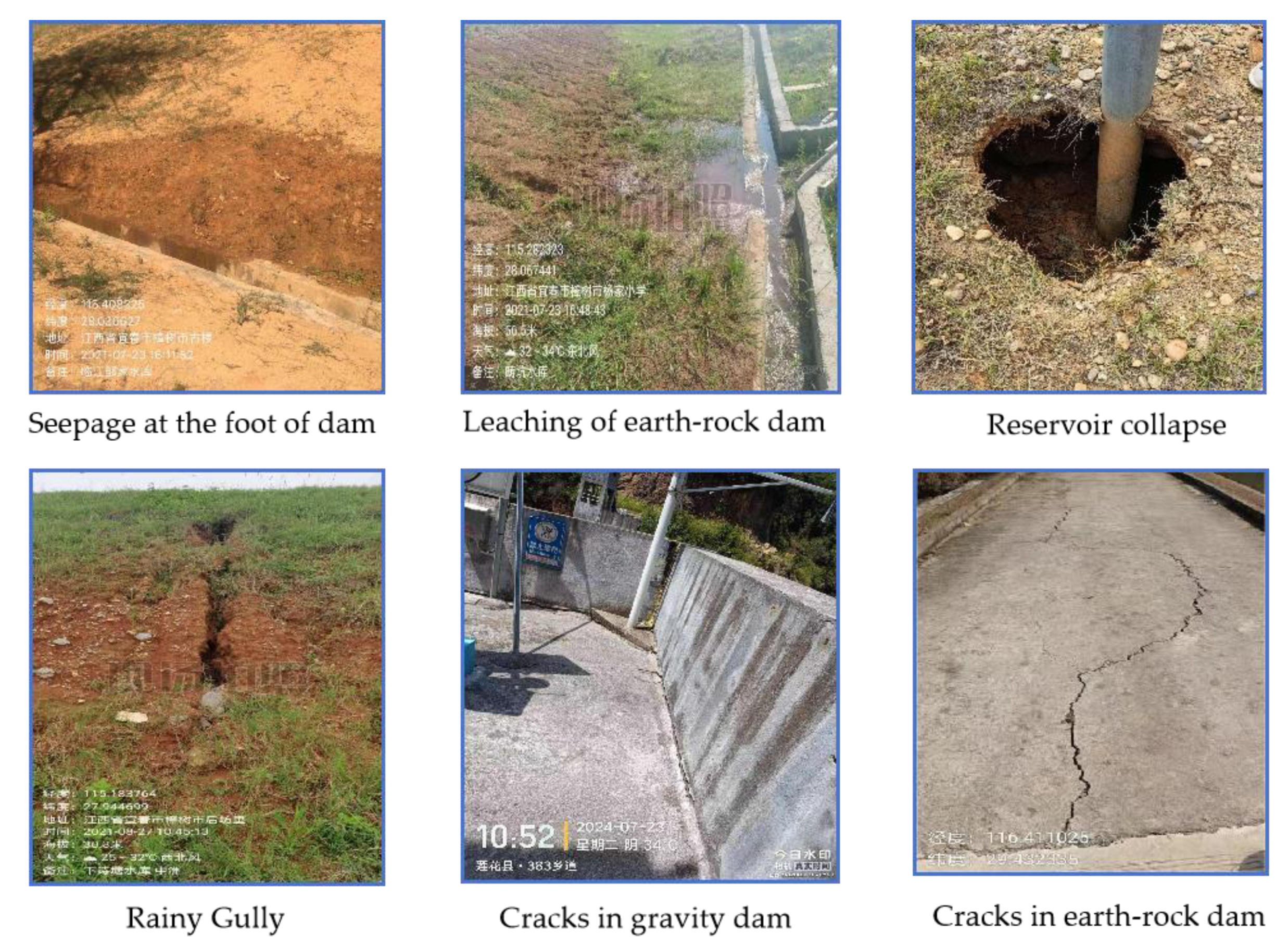
Climate Change and Extreme Weather Events: Global climate change has increased the frequency of extreme weather events such as heavy rainfall and floods, imposing greater water pressure and flood risks on small-scale reservoirs. This risk is particularly pronounced in mountainous and hilly regions, where extreme weather can destabilize the water body, increasing the risk of dam collapse or piping. Common hidden hazards in small-scale reservoir engineering include cracks, collapse, leaching, and seepage, as shown in Figure 1.

2.2. Image Data Sources for Hidden Hazard Detection

To accommodate the actual environment and hardware capabilities, sample images were captured using handheld devices and subsequently cropped to sizes suitable for processing. The CMOS image sensor is a critical factor determining the quality of the captured samples, with key performance indicators including the ability to restore received images, which depends on pixel array parameters. During image capture, the most direct parameters are sensor size, effective pixels, and shutter speed. The handheld device used is equipped with a 1/1.7-type Sony IMX600 image sensor with 40M square active pixels. Its CMOS image sensor achieves high-speed image capture through a column-parallel AD converter circuit and high sensitivity and low noise through a backside-illuminated pixel structure. It utilizes an R, G, and B color mosaic filter and incorporates lens shading correction, with dual sensors capable of synchronous operation. The IMX600 image sensor parameters are detailed in Table 1.

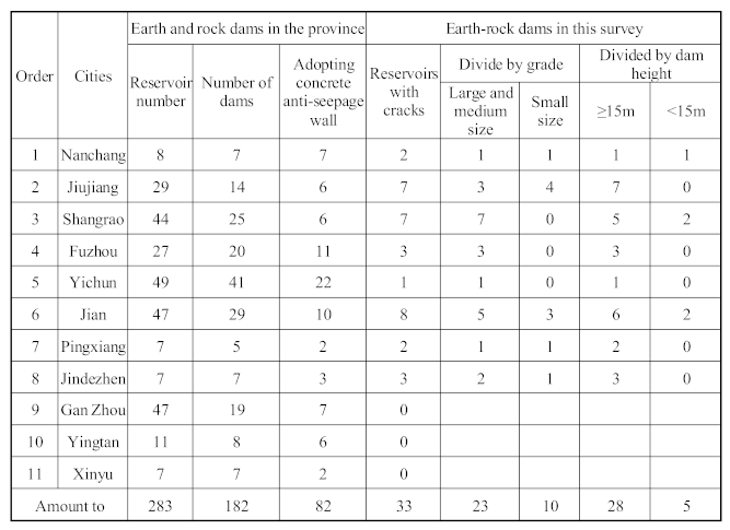
In order to further understand the hidden hazards, the Jiangxi Provincial Government conducted a survey on all small reservoirs in the province. According to the survey, among the 11 prefecture level cities (including directly administered counties) in the province, 33 earth and stone dams in 8 prefecture level cities including Nanchang, Jiujiang, Shangrao, Fuzhou, Yichun, Ji'an, Pingxiang, and Jingdezhen have cracks, as shown in Table 2.

According to the investigation, among the cracks in 33 dams, 79 cracks were investigated, as shown in Table 3.

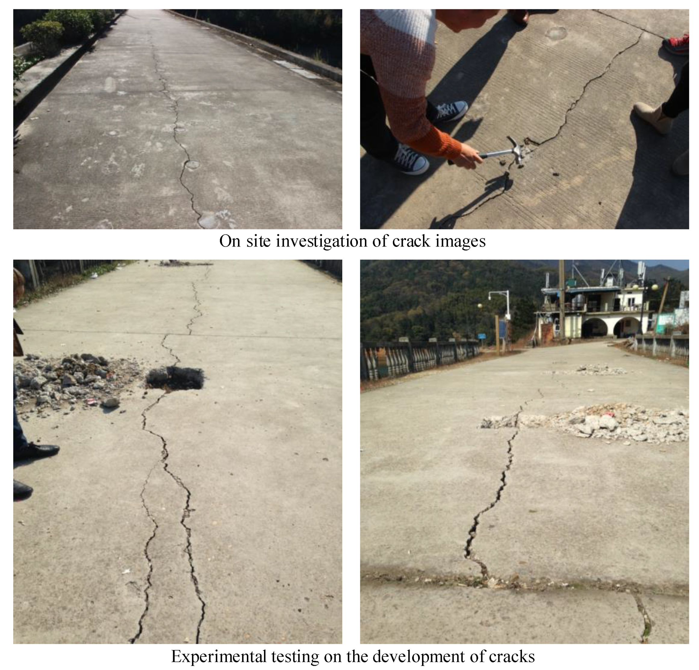
Cracks, as the most common hidden danger, have a significant impact on the safety of engineering in small reservoirs. Therefore, it is necessary to use image recognition combined with experimental data to study the development law of cracks. Figure 2 shows the testing of cracks.

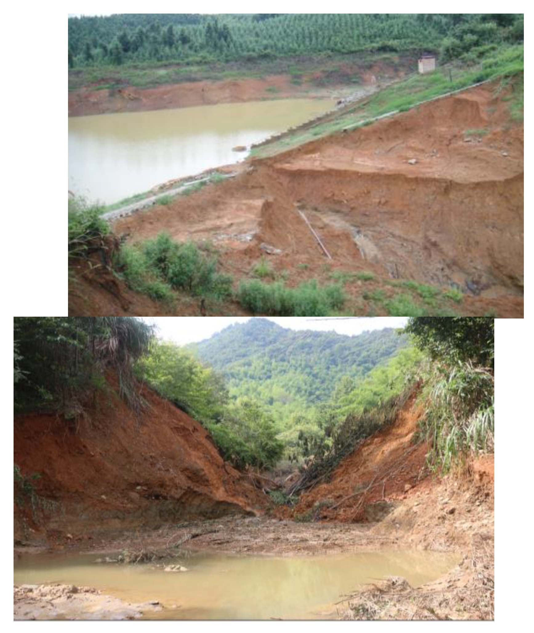
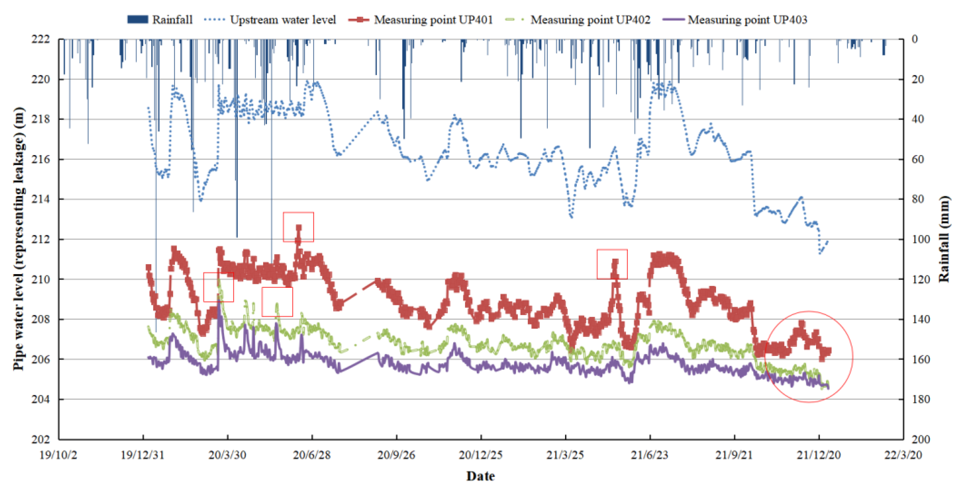
On the other hand, the leaching and seepage of small reservoirs caused by cracks or collapses are also worthy of the attention. The common path of reservoir dam failure is: flood → seepage damage → landslide → dam crest lowering → no manual rescue intervention → dam collapse, as shown in Figure 3. Time series correlation diagram of seepage under rainfall conditions is shown in Figure 4, according to the survey.

Under rainfall conditions, small reservoirs are particularly vulnerable to seepage, a critical safety concern that can lead to structural instability and potential failure. When rainwater infiltrates the embankments or foundations of a reservoir, it increases the pore water pressure within the soil, reducing the shear strength and potentially leading to internal erosion or piping. Seepage pathways can develop more easily during intense or prolonged rainfall, especially in areas with poor compaction or material defects. In small reservoirs, which often lack the sophisticated monitoring systems of larger dams, seepage can remain undetected until it reaches a critical stage. Signs of seepage include wet spots or boils on downstream slopes, increased water turbidity, or unexpected drops in reservoir water levels. In the context of heavy rainfall, these signs may intensify rapidly, as the hydraulic gradient between the reservoir water and the downstream area increases, forcing more water through any existing or newly formed cracks or weak zones.

Managing seepage under such conditions requires continuous monitoring and timely intervention. Utilizing advanced technologies such as UAVs and deep learning-based image analysis can help identify early signs of seepage, allowing for proactive maintenance and repairs. Additionally, employing geotechnical instruments, such as piezometers and seepage meters, can provide real-time data to assess the extent of seepage and guide decision-making to prevent structural failure and ensure the safety of the reservoir.

2.3. Dataset Construction

2.3.1. Data Collection

Data was collected from multiple sources, including UAV images, sensor data, and fixed camera data, ensuring coverage across sufficient time and spatial ranges, particularly in areas with high hazard occurrences. The target for image sampling was small-scale reservoir infrastructure in Jiangxi Province, focusing on cracks, seepage, and collapses of varying sizes and positions, with the smallest hazards (cracks) appearing as a single pixel in the image.

2.3.2. Data Preprocessing

Collected image data underwent data augmentation methods (e.g., rotation, translation, scaling) to expand the dataset and enhance model generalization. The original image samples were sized at 3648×2736 pixels, with 300 images containing hazards selected after screening. These images were first cropped to a size of 3648×1824 pixels for easier processing. Subsequently, the 3648×1824 images were horizontally cropped into 912×912 pixel images, and additional 912×912 pixel images were obtained through random cropping after rotating the original images. In total, 4800 images containing both hazard and non-hazard areas were produced. These 912×912 images were then uniformly resized to 256×256 pixels. After a second round of filtering, the images were categorized into two sets: one containing only background and the other containing hazards. The dataset construction involved selecting images with hazards, resulting in a final dataset of 4000 valid samples, which will undergo manual annotation in the next step.

2.3.3. Manual Annotation

Based on the image data, hazards such as cracks, collapses, and seepage were labeled, including their locations and severity. The open-source LabelImg tool was used for manual annotation, offering several annotation modes: classification, bounding box, segmentation, and brush-based segmentation. Given the significant differences among hazards, such as the fine and narrow cracks, a brush mode was used to color crack areas while leaving non-crack areas uncolored. Conversely, for larger areas like collapse zones, a bounding box mode was employed. The tool outputs labels in 32-bit RGB image format, with unannotated areas not displayed. Post-processing is needed to convert these labels for model input. Annotation is the most time-consuming step in dataset creation. Unlike common object detection tasks that require only drawing a rectangular bounding box around the object, semantic segmentation annotation for images requires marking the entire object area. This is particularly challenging for crack images, where cracks are thin and small, necessitating careful adjustment of brush width and frequent erasure of excess annotations. An example of the original crack image and the output label style from the LabelImg tool is shown in Figure 5. The annotated image is a 24-bit RGB three-channel image, with crack areas marked in red [255,0,0] and the background in transparent pixels [0,0,0]. The resulting 32-bit label image is not optimal for computer processing. Given that the pixel data in this study falls into two categories, the 32-bit label images will be converted to 8-bit images for easier data reading in subsequent processing.

The processed dataset was divided into training, validation, and test sets to ensure model training, validation, and testing on different data, enhancing model reliability and stability.

3. Deep Learning Based Semantic Segmentation Model for Hidden Hazards Images

3.1. Network Architecture for Hazard Segmentation

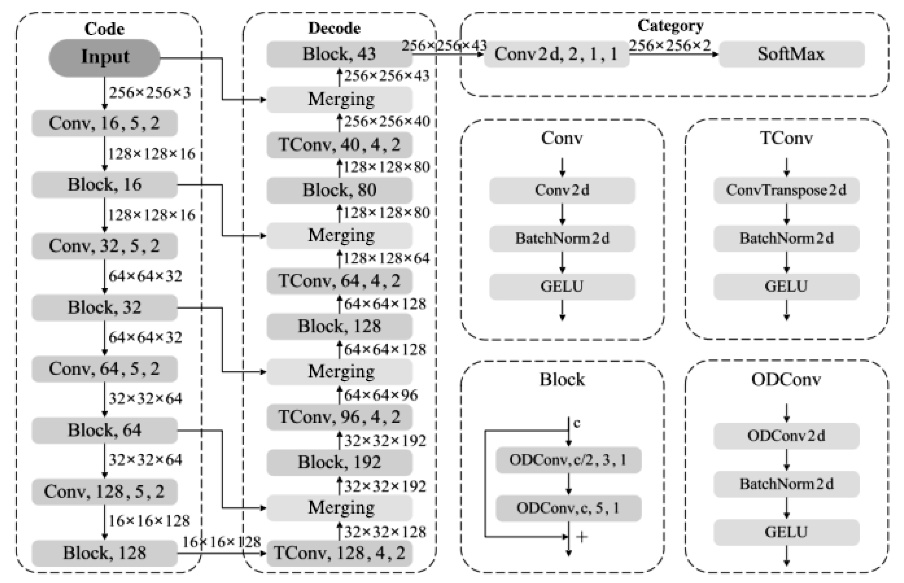
The proposed high-performance semantic segmentation method for detecting hazards in images of small-scale reservoirs is illustrated in Figure 6. The network comprises three main components: an encoder, a decoder, and a classifier. The overall structure consists of 12 encoding layers, 12 decoding layers, and 1 classification layer, making a total of 25 layers, which we have named HHSN-25 (Hidden Hazard Segmentation Network with 25 layers). The encoder structure is built from convolutional blocks (Conv) and residual blocks (Block). The Conv block comprises a 2D convolution (Conv2d), Batch Normalization (BN), and a GELU activation function, while the Block contains two ODConv units. Each ODConv unit is made up of an omni-dimensional dynamic convolution (ODConv2d), BN, and GELU activation. The primary role of the encoder is to reduce feature dimensions and increase network depth, thereby expanding the receptive field to capture more hazard-related features.

The decoder consists of transposed convolutional blocks (TConv) and Blocks. The TConv block includes a 2D transposed convolution (ConvTranspose2d), BN, and GELU activation function. The main purpose of the decoder is to recover the original image dimensions while further extracting hazard features, merging multi-dimensional features from various stages of the encoder for pixel-level classification. The classification layer is a 2D convolutional layer that transforms the dimensions along the channel direction to match the number of classes, with a SoftMax function used to predict the probability of each pixel belonging to a specific class. In the HHSN-25 structure, parameters for each sub-module are specified as module name, output channels, kernel size, stride.

3.1.1. Feature Dimension Transformation in the Hazard Segmentation Network

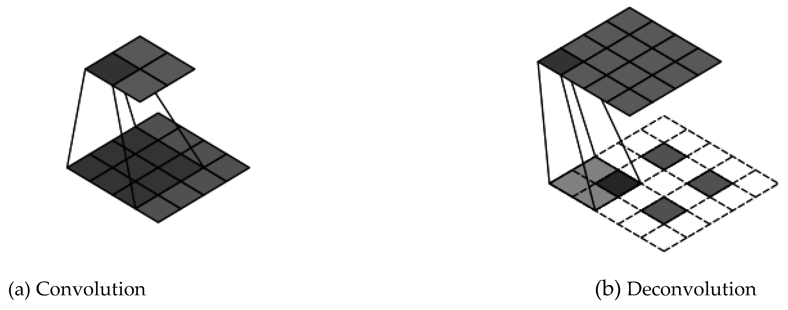
The transformation of feature dimensions in a typical deep learning network involves two aspects: changes in feature map size and feature map count. Regarding feature map size, convolution and transposed convolution operations are primarily responsible for altering dimensions. The convolution and transposed convolution processes for 2D images are shown in Figure 7.

Figure 7(a) demonstrates the process where a feature map of size 4×4 is convolved with a kernel size of 3, stride of 1, and no padding, resulting in a 2×2 feature map. Here, the stride represents the number of pixels the kernel moves at each step, and padding refers to adding blank pixels around the edges to accommodate the desired size. Figure 7(b) illustrates the reverse, where a 2×2 feature map is transformed via transposed convolution with a kernel size of 2, stride of 1, and padding of 1 to produce a 4×4 feature map. The input-output relationship for convolution and transposed convolution is given by specific equations:

o_{c o n v} = \frac{i - k + 2 p}{s} + 1

(1)

o_{t c o n v} = s (i - 1) - 2 p + k + [\frac{o + 2 p - k}{s}]

(2)

where o_conv and o_tconv represent the output size, and i is the input size, k is the kernel size, s is the stride, and p is the padding. The second aspect of dimension transformation concerns the change in the number of channels. Increasing the number of channels while downsampling along spatial dimensions is crucial for network performance, as it enhances the diversity of high-level features. In HHSN-25, the encoder increases the number of channels as the feature map dimensions decrease, while the decoder decreases the number of channels as the feature map dimensions are restored. This design adheres to the feature pyramid principle, optimizing memory use.

3.1.2. Basic Feature Extraction Structure of the Hazard Segmentation Network

Increasing the network depth helps expand the receptive field and extract higher-level features. Since the introduction of ResNet, skip connections have become the dominant structure in deep learning, such as in ConvNeXt, which improves network performance by using skip connections and increasing kernel size. The basic feature extraction structure (Block) in HHSN-25 adopts the skip connection concept from ResNet, integrating omni-dimensional dynamic convolution and experimentally verified optimal kernel sizes.

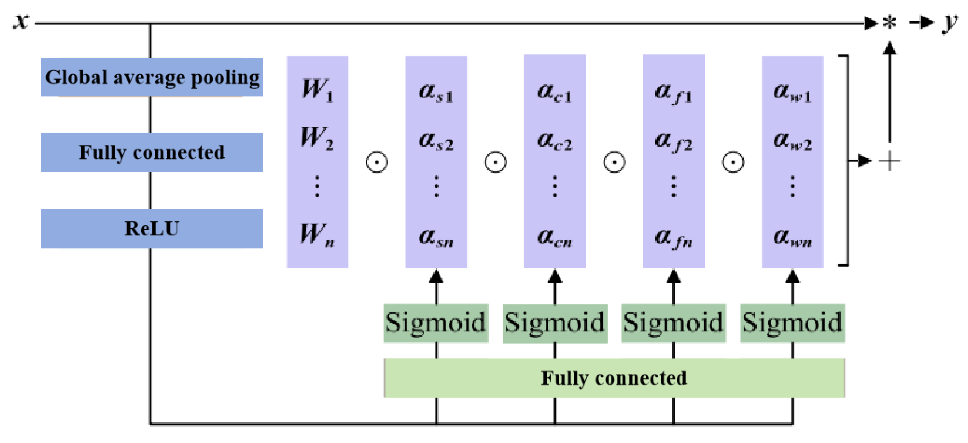
The ResNet structure consists of two convolutions with a kernel size of 3. The first convolution is followed by BN and a ReLU activation function; the second is followed by BN, with the skip connection then linked to a ReLU activation function, keeping the feature map size unchanged throughout. In ConvNeXt, the input first passes through a depthwise convolution with a kernel size of 7 and Layer Normalization (LN), followed by a pointwise convolution with a kernel size of 1 to increase the channel count fourfold, activated by GELU. A final pointwise convolution restores the channel count before the skip connection. The Block in our study applies two omni-dimensional dynamic convolutions with kernel sizes of 3 and 5, followed by skip connections, each convolution operation incorporating BN and GELU activation. The omni-dimensional dynamic convolution introduces a multi-dimensional attention mechanism, employing a parallel strategy to learn different attentions across four dimensions in kernel space. The basic structure of the omni-dimensional dynamic convolution used in this study is depicted in Figure 8.

This convolution utilizes a SE-style attention module with multiple heads to compute various types of attention. For input data, global average pooling, fully connected layers, and ReLU activation functions reduce it to a one-dimensional feature vector, which is then processed by four fully connected heads to produce different attention values. The four attention dimensions focus on position, channel, filter, and kernel, capturing richer contextual information. The omni-dimensional dynamic convolution utilizes a new multi-dimensional attention mechanism, calculating four types of attention across all four dimensions in parallel within the kernel space:

y = (α_{w 1} ⨀ α_{f 1} ⨀ α_{c 1} ⨀ α_{s 1} ⨀ W_{1} + \dots α_{w n} ⨀ α_{f n} ⨀ α_{c n} ⨀ α_{s n} ⨀ W_{n}) * x

(3)

where, α_w1 represents the attention scalar of the convolutional kernel, α_s1, α_c1 and α_f1 represents the three newly introduced attention points, which are calculated along the spatial dimension, input channel dimension, and output channel dimension of the convolutional kernel. ⊙represents the multiplication operation along different dimensions of the kernel space.

3.2. Loss Function and Improvements for the Hazard Segmentation Network

Among various deep learning-based image semantic segmentation methods, Cross Entropy (CE) is the most commonly used function for loss calculation, analyzing each pixel separately and comparing predicted values for each pixel class with the ground truth. This approach assigns the same weight to every pixel during loss calculation, which may not be ideal for segmentation tasks involving imbalanced pixel distributions. The CE loss function expression is as follows:

C E_{L o s s} = - \sum_{c = 1}^{M} y_{c} \log (p_{c})

(4)

where M represents the number of categories, and y_c is a one hot vector with element values of only 0 and 1, and p_c represents the probability that the predicted sample belongs to class c. When there are only two categories, the Binary Cross Entropy (BCE) loss function can be expressed as:

B C E_{L o s s} = - \sum_{c = 1}^{N} [y_{c} \log (p_{c}) + (1 - y_{c}) \log (1 - p_{c})]

(5)

where, p_c represents model input and y_c represents real labels. The Binary Cross Entropy with Logits (BCEL) loss function is a loss function that combines a Sigmoid layer and BCE loss into a single category. Shrivastava et al. [20] proposed an algorithm for online hard example mining (Ohem) to address the issue of imbalanced positive and negative samples. The OhemCE loss function first calculates the cross entropy loss, then selects difficult samples based on the loss, and finally applies higher weights to them in subsequent training. The Intersection over Union (IoU) loss function is commonly used in object detection, which reflects the ratio of the intersection and union of annotated and predicted values. It is also commonly used for loss calculation in image semantic segmentation. The loss expression of IoU is as follows:

I o U_{L o s s} = 1 - \frac{A \cap B}{A \cup B}

(6)

Focal Loss (FL) is commonly used to deal with class imbalance. It determines the weight of class related losses based on the difficulty of distinguishing class samples, that is, applying smaller weights to easily distinguishable samples and larger weights to difficult to distinguish samples. The FL expression is as follows:

F o c a l_{L o s s} = - \sum_{c = 1}^{M} {(1 - p_{c})}^{γ} y_{c} \log p_{c}

(7)

FL adds a weighting coefficient

{(1 - p_{c})}^{γ}

before the standard CE function. The Dice loss function is named after the Dice coefficient, which is a metric used to evaluate the similarity between two samples and can effectively represent their similarity. The Dice loss function is expressed as follows:

D i c e_{L o s s} = 1 - 2 \times \frac{|A \cap B|}{|A| + |B|}

(8)

where, A represents the pixel labels of the actual segmented image, and B represents the pixel class prediction of the segmented image by the model. Considering the disproportionate nature of hazard pixels and background pixels in crack images, this chapter uses FL combined with Dice coefficient for loss calculation, which is expressed as follows:

L o s s = 1 - \sum_{c = 1}^{M} {(1 - p_{c})}^{γ} y_{c} \log p_{c} - \frac{2 I + ε}{U + ε}

(9)

where, I represents the intersection of correctly identified pixels, U represents the union of prediction and label, and ε is the smoothing coefficient.

4. Results

4.1. Experimental Environment and Evaluation Indicators

All models in this topic are trained and verified on the Windows11 operating system. The hardware configuration is AMD Ryzen 7 series 5800H processor, equipped with 16GB running memory, and the display card is NVIDIA RTX3060 mobile terminal platform equipped with 6GB display memory. The deep learning framework is the pytorch, CUDA 11.6 environment. Furthermore, due to memory limitations, the number of multiple threads and the size of batch processing were set to 4, and different sets of hyperparameters were analyzed during training to select the best validation model configuration. Each dataset was split into 80% (3200 images) for training, 10% (400 images) for validation, and 10% (400 images) for testing. All image input sizes used in the experiment were set to 256×256.

The easiest way to do this is to calculate how many pixels are being correctly segmented, but this is not enough. The essence of crack image segmentation is to evaluate each pixel using a classifier, so the result of a pixel consists of two kinds: correct and wrong. Since the hidden danger data set is a data set with unbalanced category pixels, if the average accuracy is simply used as the evaluation index, the accuracy of the hidden danger pixels will be covered by the accuracy of the background pixels, and the results will not be well observed. In this experiment, the average intersection ratio (mean Intersection over Union, mIoU) was used as the main performance evaluation index, and the precision rate (P), recall rate (R), F1, Accuracy, Mean Pixel Accuracy (mPA) score were also considered [15]. These indicators are mainly obtained from the confusion matrix, which can be expressed by the true case TP, true negative case TN, false positive case FP, and false negative case FN.

4.2. Comparison of the Experimental Results

4.2.1. Basic Feature Extraction Structure Block

For small hidden danger pixels (such as cracks), theoretically only a small window is needed to identify their features, and the existing hidden danger image segmentation methods are mostly improved based on the current mainstream methods, among which a large number of methods to expand the feeling field may be too radical. Convolutional neural network mainly by expanding the convolution kernel and deepening network depth expand feeling field, in order to study the appropriate structure, the basic feature extraction structure Block using the performance of the kernel experiment, then studied the introduction of the full dimensional dynamic convolution model, will also proposed the Block structure compared with the performance of several other mainstream network module. The effect of different convolution kernel sizes in Block on the network is shown in Figure 9, where k values in turn represent the convolution kernel sizes of the two convolutional layers in Block. From the experiment, we can first see that the effect of using full-dimensional dynamic convolution(ODConv) is better than that of ordinary convolution. Second, the effect is better when the k values are taken successively at 3 and 5. In addition, the actual mIoU gap in the three sets of experiments using full-dimensional dynamic convolution is less obvious than the ordinary convolution, which further proves that the attention of different dimensions improves the network performance.

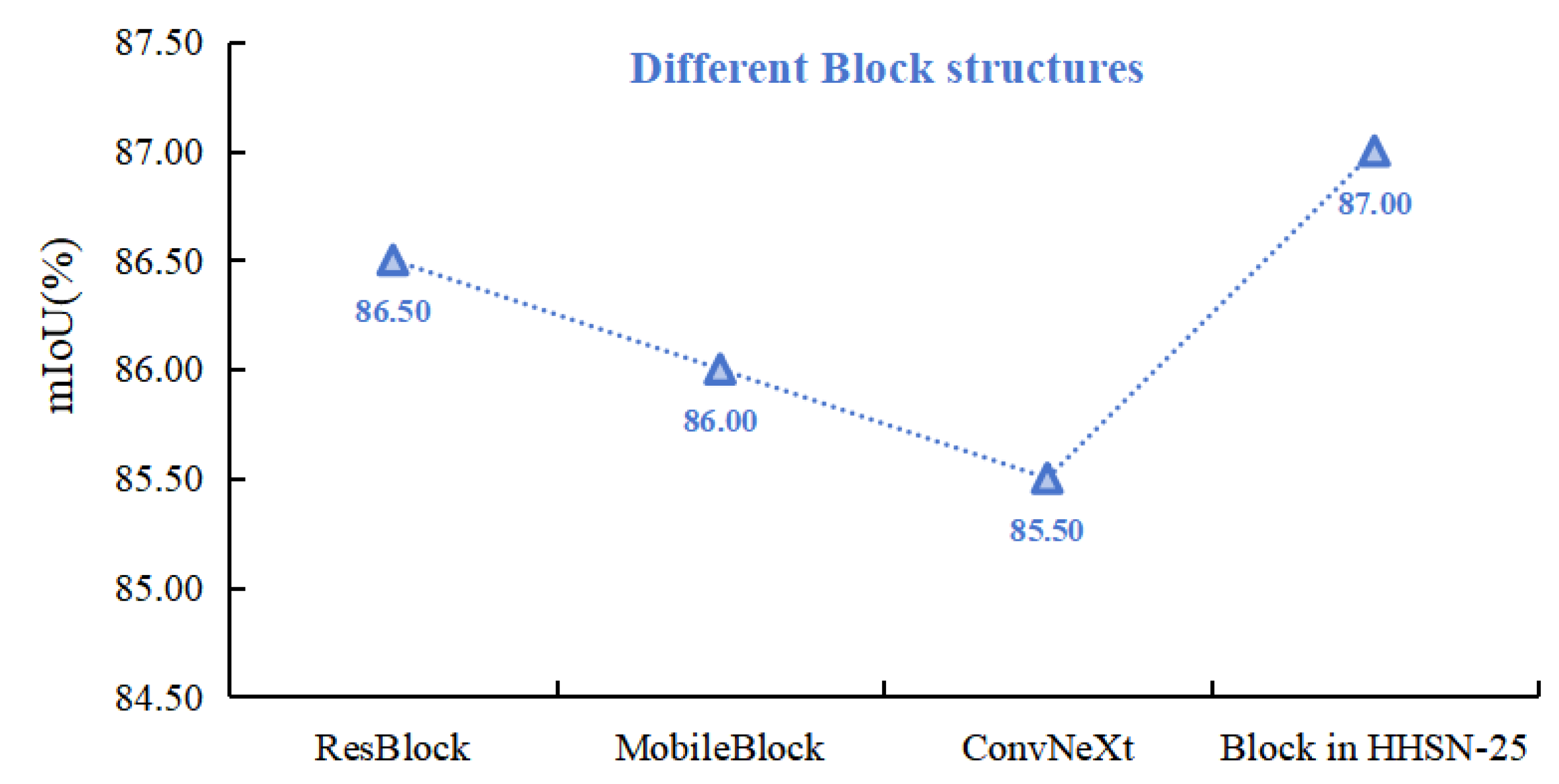
The performance of ResNet, MobileNetV3 and ConvNet feature extracted structures ResBlock, MobileBlock, ConvNeXt and Block in HHSN-25 is shown in Figure 10. It can be seen that ConvNeXt structure has the lowest performance in the crack image segmentation task, while the performance of Block phase is significantly improved compared with other structures.

4.2.2. Comparison of Changes in Different Network Widths in Decoding Structures

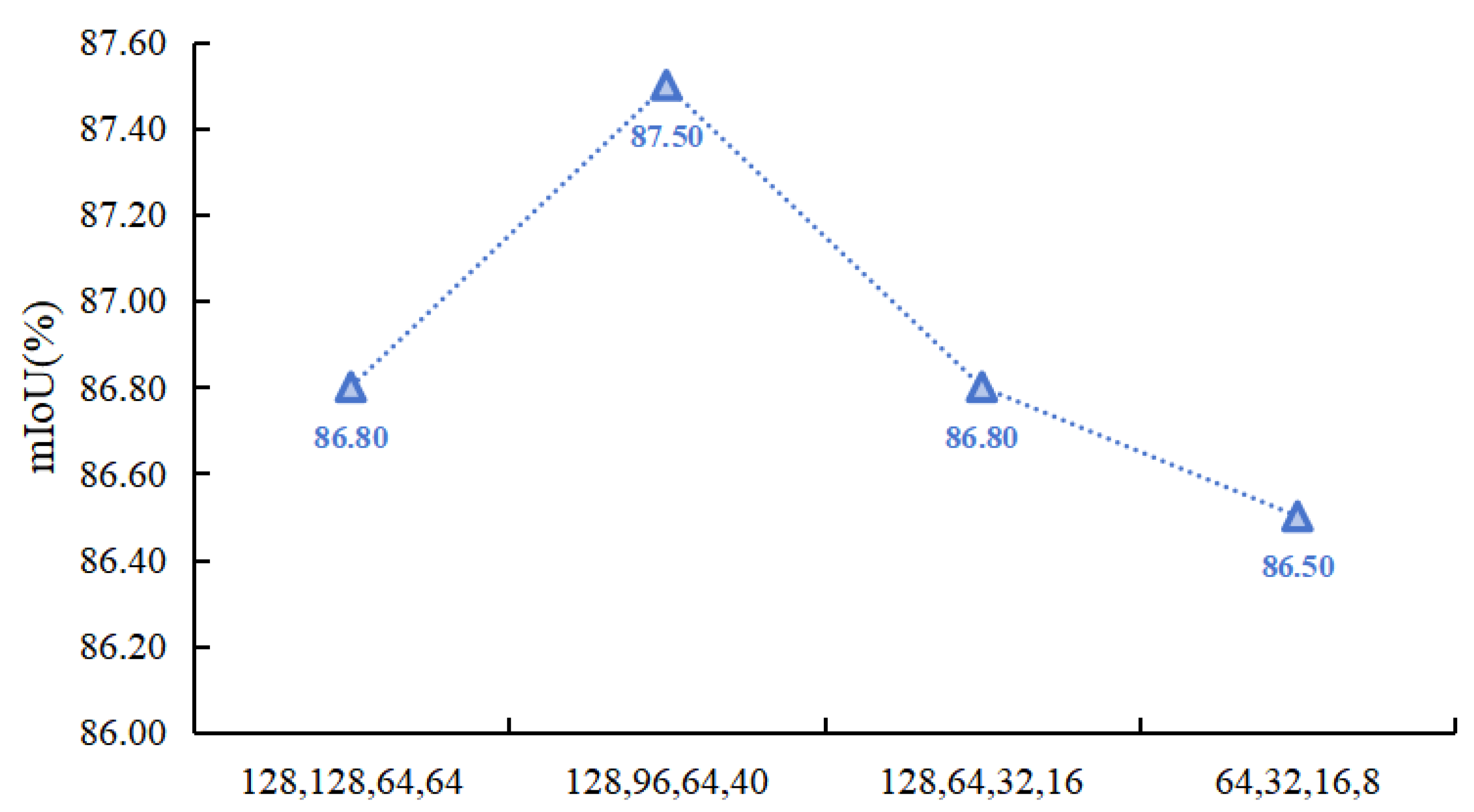
The pyramid structure is a pattern of network width that has been proven to be suitable in convolutional neural networks through research. In actual network construction, feature maps are usually upsampled and downsampled for dimensionality reduction, and the number of channels decreases and doubles accordingly. In HHSN-25, if the number of feature image channels recovered during the decoding process corresponds to the encoding structure, some hidden features may be lost during this process, but the additional feature channels will increase the computational resource consumption of the network. Therefore, it is necessary to study the variation law of features in the channel dimension during the decoding stage. As shown in Figure 11, the comparison of the changes in four different network widths is presented, which is reflected by the number of feature channels during each dimensionality increase. The horizontal axis represents the number of feature channels output after four dimensionality increase operations during the decoding process. The experimental results showed that the network performance was optimal when the number of channels was 128, 96, 64, and 40, respectively. In this feature fusion strategy, the number of channels was doubled before and after each dimensionality upgrade, while the results with the number of channels 64, 32, 16, and 8 were significantly lower than the other three results. The reason for this is that excessive reduction in the number of channels during dimensionality upgrade resulted in fewer hidden feature information being included in the fewer channels.

4.2.3. The Influence of Different Loss Functions on the Experimental Results

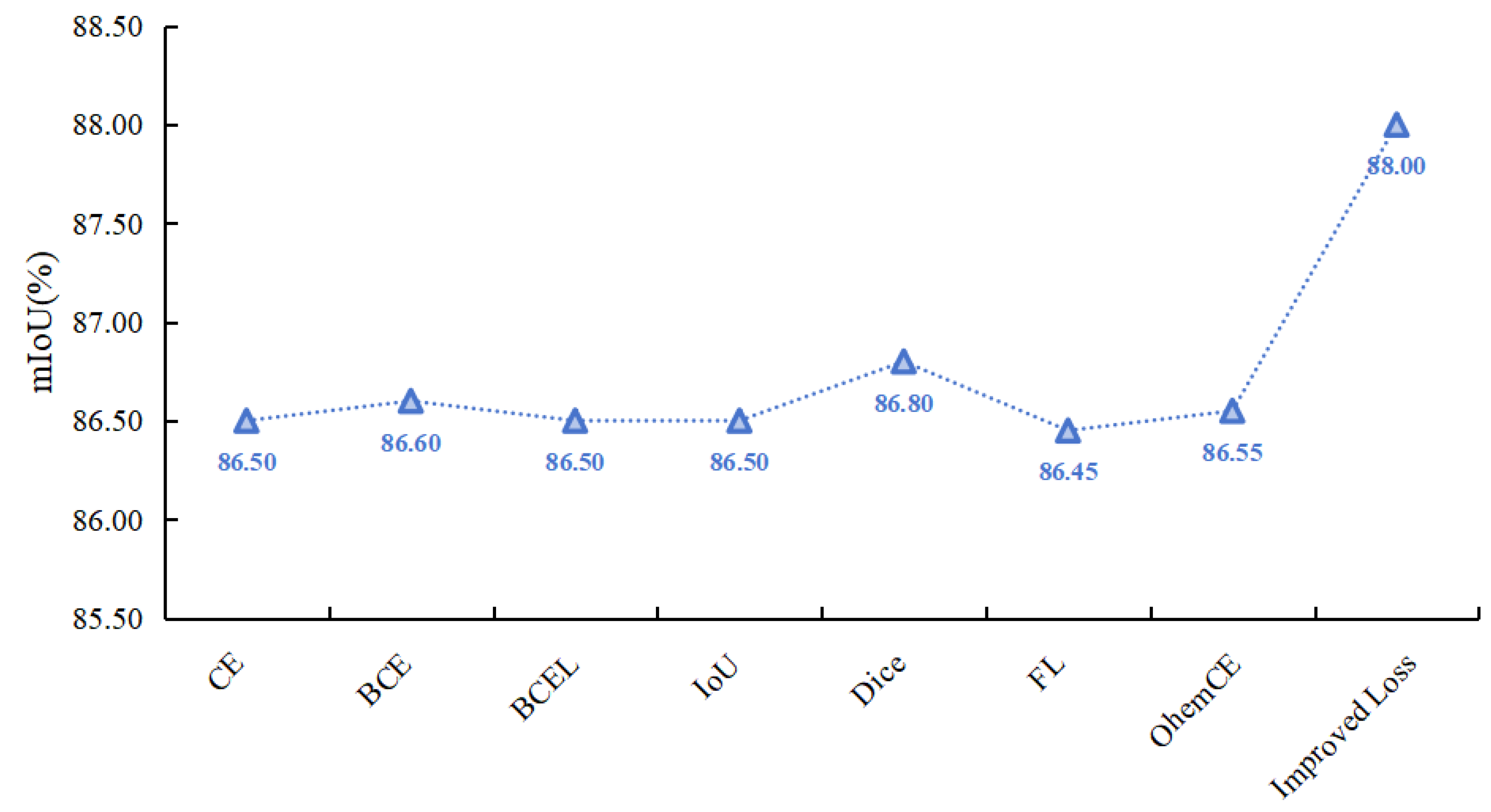
The performance comparison of HHSN-25 network using different loss functions is shown in Figure 12. It can be seen that due to the improved loss function focusing on the similarity of different samples, the attention to different samples is different. Using the improved loss function in this project for loss calculation yields the best results, significantly higher than the results of other loss functions.

4.2.4. The Performance Comparison of Different Segmentation Methods

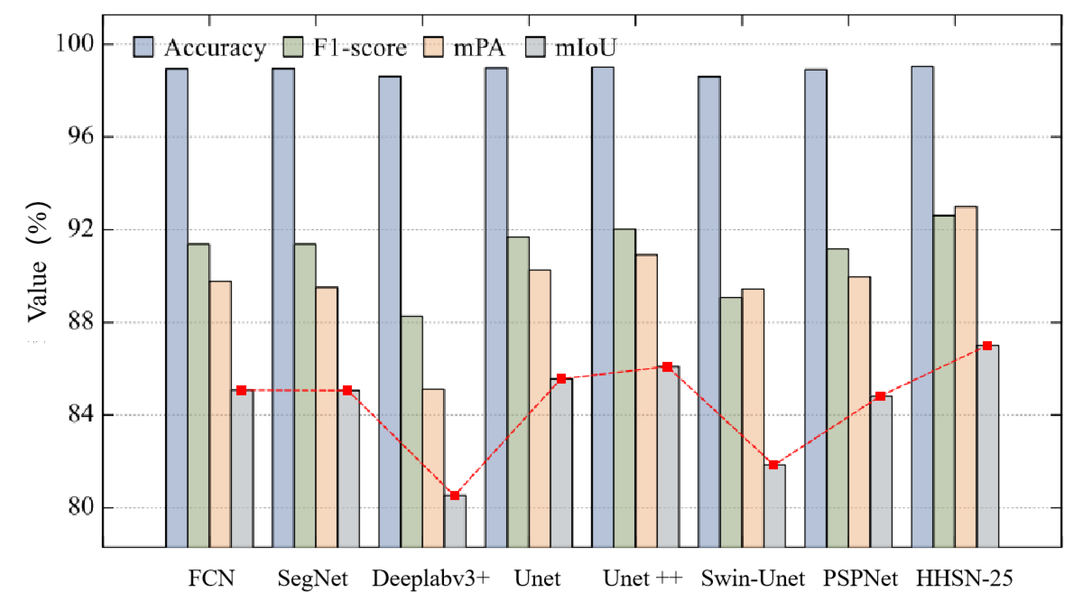
To verify the effectiveness of the HHSN-25 network proposed in this chapter, its experimental results were compared with those of other segmentation methods, as shown in Figure 13. It can be seen that in the graphical data of the main evaluation indicator mIoU, HHSN-25 is significantly higher than other methods, reaching 87.00%, FCN is 85.00%, SegNet is 85.00%, Deeplabv3+is 80.50%, Unet is 85.50%, Unet++is 85.55%, Swin-Unet is 82.00%, and PSPNet is 84.50%. In addition, among the other commonly used evaluation indicators in Figure 13, HHSN-25 outperforms other methods.

Meanwhile, from Figure 13, it can be seen that there is almost no difference in the accuracy index of these methods. This is because the number of hidden pixels is much less than that of background pixels. When calculating them together, the large base of background pixels will weaken the expression ability of this index for hidden pixels. This also explains why Accuracy was not used as the main evaluation index in this project. When calculating the F1 score and mPA index, the indicators of hidden and background pixels are first calculated separately, and then the average value is taken. Therefore, it can better reflect the overall classification effect of background pixels and hidden pixels, and is also within the reference range for evaluating the performance of the network.

4.2.5. Other Experimental Results

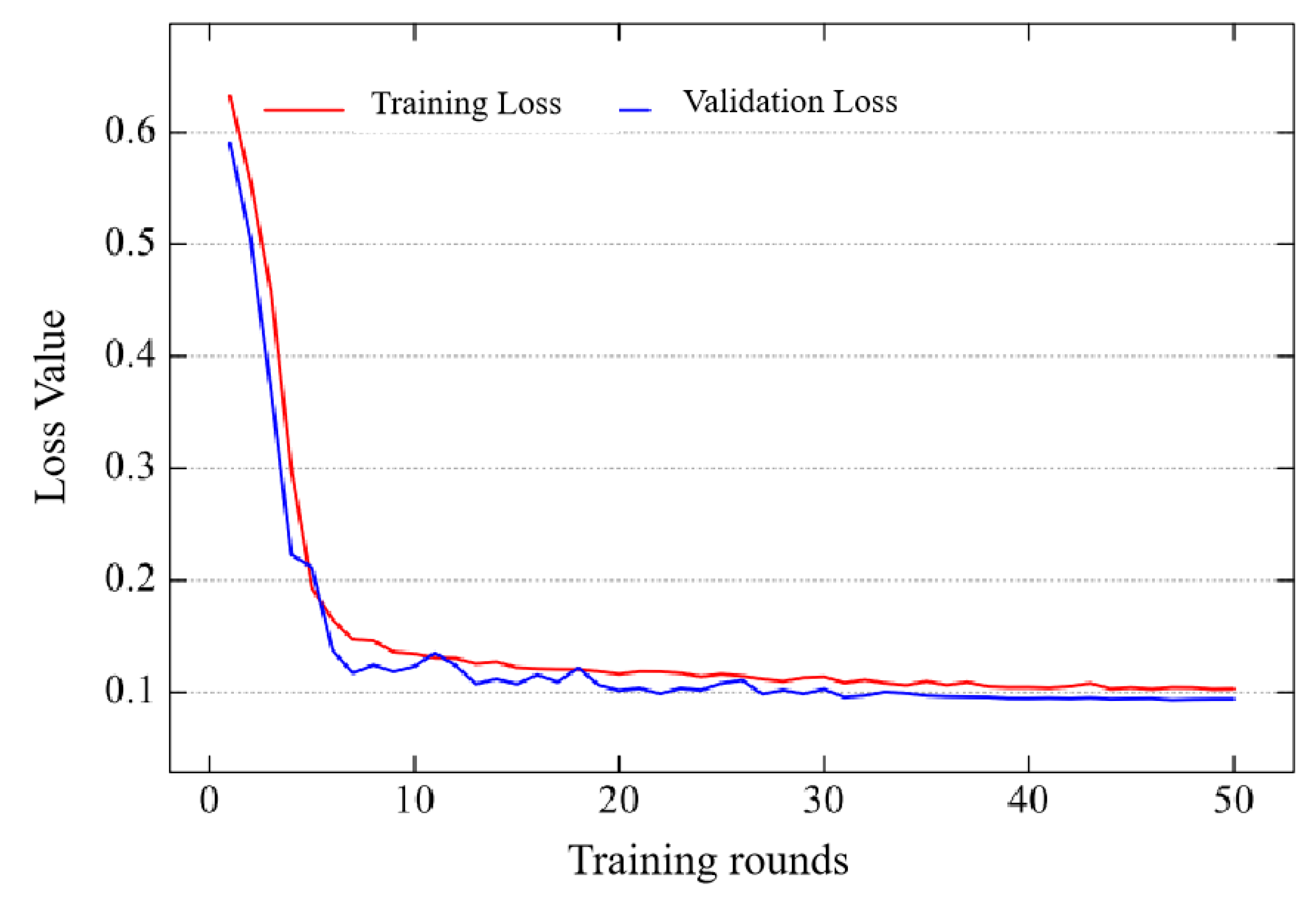
The loss function can be used to better describe the difference between the predicted value and the true value of the model, and the smaller the loss value, the better the performance of the model. During the training process of the model, the loss value decreases with the increase of training rounds until convergence, at which point the model usually achieves good results. The convergence of the loss function during the experiment is affected by factors such as data, network, and environment. As shown in Figure 14, the loss value of HHSN-25 during training shows the trend of change with the number of training rounds. It can be seen that the loss value has hardly changed by the time it reaches 50 rounds of training, which also explains the reason for choosing 50 rounds of training in this experiment. If the number of training rounds is too small, the model may not converge, resulting in poor performance and cannot be used as a basis for comparing the final experimental results. If there are too many training rounds, on the one hand, it will consume more time, and on the other hand, the network performance improvement will not be significant, and it may cause overfitting.

In addition, due to the different loss functions of each method during training, even if their values are scaled to the same range, they cannot be used as a basis for comparison due to the different calculation methods. Figure 14 is only used as a training network, and the main means of measuring the performance of these methods is still to compare the quality of mIoU values, reflecting the final segmentation effect.

5. Discussion and Application

Based on the HDSN-19 image semantic segmentation method framework, extract hidden hazard image features and quantify them:

Crack length and width

Find the boundary of the target object in the segmentation result (edge detection); Use the bounding box or fitting ellipse to fit the target object and obtain its length and width.

Use the height and width of the bounding box to represent the length and width of the target object.

Leaching area, leakage area, and collapse area

Calculate the number of pixels within the target object area (the area of the segmentation region).

Convert pixel area to actual area (given the spatial resolution of the image, i.e. the actual physical size corresponding to each pixel).

Area=number of pixels in the segmented area multiplied by the actual area per pixel.

5.1. Integration of Hidden Hazard Feature Extraction Algorithm

The trained image hidden feature extraction algorithm has been integrated into edge devices and carried out demonstration applications. During actual operation, the collected images need to be clear enough to identify small structural changes such as cracks or leaks. The camera equipment needs to be able to capture the target area video clearly within a certain distance, with a distance of less than 50 meters. As such, a high-definition (higher than 1080p resolution) camera has been used to ensure rich details in the image. This ensures that the data collected under different environmental conditions is of sufficient quality, so that the model can accurately detect and identify engineering hazards.

Through the edge computing architecture, this algorithm realizes real-time monitoring and analysis, and reduces the total time from data acquisition to hidden danger detection and alarm from the original average of 5 minutes to 40 seconds (reduced by about 86%). The high-performance embedded processor NVIDIA Jetson AGX Xavier and software configuration (TensorFlow, PyTorch) are specially designed for edge computing, so that it has efficient processing capacity and low energy consumption, and is suitable for real-time data processing and analysis. In addition, the edge computing architecture enables data processing to be completed locally, reducing dependence on the cloud, improving response speed and privacy protection. Comparing the adaptive detection model developed in this project with the mainstream method "Edge AI and Machine Learning", Table 4 can be obtained. The results indicate that the differences between the two are mainly reflected in the data processing and resource requirements during model training and inference computation. The deep learning method of the detection model developed in this project does not rely on manually annotated data, thus reducing the need for annotated data when training on edge devices. After the model training is completed and integrated, the inference calculation process is relatively fast and the computation time is relatively short. In addition, the multimodal data fusion and adaptive deep learning model have improved the anti-interference ability of the research and development model in complex environments, enabling it to dynamically adjust and adapt to sudden changes in the environment, and play an advantage in scenarios where data annotation is difficult. The training process of Edge AI and Machine Learning is usually completed in the cloud. When reasoning on edge devices, due to the use of pre trained models and optimization techniques, the performance in dealing with sudden changes in environments (such as night, rain, and fog) is weak and the adaptability is poor.

5.2. Algorithm Promotion and Practical Application

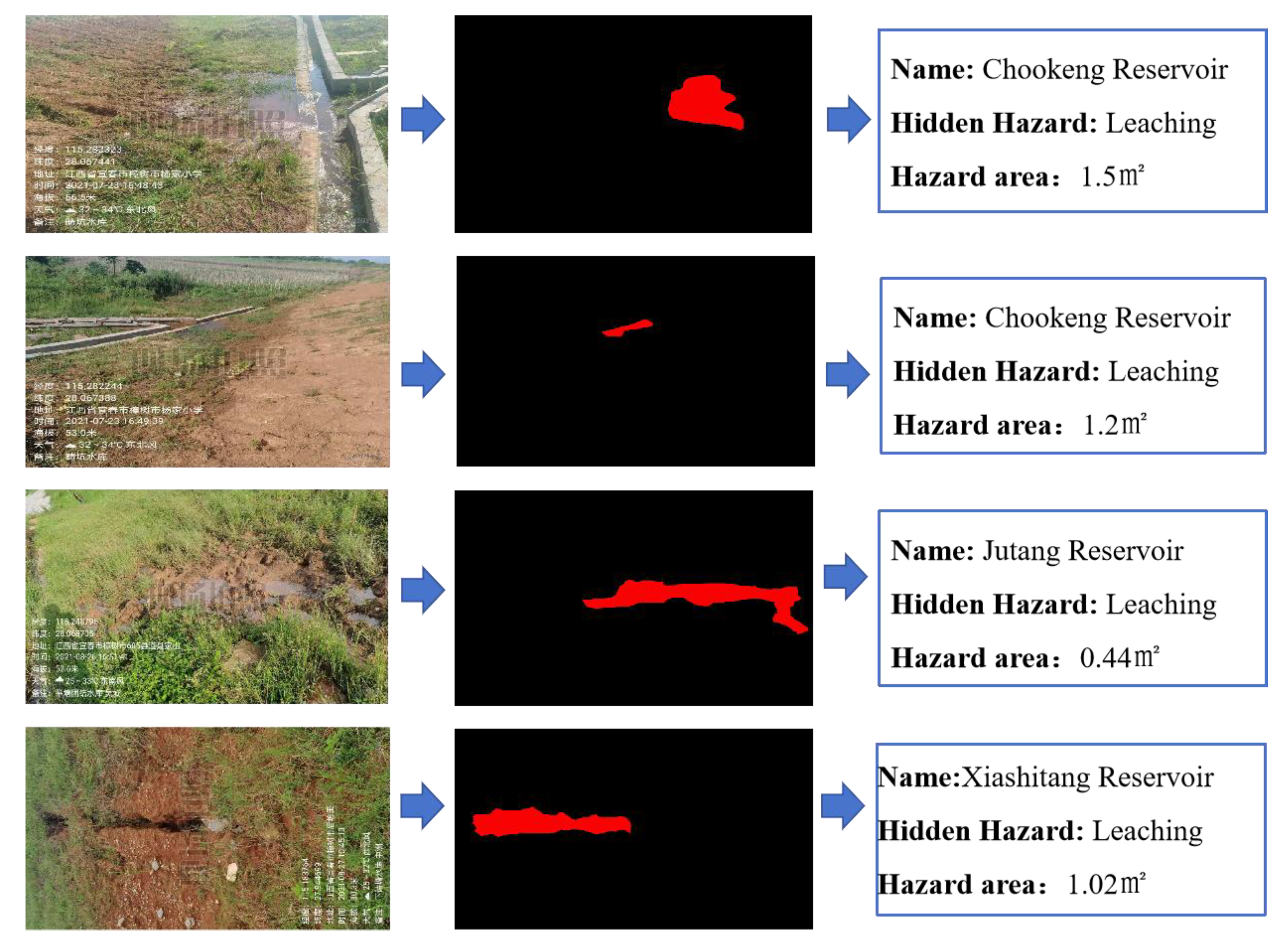
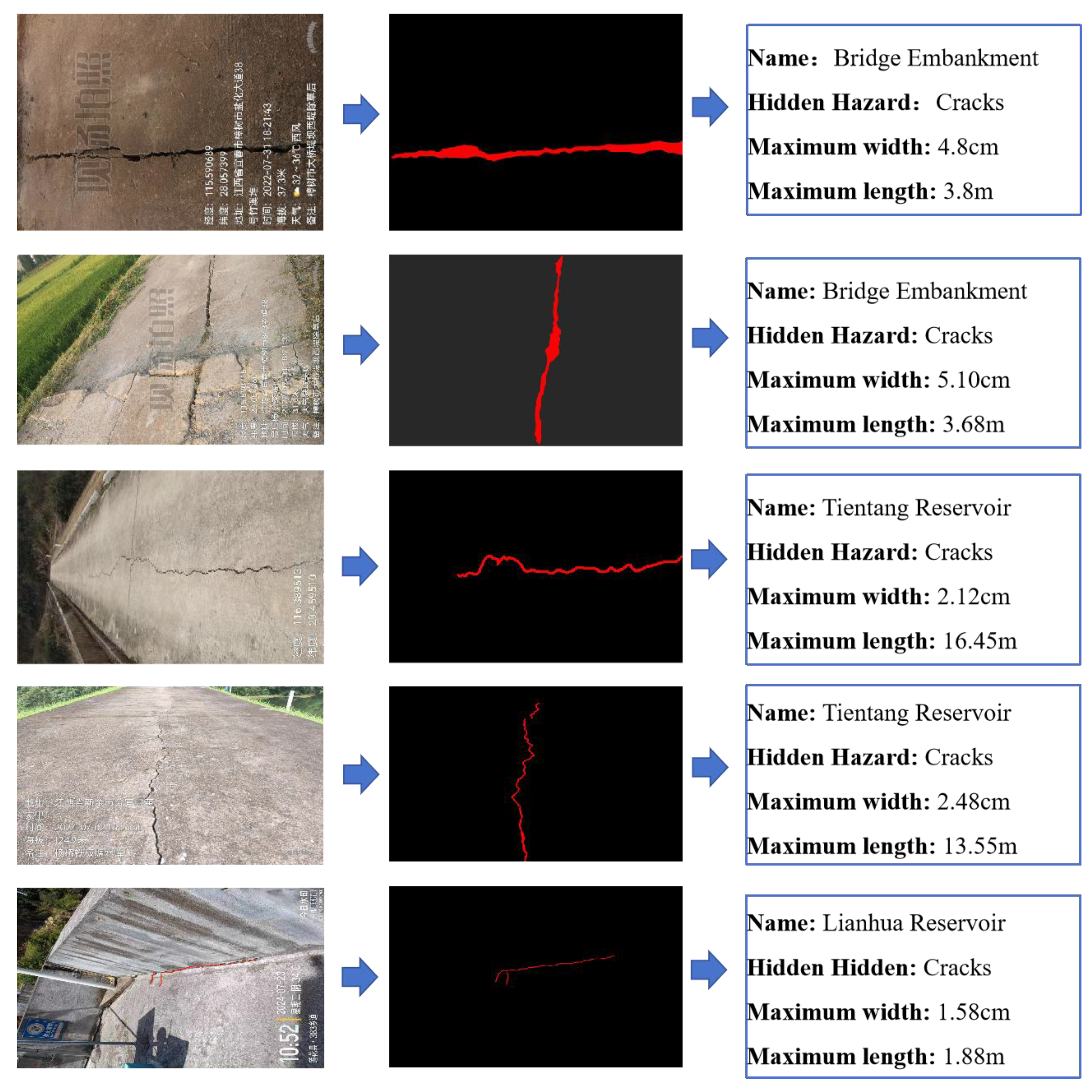
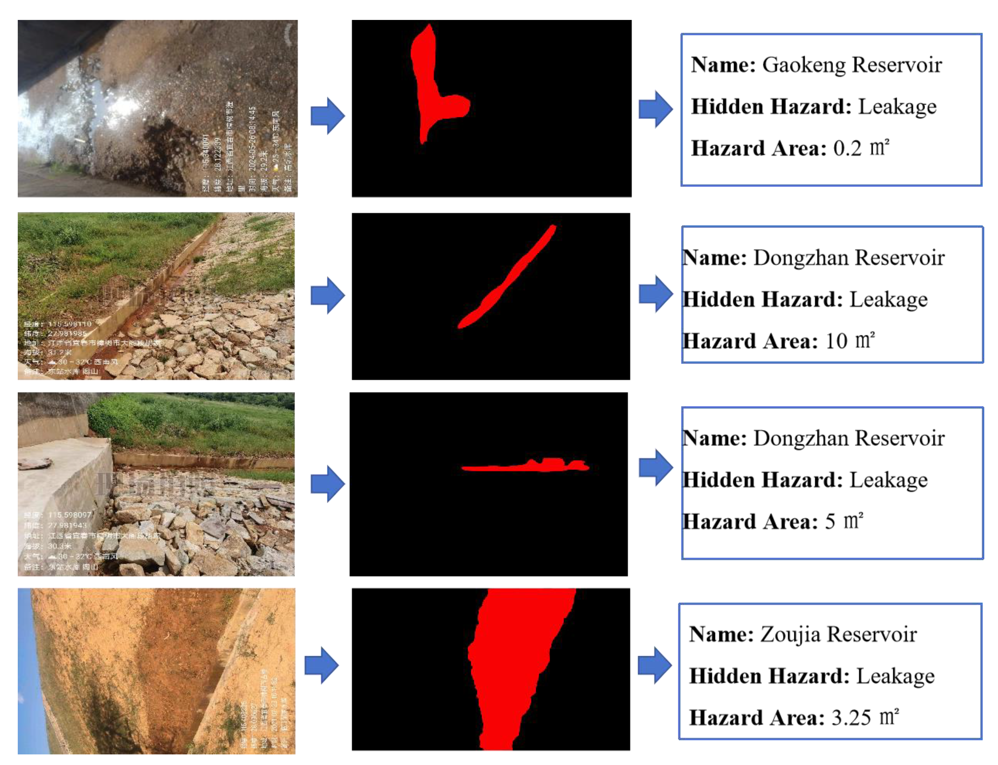
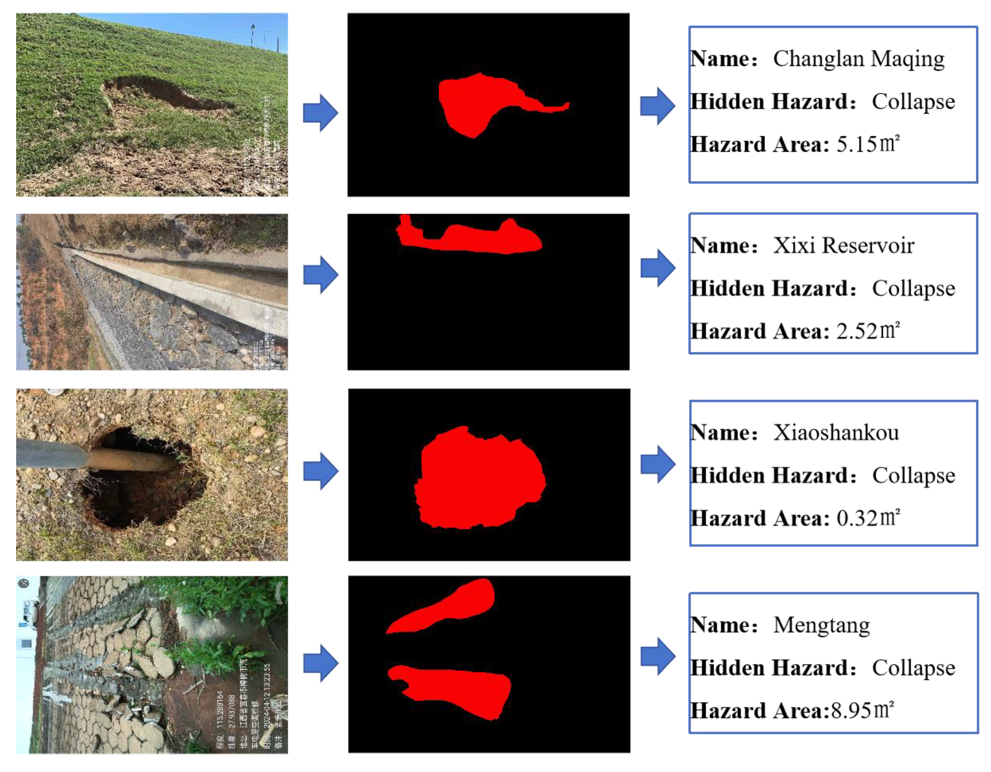
To sum up, the project not only significantly improves the accuracy and recall rate of hidden danger detection of small reservoir projects, but also greatly shortens the detection and response time and significantly improves the safety and operation efficiency of reservoirs by integrating edge computing hardware and software configuration, optimizing response speed and adopting advanced multi-source data fusion and image segmentation adaptive models. At the same time, the image hidden danger feature extraction algorithm has been widely applied in multiple typical reservoirs, including 25 small reservoirs in Jiangxi Province, including Chookeng Reservoir, Jutang Tuanjie Reservoir, Xiashitang Reservoir, Gaokeng Reservoir, Dongzhan Reservoir, Linjiang Zoujia Reservoir, Zhangshu City Daqiao Dam, Yangqiao Tientang Reservoir, Lianhua County Reservoir, Changlan Maqing Dam, Xixi Reservoir, Xiaoshankou Reservoir, Mengtang Reservoir, etc. The application effect of a typical reservoir is shown in the following figure.

Figure 15. Identification of Leaching and Extraction of Quantitative Indicator.

Figure 16. Identification of Cracks and Extraction of Quantitative Indicator.

Figure 17. Identification of Leakage and Extraction of Quantitative Indicator.

Figure 18. Identification of Collapse and Extraction of Quantitative Indicator.

On the basis of existing research, further exploration and expansion of the application scope of this project will bring more potential improvement space and innovative value to the safety monitoring and management of water conservancy engineering. Firstly, the existing technological framework can be extended to larger scale water conservancy facilities such as reservoirs, rivers, and gates, especially in areas with complex geographical locations and variable climate conditions. By increasing the adaptability to diverse data sources, the robustness and universality of the model can be improved in different environments and conditions. To further improve system performance, future research can optimize in the following areas:

Introducing deep learning and transfer learning techniques: Combining existing multi-source data fusion and adaptive image segmentation models, introducing deep learning frameworks, especially convolutional neural networks (CNN) and structured data processing methods based on graph neural networks (GNN), to improve the depth and accuracy of feature extraction. Meanwhile, transfer learning techniques can optimize existing models, reduce reliance on large-scale annotated data, and accelerate model deployment and application.

Enhance real-time data processing capability: Although edge computing has significantly improved data processing speed, it can further combine 5G technology and distributed computing methods to enhance the real-time data transmission and processing capability of the system, ensure that a large amount of data can be acquired and processed in time when emergencies occur, and improve the timeliness and accuracy of decision responses.

Developing multimodal data fusion methods: Currently, multi-source data fusion mainly focuses on the integration of visual image data and sensor data. In the future, more types of sensors (such as acoustics, radar, optics, etc.) can be introduced, combined with multimodal data sources such as meteorological data and historical disaster records, to construct a more comprehensive hazard monitoring model. Through multimodal information fusion, potential risk factors in complex environments can be better understood, and the ability to identify and warn of hidden dangers in small reservoirs can be improved.

Improved data management and analysis capabilities: In terms of data management, future research can develop and apply more efficient data storage, retrieval, and analysis tools to meet the storage and analysis needs of large-scale, multi type data. By utilizing data lake and data warehouse technology, data from different sources can be integrated into a unified analysis platform, and more valuable hidden danger information and patterns can be extracted from it with the help of artificial intelligence and machine learning algorithms.

Intelligent management and decision support: Through further algorithm optimization and data mining, this system can not only be used for detection and warning, but also provide intelligent management suggestions and decision support for reservoir managers. For example, by combining historical data and real-time monitoring data, the model can generate dynamic risk assessment reports, provide emergency response plans for different levels of hidden dangers, and help decision-makers manage the safe operation of reservoirs more scientifically.

6. Conclusions

This study demonstrates the effectiveness of an advanced image processing framework for detecting and assessing safety hazards in small-scale reservoirs using deep learning techniques. By employing a fully convolutional semantic segmentation method with an encoding-decoding structure, the proposed model effectively utilizes convolutional neural networks (CNNs) to enhance detection accuracy and response efficiency. The pyramid structure, validated as optimal for CNNs, was carefully implemented to balance feature extraction and computational resource usage. Experimental results showed that the best network performance was achieved with a specific channel configuration, highlighting the importance of carefully managing channel dimensions during the decoding stage to preserve hidden features without excessive computational costs.

Furthermore, the HHSN-25 network demonstrated superior performance over existing segmentation methods, such as FCN, SegNet, and Deeplabv3+, with a mean Intersection over Union (mIoU) reaching 87.00%. The study also integrated an improved loss function focusing on the similarity of different samples, which proved to be the most effective in enhancing the model’s performance. The chosen evaluation metrics, particularly the F1 score and mPA index, provided a comprehensive assessment of both hidden and background pixel classification, further validating the superiority of the proposed approach.

The convergence analysis of the loss function also highlighted the optimal training rounds required to achieve a balance between model performance and computational efficiency, avoiding issues of underfitting or overfitting. These findings underscore the potential of the proposed approach to provide accurate and real-time hazard detection, significantly contributing to the safety and sustainability of small-scale reservoirs.

Overall, the proposed framework successfully integrates advanced neural network architectures and data processing strategies to offer a robust solution for reservoir monitoring, with potential applications in other areas of water resource management and infrastructure safety. Future work could focus on further refining the model by integrating additional data sources and exploring its adaptability to diverse environmental conditions.

Author Contributions

Conceptualization, Z.Z. and S.F.; methodology, S.F. and W.T.; software, S.F. and W.F.; validation, Z.Z., Y.X. and B.Z.; formal analysis, Z.Z., W.F., Y.X. and B.Z.; investigation, L.L., H.J. and W.T.; resources, Z.Z.; data curation, Z.Z., S.F., W.F., Y.X., B.Z., L.L.; writing—original draft preparation, Z.Z. and S.F.; writing—review and editing, S.F. and W.T.; supervision, S.F.; project admin-istration, Z.Z.; funding acquisition, Z.Z. and S.F.. All authors have read and agreed to the published version of the manuscript.

Funding

This research was funded by the National Natural Science Foundation of China (Grant No. 42476213), Science and Technology Project of the Water Resources Department of Jiangxi Province (Grant No. 202325ZDKT18), Science and Technology Project of the Water Resources Department of Jiangxi Province (Grant No. 202425BZKT04), Open Research Fund Project of Jiangxi Academy of Water Science and Engineering (Grant No. 2022SKSG03), Guangdong Basic and Applied Basic Research Foundation (Grant No. 2022A1515110200).

Data Availability Statement

No new data were created or analyzed in this study. Data sharing is not applicable to this article.

Acknowledgments

This work was supported by the National Natural Science Foundation of China (Grant No. 42476213), Science and Technology Project of the Water Resources Department of Jiangxi Province (Grant No. 202325ZDKT18), Science and Technology Project of the Water Resources Department of Jiangxi Province (Grant No. 202425BZKT04), Open Research Fund Project of Jiangxi Academy of Water Science and Engineering (Grant No. 2022SKSG03), Guangdong Basic and Applied Basic Research Foundation (Grant No. 2022A1515110200).

Conflicts of Interest

The authors declare no conflicts of interest.

References

Wang, D.; Li, Y.; Yang, X.; Zhang, Z.; Gao, S.; Zhou, Q.; Zhuo, Y.; Wen, X.; Guo, Z. Evaluating urban ecological civilization and its obstacle factors based on integrated model of PSR-EVW-TOPSIS: a case study of 13 cities in Jiangsu Province, China. Ecol. Indicat. 2021, 133, 108431. [Google Scholar] [CrossRef]
Wang, Q.; Li, S.; Li, R. Evaluating water resource sustainability in Beijing, China: combining PSR model and matter-element extension method. J. Clean. Prod. 2019, 206, 171–179. [Google Scholar]
Nahmens, Isabelina. From lean to green construction: A natural extension [C]. Building a Sustainable Future -Proceedings of the 2009 Construction Research Congress. 2009, 1058-1067.
Chrisna Du Plessis. Astrategic framework for sustainable construction in developing countries. Construction Management & Economics 2007, 25(1), 67-76.
Lapworth, D.J.; Boving, T.B.; Kreamer, D.K.; Kebede, S.; Smedley, P.L. Groundwater quality: Global threats, opportunities and realising the potential of groundwater. Sci. Total. Environ. 2022, 811, 152471. [Google Scholar] [CrossRef] [PubMed]
Zhao, Y.; Qu, R.; Xing, Z.; Lu, W. Identifying groundwater contaminant sources based on a KELM surrogate model together with four heuristic optimization algorithms. Adv. Water Resour. 2020, 138, 103540. [Google Scholar] [CrossRef]
Li, J.; Lu, W.; Wang, H.; Fan, Y.; Chang, Z. Groundwater contamination source identification based on a hybrid particle swarm optimization-extreme learning machine. J. Hydrol 2020, 584, 124657. [Google Scholar] [CrossRef]
Zhang, J.; Vrugt, J.A.; Shi, X.; Lin, G.; Wu, L.; Zeng, L. Improving Simulation Efficiency of MCMC for Inverse Modeling of Hydrologic Systems With a Kalman-Inspired Proposal Distribution. Water Resour. Res. 2020, 56, e2019WR025474. [Google Scholar] [CrossRef]
Seyedpour, S.M.; Kirmizakis, P.; Brennan, P.; Doherty, R.; Ricken, T. Optimal remediation design and simulation of groundwater flow coupled to contaminant transport using genetic algorithm and radial point collocation method (RPCM). Sci. Total. Environ. 2019, 669, 389–399. [Google Scholar] [CrossRef] [PubMed]
Wang, Z.; Lu, W. Groundwater Contamination Source Recognition Based on a Two-Stage Inversion Framework with a Deep Learning Surrogate. Water 2024, 16, 1907. [Google Scholar] [CrossRef]
Rashid, M.; Bari, B.S.; Yusup, Y.; Kamaruddin, M.A.; Khan, N. A Comprehensive Review of Crop Yield Prediction Using Machine Learning Approaches With Special Emphasis on Palm Oil Yield Prediction. IEEE Access. 2021, 9, 63406–63439. [Google Scholar]
Siade, A.J.; Cui, T.; Karelse, R.N.; Hampton, C. Reduced-Dimensional Gaussian Process Machine Learning for Groundwater Allocation Planning Using Swarm Theory. Water Resour. Res. 2020, 56, e2019WR026061. [Google Scholar] [CrossRef]
Sze, V.; Chen, Y.; Yang, T.; Emer, J.S. Efficient Processing of Deep Neural Networks: A Tutorial and Survey. Proc. IEEE 2017, 105, 2295–2329. [Google Scholar] [CrossRef]
Liang, T.; Glossner, J.; Wang, L.; Shi, S.; Zhang, X. Pruning and quantization for deep neural network acceleration: A survey. Neurocomputing 2021, 461, 370–403. [Google Scholar] [CrossRef]
Murad, A.; Pyun, J. Deep Recurrent Neural Networks for Human Activity Recognition. Sensors 2017, 17, 2556. [Google Scholar] [CrossRef] [PubMed]
Anul Haq, M.; Khadar Jilani, A.; Prabu, P. Deep Learning Based Modeling of Groundwater Storage Change. Comput. Mater. Contin. 2022, 70, 4599–4617. [Google Scholar]
Jiang, S.; Fan, J.; Xia, X.; Li, X.; Zhang, R. An Effective Kalman Filter-Based Method for Groundwater Pollution Source Identification and Plume Morphology Characterization. Water 2018, 10, 1063. [Google Scholar] [CrossRef]
Hinton, G.E.; Osindero, S.; Teh, Y. A Fast Learning Algorithm for Deep Belief Nets. Neural Comput. 2006, 18, 1527–1554. [Google Scholar] [CrossRef] [PubMed]
He, K.; Zhang, X.; Ren, S.; Sun, J. Deep Residual Learning for Image Recognition. In Proceedings of the IEEE Conference On Computer Vision and Pattern Recognition (CVPR), Las Vegas, NV, USA, 27–30 June 2016. [Google Scholar]
Girshick R., Donahue J., Darrell T., et al. Rich feature hierarchies for accurate object detection and semantic segmentation [C]∥2014. IEEE Conference on Computer Vision and Pattern Recognition, June 23-28, 2014, Columbus, OH, USA. New York: IEEE Press, 2014: 580-587.
Liu W., Anguelov D., Erhan D., et al. SSD: single shot MultiBox detector [M]//Leibe B, Matas J, Sebe N et al. Computer vision-ECCV 2016. Lecture notes in computer science. Cham: Springer, 2016, 9905: 21-37.
Redmon J., Divvala S., Girshick R., et al. You only look once: unified real-time object detection [C] //2016 IEEE Conference on Computer Vision and Pattern Recognition (CVPR), June 27-30, 2016, Las Vegas, NV, USA. New York: IEEE Press, 2016: 779-788.
Kunhee Choi; Hyun Woo Lee. Environmental, Economic, and Social Implications of Highway Concrete Rehabilitation Altematives. Joumal of Construction Engineering and Management 2016, 142-144.
N. KokkaewJ; Rudjana kanoknad. A Framework of Green Growth Assessment for Thailand’s Highway Infrastructure Developments. Computing in Civil and Building Engineering 2014, (3), 1951-1959.
Zhou J., Jing J.F., Zhang H.H., et al. Real time fabric defect detection method based on S-YOLOv3. Laser & Optoelectronics Progress, 2020, 57(16):161001.
Zhang G.S., Ge G.Y., Zhu R.H., et al. Gear defect detection based on the improved YOLOv3 network. Laser & Optoelectronics Progress, 2020, 57(12):121009.

Figure 1. Hidden hazards in small-scale reservoir engineering.

Figure 2. Crack hazard investigation in small-scale reservoir engineering.

Figure 3. Reservoir Accident Site Map.

Figure 4. Time series correlation diagram of seepage under rainfall conditions and abnormal values at measurement points.

Figure 5. LabelImg tool outputs labels.

Figure 6. Hidden Hazard Segmentation Network with 25 layers.

Figure 7. Convolution and deconvolution.

Figure 8. Basic Structure of Full Dimensional Dynamic Convolution.

Figure 9. Comparison of different convolution kernel sizes in Block.

Figure 10. Comparison of the different Block structures.

Figure 11. Comparison of changes in different network widths.

Figure 12. Comparison of network performance calculated using different loss functions.

Figure 13. Comparison of the performance of the different methods.

Figure 14. HHSN-25 train-validation loss trends.

Table 1. IMX600 image sensor parameters.

Name	Parameters
Image size	Diagonal 9.2 millimeters (1/1.7 type)
Total number of pixels	7392 (H) ×5744 (V) approximately 42.28M pixels
Total number of effective pixels	7392 (H) ×5584 (V) approximately 41.27M pixels
Total number of active pixels	7360 (H) ×5504 (V) approximately 40.51 million pixels
Chip size	8.51mm(H)×6.22mm(V)
Cell size	1.00μm(H)×1.00μm(V)
Substrate material	Silicon

Table 2. Crack hazard investigation in the province.

Table 3. Crack hazard investigation in reservoirs.

Table 4. Comparison the adaptive detection model developed in this project with the mainstream method "Edge AI and Machine Learning".

Comparative indicators	Adaptive detection model	Edge AI and Machine Learning
Data acquisition and processing	40s	5min
Model calculation time	10s	25s
Recall	95%	85%
F1 score	93%	80%
Average intersection ratio	94%	82%
Stability	High stability (sensors with electromagnetic interference resistance; multiple sensors complement each other to provide redundant information)	Medium stability (grounding protection system; set backup computing units and sensors)
Robustness	High frequency data sampling and multimodal data fusion enhance anti-interference ability in complex environments; Adaptive deep learning models enable them to dynamically adjust and adapt to sudden changes in the environment.	By utilizing advanced signal processing techniques and filtering algorithms, noise and interference caused by environmental changes can be effectively filtered out, but it cannot cope with sudden environmental changes.

Disclaimer/Publisher’s Note: The statements, opinions and data contained in all publications are solely those of the individual author(s) and contributor(s) and not of MDPI and/or the editor(s). MDPI and/or the editor(s) disclaim responsibility for any injury to people or property resulting from any ideas, methods, instructions or products referred to in the content.

© 2024 by the authors. Licensee MDPI, Basel, Switzerland. This article is an open access article distributed under the terms and conditions of the Creative Commons Attribution (CC BY) license (https://creativecommons.org/licenses/by/4.0/).

Copyright: This open access article is published under a Creative Commons CC BY 4.0 license, which permit the free download, distribution, and reuse, provided that the author and preprint are cited in any reuse.

MDPI Initiatives

Important Links

Choose an area of interest and we will send you notifications of new preprints at your preferred frequency.

Disclaimer