Submitted:
25 September 2024
Posted:
26 September 2024
You are already at the latest version
Abstract
Keywords:
1. Introduction
2. Materials and Methods
2.1. Chemicals and Sample Preparation
2.2. Energy Resolved Mass Spectrometry
2.3. Infrared Microscopy
3. Results and Discussion
3.1. Energy-Resolved Mass Spectrometry and the Survival Yield Technique
3.2. Mid-Infrared Microscopy
3.3. Comparison of Energy-Resolved Mass Spectrometry and Mid-Infrared Microscopy
4. Conclusions
Author Contributions
Funding
Institutional Review Board Statement
Informed Consent Statement
Data Availability Statement
Acknowledgments
Conflicts of Interest
References
- Abdalla, M.A.; McGaw, L.J. Natural Cyclic Peptides as an Attractive Modality for Therapeutics: A Mini Review. Molecules 2018, 23, 2080. [CrossRef]
- Ji, X.; Nielsen, A.L.; Heinis, C. Cyclic Peptides for Drug Development. Angewandte Chemie International Edition 2024, 63, e202308251. [CrossRef]
- Ramadhani, D.; Maharani, R.; Gazzali, A.M.; Muchtaridi, M. Cyclic Peptides for the Treatment of Cancers: A Review. Molecules 2022, 27, 4428. [CrossRef]
- Gisemba, S.A.; Ferracane, M.J.; Murray, T.F.; Aldrich, J.V. A Bicyclic Analog of the Linear Peptide Arodyn Is a Potent and Selective Kappa Opioid Receptor Antagonist. Molecules 2024, 29, 3109. [CrossRef]
- Li, P.; Roller, P.P. Cyclization Strategies in Peptide Derived Drug Design. Curr Top Med Chem 2002, 2, 325–341. [CrossRef]
- Li, H.; Aneja, R.; Chaiken, I. Click Chemistry in Peptide-Based Drug Design. Molecules 2013, 18, 9797–9817. [CrossRef]
- Jagasia, R.; Holub, J.M.; Bollinger, M.; Kirshenbaum, K.; Finn, M.G. Peptide Cyclization and Cyclodimerization by CuI-Mediated Azide−Alkyne Cycloaddition. J. Org. Chem. 2009, 74, 2964–2974. [CrossRef]
- Tahoori, F.; Balalaie, S.; Sheikhnejad, R.; Sadjadi, M.; Boloori, P. Design and Synthesis of Anti-Cancer Cyclopeptides Containing Triazole Skeleton. Amino Acids 2014, 46, 1033–1046. [CrossRef]
- Uclés, S.; Lozano, A.; Sosa, A.; Parrilla Vázquez, P.; Valverde, A.; Fernández-Alba, A.R. Matrix Interference Evaluation Employing GC and LC Coupled to Triple Quadrupole Tandem Mass Spectrometry. Talanta 2017, 174, 72–81. [CrossRef]
- Yan, Z.; Maher, N.; Torres, R.; Cotto, C.; Hastings, B.; Dasgupta, M.; Hyman, R.; Huebert, N.; Caldwell, G.W. Isobaric Metabolite Interferences and the Requirement for Close Examination of Raw Data in Addition to Stringent Chromatographic Separations in Liquid Chromatography/Tandem Mass Spectrometric Analysis of Drugs in Biological Matrix. Rapid Communications in Mass Spectrometry 2008, 22, 2021–2028. [CrossRef]
- Josse, T.; Winter, J.D.; Dubois, P.; Coulembier, O.; Gerbaux, P.; Memboeuf, A. A Tandem Mass Spectrometry-Based Method to Assess the Architectural Purity of Synthetic Polymers: A Case of a Cyclic Polylactide Obtained by Click Chemistry. Polym. Chem. 2014, 6, 64–69. [CrossRef]
- Jeanne Dit Fouque, D.; Maroto, A.; Memboeuf, A. Purification and Quantification of an Isomeric Compound in a Mixture by Collisional Excitation in Multistage Mass Spectrometry Experiments. Anal. Chem. 2016, 88, 10821–10825. [CrossRef]
- Jeanne Dit Fouque, D.; Lartia, R.; Maroto, A.; Memboeuf, A. Quantification of Intramolecular Click Chemistry Modified Synthetic Peptide Isomers in Mixtures Using Tandem Mass Spectrometry and the Survival Yield Technique. Anal Bioanal Chem 2018, 410, 5765–5777. [CrossRef]
- Tao, W.A.; Cooks, R.G. Peer Reviewed: Chiral Analysis by MS. Anal. Chem. 2003, 75, 25 A-31 A. [CrossRef]
- Majumdar, T.K.; Clairet, F.; Tabet, J.C.; Cooks, R.G. Epimer Distinction and Structural Effects on Gas-Phase Acidities of Alcohols Measured Using the Kinetic Method. J. Am. Chem. Soc. 1992, 114, 2897–2903. [CrossRef]
- Tao, W.A.; Wu, L.; Cooks, R.G. Differentiation and Quantitation of Isomeric Dipeptides by Low-Energy Dissociation of Copper(II)-Bound Complexes. J. Am. Soc. Mass Spectrom. 2001, 12, 490–496. [CrossRef]
- Crotti, S.; Menicatti, M.; Pallecchi, M.; Bartolucci, G. Tandem Mass Spectrometry Approaches for Recognition of Isomeric Compounds Mixtures. Mass Spectrometry Reviews n/a, e21757. [CrossRef]
- Hanozin, E.; Morsa, D.; De Pauw, E. Energetics and Structural Characterization of Isomers Using Ion Mobility and Gas-Phase H/D Exchange: Learning from Lasso Peptides. PROTEOMICS 2015, 15, 2823–2834. [CrossRef]
- Lapthorn, C.; Pullen, F.; Chowdhry, B.Z. Ion Mobility Spectrometry-Mass Spectrometry (IMS-MS) of Small Molecules: Separating and Assigning Structures to Ions. Mass Spectrom Rev 2013, 32, 43–71. [CrossRef]
- Morsa, D.; Defize, T.; Dehareng, D.; Jérôme, C.; De Pauw, E. Polymer Topology Revealed by Ion Mobility Coupled with Mass Spectrometry. Anal. Chem. 2014, 86, 9693–9700. [CrossRef]
- Hanozin, E.; Grifnée, E.; Gattuso, H.; Matagne, A.; Morsa, D.; Pauw, E.D. Covalent Cross-Linking as an Enabler for Structural Mass Spectrometry. Anal. Chem. 2019, 91, 12808–12818. [CrossRef]
- Wu, Q.; Wang, J.-Y.; Han, D.-Q.; Yao, Z.-P. Recent Advances in Differentiation of Isomers by Ion Mobility Mass Spectrometry. TrAC Trends in Analytical Chemistry 2020, 124, 115801. [CrossRef]
- Menicatti, M.; Guandalini, L.; Dei, S.; Floriddia, E.; Teodori, E.; Traldi, P.; Bartolucci, G. The Power of Energy-Resolved Tandem Mass Spectrometry Experiments for Resolution of Isomers: The Case of Drug Plasma Stability Investigation of Multidrug Resistance Inhibitors. Rapid Commun Mass Spectrom 2016, 30, 423–432. [CrossRef]
- Menicatti, M.; Guandalini, L.; Dei, S.; Floriddia, E.; Teodori, E.; Traldi, P.; Bartolucci, G. Energy Resolved Tandem Mass Spectrometry Experiments for Resolution of Isobaric Compounds: A Case of Cis/Trans Isomerism. Eur J Mass Spectrom (Chichester) 2016, 22, 235–243. [CrossRef]
- Menicatti, M.; Pallecchi, M.; Bua, S.; Vullo, D.; Di Cesare Mannelli, L.; Ghelardini, C.; Carta, F.; Supuran, C.T.; Bartolucci, G. Resolution of Co-Eluting Isomers of Anti-Inflammatory Drugs Conjugated to Carbonic Anhydrase Inhibitors from Plasma in Liquid Chromatography by Energy-Resolved Tandem Mass Spectrometry. J Enzyme Inhib Med Chem 2018, 33, 671–679. [CrossRef]
- Pallecchi, M.; Lucio, L.; Braconi, L.; Menicatti, M.; Dei, S.; Teodori, E.; Bartolucci, G. Isomers Recognition in HPLC-MS/MS Analysis of Human Plasma Samples by Using an Ion Trap Supported by a Linear Equations-Based Algorithm. International Journal of Molecular Sciences 2023, 24, 11155. [CrossRef]
- Memboeuf, A.; Jullien, L.; Lartia, R.; Brasme, B.; Gimbert, Y. Tandem Mass Spectrometric Analysis of a Mixture of Isobars Using the Survival Yield Technique. J. Am. Soc. Mass Spectrom. 2011, 22. [CrossRef]
- Jeanne Dit Fouque, D.; Maroto, A.; Memboeuf, A. Internal Standard Quantification Using Tandem Mass Spectrometry of a Tryptic Peptide in the Presence of an Isobaric Interference. Anal. Chem. 2018, 90, 14126–14130. [CrossRef]
- Maroto, A.; Jeanne Dit Fouque, D.; Memboeuf, A. Ion Trap MS Using High Trapping Gas Pressure Enables Unequivocal Structural Analysis of Three Isobaric Compounds in a Mixture by Using Energy-Resolved Mass Spectrometry and the Survival Yield Technique. J Mass Spectrom 2020, 55, e4478. [CrossRef]
- Maroto, A.; dit Fouque, D.J.; Lartia, R.; Memboeuf, A. Removal of Isobaric Interference Using Pseudo-Multiple Reaction Monitoring and Energy-Resolved Mass Spectrometry for the Isotope Dilution Quantification of a Tryptic Peptide. Journal of Mass Spectrometry 2024, 59, e5025. [CrossRef]
- Maroto, A.; Fouque, D.J. dit; Lartia, R.; Memboeuf, A. LC-MS Accurate Quantification of a Tryptic Peptide Co-Eluted with an Isobaric Interference by Using in-Source Collisional Purification. Anal Bioanal Chem 2023, 415, 7211–7221. [CrossRef]
- Katon, J.E. Infrared Microspectroscopy. A Review of Fundamentals and Applications. Micron 1996, 27, 303–314. [CrossRef]
- Muchaamba, F.; Stephan, R. A Comprehensive Methodology for Microbial Strain Typing Using Fourier-Transform Infrared Spectroscopy. Methods and Protocols 2024, 7, 48. [CrossRef]
- Bunaciu, A.A.; Fleschin, Ş.; Aboul-Enein, H.Y. Biomedical Investigations Using Fourier Transform-Infrared Microspectroscopy. Crit Rev Anal Chem 2014, 44, 270–276. [CrossRef]
- Türker-Kaya, S.; Huck, C.W. A Review of Mid-Infrared and Near-Infrared Imaging: Principles, Concepts and Applications in Plant Tissue Analysis. Molecules 2017, 22, 168. [CrossRef]
- Lin, S.-Y.; Chu, H.-L. Fourier Transform Infrared Spectroscopy Used to Evidence the Prevention of Beta-Sheet Formation of Amyloid Beta(1-40) Peptide by a Short Amyloid Fragment. Int J Biol Macromol 2003, 32, 173–177. [CrossRef]
- Ayvaz, H.; Plans, M.; Riedl, K.M.; Schwartz, S.J.; Rodriguez-Saona, L.E. Application of Infrared Microspectroscopy and Chemometric Analysis for Screening the Acrylamide Content in Potato Chips. Anal. Methods 2013, 5, 2020–2027. [CrossRef]
- Santos, P.M.; Pereira-Filho, E.R.; Rodriguez-Saona, L.E. Rapid Detection and Quantification of Milk Adulteration Using Infrared Microspectroscopy and Chemometrics Analysis. Food Chemistry 2013, 138, 19–24. [CrossRef]
- Download LibreOffice | LibreOffice - Free and Private Office Suite - Based on OpenOffice - Compatible with Microsoft Available online: https://www.libreoffice.org/download/download-libreoffice/ (accessed on 19 September 2024).
- SciDAVis Available online: https://scidavis.sourceforge.net/ (accessed on 19 September 2024).
- Kruve, A.; Rebane, R.; Kipper, K.; Oldekop, M.-L.; Evard, H.; Herodes, K.; Ravio, P.; Leito, I. Tutorial Review on Validation of Liquid Chromatography–Mass Spectrometry Methods: Part I. Analytica Chimica Acta 2015, 870, 29–44. [CrossRef]
- Evard, H.; Kruve, A.; Leito, I. Tutorial on Estimating the Limit of Detection Using LC-MS Analysis, Part I: Theoretical Review. Analytica Chimica Acta 2016, 942, 23–39. [CrossRef]
- Currie, L.A. Detection and Quantification Limits: Origins and Historical Overview. Analytica Chimica Acta 1999, 391, 127–134. [CrossRef]
- Massart, D.L.; Vandeginste, B.G.M.; Buydens, L.M.C.; De Jong, S.; Lewi, P.J.; Smeyers-Verbeke, J. Handbook of Chemometrics and Qualimetrics: Part A; Elsevier: Amsterdam. The Netherlands, 1997; ISBN 0-444-89724-0.
- Eilers, P.; Boelens, H. Baseline Correction with Asymmetric Least Squares Smoothing. Unpubl. Manuscr 2005.
- Eilers, P.H.C. A Perfect Smoother. Anal. Chem. 2003, 75, 3631–3636. [CrossRef]

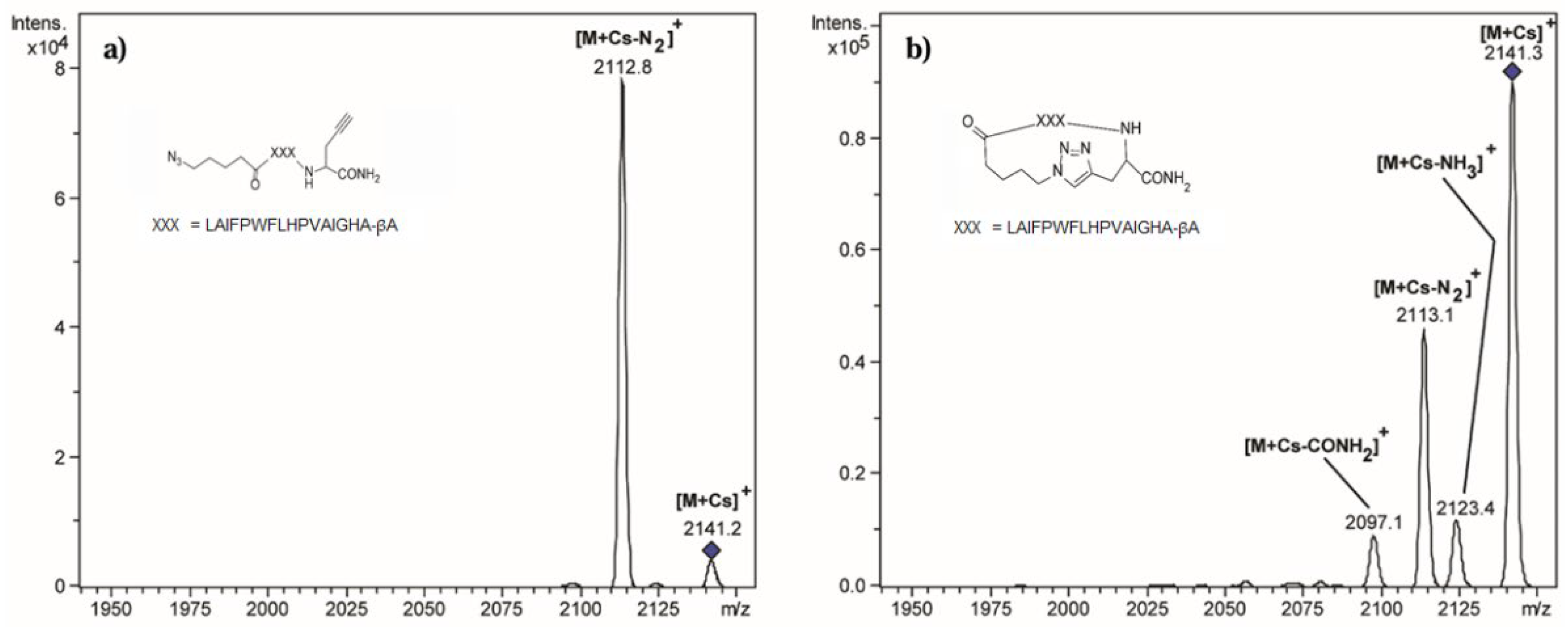
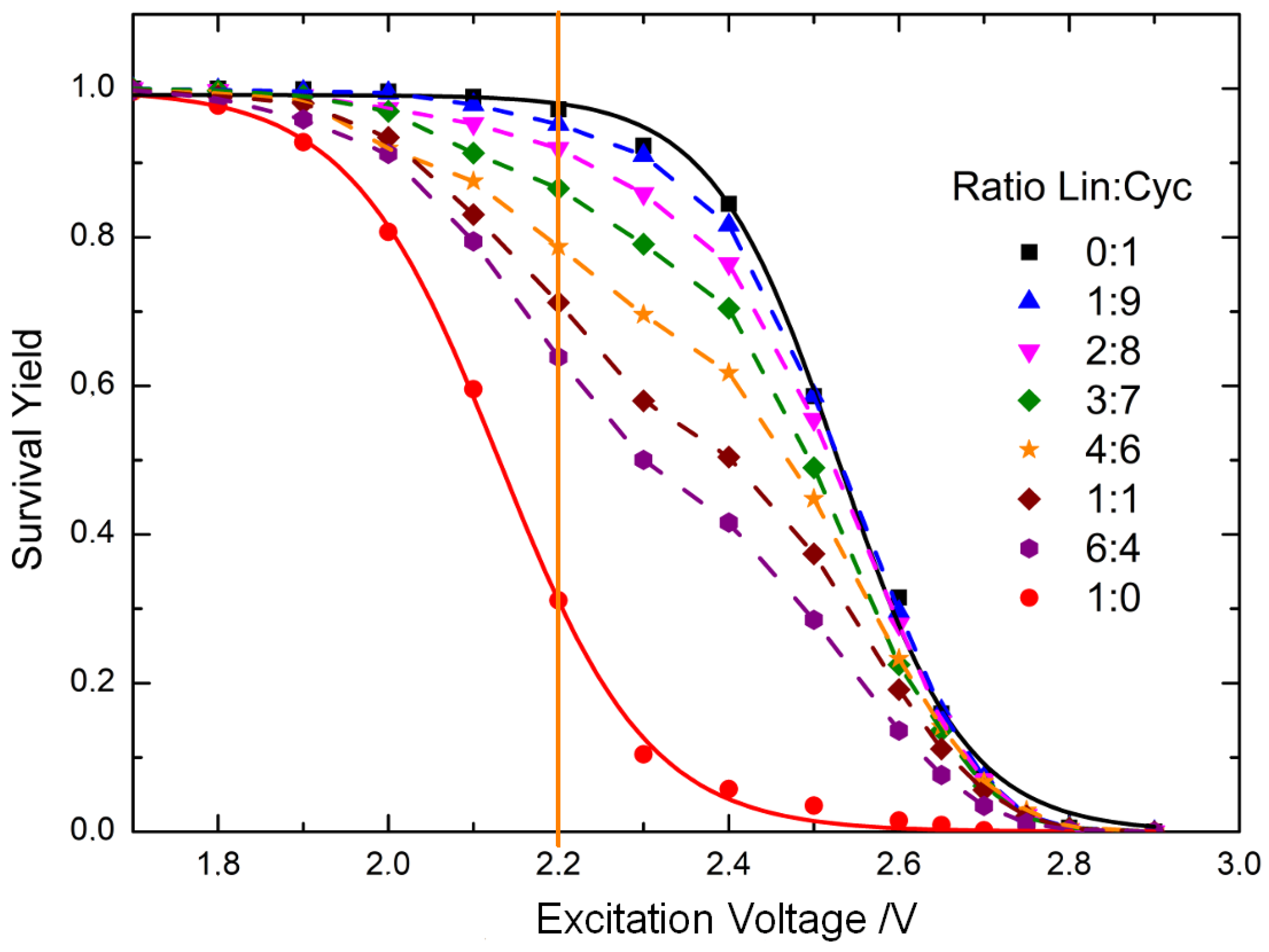
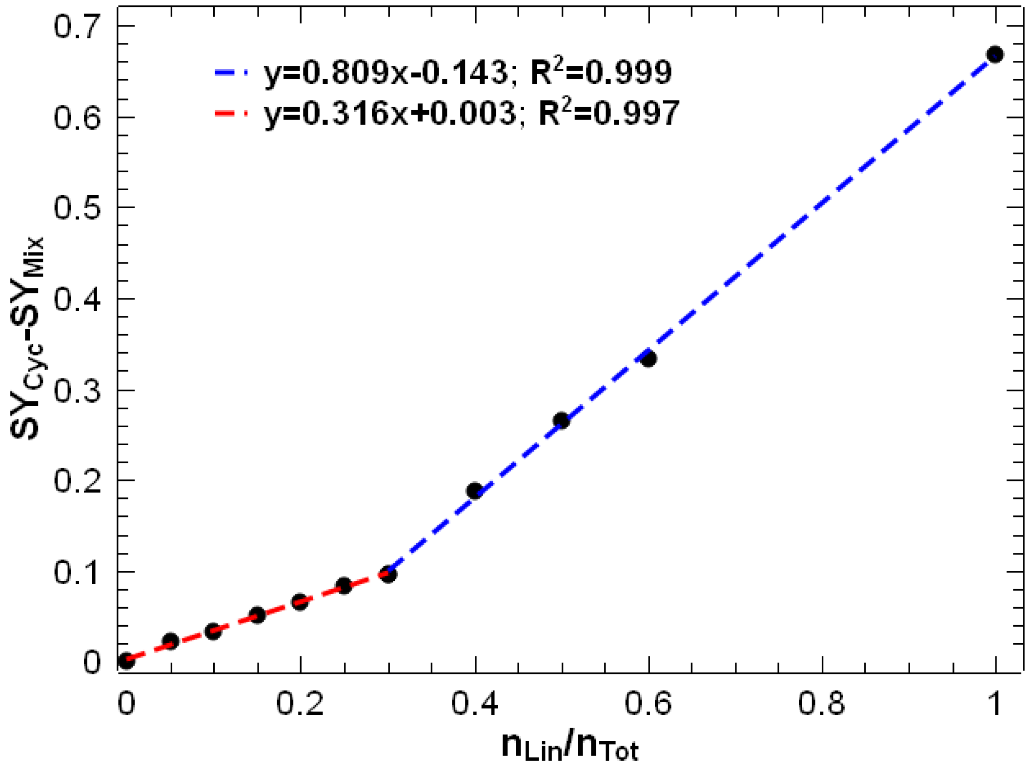
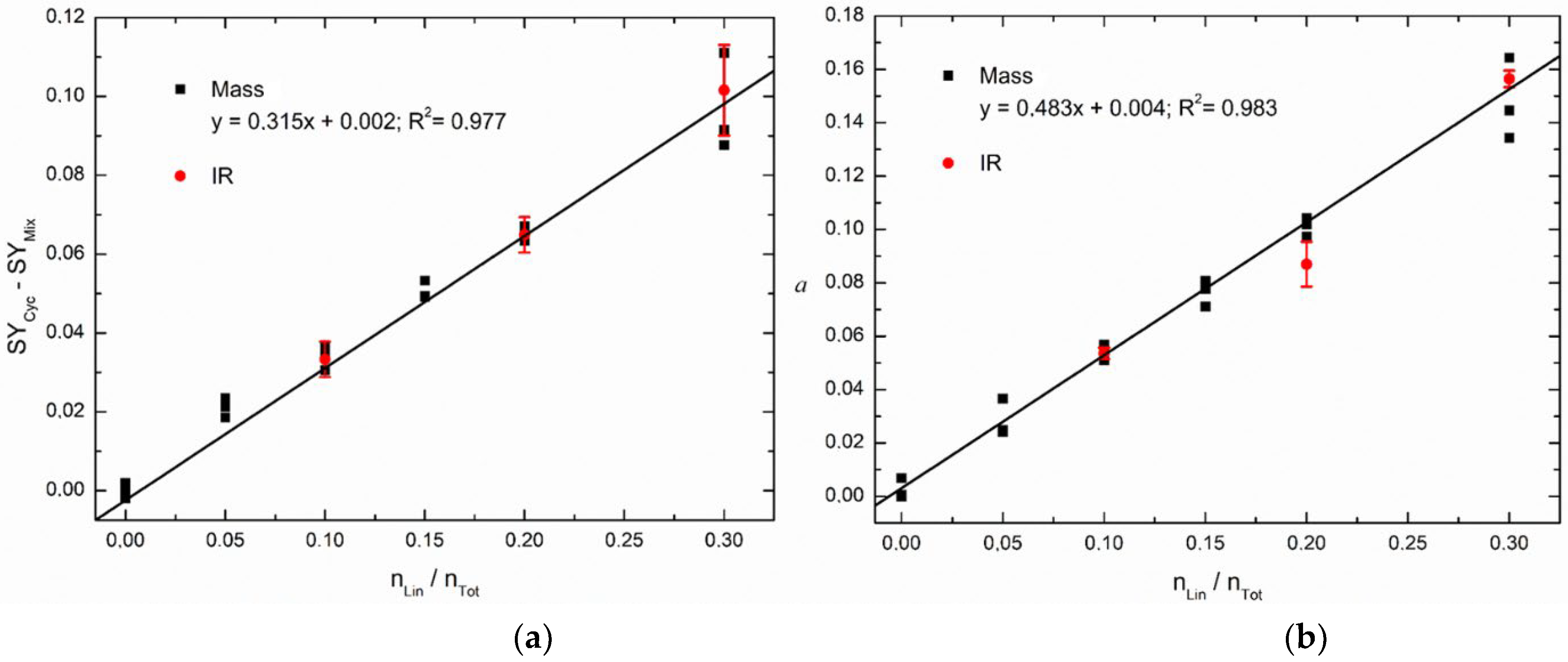
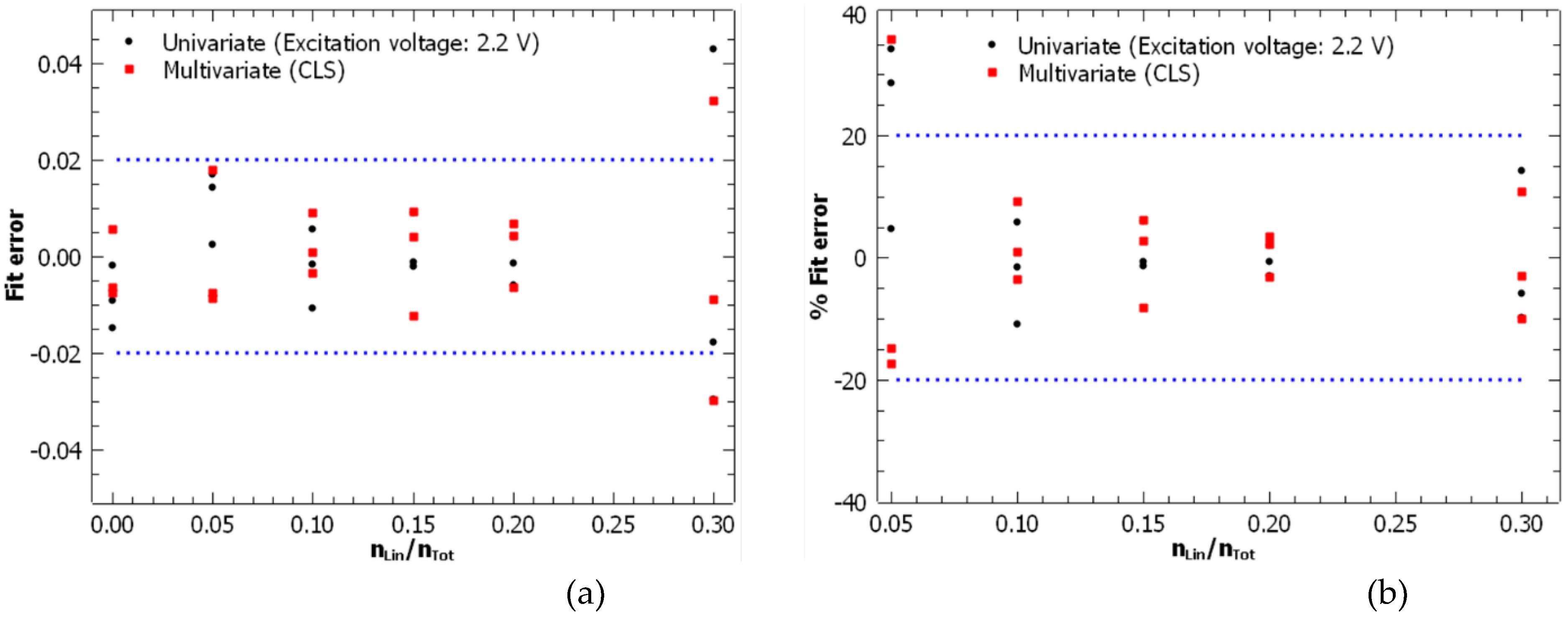
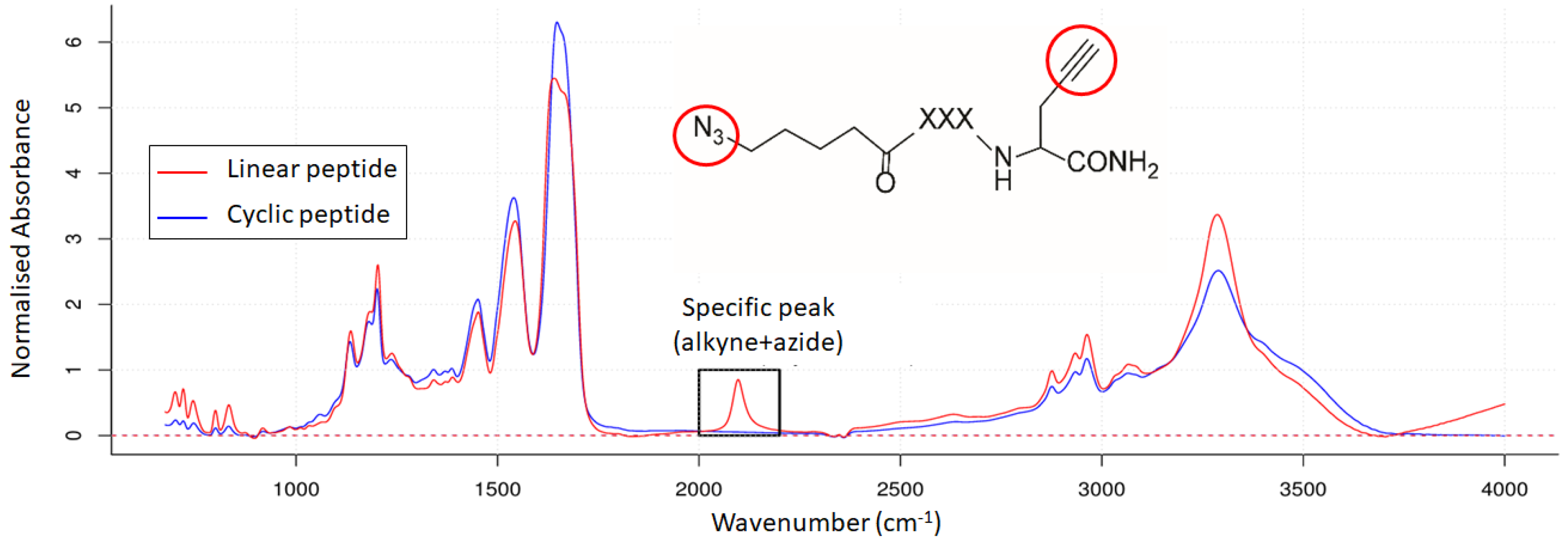
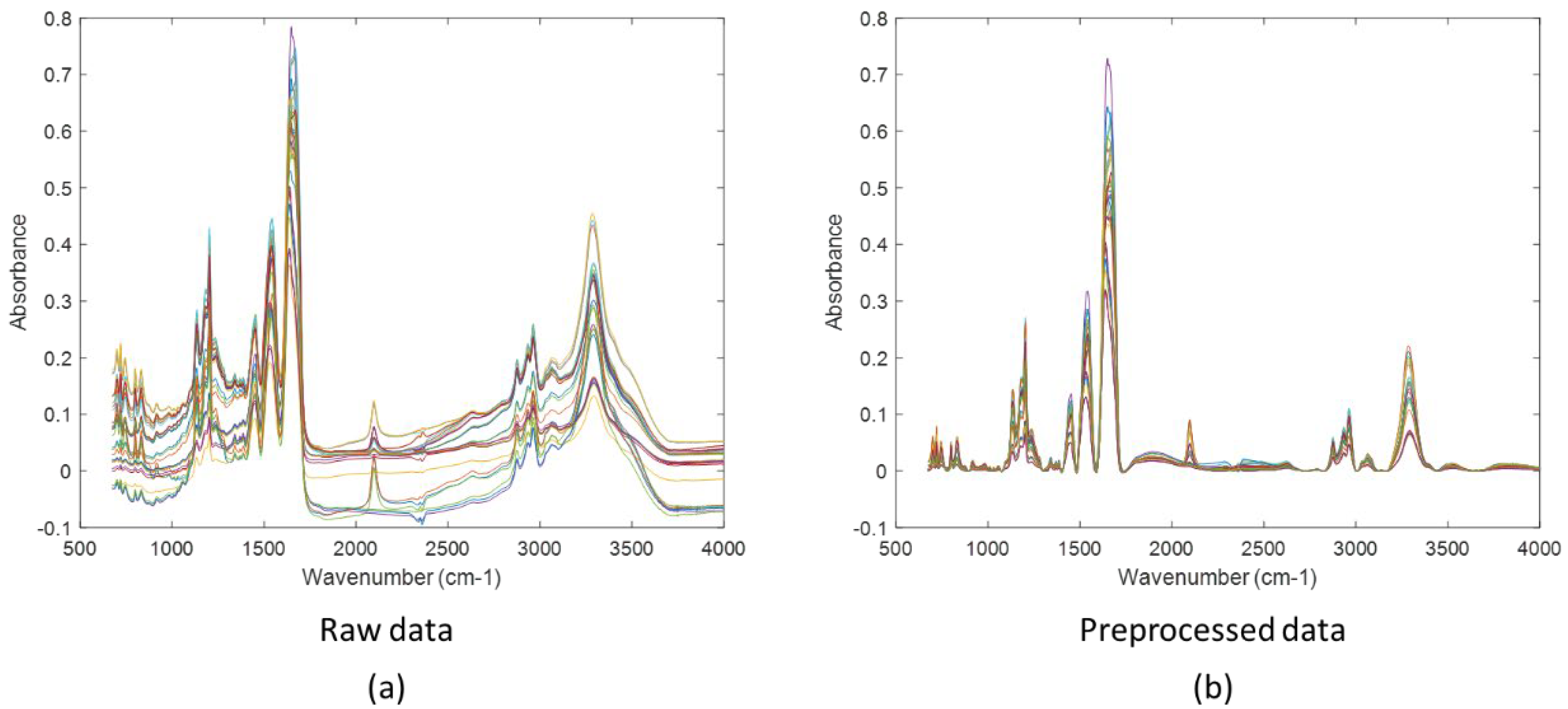
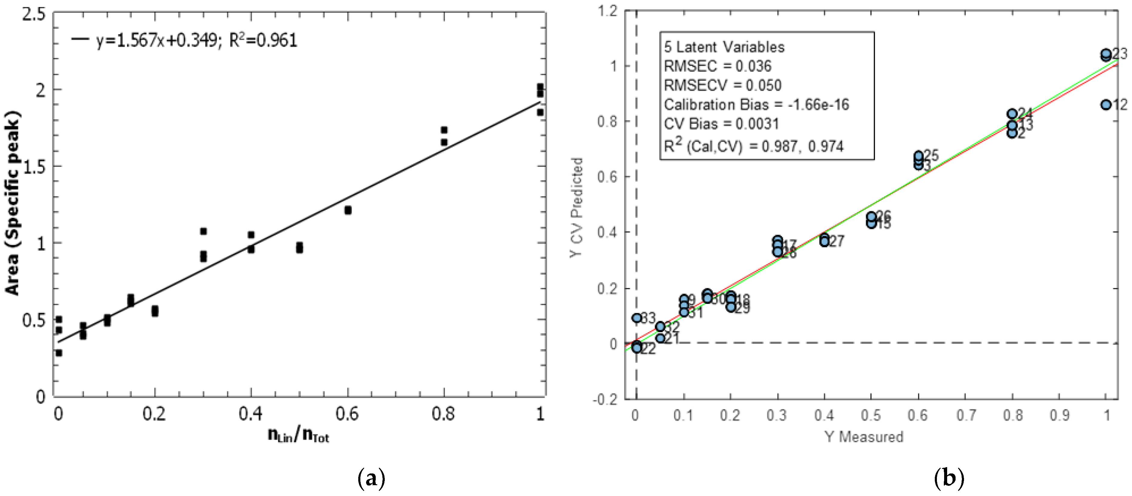
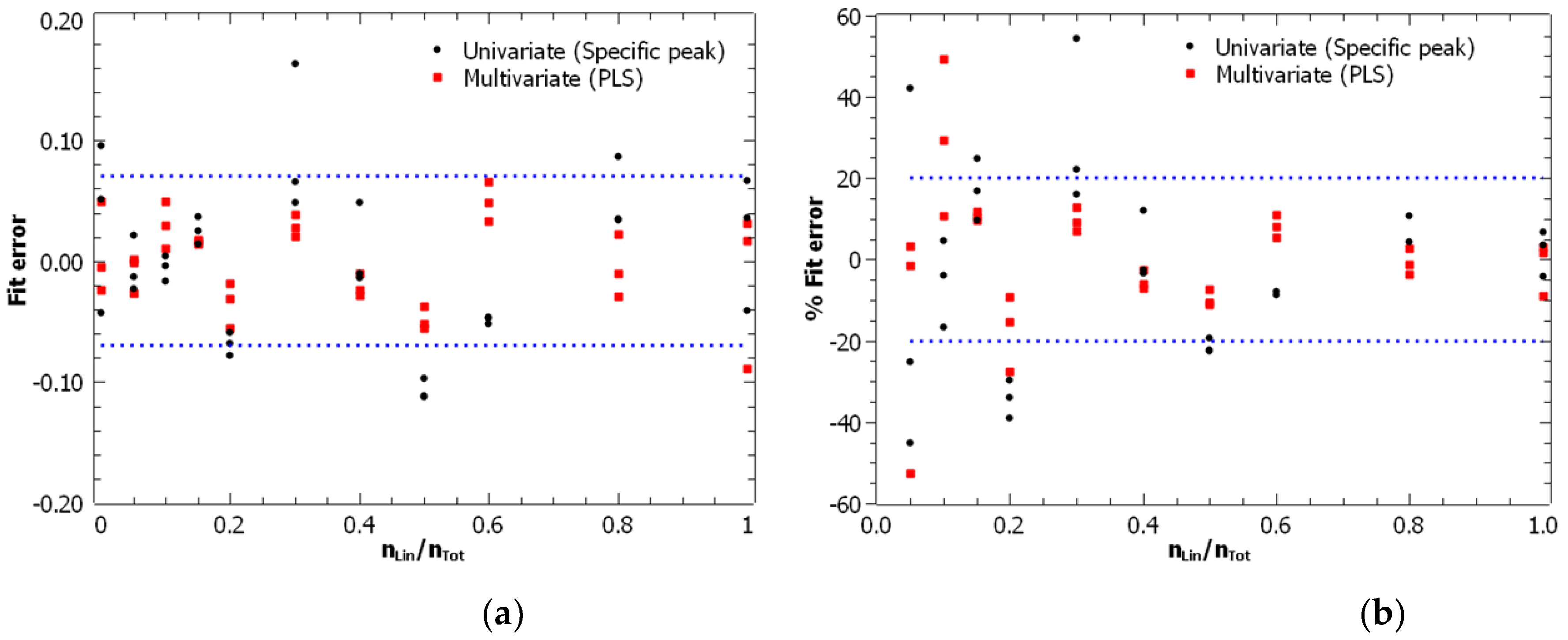
| Analytical technique | Calibration model | Linearity interval |
R2 | Fit error (RMSEC) |
Intermediate precision | Detection limit (LD) |
|---|---|---|---|---|---|---|
|
ER MS |
Univariate | 0 - 0.3 | 0.977 | 0.015 | 1.71·10-2 | 0.053 |
| Multivariate (CLS) | 0 - 0.3 | 0.983 | 0.013 | 1.58·10-2 | 0.045 | |
| IR microscopy |
Univariate | 0 - 1 | 0.961 | 0.062 | 5.06·10-2 | 0.21 |
| Multivariate (PLS) | 0 - 1 | 0.987 | 0.036 | 2.63·10-2 | 0.11 |
Disclaimer/Publisher’s Note: The statements, opinions and data contained in all publications are solely those of the individual author(s) and contributor(s) and not of MDPI and/or the editor(s). MDPI and/or the editor(s) disclaim responsibility for any injury to people or property resulting from any ideas, methods, instructions or products referred to in the content. |
© 2024 by the authors. Licensee MDPI, Basel, Switzerland. This article is an open access article distributed under the terms and conditions of the Creative Commons Attribution (CC BY) license (http://creativecommons.org/licenses/by/4.0/).


