Submitted:
30 September 2024
Posted:
03 October 2024
You are already at the latest version
Abstract
Keywords:
1. Introduction
2. Related Works
2.1. Prophet Model
2.2. GRU(Gated Recurrent Unit)
3. Problem Definition and Solution Methods
3.1. Prophet Model’s Problem
3.2. Solution Methods
4. Proposed Methods
4.1. Data Collection
4.1.1. Solar PV System Install Location
4.1.2. Power Generation and Meteorological Data
4.2. Data Pre-Processing
4.3. Data Partition for Training and Test Data
4.4. Modified Prophet Model
| Parameter Nature | Parameter Name | Value |
|---|---|---|
| Trend Parameters | growth | linear |
| changepoints | None | |
| n_changepoints | 25 | |
| changepoint_range | 0.8 | |
| changepoint_prior_scale | 0.01 | |
| Seasonality parameters | yearly_seasonality | 10 |
| weekly_seasonality | False | |
| daily_seasonality | False | |
| seasonality_mode | multiplicative | |
| seasonality_prior_scale | 10 | |
| holidays parameters |
Holidays holidays_prior_scale |
df 0.25 |
| Flow parameters | flow | flow |
| flow_prior_scale | 10 | |
| Other parameters | mcmc_samples | 0 |
| interval_width | 0.8 |
4.5. Proposed Hybrid Model
5. Simulation Metrics and Results
5.1. Simulation Metrics
5.2. Simulation Results
6. Conclusion
Author Contributions
Funding
Institutional Review Board Statement
Informed Consent Statement
Data Availability Statement
Acknowledgments
Conflicts of Interest
References
- The Presidential Commission on Carbon Neutrality and Green Growth. 2050 Presidential Commission on Carbon Neutrality and Green Growth. 2030 Nationally Determined Contributions. Policy Report, Sejong-si, Republic of Korea, 2021.
- International Energy Agency; Renewable Energy Market Update. International Energy Agency, 2023, Paris, France.
- Lee, S.H.; Cho, I.H. International Renewable Energy Policy Change and Market Analysis. Korea Energy Economics Institute, 2018, Seongan-dong, Korea.
- Rethink Energy-Solar Service. Solar Industry growing rapidly with DER skew post-pandemic., Rethink Energy, Mar. 29, 2023.
- European Commission. EU strategic dependencies and capacities: second stage of in-depth reviews. Feb. 2, 2022.
- Huang, B.B.; Zhang, Y.Z.; Wang, C.X. Judgment of China’s 14th five-year plan new energy development and issues needing attention. Electr. Power 2020, 53, 1089–1094. [Google Scholar]
- Korea Energy Economics Institute (KEEI). Modified CFI 2030 Plan to Implement Energy Self-Reliance Island. KEEI: Ulsan, Korea, 2019.
- Noh, C.H.; Jang, W.H.; Kim, C.H. Recent Trends in Renewable Energy Resources for Power Generation in the Republic of Korea. Resources. 2015, 4, 751–764. [Google Scholar] [CrossRef]
- Rashid, M.M.U.; Granelli, F.; Hossain, M.A.; Alam, M.S.; Alismail, F.S.; Karmaker, A.K.; Rahaman, M.M. Development of Home Energy Management Scheme for a Smart Grid Community. Energies 2020, 13, 4288. [Google Scholar] [CrossRef]
- Raza, M.Q.; Khosravi, A. A review on artificial intelligence based load demand forecasting techniques for smart grid and buildings. Renew. Sustain Energy Rev. 2015, 50, 1352–1372. [Google Scholar] [CrossRef]
- Willis, H.L.; Northcote-Green, J.E.D. Spatial electric load forecasting: A tutorial review. Proc. Of the IEEE 1983, 71, 232–253. [Google Scholar] [CrossRef]
- Enea, M. A review of machine learning algorithms used for load forecasting at micro-grid level. In Sinteza 2019—International Scientific Conference on Information Technology and Data Related Research, Singidunum University, Belgrade, Serbia, pp.452–458, 2019.
- Brown, R.G. Smoothing Forecasting and Prediction of Discrete Time Series; Prentice-Hall: Englewood Cliffs, NJ, USA, 1963. [Google Scholar]
- Ohtsuka, Y.; Oga, T.; Kakamu, K. Forecasting electricity demand in Japan: A Bayesian spatial autoregressive ARMA approach. Comput. Stat. Data Anal. 2010, 54, 2721–2735. [Google Scholar] [CrossRef]
- Fix, E.E.; Hodges, J.L., Jr. Discriminatory Analysis-Nonparametric Discrimination: Consistency Properties; International Statistical Institute: Voorburg, The Netherlands, 1989; Vol. 57, pp. 238–247. [Google Scholar] [CrossRef]
- Yu, Z.; Haghighat, F.; Fung, B.C.M.; Yoshino, H. A decision tree method for building energy demand modeling. Energy Build 2010, 42, 1637–1646. [Google Scholar] [CrossRef]
- Dong, B.; Cao, C.; Lee, S.E. Applying support vector machines to predict building energy consumption in tropical region. Energy Build. 2005, 37, 545–553. [Google Scholar] [CrossRef]
- Bonyadi, M.R.; Michalewicz, Z. Particle swarm optimization for single objective continuous space problems: A review. Evol. Comput. 2017, 25, 1–54. [Google Scholar] [CrossRef]
- Kalogirou, S.A; Neocleous, C.C; Schizas, C.N. Building heating load estimation using artificial neural networks. In Proceedings of the 17th International Conference on Parallel Architectures and Compilation Techniques, San Francisco, CA, USA, 10–14 November 1997. [Google Scholar]
- Freedman, D.A. Statistical Models: Theory and Practice; Cambridge University Press, 2009; Volume 26. [Google Scholar]
- Bagnasco, A.; Fresi, F.; Saviozzi, M.; Silvestro, F.; Vinci, A. Electrical consumption forecasting in hospital facilities: An application case. Energy Build. 2015, 103, 261–270. [Google Scholar] [CrossRef]
- Graves, A.; Liwicki, M.; Fernandez, F.; Bertolami, R.; Bunke, H.; Schmidhuber, J. A Novel Connectionist System for Improved Unconstrained Handwriting Recognition. IEEE Trans. Pattern Anal. Mach. Intell. 2009, 31, 855–868. [Google Scholar] [CrossRef] [PubMed]
- Gers, F.; Schmidhuber, J.; Cummins, F. Learning to Forget: Continual Prediction with LSTM. In Proceedings of the 9th International Conference on Artificial Neural Networks, ICANN’99, Edinburgh, UK, 7–10 September 1999; pp. 850–855. [Google Scholar]
- Ian, G.; Yoshua, B.; Aaron, C. Deep Learning; MIT Press: Cambridge, MA, USA, 2016. [Google Scholar]
- Valenzuela, P.; Gorricho, J.; Iglesia, D.L. Automatic model and feature selection for time series forecasting: Achieving good performance and interpretability. Information Sciences 2018, 157–174. [Google Scholar]
- Sanguansat, E.; Klomjit, N. A comparative study of machine learning techniques for short-term load forecasting. Energies 2019, 12. [Google Scholar]
- Fung, G.; Shih, E. Evaluating the Forecasting Performance of Facebook's Prophet Model for Time Series Data. Journal of Open Source Software 2019, 4. [Google Scholar]
- Bashir, B.; Haoyong, C. Short-term electricity load forecasting using hybrid prophet-LSTM model optimized by BPNN. Energy Reports 2022, 8, 1678–1686. [Google Scholar] [CrossRef]
- Arslan, S. A hybrid forecasting model using LSTM and Prophet for energy consumption with decomposition of time series data. PeerJ Computer Science 2022, 8. [Google Scholar] [CrossRef]
- Pin, L.; Zhang, J.S. A New Hybrid Method for China’s Energy Supply Security Forecasting Based on ARIMA and XGBoost. Energies 2018, 11. [Google Scholar]
- Yuanhua, C.; Muhammad, S.B.; Muhammad, A.; Dingtian, X. Evaluation of Machine Learning Models for Smart Grid Parameters: Performance Analysis of ARIMA and Bi-LSTM. Sustainability 2023, 15. [Google Scholar] [CrossRef]
- Pooniwala, N.; Sutar, R. Forecasting Short-Term Electric Load with a Hybrid of ARIMA Model and LSTM Network. International Conference on Computer Communication and Informatics, 2021.
- Agbessi, A.P.; Salami, A.A.; Agbosse, K.S.; Birregah, B. Peak Electrical Energy Consumption Prediction by ARIMA, LSTM, GRU, ARIMA-LSTM and ARIMA-GRU Approaches. Energies 2023, 16. [Google Scholar] [CrossRef]
- Taylor, S.J.; Letham, B. Prophet: forecasting at scale. Proceedings of the 22nd ACM SIGKDD International Conference on Knowledge Discovery and Data Mining, pp.1389-1397, 2017.
- Taylor, S.J.; Letham, B. Prophet: forecasting at scale. Proceedings of the 22nd ACM SIGKDD International Conference on Knowledge Discovery and Data Mining, pp.1389-1397, 2017.
- Cho, K.; Merriënboer, B.V.; Bahdanau, D.; Bengio, Y. On the properties of neural machine translation: Encoder-decoder approaches. Proceedings of SSST-8, Eighth Workshop on Syntax, Semantics and Structure in Statistical Translation, 2014.
- Work Calendar Library Package. Available online: https://pypi.org/project/workalendar/ (accessed on 20 August 2024).
- Namrye, S.; Mina, J. Analysis of Meteorological Factor Multivariate Models for Medium- and Long-Term Photovoltaic Solar Power Forecasting using Long Short-Term Memory. Applied Sciences 2021, 11, 316. [Google Scholar]
- Robust Scaler Documentation in Scikit-Learn. Available online: https://www.itl.nist.gov/div898/software/dataplot/refman2/auxillar/iqrange.htm (accessed on 20 August 2024).
- Kingma, D.; Ba, J. Adam: A method for stochastic optimization. arXiv 2015, arXiv:1412.6980. [Google Scholar]
- Nair, V.; Hinton, G. Rectified linear units improve restricted Boltzmann machines. In Proceedings of the 27th International Conference on International Conference on Machine Learning, Haifa, Israel, 21–24 June 2010. [Google Scholar]
- Sethna, J.P. Chapter 10: Correlations, response, and dissipation. In Statistical Mechanics: Entropy, Order Parameters, and Complexity; Oxford University Press: Oxford, UK, 2006; ISBN 978-0198566779. [Google Scholar]
- RMSE. Available online: https://en.wikipedia.org/wiki/Root_mean_square_deviation (accessed on 20 August 2024).
- RMSSE. Available online: https://www.pmorgan.com.au/tutorials/mae%2C-mape%2C-mase-and-the-scaled-rmse/ (accessed on 20 August 2024).
- SMAPE. Available online: https://en.wikipedia.org/wiki/Symmetric_mean_absolute_percentage_error (accessed on 20 August 2024).
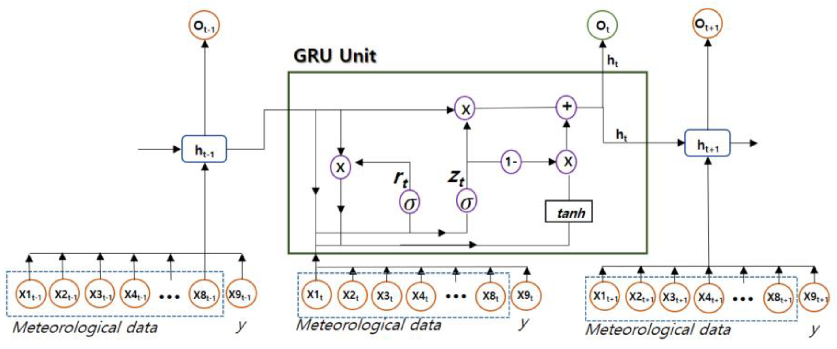
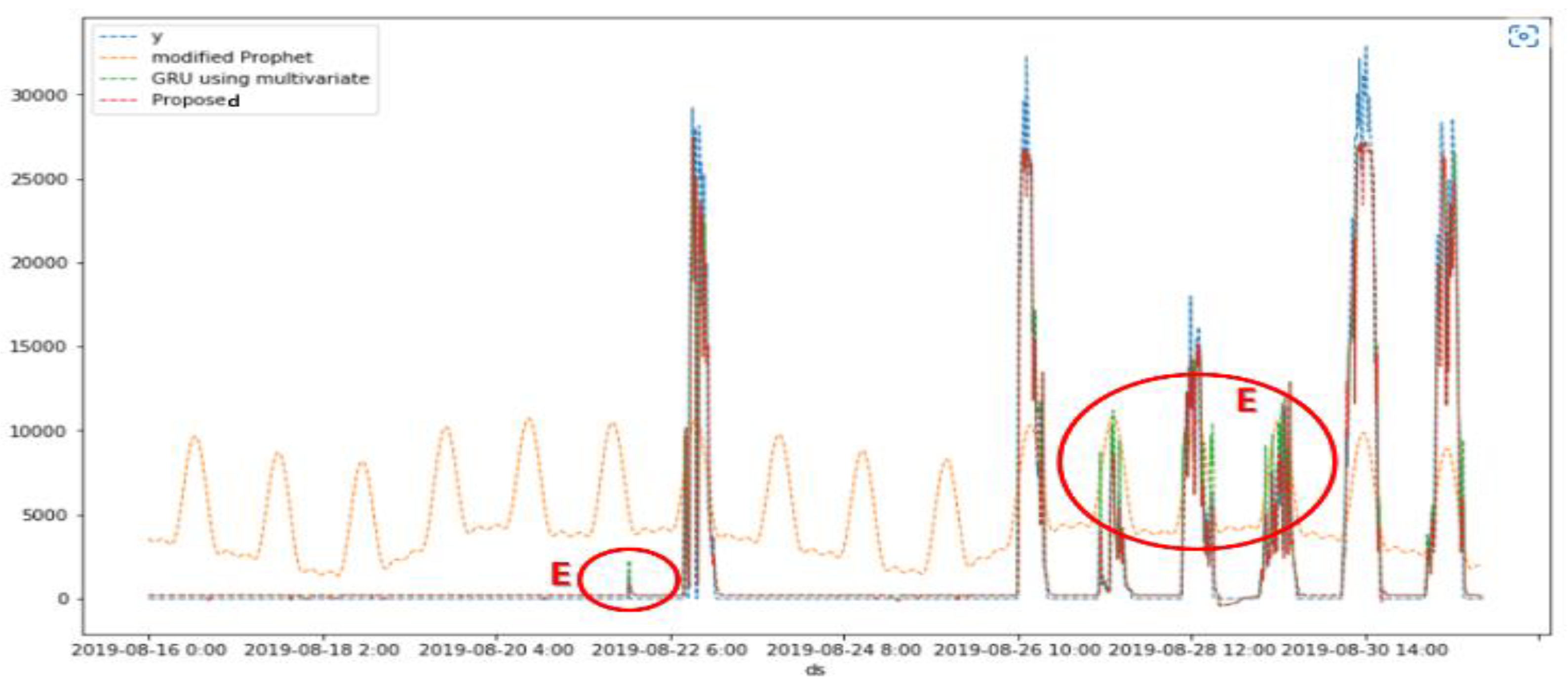
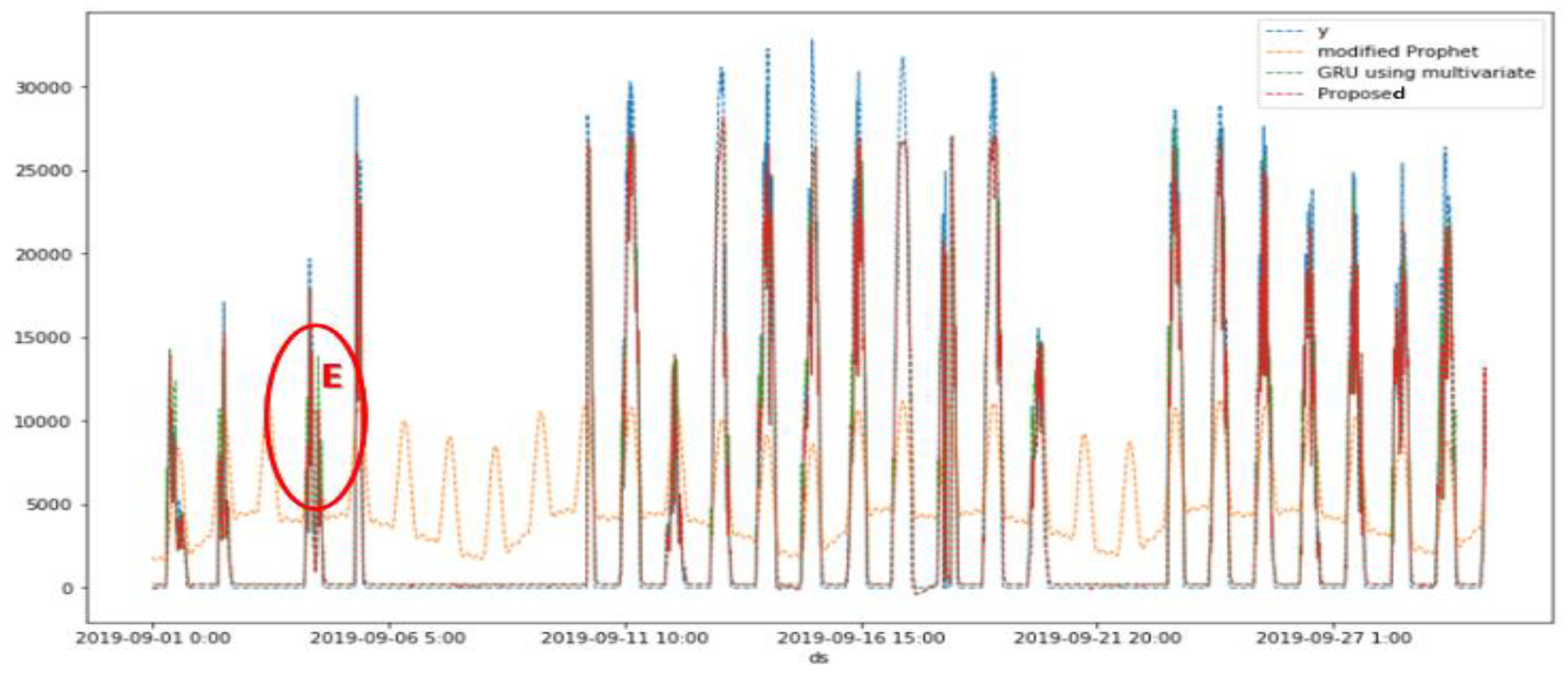
| Division | Information |
| Location | Naju, Jeollanam-do, South Korea |
| The main purpose of usage | Self-generated solar power generation |
| Building area | Total 3 building, 600,983m2 |
| Number of floors | 1st floor of the factory building and one other building |
| Building structure | H-beam |
| Outer wall | Sandwich panels |
| PV system capacity | 50KW |
| ESS | PCS: 100KW, battery: 200KW |
| Parameter | GRU |
| Number of layers | 9 |
| Number of neurons | 9 |
| Number of epochs | 500 |
| Learning rate | 0.005 |
| Loss function | MSE |
| Optimization | ADAM |
| Weight initializer | 1 |
| Activation function | ReLU |
| Term | Metrics | Modified Prophet |
GRU using multivariate |
Proposed | |
|---|---|---|---|---|---|
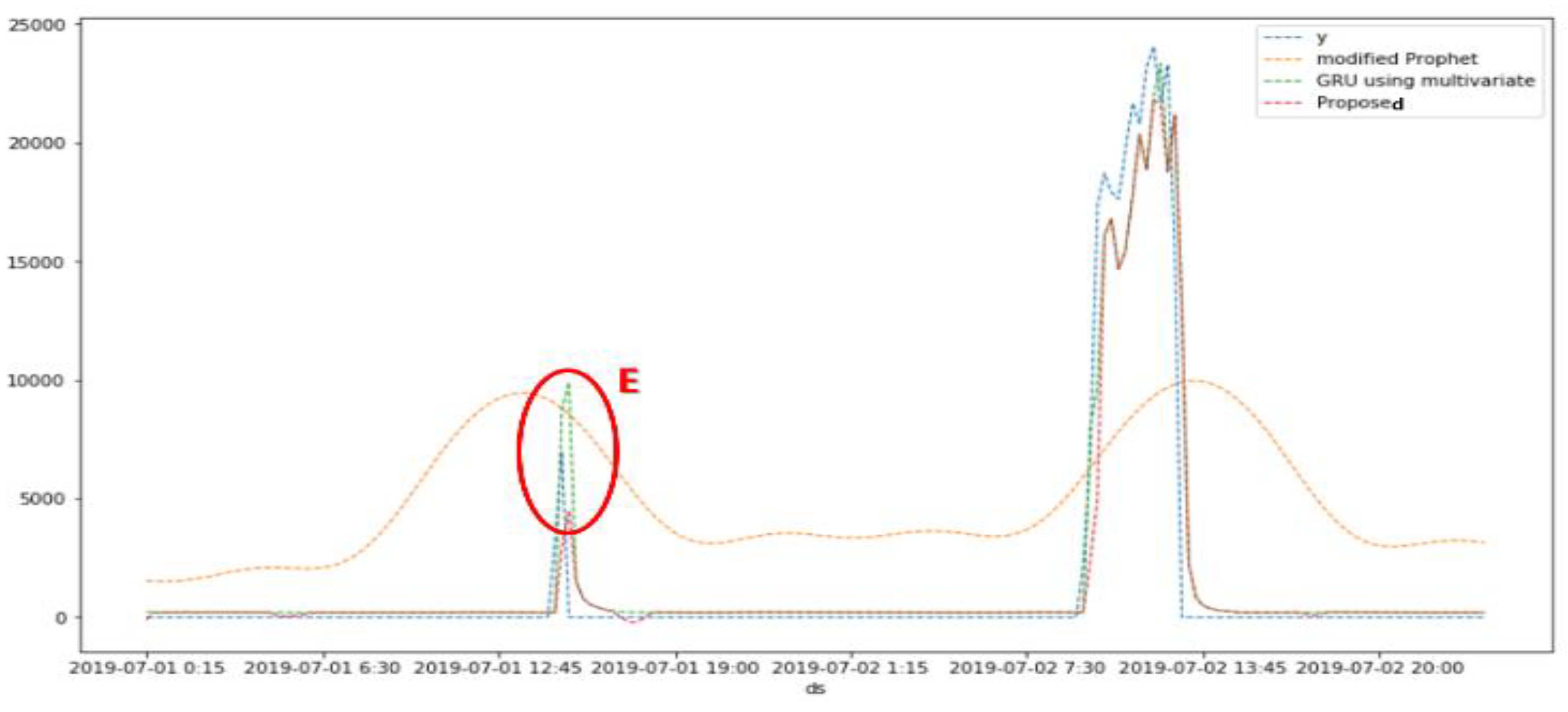
| Short- term |
2 days (July 1~2) |
CC | 0.39 | 0.94 | 0.95 |
| RMSE | 5765.38 | 1660.25 | 1588.59 | ||
| RMESE | 36732.30 | 10577.77 | 10121.23 | ||
| SMAPE (%) | 189.47 | 187.43 | 186.45 | ||
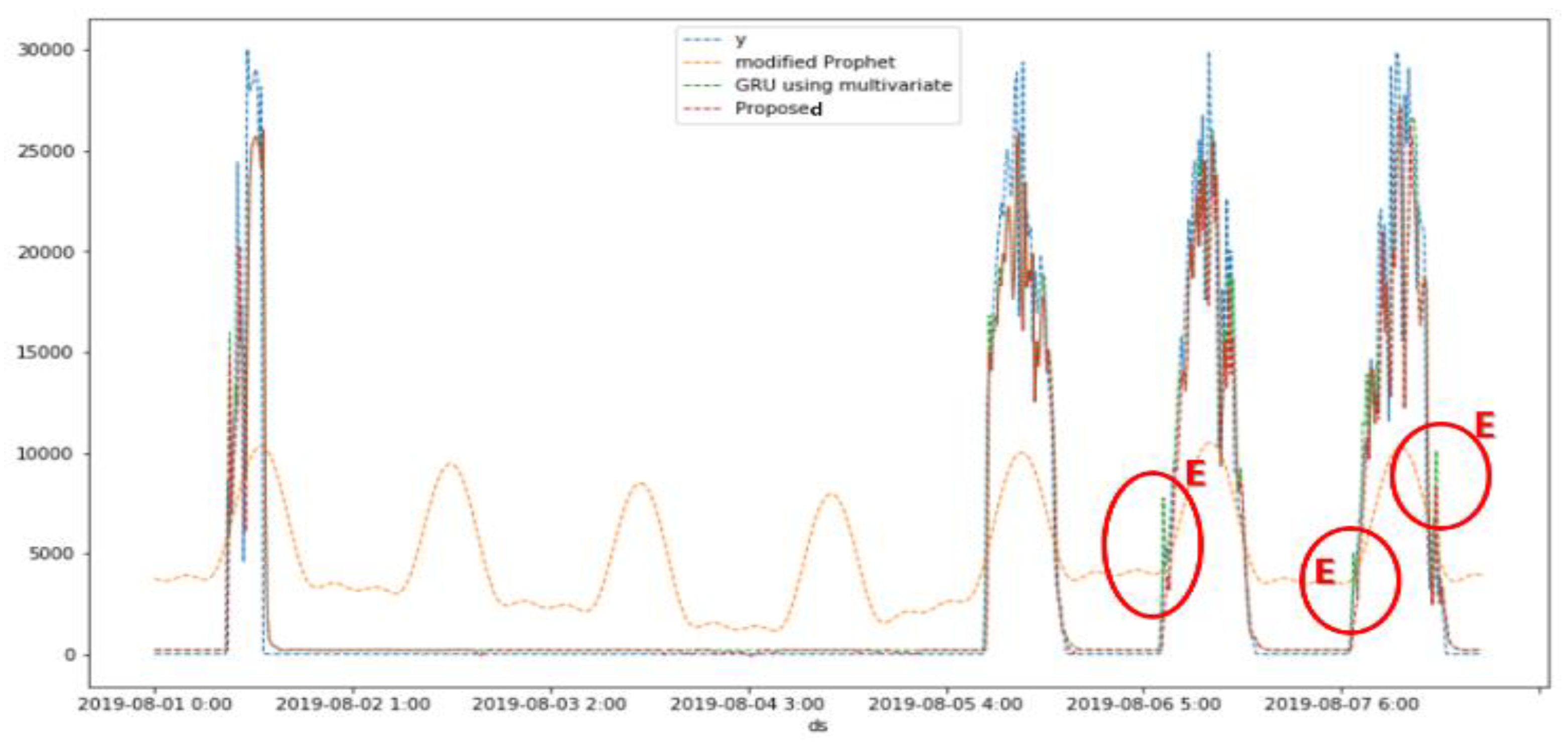
| 7 days (Aug. 1~7) |
CC | 0.69 | 0.95 | 0.95 | |
| RMSE | 6393.15 | 2521.99 | 2510.73 | ||
| RMSSE | 76202.52 | 30060.66 | 29926.40 | ||
| SMAPE (%) | 169.36 | 160.89 | 160.38 | ||
| Medium- term |
15 days ( Aug. 16~30) |
CC | 0.47 | 0.96 | 0.96 |
| RMSE | 6141.05 | 1822.63 | 1756.73 | ||
| RMSSE | 110664.40 | 32844.71 | 31657.08 | ||
| SMAPE (%) | 177.34 | 170.66 | 170.62 | ||
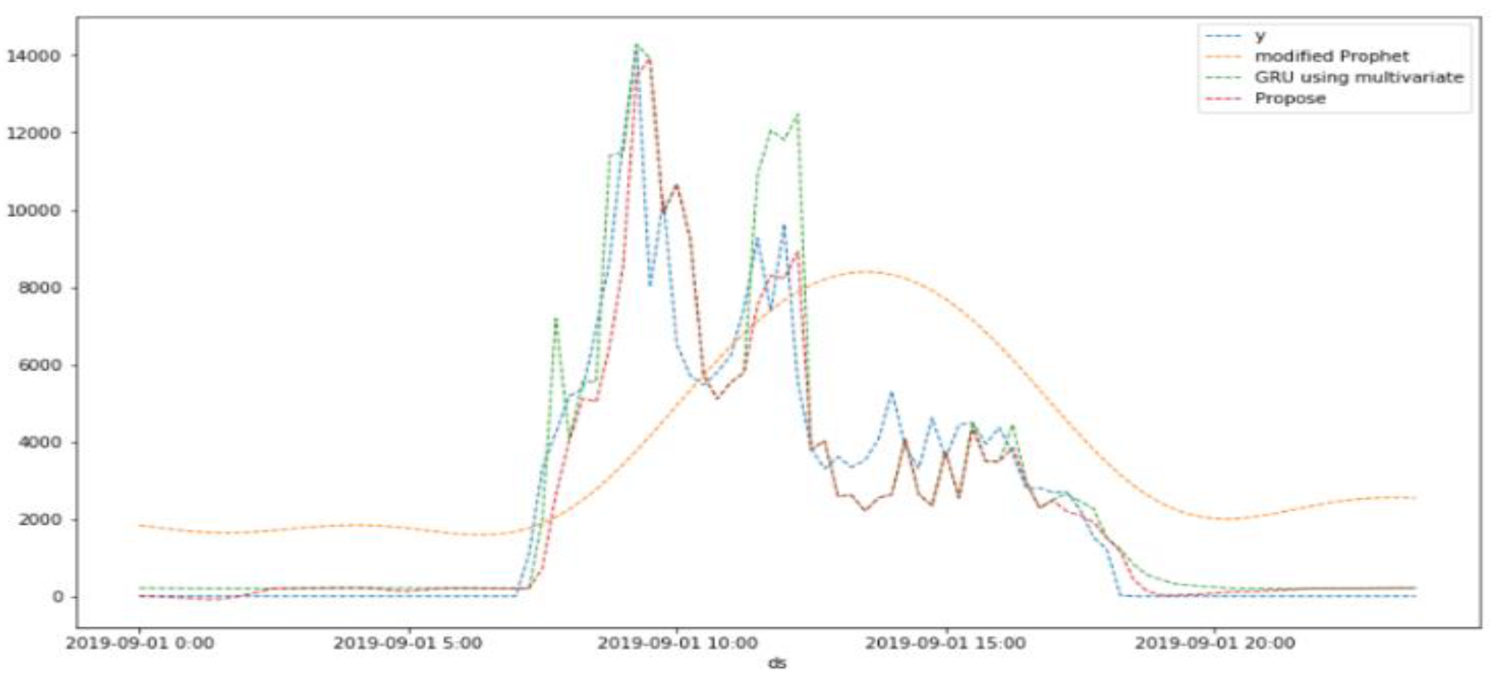
| 30 days (Sep. 1~30) |
CC | 0.67 | 0.96 | 0.96 | |
| RMSE | 6601.82 | 2272.38 | 2227.31 | ||
| RMSSE | 161311.70 | 55524.48 | 54423.11 | ||
| SMAPE (%) | 158.2 | 146.84 | 146.70 | ||
Disclaimer/Publisher’s Note: The statements, opinions and data contained in all publications are solely those of the individual author(s) and contributor(s) and not of MDPI and/or the editor(s). MDPI and/or the editor(s) disclaim responsibility for any injury to people or property resulting from any ideas, methods, instructions or products referred to in the content. |
© 2024 by the authors. Licensee MDPI, Basel, Switzerland. This article is an open access article distributed under the terms and conditions of the Creative Commons Attribution (CC BY) license (http://creativecommons.org/licenses/by/4.0/).


