1. Introduction
Conventional monitoring strategies in electrical power systems rely on the measured root mean square (RMS) voltages, currents, and power (active, reactive, and apparent). Phasor measurement units (PMUs) provide additional information about the relative voltage phasor’s magnitude and angle. For power flow (PF) analysis, a measurement resolution of 15-minute steps is typical and sufficient in most use cases. When it comes to measurements of power quality (PQ), various time intervals need to be considered. By definition, PQ is assessed through any deviation in the voltage’s waveform from an ideal sinusoidal shape at an expected RMS voltage with a stable fundamental frequency [
1]. Typical PQ disturbances are voltage sags or swells, flickers, harmonics, or short-period transient deformations. Characteristics for PQ are already considered in a wide range of standards (e.g., European EN50160 or EN61000-2-2). These standards necessitate the analysis of various parameters over time intervals ranging from milliseconds to hours [
2,
3].
PQ meters provide all relevant RMS values, voltage- and current phasors, various harmonic levels, flicker-evaluation, and high-resolution oscilloscope records to capture transient disturbances. Time-synchronizing these measurements via precision time protocol (PTP) or Global Positioning System (GPS) enables applications like wide area monitoring systems (WAMS) [
4]. WAMSs can be used to acquire the necessary data for PQ state estimation (PQSE), which describes various state estimation (SE) techniques for different PQ issues [
5].
Assuming that a high penetration of distributed generation and electric vehicle charging in low- (LV) or medium-voltage (MV) grids influences PQ significantly, research and simulations have been conducted to quantify this impact. The authors in [
6] prove a strong contribution of large photovoltaic (PV) systems to harmonic distortion in Columbian distribution grids. Other sources discuss how smaller systems affect PQ. Using a simulation model, [
7] shows that PV systems connected to LV grids may cause considerable transient effects, voltage sags, and harmonics. [
8] analyzes the influence of electric vehicle charging in LV grids on technical equipment such as transformers. The authors propose to limit the current total harmonic distortion (THD) to
to preserve a reasonable life expectancy, as harmonic currents cause premature aging of components. Yet, another work observes current THD of up to
for powerful, commercially available electric vehicle supply equipment (EVSE) of older generations [
9]. Typically, the THD is defined as follows in (
1). In these works, and also in [
10] the THD is defined up to the 50
th order. Nevertheless, the highest order considered may vary depending on the application.
Considering these influences on grid operation, distribution grid operators have an incentive to assess the current level of harmonics and to identify the origins of PQ disturbances.
Therefore, this paper presents a high-performance estimation method suitable for application in near-real-time environments. Typically, this term is defined based on the specific application and refers to the system’s processing time from the initiation of an event to the completion of transmission and evaluation [
11]. In harmonic analysis, the shortest evaluation interval commonly used determines the performance requirements for SE. For example, the IEEE519 standard requires evaluation of voltage harmonics with an average interval of 3 seconds [
10]. The developed algorithm provides results within this time frame.
2. State of the Art
Harmonic state estimation (HSE) generates knowledge about harmonic quantities at unmeasured locations based on a specific set of measurements. A few algorithms for HSE in LV and MV grids can be found in the current literature. The following will give an overview of known methods for HSE in distribution grids and the benchmark advantages of data-driven algorithms in this field.
2.1. Harmonic State Estimation for Distribution Grids
Most of the algorithms are based on iterative processes, which are computationally expensive and require a large number of meters to achieve decent observability of the grids’ states. We will examine these aspects in detail in the results section of this article. Some of these conventional methods for HSE are, e.g., the weighted least squares (WLS) approach [
12], the method of singular value decomposition (SVD), which is a derivate of the WLS for sparse measurement infrastructure [
13,
14], or the Kalman filter (KF), which iterates over a time series of states to converge [
15].
2.2. Neural Networks for State Estimation
To highlight the difficulty of conventional iterative methods in maintaining observability with a small number of measurement devices, an example from [
16] of a PF-SE based on WLS is presented. In this example, a distribution system is stated as unobservable with 31 buses and 21 meter locations.
Completely different scenarios are possible when applying data-driven methods, as demonstrated in [
17]. This work performs a PF-SE by using an artificial neural network (ANN) in a 32-node distribtion grid, which is observed by only three PMU measurements. This underscores the potential benefits of adopting more advanced statistical techniques, such as ANNs, for PQSE.
Another machine learning-based approach for SE is discussed in [
18]. Here, an ANN is presented to apply PF-SE on a UK 95-bus network. The maximum time for estimating a system state among 88 samples was
, while a range of non-data-driven works reported execution times of nearly a minute or more for convergence [
12,
19,
20,
21]. This highlights ANN applications for near-real-time computation tasks, too.
Accurate results for an ANN and simulation-based HSE considering the first 13 harmonic orders are presented in [
22]. The author’s concept takes probabilistic distributions of load and PV systems into account while processing smart meter data and sparse PMU measurements. A different approach based on ANNs is presented in [
23]. Here, a generative adversarial network (GAN) is implemented. This combination of two ANNs is utilized for HSE and yields accurate results compared to a KF implementation.
[
24] used a method of pruning connections in a dense ANN (DNN) to integrate physical knowledge of the grid’s topology into the data model. This ANN architecture is known as physics-aware ANN (PANN) and will be applied in this work to incorporate information about infrastructure like connection dependencies of cables and transformers. According to [
24], this method is especially suited for applications with a low coverage of measurements. The authors of this study demonstrate robust and precise estimation of fundamental frequency voltage phasors for distribution grids. The authors in [
25] published the basis for the work in [
24] and showed very short execution times for predictions with their PANN. Merely,
were needed to estimate the PF for 37 buses. Compared to DNNs, the PANN is resilient against overfitting and vanishing or exploding gradients. The SE accuracy in comparison to traditional iterative methods is better for almost every tested scenario. Especially when sparse meter coverage impedes convergence for conventional algorithms, the PANNs still provide very good SE results. Since the static structure of the distribution grid is integral to the ANN architecture, a trained model requires updating of the structure and retraining if the evaluation object changes.
Considering these benefits observed for PF-SE, we go one step further and evaluate a physics-aware approach in the context of PQ. Here we apply PANNs for PQSE with a limited number of PQ meters and in complex MV and LV grids while maintaining low computational complexity.
3. Materials and Methods
Even though this work focuses on the evaluation of a fixed amount of harmonics in an HSE algorithm, it also provides a first insight into the utilization of the applied method for all fields in PQSE.
Therefore, this section contains the HSE formulation, specific details on the designed model, and a brief review of known PQSE methods. Finally, a general PQSE framework is put forward, within which the HSE is embedded.
3.1. Harmonic State Estimation Formulation
The most common method is optimizing the WLS formulation from [
26], which can also be used for HSE. The general problem is described as follows:
In the case of the presented HSE,
z is an
matrix of real measurements,
x is an
matrix to be determined, and
is a matrix of functions that approximate the relationship to
z.
M is equal to the number of installed meters, and
N describes the number of estimated single-phase nodal voltage phasors (or states). Each complex nodal voltage
(readings and states) considers
K harmonic orders indexed by
. This yields the shapes of
z and
x as depicted in equations (
3) and (
4).
e describes the measurement error in the same dimensions as
z. Rewriting (
2) as follows illustrates the mismatch of the mathematical dimensions between
and
x.
Here, the inverse function
is substituted by an ANN, which resolves this discrepancy.
This work aims to process snapshots of system states, as PMU-like PQ meters provide synchronized harmonic voltage phasors. These phasors are given in 3-second average intervals, or they can be obtained in custom dimensions from PQ meter fault recorders with typical sampling rates in the range of 10-40kHz. Considering other applications in the context of PQSE, the model must not have any temporal dependencies, as it could be necessary to evaluate non-periodic waveforms. Therefore, time series may be evaluated step by step, but input data in consecutive steps are not needed for the algorithm.
3.2. Proposed Physics-Aware Neural Network
In general, ANNs are mathematical, data-driven models designed to mimic human learning processes. These models typically consist of at least three layers when calculating non-linear relationships. The basic architecture of ANNs usually includes an input layer, one or more hidden layers, and an output layer.
Each layer consists of an individual number of neurons that process numeric inputs from other neurons. Weight factors (
w), adjusted during the training process, multiply the resulting interconnections. An activation function (
), often a rectified linear unit (ReLU) or a hard tanh, processes the summed inputs of a neuron as its output (
o) to the next layer [
27,
28,
29]
Our proposed method (PM) tackles a supervised learning task, associating each feature set
x with a corresponding output value
y. The ANN aims at learning the mapping function from
x to
y. We want to evaluate the benefit of using the aforementioned PANN technology from [
24] and [
25] for HF. However, in comparison to [
24], we aim to evaluate this concept for harmonic voltage phasors with a different sensitivity than the fundamental frequency. Also, this paper focuses on a fixed set of PQ meters and only on optimal placement for the shallowest possible depth of the PANN. We are not partitioning our grid, as we do not expect lack of computational resources. Our here presented approach only uses a few PMU voltage measurements, where works as [
24,
25] use PMU voltage, PMU current, and large numbers of pseudo measurements from historical data.
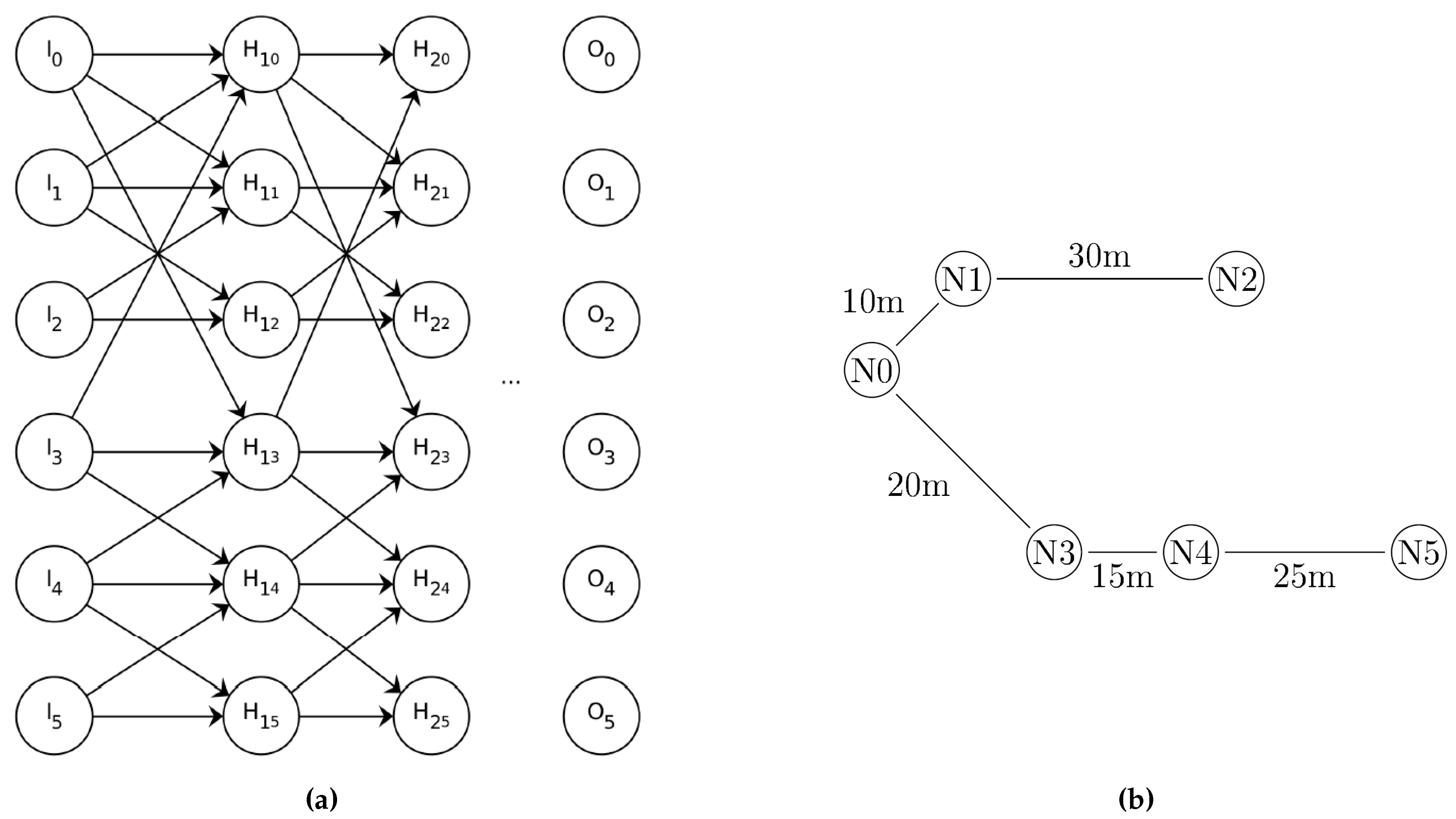
Figure 1a introduces a PANN implementation for the simple network depicted in
Figure 1b. The PM uses this concept to integrate the network’s structure especially in HF for higher order harmonics. Two case studies prove the strength of this method over conventional and other data-driven methods.
3.3. Related Subject Areas in Power Quality State Estimation
In electrical grids, SE is an approach to reduce costly measurements for extensive infrastructure. Especially for PQSE, a minimum of applied PQ meters is desirable, as these devices are very expensive.
[
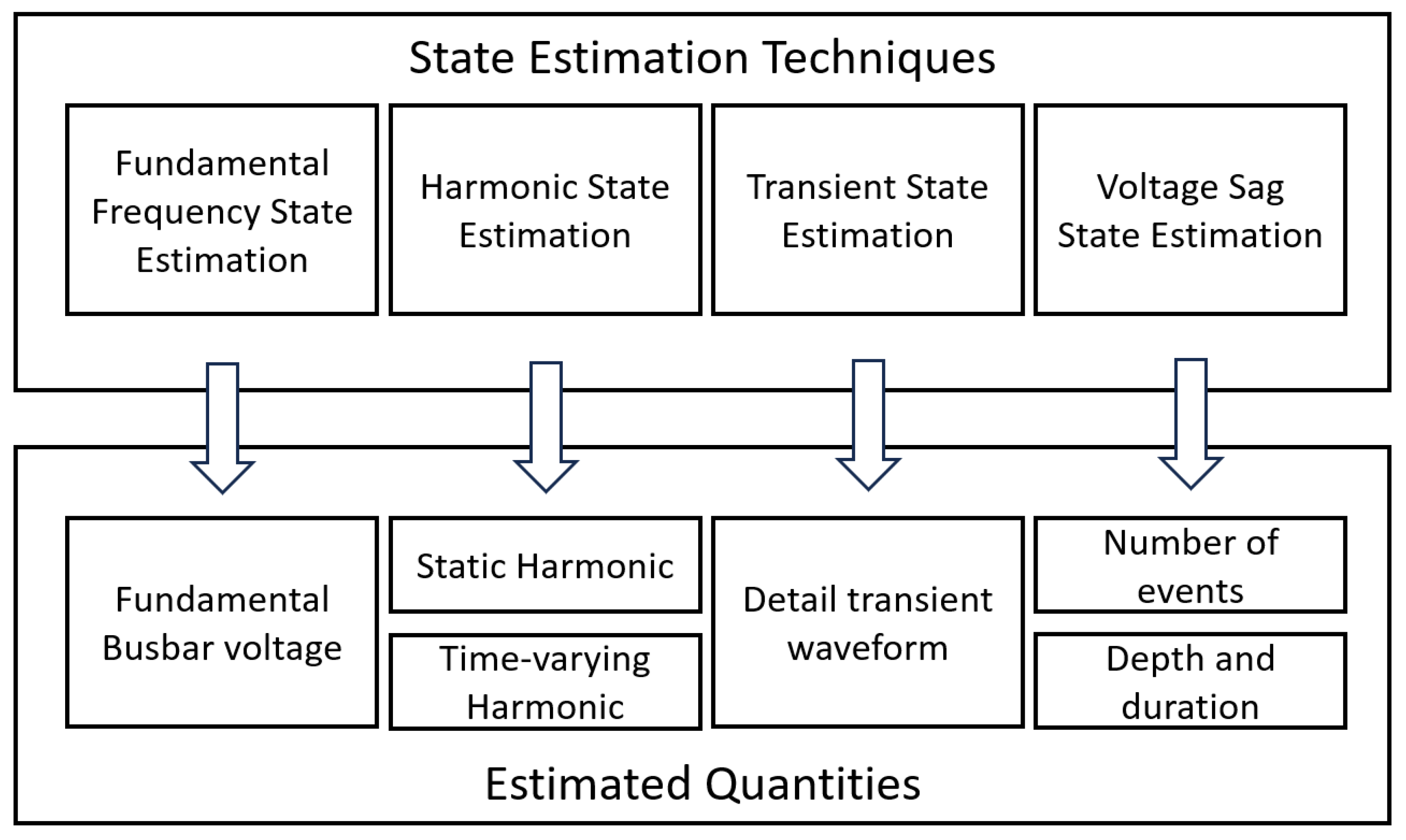
30] implemented and tested several methods for assessing PQ disturbances. The authors introduce a classification of error types to reduce the PQ phenomena to a limited set of algorithms. The presented article also employs this classification. Depending on the error type, the applied method varies. According to [
30], the classifications depicted in
Figure 2 consider the relevant criteria to assess PQ states.
Again, the applied methods are mainly WLS-based and may not be suitable for close-to-real-time applications. Fundamental frequency state estimation (FSE), voltage sag state estimation (VSSE), and HSE can be evaluated in the frequency domain. However, estimating transients in the time domain is a computationally costly process [
30]. The numerical integrator substitution for transient state estimation (TSE) requires a lot of time, as every time step of interest needs to be calculated [
31].
The presented work is embedded in a concept, which aims to combine TSE with FSE, and VSSE on the basis of the fast Fourier transform (FFT) and the presented HSE [
32]. Works like [
33,
34] analyze and simulate transient data within the frequency domain. This method will be used in sparse mode (sFFT) to also apply the presented HSE model to different time domain signals as shown in [
35].
3.4. Power Quality State Estimation Concept
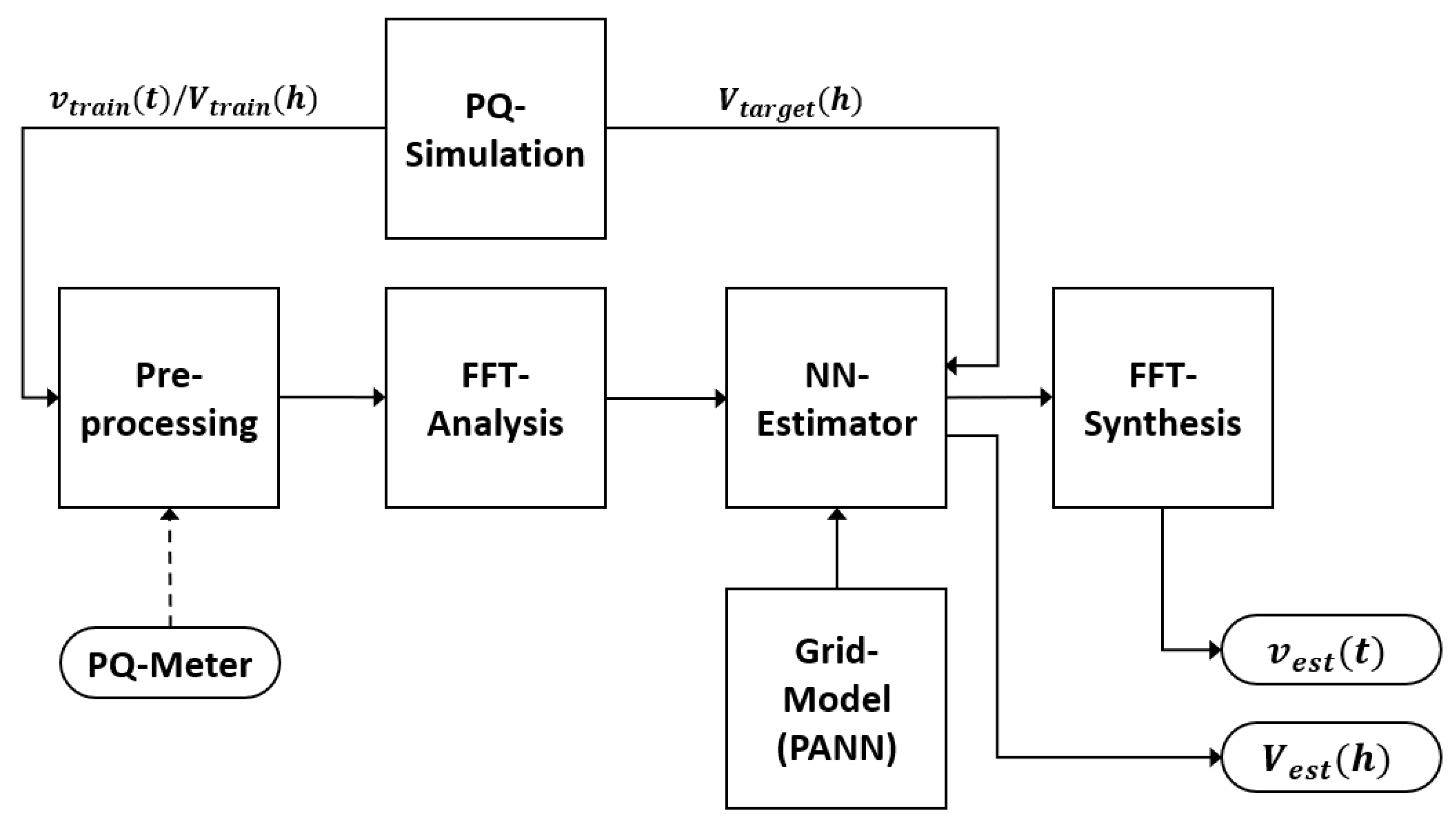
Summing up the literature review and the physical framework of this work, a state estimation concept is proposed, considering four main components:
Simulation environment for model training and validation
Optional preprocessing for transients (time span isolation) with FFT analysis and synthesis (not part of this work)
ANN estimator (few meters, close-to-real-time)
Integration of the grid model (network connections)
According to the described components, the correlating block diagram is depicted in
Figure 3. Training, validation, and testing of the model are solely done on simulation data.
This concept enables the evaluation of the fundamental frequency and harmonic components of the voltage signals as complex vectors. However, the Fourier transform yields complex coefficients for every frequency, which may not only include harmonics but also sub-harmonics, inter-harmonics, and supra-harmonics. The initial version of this estimator is only trained for a fixed range of 20 harmonics, omitting the FFT capabilities shown in
Figure 3. Therefore, the training dataset does not currently include any other data.
3.5. Case Study Setup and Simulation
For concept evaluation, a simulation environment was set up to generate PF, HF, and electro-magnetic transient (EMT) data. [
36] gives an extensive overview of EMT itself, waveforms, and simulation methods.
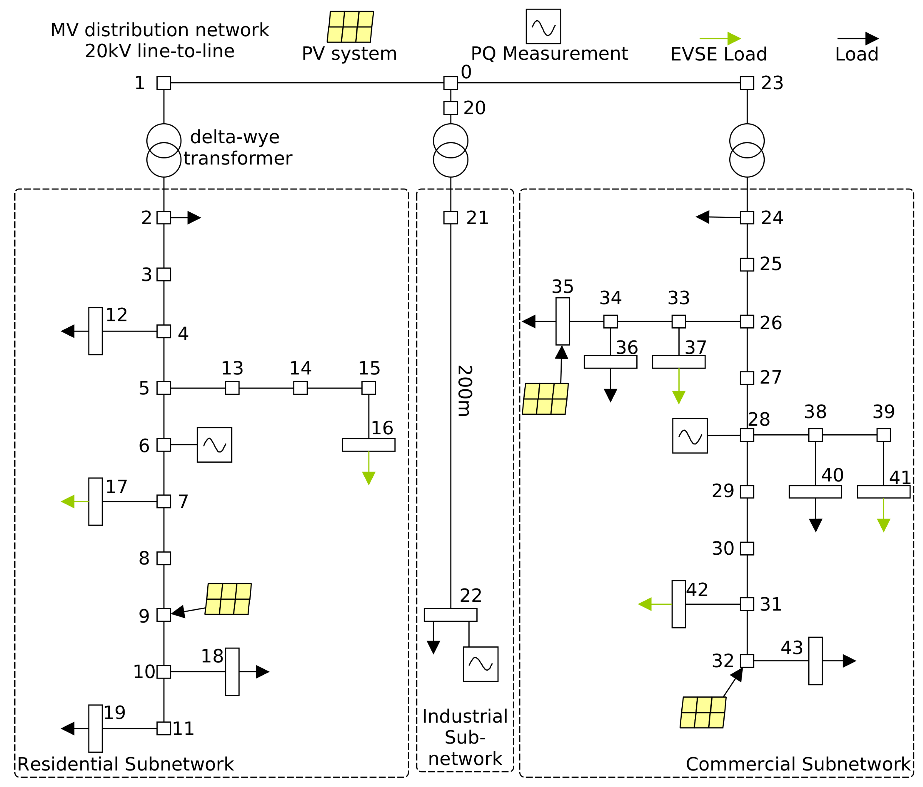
Figure 4 shows the simulated power grid, which was chosen to test the developed algorithms in depth due to its heterogeneous consumer structure (commercial, residential, industrial) and a typical rural distribution character of an LV/MV mixture. The IEEE33-bus test system from [
37] was also evaluated, but mainly for comparison with related work.
The OpenDSS simulation core was utilized to generate the training data for the reference grids. OpenDSS features various frequency-domain simulation modes like PF and HF [
38]. A Python application drives the OpenDSS kernel via the OpenDSSdirect.py library. This application controls the time series profile input, simulation commands, and data output for every simulated busbar. The HF results were used to train a fully connected DNN, a convolutional ANN (CNN), and a PANN model. These models calculate theoretic values for the bus voltages in the frequency domain.
Specific Extensions: The reference grid from [
39] is extended by 3 PV generators (bus 9:
, bus 32:
, bus 35:
), and 5 existing loads (busbars 16, 17, 37, 41, 42) are considered EVSE. Typical harmonic profiles realize harmonic current injection of these components. The other loads from [
39] are considered linear and behave as constant power drains.
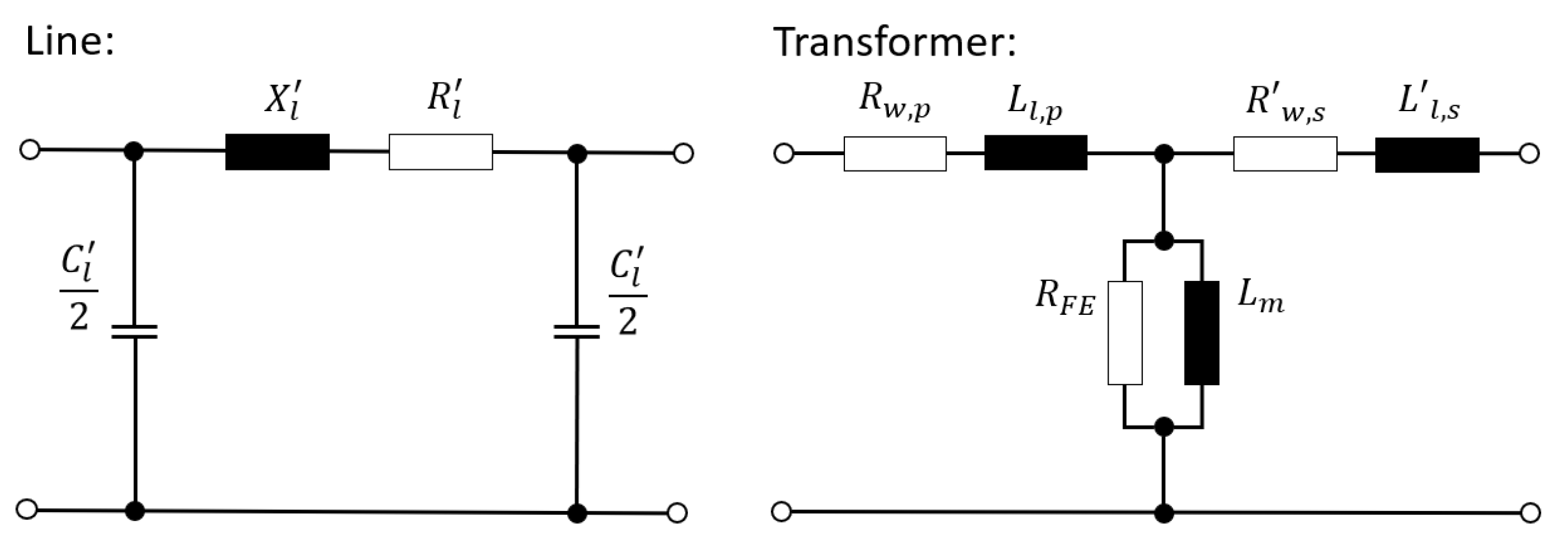
Figure 5 depicts the lumped circuit equivalents that OpenDSS uses internally for lines and transformers. As the simulations may include frequencies relevant for resonances, the lines’ capacitances need to be considered, too. Therefore,
Table 1 shows the full line parameters of the used types [
40]. To also create reasonable propagation of harmonics along MV cables, the MV busbar was split up, and the slack at busbar 0 is connected to the three transformers through 100-meter-long cables of type NA2XS2Y 1x95mm² each.
The transformers described in [
39] lack shunt components. In OpenDSS, the shunt components are considered relative dimensions.
is represented by the no-load losses
and
correspond to equation (
6).
Typical values for
and
can be found in [
41]. In this work for smaller substations (
),
and
are used.
PV-, EVSE-, and Load Profiles and Spectra: In total, a time span of a complete year in steps of one minute was simulated to generate training data. Every single load, EVSE, and PV system received an individual load profile. The specific matching of load profiles, PV profiles, spectra and references can be found in [
42]. In total, 525,600 simulated states are available for training, validation, and testing, but only 35,040 (15 minute steps) were used for this article.
3.6. Artificial Neural Network Architecture and Used Data
The used hyperparameters are depicted in
Table 2. The Adam optimizer is used due to its suitability for large datasets and multidimensional regression learning [
43]. As activation function leaky ReLU is used to reduce the risk of non-responsive neurons [
27].
Training, Validation and Testing: The training set consisted of 70% of the used data, 20% and 10% for validation and testing, respectively. As mentioned beforehand, the test set was generated with unknown load profiles and partially different harmonic spectra to observe the networks’ ability to generalize. These configurations can be found in [
42].
Input and Preprocessing: In addition to the significance of training ANNs on normalized input, the complex voltages of PQ-meters may be split into cartesian imaginary and real components. However, a special representation was tested and introduced to reduce the strong correlation between the imaginary and real components. Hence, the magnitude of the polar representation is used along with the imaginary part of
as input. Scaling is done by min/max normalization [
27].
Multi-Layer Perceptron Architectures: In the hidden layers, three architectures were tested. The input layer was set to a dimension of 3x2x20 (3 complex voltage phasor measurements at 20 harmonics) for all configurations. The connections to the hidden layers were set up in different ways.
Initially, tests were conducted with two dense layers with a flattened shape of 1x1760 neurons (expecting 44 nodes with complex bus voltages on the output layer at 20 harmonics). Architectures with more than two dense layers resulted in more trainable parameters. However, they yielded comparable or worse results. The second approach integrates the physical structure of the electrical grid into the connection scheme of the ANN, as explained above. Connections between the electrical network’s nodes are considered by the adjacency matrix. The network’s admittances are not considered.
For further comparison, a convolutional neural network (CNN) was implemented with similar hyperparameters. The convolutional layers start with a pointwise convolution (kernel: , stride: 1), then six depthwise convolutions (kernel: , stride: 1) are performed.
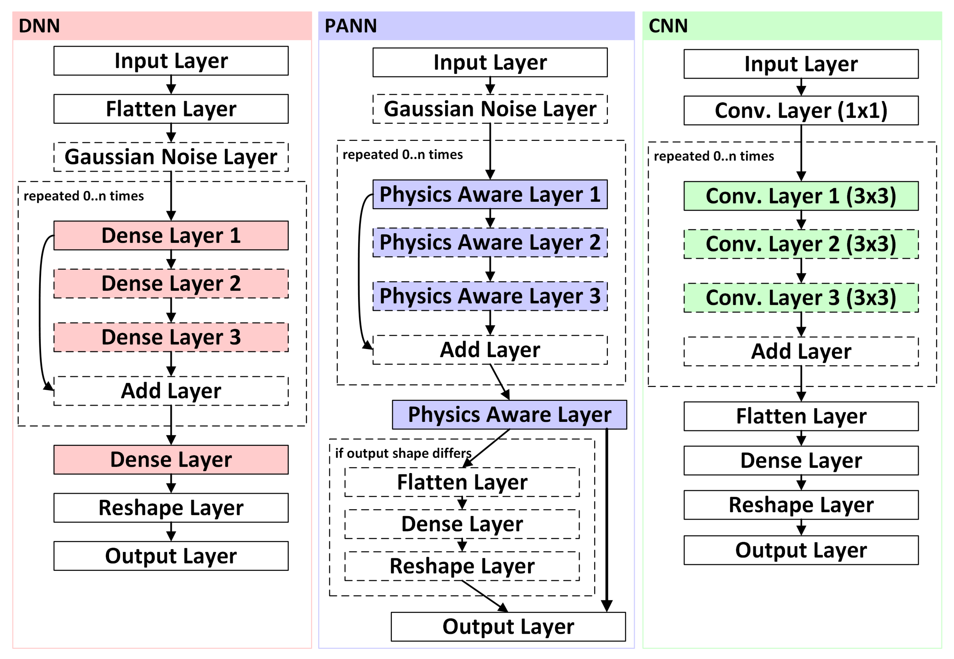
Figure 6 provides an overview of the PANN architecture compared to the simpler DNN and a CNN. The recursive equations (
7)-(
9) describe the mathematical framework for the PANN without reshaping layers.
Index
p marks the
n pruned adjacency layers, while
G notes a Gaussian layer, which is only active during training. It adds noise (
) to the input
X. The weight matrices in the adjacency layers
prune connections by setting weights to zero. This iterative description represents the path from a complex input matrix
X to the estimated matrix
.
Output-Data: All networks have output dimensions of 44x2x20 (44 estimated complex nodal voltages at 20 harmonics). The activation function in the output layer is a linear function.
4. Results
The overall results show the best accuracy for the PANN solution. However, the complexity of setting up the model is significantly higher than using DNN topologies.
4.1. Overall Results on Test Data
The mean squared error (MSE) is used as the loss function during the training process and as an important benchmark. It is defined as follows:
The definition describes the average over
n samples of the squared deviation of the estimate
from a target value
[
44]. Another method that is used to provide insight into the presented model’s precision is the mean absolute error (MAE). According to [
45], the MAE is the most natural measure, and within this work, it gives a better physical interpretation. The MAE can be described as depicted below in (
11).
In [
12] the normalized root MSE (NRMSE) was used for benchmarking and is defined as the root of the MSE over the datasets’ mean
[
46].
The NRMSE will be used for comparison with related work from [
12].
Additionally, the mean relative error (MRE) can be used to evaluate an estimator. [
47] used the MRE as the metric for the presented HSE. Actually, the article mentions the MSE, but in correspondence with the authors [
47], the following equation was provided:
Table 3 compares the final trained MSE loss of the tested networks. When the PANN is trained for more epochs, it significantly improves its accuracy, while the compared DNN only marginally improves. Generally, the compared CNN exhibits a higher validation loss within the conducted training. The MSE for 1,400 and 3,000 epochs is still higher than for the loss of the compared architectures.
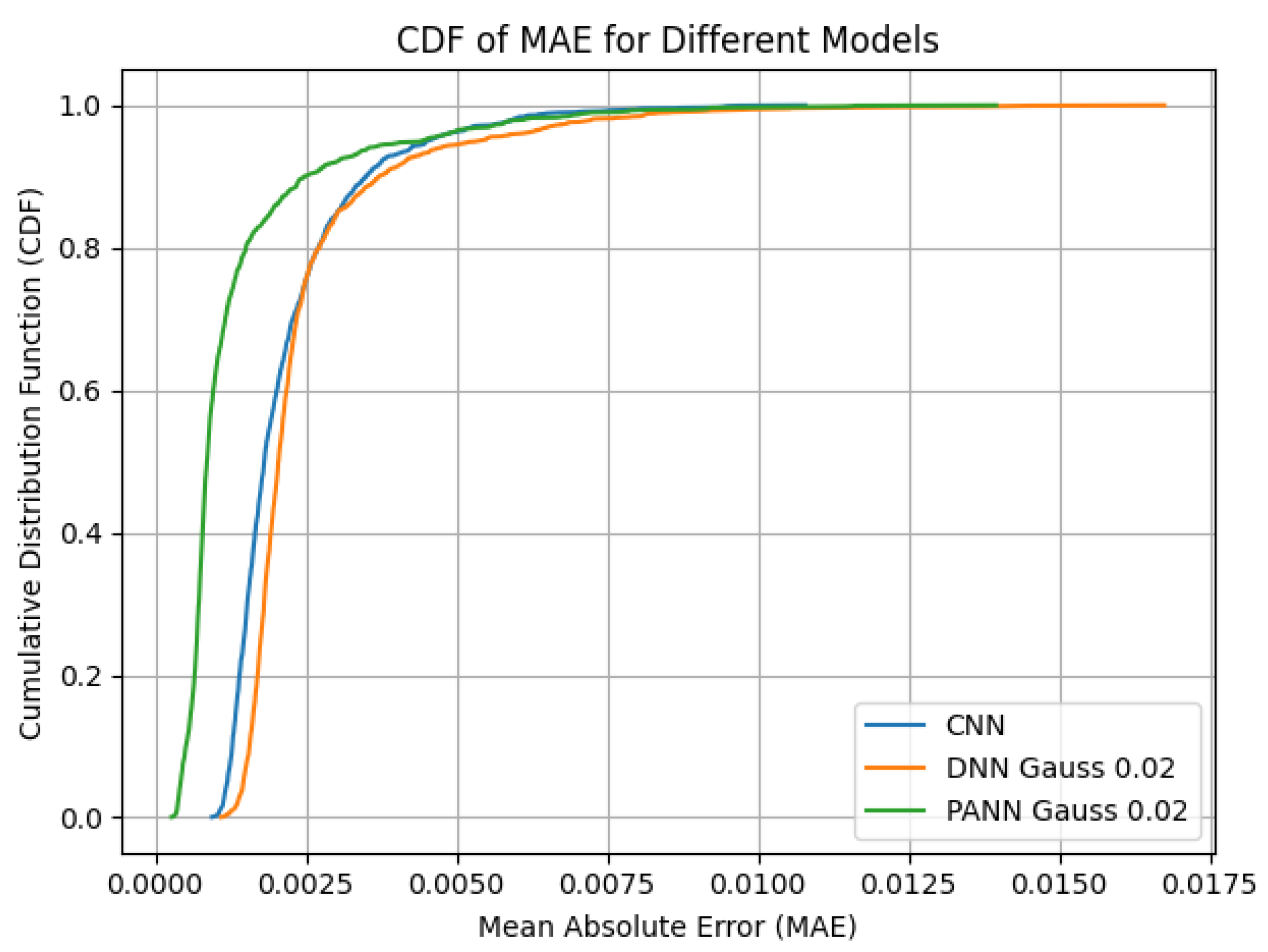
Figure 7 emphasizes the accuracy of the PANN architecture over the entire validation data set. A high curve’s steepness correlates with little error over the majority of the test dataset. The PANN shows a better overall performance and only few larger errors. In order to observe the THD,
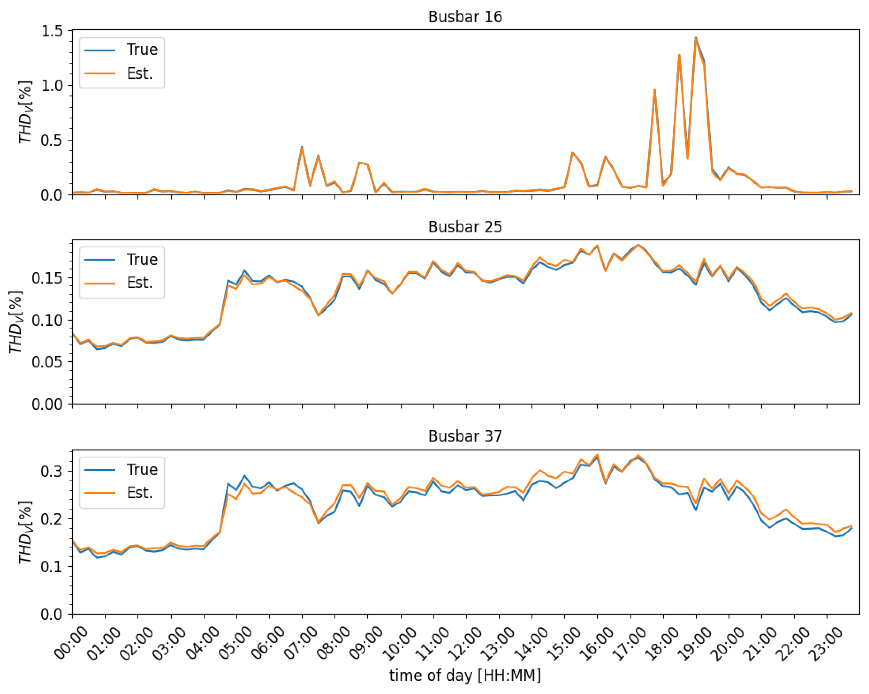
Figure 8 gives an impression of the voltage THD (
) for some busbars during a day in the test data set. One can see that while predictions for buses 16 and 25 show a good approximation, bus 37 features an underestimation for higher THD levels. However, the trend of the curve is still followed by the estimator.
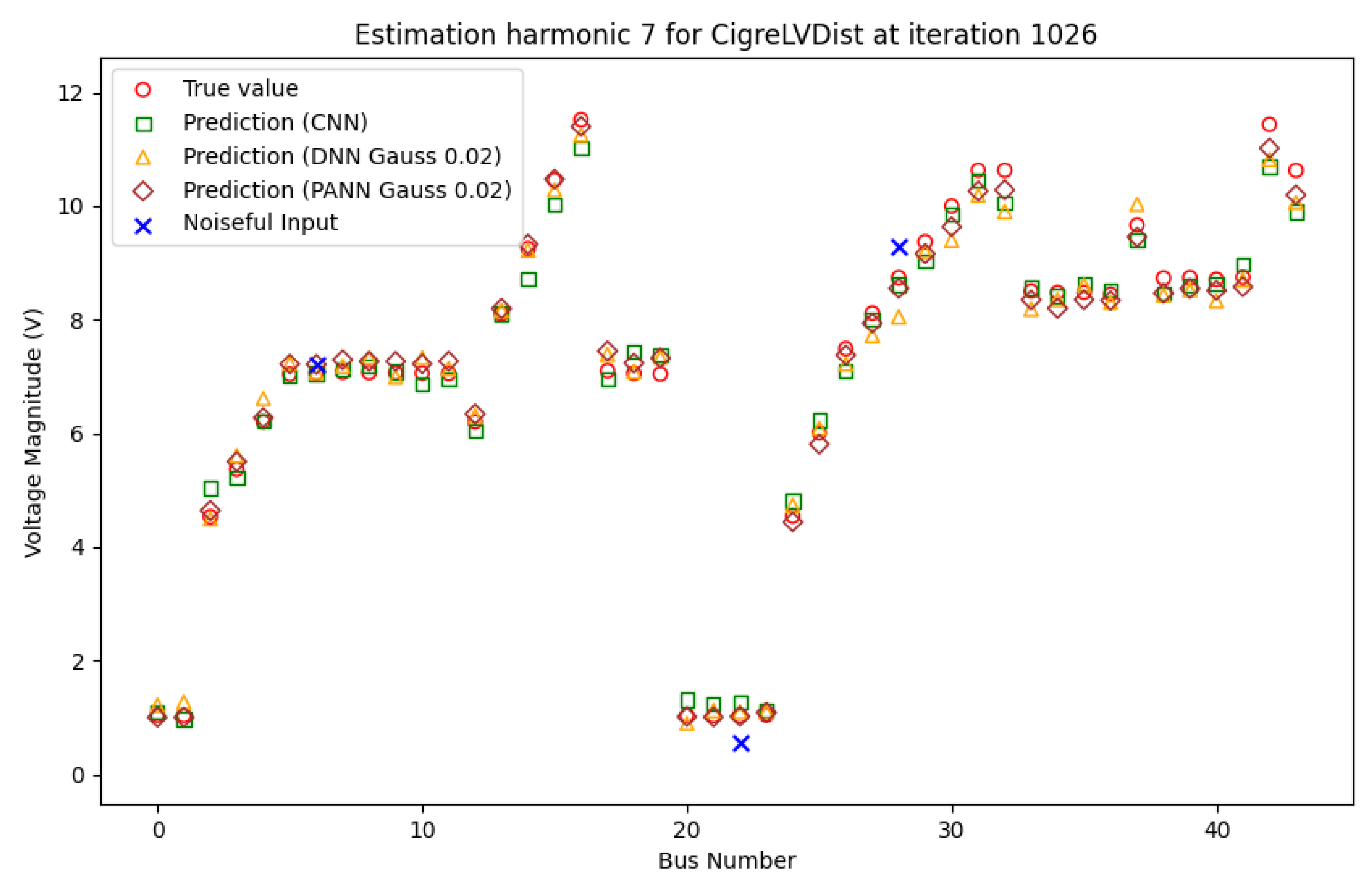
Figure 9 compares the simulated values, the DNN estimates, and the PANN estimates of one system state with regard to the 7
th harmonic order voltages. The precision of the PANN’s guesses is remarkable compared to the DNN’s and CNN’s. Even when there is a slightly disturbed measurement on bus 28, the network has a high ability to generalize. Additionally, on almost every bus, the DNN’s performance is worse than the PANN’s estimations.
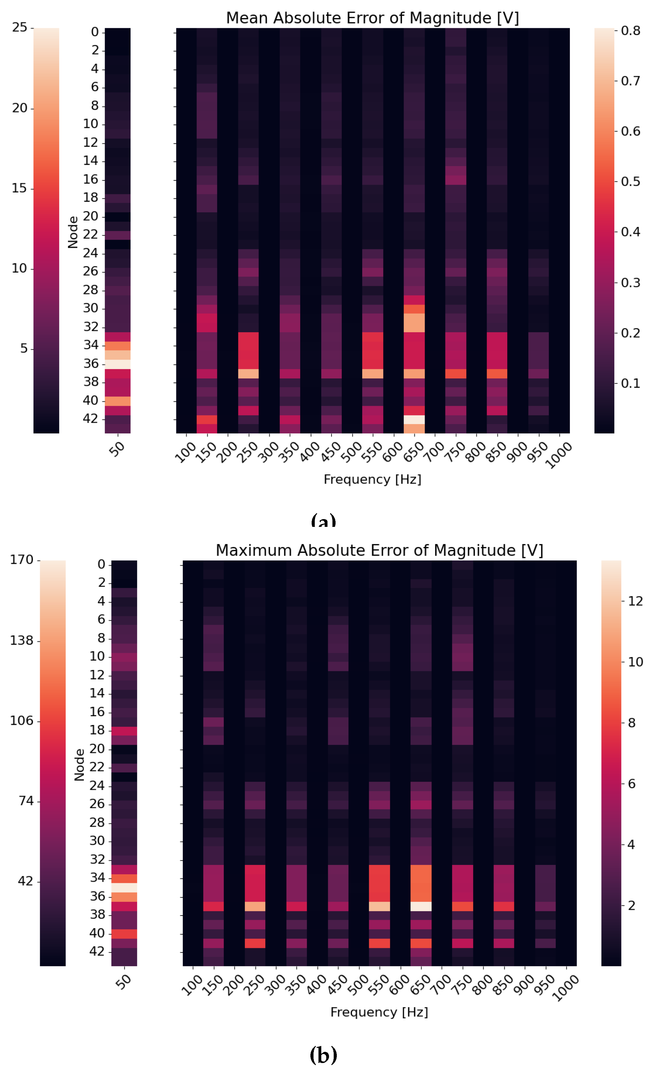
Looking at individual harmonics of the HSE, the heatmaps in
Figure 10 depict specific maximum MAE and maximum absolute errors over all nodes, as well as the measured harmonic frequencies. In detail, one can see that busbars 37 and 42 have the highest deviations among all harmonics. Busbars 35 and 36 have a high maximum absolute error and the highest MAE when it comes to estimating fundamental frequency values. That might be explained by the multiple branches within these sections. Especially around busbar 37, there is a EVSE, and a PV systems attached to these nodes. All harmonic currents will flow along these lines, influencing the harmonic level significantly as this subsystem exchanges high PF.
4.2. Comparison with Related Work
Focusing on HSE, different algorithms can be found in the current literature. This section evaluates and compares the most significant works according to the following criteria:
Estimated-Nodes-to-Meter-Ratio (ENMR)
Individual Precision/Quality of Estimations
Computational Performance/Execution Time
Estimated-Nodes-to-Meter-Ratio: To compare the amount of needed meter devices, the ENMR is introduced and defined as follows:
is the number of nodes in a network that are not measured and whose states will be estimated. The busbars, denoted by
, serve to collect measurement data.
Table 4 compares several works in the field of HSE for distribution grids. The ENMR shows that the PM is suitable for making good use of sparse measurement equipment. Only the study in [
20] achieves a similar but still smaller ratio. It is also noteworthy that the presented concept monitors harmonics up to the 20
th order, whereas works such as [
12] consider the 15
th order as the highest.
Individual Precision/Quality of Estimations: To achieve better comparability, the PM is also applied to the more common IEEE33-bus distribution system. The compared works [
12,
47] evaluate this feeder too. As the authors in [
47] also compared their work to the SVD method from [
13], these results are also listed. In order to emphasize the accuracy of certain harmonics,
Table 5 compares these metrics individually.
Especially for the HSE proposed in [
12], only four harmonic injections were considered, whereas our implementation of the feeder assumes five sources, like in [
47]. Three PQ meters are placed on buses 3, 13, and 29. Therefore, the ENMR is 10.
From the data given in [
12], the NRMSE was evaluated for each busbar individually. The maximum value of the individual busbar NRMSE results is compared in
Table 5. While the comparison of the NRMSE reveals better performance for estimation by the PANN at the fundamental frequency, the harmonic components are predicted similarly by the extended WLS method in [
12].
A different pattern occurs when comparing the MRE over the entire test data set with the techniques in [
47]. For harmonic orders 1, 3, and 7, the PANN provides better estimations than the compared methods. The MIQP and the WLS methods are able to predict the 5
th harmonic more accurately. Notably, the PANN’s fundamental frequency estimations exhibit very little MRE, while higher harmonics are in a similar range to the MIQP results. The significant difference in the 1
st harmonic may be explained by the MRE definition, our large test dataset, and just a few larger absolute errors, as explained above in
Figure 7.
Computational Performance/Execution Time: Especially when comparing the PM to conventional SE techniques like WLS, execution time is an important aspect for benchmarking. The presented study in [
12] compared execution times for WLS (
) with other methods from [
19,
20,
21] (all
) for estimations up to the 15
th order. In comparison, the PANN estimates the entire test dataset (3,504 harmonic states) within an inference time of
on an Intel® Core™ i7-12700K with a 25MB cache and a CUDA NVIDIA RTX A2000 graphics processor.
4.3. Influence of Noisy Measurement
To transfer this concept to real-world applications, the influence of noisy measurements was also considered. The authors in [
49] suggest error modeling by using Gaussian noise for PMU measurements. Authors of related work [
50] propose noise modeling with zero mean and
for voltage magnitude measurements in PF applications to increase the robustness of the model. To compensate similar effects, the models presented in this work can be trained with an optional Gaussian noise layer. The influence is presented in
Table 6. The validation loss MSE of different combinations is used as a marker over two test states. In the case of an ideal input value, the Gaussian layer will reduce the prediction’s accuracy slightly by 19.6% and 12.7%. However, when a noisy input is applied to the network, the precision of the predicted states is improved by 6.3% and 9.7%. This positive effect occurs because the ANNs have already learned to generalize during training on slightly altered data. This test is an indication to use the Gaussian layer as a possible improvement for application in real grids, where noisy measurement data is expected.
5. Discussion and Conclusion
We implemented a highly accurate HSE that focuses on harmonic and fundamental flows within a typical distribution grid topology. In direct comparison with DNN architecture, integrating the grid’s physical structure significantly reduces the validation loss of by 35.78%. The network’s short inference time of for estimating 3,504 system states demonstrates the potential for near-real-time applications.
Three measured nodes are sufficient to estimate 41 complex state variables per 20 harmonic frequencies in a highly branched distribution grid. The presented case study exhibits 3 substations, 2 voltage levels, 8 non-linear loads and generators, and 5 linear loads.
The latest literature does not present comparable precision at the given ratio of monitored locations to the number of states. Other articles, which have similar error rates on certain harmonics, use either more measuring devices (e.g., 6 PMUs on 33 buses [
47]) or require about 1 minute computational time for predictions [
12]. A second case study within the IEEE33-bus grid proves the gain in precision and the suitability of the used concept at higher voltage levels. These achievements highlight the use of PANN for PQSE in distribution grids.
The primary aim of our future work is to combine TSE, FSE, and HSE based on the presented HSE model. Next, the TSE will be implemented by adapting the ANN’s input to a dynamic structure that handles various spectral datasets. As a Gaussian layer already improved prediction of states based on noisy measurements, the PM will be tested in laboratory grids, too. Finally, another future task is the implementation of a controlling module, which ensures the accordance of estimated states to physical laws.
Author Contributions
Conceptualization, P.M. and M.d.K.; methodology, P.M, M.d.K. and P.L.; software, P.M and M.d.K.; validation, M.d.K. and P.M.; formal analysis, M.d.K. and P.M..; resources, M.d.K. and P.M.; data curation, M.d.K.; writing—original draft preparation, P.M.; writing—review and editing, X.X.; visualization, P.M. and M.d.K.; supervision, E.W. and I.S.; project administration, E.W., P.M., P.L.; funding acquisition, E.W. and I.S. All authors have read and agreed to the published version of the manuscript.
Funding
This research was funded by the German Federal Ministry for Economic Affairs and Climate Action grant number 03EI4048R.
Data Availability Statement
Conflicts of Interest
The authors declare no conflicts of interest. The funders had no role in the design of the study; in the collection, analyses, or interpretation of data; in the writing of the manuscript; or in the decision to publish the results.
References
- Schulz, D. Mains Disturbances - Theory, Simulation, Measurement and Evaluation: Per DIN VDE 0838, DIN VDE 0839 and the VDEW-Guidelines with Simulation-Examples in Simplorer and Measurements of grid-connected Photovoltaic Systems and Wind Power Generators (In German), 1. aufl. ed.; Vol. 115, VDE-Schriftenreihe Normen verständlich, VDE-Verl.: Berlin and Offenbach, 2004; p. 14.
- DIN Deutsches Institut für Normung e. V.. Voltage characteristics of electricity supplied by public electricity networks; German version EN 50160:2010 + Cor.:2010 + A1:2015 + A2:2019 + A3:2019, 2020.
- VDE. Electromagnetic compatibility (EMC) – Part 2-2: Environment – Compatibility levels for low-frequency conducted disturbances and signalling in public low-voltage power supply systems, 2020.
- Phadke, A.G.; Bi, T. Phasor measurement units, WAMS, and their applications in protection and control of power systems. Journal of Modern Power Systems and Clean Energy 2018, 6, 619–629. [Google Scholar] [CrossRef]
- Watson, N.R. Power quality state estimation. European Transactions on Electrical Power 2010, 20, 19–33. [Google Scholar] [CrossRef]
- Sanchez-Puentes, Y.; Argote-Parra, C.; Lakatt-Benavides, W.; Narvaez-Viana, J.; Nuñez-Alvarez, J.; Grimaldo-Guerrero, J. Influence of Photovoltaic Systems on Power Quality Problems. International Journal of Energy Economics and Policy 2023, 13, 185–190. [Google Scholar] [CrossRef]
- Ping, H.; Dong, L.; Xin, Q. Influence of Grid-connected Photovoltaic Systems on Power Quality. 2019 IEEE 2nd International Conference on Automation, Electronics and Electrical Engineering (AUTEEE) 2019.
- Gomez, J.C.; Morcos, M.M. Impact of EV battery chargers on the power quality of distribution systems. IEEE Transactions on Power Delivery 2003, 18, 975–981. [Google Scholar] [CrossRef]
- Bohn, J.K.; McMullen, D.W.; Save, P. Electric Vehicle Battery Charger Harmonics Study. Rosemead, CA, 1995.
- IEEE. 519-2022 - IEEE Standard for Harmonic Control in Electric Power Systems, 2022.
- Alliance for Telecommunications Industry Solutions. Federal Standard 1037C: Glossary of Telecommunications Terms. glossary.atis.org, accessed on 2024-05-13.
- Melo, I.D.; Pereira, J.L.; Variz, A.M.; Garcia, P.A. Harmonic state estimation for distribution networks using phasor measurement units. Electric Power Systems Research 2017, 147, 133–144. [Google Scholar] [CrossRef]
- Breda, J.F.; Vieira, J.C.M.; Oleskovicz, M. Three-phase harmonic state estimation for distribution systems by using the SVD technique. 2016 IEEE Power and Energy Society General Meeting (PESGM). IEEE, 2016, pp. 1–5.
- Bhujel, D.; Watson, N.R.; Jalal, T.S. Application of harmonic state estimation to a distribution system. 2017 IEEE Manchester PowerTech. IEEE, 2017, pp. 1–6.
- Zang, T.; Wang, Y.; Sun, H.; He, Z. Variable parameter Kalman filter based dynamic harmonic state estimation for power systems with wind energy integration. 2017 IEEE Conference on Energy Internet and Energy System Integration (EI2). IEEE, 2017, pp. 1–5.
- Lin, G. State Estimation in Medium Voltage Grids with incomplete measurement infrastructure (In German); Cuvillier Verlag: Göttingen, 2019; pp. 44, 57.
- Kelker, M.; Schulte, K.; Kroger, K.; Haubrock, J. Development and validation of a neural network for state estimation in the distribution grid based on uPMU data. 2019 Modern Electric Power Systems (MEPS). IEEE, 2019, pp. 1–6.
- Manitsas, E.; Singh, R.; Pal, B.C.; Strbac, G. Distribution System State Estimation Using an Artificial Neural Network Approach for Pseudo Measurement Modeling. IEEE Transactions on Power Systems 2012, 27, 1888–1896. [Google Scholar] [CrossRef]
- Bahabadi, H.B.; Mirzaei, A.; Moallem, M. Optimal Placement of Phasor Measurement Units for Harmonic State Estimation in Unbalanced Distribution System Using Genetic Algorithms. 2011 21st International Conference on Systems Engineering. IEEE, 2011, pp. 100–105.
- Arefi, A.; Haghifam, M.R.; Fathi, S.H. Distribution harmonic state estimation based on a modified PSO considering parameters uncertainty. 2011 IEEE Trondheim PowerTech. IEEE, 2011, pp. 1–7.
- Arefi, A.; Haghifam, M.R.; Fathi, S.H.; Niknam, T.; Olamaei, J. A novel algorithm based on Honey Bee Mating Optimization for distribution harmonic state estimation including distributed generators. 2009 IEEE Bucharest PowerTech. IEEE, 2009, pp. 1–7.
- Zhou, W.; Ardakanian, O.; Zhang, H.T.; Yuan, Y. Bayesian Learning-Based Harmonic State Estimation in Distribution Systems With Smart Meter and DPMU Data. IEEE Transactions on Smart Grid 2020, 11, 832–845. [Google Scholar] [CrossRef]
- Xie, Y.; Shao, Z.; Chen, F.; Lin, H. Harmonic State Estimation Based on Network Equivalence and Closed Loop GAN. 2023 8th Asia Conference on Power and Electrical Engineering (ACPEE). IEEE, 2023, pp. 1688–1693.
- Tran, M.Q.; Zamzam, A.S.; Nguyen, P.H.; Pemen, G. Multi-Area Distribution System State Estimation Using Decentralized Physics-Aware Neural Networks. Energies 2021, 14, 3025. [Google Scholar] [CrossRef]
- Zamzam, A.S.; Sidiropoulos, N.D. Physics-Aware Neural Networks for Distribution System State Estimation. IEEE Transactions on Power Systems 2020, 35, 4347–4356. [Google Scholar] [CrossRef]
- Schweppe, F.; Wildes, J. Power System Static-State Estimation, Part I: Exact Model. IEEE Transactions on Power Apparatus and Systems 1970, PAS-89, 120–125.
- Aggarwal, C.C. Neural Networks and Deep Learning: A Textbook, 2nd ed. 2023 ed.; Springer International Publishing and Imprint Springer: Cham, 2023; pp. 11,64,130–131.
- Haykin, S.S. Neural networks and learning machines,, 3rd. ed.; Pearson: New York, 2009; pp. 10–24. [Google Scholar]
- Fukushima, K. Visual Feature Extraction by a Multilayered Network of Analog Threshold Elements. IEEE Transactions on Systems Science and Cybernetics 1969, 5, 322–333. [Google Scholar] [CrossRef]
- Farzanehrafat, A.; Watson, N.R. Power Quality State Estimator for Smart Distribution Grids. IEEE Transactions on Power Systems 2013, 28, 2183–2191. [Google Scholar] [CrossRef]
- Marini, A.; Shabanzadeh, M.; Esmaeili, A. Chapter 8.2 - Power quality state estimation of power distribution systems: opportunities and challenges in observability enhancement. In Active Electrical Distribution Network: Issues, Solution Techniques, and Applications; Padmanaban, S.; Khan, B.; Mahela, O.P.; Alhelou, H.H.; Rajkumar, S., Eds.; Academic Press, 2022; pp. 243–284.
- Cooley, J.W.; Tukey, J.W. An algorithm for the machine calculation of complex Fourier series. Mathematics of computation 1965, 90, 297–301. [Google Scholar] [CrossRef]
- Ametani, A. The Application of the Fast Fourier Transform to Electrical Transient Phenomena. The International Journal of Electrical Engineering & Education 1973, 10, 277–287. [Google Scholar] [CrossRef]
- Tavighi, A.; Ahmadi, H.; Armstrong, M.; Martí, J.R. Discrete-Time Fourier Series to simulate transient over voltages in power systems. Electric Power Systems Research 2020, 188. [Google Scholar] [CrossRef]
- Li, B.; Jiang, Z.; Chen, J. On Performance of Sparse Fast Fourier Transform Algorithms Using the Flat Window Filter. IEEE Access 2020, 8, 79134–79146. [Google Scholar] [CrossRef]
- Mahseredjian, J.; Dinavahi, V.; Martinez, J.A. Simulation Tools for Electromagnetic Transients in Power Systems: Overview and Challenges. IEEE Transactions on Power Delivery 2009, 24, 1657–1669. [Google Scholar] [CrossRef]
- Baran, M.E.; Wu, F.F. Network reconfiguration in distribution systems for loss reduction and load balancing. IEEE Transactions on Power Delivery 1989, 4, 1401–1407. [Google Scholar] [CrossRef]
- Dugan, R.C.; Montenegro, D.; Ballanti, A. Reference Guide The Open Distribution Simulator (OpenDSS 9.0.0), 2020.
- CIGRE. Benchmark systems for network integration of renewable and distributed energy resources: Task force C6.04; Vol. 575, Brochures thématiques, CIGRE: Paris, 2014.
- Scheidler, A.; Thurner, L. pandapower v2.13.1. https://pandapower.readthedocs.io/en/v2.3.0/std_types/basic.html#lines, accessed on 2024-06-12.
- Oeding, D.; Oswald, B.R. Electrical Power Plants and Grids (In German); Springer Berlin Heidelberg: Berlin, Heidelberg, 2016; p. 229. [Google Scholar]
- de Koster, M.; Mack, P.; Lehnen, P. Code and Data Repository QUIRINUS Control, 2024.
- Kingma, D.P.; Ba, J. Adam: A Method for Stochastic Optimization, 2014.
- Sammut, C.; Webb, G.I., Eds. Encyclopedia of machine learning and data mining, second edition ed.; Springer Reference, Springer: New York, NY, 2017; p. 808.
- Willmott, C.J.; Matsuura, K. Advantages of the mean absolute error (MAE) over the root mean square error (RMSE) in assessing average model performance. Climate Research 2005, 30, 79–82. [Google Scholar] [CrossRef]
- Janssen, P.; Heuberger, P. Calibration of process-oriented models. Ecological Modelling 1995, 83, 55–66. [Google Scholar] [CrossRef]
- Ahmadi-Gorjayi, F.; Mohsenian-Rad, H. A Physics-Aware MIQP Approach to Harmonic State Estimation in Low-Observable Power Distribution Systems Using Harmonic Phasor Measurement Units. IEEE Transactions on Smart Grid 2023, 14, 2111–2124. [Google Scholar] [CrossRef]
- Wang, Y.; Ma, H.; Xiao, X.; Wang, Y.; Zhang, Y.; Wang, H. Harmonic State Estimation for Distribution Networks Based on Multi-Measurement Data. IEEE Transactions on Power Delivery 2023, 38, 2311–2325. [Google Scholar] [CrossRef]
- Brown, M.; Biswal, M.; Brahma, S.; Ranade, S.J.; Cao, H. Characterizing and quantifying noise in PMU data. 2016 IEEE Power and Energy Society General Meeting (PESGM). IEEE, 2016, pp. 1–5.
- Zhang, L.; Wang, G.; Giannakis, G.B. Real-Time Power System State Estimation and Forecasting via Deep Unrolled Neural Networks, 2019.
Figure 1.
In a PANN connections within the ANN correspond to physical connections from the electrical network. (a) Pruned ANN architecture. (b) Example of an electrical network with 6 nodes and 5 connecting lines.
Figure 1.
In a PANN connections within the ANN correspond to physical connections from the electrical network. (a) Pruned ANN architecture. (b) Example of an electrical network with 6 nodes and 5 connecting lines.
Figure 2.
Classification of power quality state estimation techniques according to [
30]. The four presented classifications cover the majority of PQ markers, or derivates of estimated quantities may be evaluated. E.g., a flicker can be calculated from fundamental frequency state estimation data.
Figure 2.
Classification of power quality state estimation techniques according to [
30]. The four presented classifications cover the majority of PQ markers, or derivates of estimated quantities may be evaluated. E.g., a flicker can be calculated from fundamental frequency state estimation data.
Figure 3.
The suggested idea uses data from either simulation or PQ meters (dashed line). The simulation environment provides data in the frequency and time domain. Depending on the chosen input, FFT algorithms are employed. Outputs of the SE are either detailed voltage waveforms or complex busbar voltages of harmonics h.
Figure 4.
The heterogeneous distribution network for simulation and verification of harmonic state estimation concept [
39]. We modified the original network to feature better harmonic characteristics. Three PQ meters are placed for estimation.
Figure 4.
The heterogeneous distribution network for simulation and verification of harmonic state estimation concept [
39]. We modified the original network to feature better harmonic characteristics. Three PQ meters are placed for estimation.
Figure 5.
Circuit equivalents showing the considered components in the OpenDSS simulation. On the left, the typical -equivalent for lines is depicted. On the right, a transformer with leakage inductances /, winding resistors /, main reactance , and iron resistor is shown.
Figure 5.
Circuit equivalents showing the considered components in the OpenDSS simulation. On the left, the typical -equivalent for lines is depicted. On the right, a transformer with leakage inductances /, winding resistors /, main reactance , and iron resistor is shown.
Figure 6.
General overview of the compared architectures and layers used. The developed framework allows an individual number of layers. The DNN and the PANN models optionally use an additional noise layer on the input data. In this article, 2 dense layers, 7 convolutional, and 6 physics-aware layers were used.
Figure 7.
Comparison of cumulative distribution functions of the mean absolute errors within the test dataset for CNN, DNN and PANN architectures.
Figure 7.
Comparison of cumulative distribution functions of the mean absolute errors within the test dataset for CNN, DNN and PANN architectures.
Figure 8.
Example prediction of the PANN model over 24 hours for example buses across the reference grid. Harmonic orders from 2 to 20 were considered.
Figure 8.
Example prediction of the PANN model over 24 hours for example buses across the reference grid. Harmonic orders from 2 to 20 were considered.
Figure 9.
Example for an estimated state on 7th harmonic order. Voltages over all nodes are referenced to 20kV level. Red circles represent the simulation data, blue crosses mark the placed meter position. The PANN is able to predict the busbar voltages very accurately.
Figure 9.
Example for an estimated state on 7th harmonic order. Voltages over all nodes are referenced to 20kV level. Red circles represent the simulation data, blue crosses mark the placed meter position. The PANN is able to predict the busbar voltages very accurately.
Figure 10.
Errors in magnitudes for the physics-aware model after reverting normalization with respect to 20kV as a reference. (a) Mean absolute error fundamental (left scale) and harmonics (right scale). (b) Maximum absolute error fundamental (left scale) and harmonics (right scale).
Figure 10.
Errors in magnitudes for the physics-aware model after reverting normalization with respect to 20kV as a reference. (a) Mean absolute error fundamental (left scale) and harmonics (right scale). (b) Maximum absolute error fundamental (left scale) and harmonics (right scale).
Table 1.
Line parameters used for the grid from [
39] to model frequency dependencies accurately.
Table 1.
Line parameters used for the grid from [
39] to model frequency dependencies accurately.
| Line types |
|
|
|
| UG1 |
0.162 |
0.0832 |
210.0 |
| UG2 |
0.2647 |
0.0823 |
210.0 |
| UG3 |
0.822 |
0.0847 |
210.0 |
| OH1 |
0.4917 |
0.2847 |
10.0 |
| OH2 |
1.3207 |
0.321 |
10.0 |
| OH3 |
2.0167 |
0.3343 |
10.0 |
| NA2XS2Y 1x95 12/20kV |
0.313 |
0.132 |
216.0 |
Table 2.
Overview of the most important hyperparameters for implemented DNN, CNN and PANN.
Table 2.
Overview of the most important hyperparameters for implemented DNN, CNN and PANN.
| Parameter |
DNN |
PANN |
CNN |
| Batch-size |
16,384 |
16,384 |
16,384 |
| No. of hidden layers |
2 |
6 |
7 |
| Loss function |
MSE |
MSE |
MSE |
| Activation |
Leaky ReLU |
Leaky ReLU |
ReLU |
| Optimizer |
Adam |
Adam |
Adam |
| Skip Connections |
Yes |
Yes |
No |
Table 3.
Overall network minimum MSE validation loss of all trained models over different amounts of epochs.
Table 3.
Overall network minimum MSE validation loss of all trained models over different amounts of epochs.
| Epochs |
DNN |
CNN |
PANN |
| 1400 |
|
|
|
| 3000 |
|
|
|
Table 4.
Comparison of related work regarding grid complexity, ENMR, and estimated harmonic orders. Technique abbreviations: Modified Particle Swarm Optimization (MPSO), Sparse Bayesian Learning (SBL), Mixed-Integer Quadratic Programming (MIQP).
Table 4.
Comparison of related work regarding grid complexity, ENMR, and estimated harmonic orders. Technique abbreviations: Modified Particle Swarm Optimization (MPSO), Sparse Bayesian Learning (SBL), Mixed-Integer Quadratic Programming (MIQP).
| Ref. |
Year |
Method |
Case study grid |
ENMR |
Harm. ord. |
| [13] |
2016 |
SVD |
IEEE13-bus |
1.6 |
11 |
| [20] |
2011 |
MPSO |
Radial 70-bus |
10.67 |
13 |
| [15] |
2017 |
KF |
IEEE13-bus |
n.a. |
n.a. |
| [22] |
2020 |
SBL |
IEEE13-bus |
1.2 |
13 |
| [14] |
2017 |
SVD |
Real 21-bus |
2.0 |
13 |
| [12] |
2017 |
WLS |
Indiv. 33-bus |
3.13 |
15 |
| [47] |
2023 |
MIQP |
IEEE33-bus |
4.5 |
7 |
| [48] |
2023 |
Var. |
IEEE33-bus |
2.67 |
7 |
| [23] |
2023 |
GAN |
IEEE33-bus |
4.5 |
n.a. |
| PM |
2024 |
PANN |
CIGRE LV |
13.67 |
20 |
| PM |
2024 |
PANN |
IEEE33-bus |
10.0 |
20 |
Table 5.
Comparison of related work and proposed method on the IEEE33-bus grid across all estimated nodal voltage phasors.
Table 5.
Comparison of related work and proposed method on the IEEE33-bus grid across all estimated nodal voltage phasors.
| Metric |
Maximum NRMSE |
MRE |
| Harm. ord. |
PANN |
WLS[12] |
PANN |
MIQP[47] |
SVD[47] |
| 1st
|
0.0023 |
0.0079 |
0.0009 |
25.226 |
2,007.9 |
| 3rd
|
0.0847 |
0.0991 |
0.04628 |
0.0718 |
101 |
| 5th
|
0.1948 |
0.0905 |
0.1163 |
0.0917 |
141 |
| 7th
|
0.0592 |
0.0905 |
0.0388 |
0.1590 |
202 |
Table 6.
Minimum MSE loss on the validation set with and without input noise () and Gaussian layer with in two trial runs of PANN models trained over 3000 epochs.
Table 6.
Minimum MSE loss on the validation set with and without input noise () and Gaussian layer with in two trial runs of PANN models trained over 3000 epochs.
| |
Ideal Input |
Noisy Input |
| Trial |
- |
Gauss. Lay. |
- |
Gauss. Lay. |
| 1 |
|
|
|
|
| 2 |
|
|
|
|
|
Disclaimer/Publisher’s Note: The statements, opinions and data contained in all publications are solely those of the individual author(s) and contributor(s) and not of MDPI and/or the editor(s). MDPI and/or the editor(s) disclaim responsibility for any injury to people or property resulting from any ideas, methods, instructions or products referred to in the content. |
© 2024 by the authors. Licensee MDPI, Basel, Switzerland. This article is an open access article distributed under the terms and conditions of the Creative Commons Attribution (CC BY) license (http://creativecommons.org/licenses/by/4.0/).
