Predicting Surface Roughness and Grinding Forces in UNS S34700 Steel Grinding: A Machine Learning and Genetic Algorithm Approach to Coolant Effects

In the realm of digitalization, data play a crucial role across various scientific fields, from physics to engineering. Analyzing data with advanced technologies like artificial intelligence enhances en-gineers' ability to make informed judgments on product quality. This study aligns with the digital-ization trend by implementing formula generation, generalization, and optimization using genetic algorithms and three machine learning approaches: support vector regression, Gaussian process regression, and artificial neural networks, on a grinding process dataset from a previous study on UNS S34700 steel. The study introduces new approaches by considering three different grinding wheels and four cooling and lubrication solutions as influential process parameters, previously considered qualitative and fixed in earlier literature. Additionally, seven different depths of cut were implemented to measure surface roughness and grinding forces (tangential and normal). Qualitative data were encoded into quantitative data using standard techniques. By enhancing genetic algorithm optimization, a relational formula with 25 coefficients was developed to describe the relationship between input parameters and outputs. Three machine learning algorithms were evaluated for predicting the relationship between predictors and responses. The flexibility and scalability of these methods, combined with the relational formula, provide a sophisticated ap-proach for future expansions. The formula evaluation achieved around 85% accuracy for surface roughness and 90% for grinding forces. In machine learning approaches, the GPR method reached model stability with an R² of around 0.98 and a mean accuracy of 93%, while the ANN reached an R² of around 0.96 and a mean accuracy of 90%. This shows that machine learning approaches are more suitable than formula generalization. The scalability and flexibility of machine learning help generalize with more data variety, while the formula evaluation only accepted current data sets. Furthermore, ML methods achieve high accuracy and are suitable for predicting future data, aligning with digitalization and trend prediction.

Keywords:

Subject: Engineering - Mechanical Engineering

1. Introduction

Austenitic stainless steels (ASSs) are widely known to exist in stable states depending on their chemical and mechanical conditions [1,2]. UNS S34700 steel, a metastable austenitic stainless steel, is widely utilized in the food, chemical, petrochemical, and medical industries [3]. Because austenitic stainless steels like type AISI 347 have good resistance to sensitisation and creep deformation, they are commonly used in components designed for high-temperature applications such as nuclear reactors, boilers, superheaters, and chemical reactors [4]. One of the most important criteria in these areas is fine surface finish, which AISI 347 steels can achieve through the grinding process. The ultimate surface quality of a processed workpiece significantly influences strength, friction, heat generation, wear, and fatigue resistance. Therefore, the specified grade of surface finish is usually indicated based on its applicability [5,6].

Grinding turns out to be the most practical and cost-efficient machining operation when it comes to achieving a fine high-quality surface. As the most common precision machining technique in the industry, it is important to monitor the efficiency of grinding operations. The choice of parameters, such as wheel speed, table speed, cross feed, depth of cut, dressing depth, coolant supply has a significant impact on the efficiency of the grinding process [7,8,9].

Machining factors such as surface roughness and cutting force directly impact the surface quality of workpieces. Additionally, forecasting these parameters is facilitated by models constructed in previous publications [10,11,12]. Agarwal et al. [13] studied the effects of different cutting parameters on surface finish such as material removal rate (MRR), surface roughness and surface burn. The results revealed that table speed, depth of cut, grit size, and abrasive grain density are the most important elements influencing the surface integrity using a silicon carbide grinding wheel. A decrease in depth of cut and table speed also results in less subsurface damage and surface roughness.

Machine learning (ML) techniques are used to forecast ideal machining parameters and fault detection as a predictive maintenance solution. ML approaches are highly beneficial in enhancing the prediction of grinding factors including cutting forces, tool wear, tool life [14], remaining useful life prediction, wheel wear detection [15], surface roughness prediction, grinding burn, estimation of grinding specific energy [16], wheel loading, and crack detection [17]. Because of its capability to identify extremely sophisticated and nonlinear patterns in data, the data-driven approach based on machine learning is the researcher’s main focus [18].

Gopan et al. [6] tried to use a hybrid ANN-PSO strategy to multi-objective optimize the surface grinding process on AISI D2 steel. Table speed, cross feed, and depth of cut were the machining parameters chosen for optimization, with the goals of minimizing surface roughness, F_Y, and F_X.

The confirmatory experiments for the ANN-PSO approach yielded error percentages of 9.8% for surface roughness, 3.75% for F_X, and 1.35% for F_Y. For multi-objective optimization in complex and nonlinear scenarios, the ANN-PSO method outperforms the traditional RSM-MOGA method.

Kant et al [19] developed an artificial neural network model to estimate the cutting energy of carbon steel during grinding based on data from 27 trials by adjusting process parameters (spindle speed, depth, width of cut, and feed rate). The cutting energy was predicted by the model used with a 98.5% accuracy rate.

The experimental data collected over five processes and optimization approaches employing neural model-based control strategies for the industrial grinding process were reported in the study by [20]. Another result of the study was optimizing a techniques affecting machining of steel-based tools through the use of neural networks.

Prashanth et al. [10] used machine learning to estimate the grinding variables for Inconel 751 under various environmental conditions. The aim of their study was to use machine learning methods to link the input and output characteristics of grinding Inconel 751. The methods for predicting the variables during Inconel 751 grinding were three different types of ML algorithms: support vector machine (SVM), boosted tree ensemble approaches, and Gaussian process regression (GPR). The GPR predicted grinding forces and temperature with relatively better R² score and RMSE value at wheel work contact. It is clear that the GPR Matern 5/2 model produces an accurate forecast, especially when predicting F_t, with constant R² values ranging from 0.85 to 0.9.

In order to predict the material removal rate for Inconel-718, Zhang et al. [21] used the electrical discharge diamond grinding (EDDG) and developed the GPR model whose input variables were wheel speed, current, pulse-on-time, and duty factors. The performance of the model was shown accurate and stable. In particular, the GPR model reaches the correlation coefficient (CC), mean percentage error (MPE), root mean square error (RMSE), and mean absolute error (MAE) of 99.17%, −0.55%, 0.6787, and 0.3789, respectively.

Prabhu et al [22] attempted to disperse multiwall carbon nanotubes (MWCNT) into cutting fluids of SAE 20W40 oil. Using L8 orthogonal Taguchi design of experimental procedures in CNC grinding, AISI D3 Tool steel was ground. CNC grinding was applied to AISI D3 Tool steel using L8 orthogonal Taguchi design of experimental methodologies. The experimental data were trained with the feedforward ANN method using Levenberg–Marquardt algorithm and the significant variables were identified. With the ANN model, the maximum test errors for surface roughness are 10.31% and 11.3% for the cases with and without carbon nanotubes.

A unique method for predicting the surface roughness of the Al-based MMC in cylindrical grinding was presented by Ucar et al. [23] and it has been effectively implemented. An optimized GPR model was created using a real-life dataset collected experimentally, from the other research. The suggested machine learning-based GPR model proved to be a promising way to enhance machining quality of the Al MMC materials when analysing the surface roughness.

Finding methods to establish the relationship between the input parameters obtained from experimental processes and output variables has been challenging research for engineers and authors in this field until now. Researchers also continue to conduct a techniques to predict output variables accurately through efficient quantitative models [24,25,26].

K.A. Abou-El-Hossein et al [27] published a paper about optimizing cutting force parameters using response surface method on modified AISI P20 tool steel during end-milling process. Predictive models were developed for cutting conditions including feed rate, cutting speed, grinding depth of cut, and radial depth of cut. Based on variance analysis, the most effective input parameters and the interactions of parameters were calculated. The parameters in this research were optimized and results were predicted with a 95% confidence interval.

Noordin et al. [27] used a model to establish a relationship between parameters to predict the tangential cutting force in turning of AISI 1045. They concluded that feed rate and side cutting edge angle are the main factors affecting the output variable.

The artificial neural network (ANN) has been used in many publications as one of the most accurate prediction methods in recent years. The versatility of ANN is due to its ability to handle non-linear systems, particularly in those systems where their definition is dynamic by various levels of a large number of parameters. The capability of ANN methods mostly comes from their versatility to train from past data and predict based on errors. The ANN can monitor surface roughness and grinding forces in industrial grinding processes for prediction, preventing faults subsequent data in process [28].

The authors [28] proposed dynamic models for the case of turning of AISI 4140 steel. They developed their study using ANN and support vector regression (SVR) methods in order to predict the cutting force and surface roughness. The results were validated and confirmed the accuracy of these techniques. The performance of the methods showed a fairly high detection accuracy in this research.

Gupta [29] conducted a study to predict surface roughness based on cutting speed, feed rate and cutting time. The methods that were used to calculate surface roughness from outputs factors were response surface methodology, ANN, and support vector regression (SVR). The results showed that the ANN and SVR models achieved higher accuracy than the response surface methodology model. The ANN model achieved an MAE of 0.0631 and an RMSE of 0.0501. In comparison, the SVR model recorded an MAE of 0.0898 and an RMSE of 0.0795. The R² was 0.9013 for ANN and 0.9273 for SVR. Table 1 depicts a comprehensive assessment of available research in the industrial grinding and machining process that uses artificial neural networks as a ground truth approach to anticipate and determine a relationship between input parameters.

The literature review clearly shows that many studies consider a wide range of grinding parameters. However, implementing all parameters is not always cost-optimized, and some grinding processes do not require specific parameters. Notably, only one study considered coolant as a changing parameter, while other studies fixed it, usually on MQL. None of the studies considered different grinding wheels, which are typically set to one model. The effects of different coolants and grinding wheels remain largely unexplored.

Previous studies [31,32] included a grinding test dataset with three different grinding wheels, four different coolants, and seven depths of cut. This approach is promising for considering these two often overlooked parameters in assessing surface roughness quality. Most studies enhance their models using ANN algorithms as the main method, with some also employing Support Vector Machines (SVM). These two methods are well-known and widely adopted due to their stability, as reported in the literature.

2. Materials and Methods

2.1. Experimental Setup

The experimental data were sourced from previous studies [31,32]. Surface grinding tests were conducted on hardened stainless steel (UNS S34700) using a 20-mm width M7135ANANTONG SHUANGZANG-NC surface grinding machine in down-grinding (plunge) mode. Several parameters were varied during the experiments to evaluate their effects on surface roughness and grinding force, while the remaining parameters were kept constant. Table 2 provides details of the experimental setup and the constant parameters used in the current grinding trials.

The study examined how changes in grinding input parameters affect output conditions. Surface roughness and grinding forces (tangential and normal) were measured using seven different depths of cut, three types of grinding wheels, and four cooling methods. The type of coolant and grinding wheel, which are qualitative factors, along with the depth of cut, a quantitative factor, directly impact surface roughness and grinding forces. Details of these variable parameters and their levels are provided in Table 3.

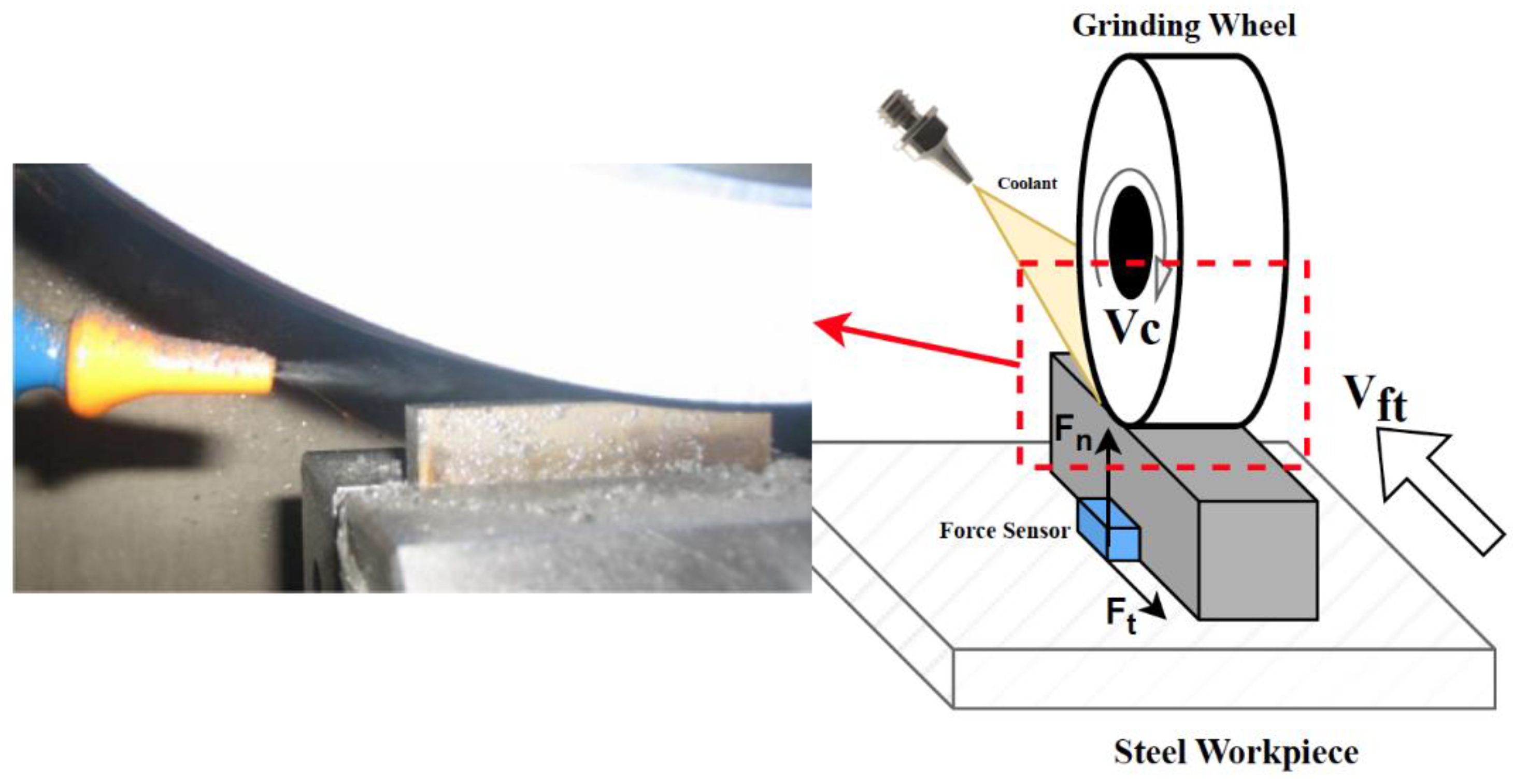
After the tenth pass, surface roughness and grinding forces were measured. In accordance with DIN EN ISO 3274:1998, the workpiece roughness was assessed using a mobile roughness measurement tool (DIAVITE AG) with a cut-off length of 0.8 mm. Surface roughness (R_z) across the grinding direction was measured at five different locations on the ground surface at the end of each test. A four-component dynamometer (Kistler type 9272) was used to measure the grinding force components while the workpiece was clamped with specific equipment (see Figure 1).

2.2. Dataset Evaluation

In a typical grinding process, numerous factors come into play. However, assessing all these variables at different levels necessitates a complex testing procedure, leading to costly and often impractical results in each trial. Considering the main factors that influence grinding quality and the machine’s longevity, we concentrate on key parameters such as the material removal rate, type of coolant, and the grinding wheel.

As previously mentioned, the testing process included seven different removal rates: 5, 15, 25, 35, 45, 55, and 65 μm. Four types of coolant were utilized: dry compressed air, MQL1, and MQL2 (which vary in oil types). Additionally, three types of grinding wheels were used as input parameters. All other significant factors were kept constant, as detailed earlier. The outputs measured were surface roughness and grinding force. Table 4 presents a subset of the 84 datasets, divided into input and output factors, referred to as predictors and responses.

2.3. ANOVA

ANOVA (Analysis of Variance) is a statistical method used to analyze differences among group means within a sample. In mechanical engineering, it is particularly useful for identifying key factors and interactions in experimental designs [33]. This includes optimizing material properties, improving manufacturing processes, and assessing performance characteristics [34]. ANOVA is often paired with Robust Design to pinpoint the parameters that most significantly affect the outputs during development [35].

The ANOVA process starts with a comprehensive model that includes all main effects and interactions. To streamline the model without compromising its quality, factors with the highest p-values are gradually removed. This ensures that the factors with the lowest p-values, which have the most significant impact, are retained [36,37].

In this study, which involves multiple factors, N-Way ANOVA is used. Here, “n” represents the number of independent variables in the analysis. This method provides a thorough examination of the interactions among these factors and their overall effect on the dependent variable, offering deeper insights into the underlying dynamics [38,39].

2.4. Geneteics Algorithm Optimization

Genetic Algorithm (GA) is a widely used heuristic search optimization technique. It is a population-based algorithm that mimics the natural reproduction system, following Darwin’s principle of survival of the fittest. The process begins with the creation of an initial population of alternatives, known as chromosomes. These chromosomes are then randomly chosen from the population and undergo mutation (fitness function evaluation), crossover (gene swapping), and selection repeatedly until the termination criteria are satisfied [40].

GA focuses on the local search for the best solution based on fitness evaluation. Researchers have applied GA in various fields [41,42,43,44]. In the current study, GA is implemented using the MATLAB programming platform.

In the realm of grinding process models and computer-aided manufacturing, GA serves as a foundation for optimizing grinding factors. Various factors influence the cost-effectiveness of machining operations, such as machine tool capacity, the geometry of the workpiece, and cutting conditions like speed, feed rate, and depth of cut [45,46]. Genetic Algorithms provide a powerful method for optimizing the relationship between various factors in processes like grinding. For instance, they can identify the optimal production cost by considering machining conditions and achieve high-quality results while ensuring surface finish and minimizing surface damage. According to recent academic research, this approach is highly effective in balancing these critical parameters [47,48,49,50,51].

2.5. Formula Evaluation

Given the numerous factors influencing grinding and their substantial impact on the final performance of workpieces, optimizing each variable is both challenging and complex. Fortunately, some settings are chosen by operators, and certain parameters are more critical than others. This study focuses on the effects of removal rate, coolant, and grinding wheel types to develop an analytical formulation linking surface roughness and grinding forces.

This overview addresses two main concerns. First, the type of coolant and grinding parameters, along with their levels, are qualitative and need to be converted into appropriate quantitative parameters for analytical methods. The results and discussion section details the suitable conversion method used in this study. Second, the structure of the evaluation formula is crucial. While the correlations between input factors and coefficients are infinite, the relationship between single and dual parameters with appropriate coefficients is sufficient.

Another important issue is that the number of variables and coefficients, treated as unknowns to be solved by Genetic Algorithm (GA), should be fewer than the number of data points in the dataset. GA relies on the dataset to solve the optimization problem, and adhering to this criterion is essential for achieving a unique solution. Consequently, the formulas in Equations 1, 2, and 3 are used to evaluate the relationships between inputs and outputs for surface roughness (R_z), grinding force tangential direction (F_t), and grinding force in normal direction (F_n), respectively.

R_{z} = a_{1} x_{r} + a_{2} x_{c} + a_{3} x_{w} + x_{r}^{a_{4}} + x_{c}^{a_{5}} + x_{w}^{a_{6}} + \frac{a_{7}}{x_{r}} + \frac{a_{8}}{x_{c}} + \frac{a_{9}}{x_{w}} + a_{10} x_{r} x_{c} + a_{11} x_{c} x_{w} + a_{12} x_{r} x_{w} + a_{13} \frac{x_{r}}{x_{c}} + a_{14} \frac{x_{c}}{x_{w}} + a_{15} \frac{x_{r}}{x_{w}} + \frac{a_{16}}{x_{r} x_{c}} + \frac{a_{17}}{x_{x} x_{w}} + \frac{a_{18}}{x_{r} x_{w}}

(1)

F_{t} = b_{1} x_{r} + b_{2} x_{c} + b_{3} x_{w} + x_{r}^{b_{4}} + x_{c}^{b_{5}} + x_{w}^{b_{6}} + \frac{b_{7}}{x_{r}} + \frac{b_{8}}{x_{c}} + \frac{b_{9}}{x_{w}} + b_{10} x_{r} x_{c} + b_{11} x_{c} x_{w} + b_{12} x_{r} x_{w} + b_{13} \frac{x_{r}}{x_{c}} + b_{14} \frac{x_{c}}{x_{w}} + b_{15} \frac{x_{r}}{x_{w}} + \frac{b_{16}}{x_{r} x_{c}} + \frac{b_{17}}{x_{x} x_{w}} + \frac{b_{18}}{x_{r} x_{w}}

(2)

F_{n} = c_{1} x_{r} + c_{2} x_{c} + c_{3} x_{w} + x_{r}^{c_{4}} + x_{c}^{c_{5}} + x_{w}^{c_{6}} + \frac{c_{7}}{x_{r}} + \frac{c_{8}}{x_{c}} + \frac{c_{9}}{x_{w}} + c_{10} x_{r} x_{c} + c_{11} x_{c} x_{w} + c_{12} x_{r} x_{w} + c_{13} \frac{x_{r}}{x_{c}} + c_{14} \frac{x_{c}}{x_{w}} + c_{15} \frac{x_{r}}{x_{w}} + \frac{c_{16}}{x_{r} x_{c}} + \frac{c_{17}}{x_{x} x_{w}} + \frac{c_{18}}{x_{r} x_{w}}

(3)

In the equations mentioned above, (x_r) stands for the removal rate, (x_c) represents the coolant type (each type assigned a specific number), and (x_w) signifies the grinding wheel type.

The coefficients (a_i), (b_i), and (c_i) are associated with the formulas for surface roughness, grinding force tangential and normal direction, respectively. These coefficients are determined using GA.

2.6. Machine Learning Implementation

Predictive models for grinding outputs were developed using various grinding input parameters. A comparative study was conducted employing three algorithms: Support Vector Machine (SVM), Gaussian Process Regression (GPR), and Artificial Neural Network (ANN). The performance of these algorithms was evaluated based on parameters such as material removal rate (MRR), grinding forces (F_t and F_n), and surface roughness (R_z).

2.6.1. Supported Vector Regression (SVR)

Support Vector Regression (SVR) is a technique derived from Support Vector Machines (SVM) that is used for analysing continuous data. In 1996, this approach was first presented. Although SVMs were initially developed for discrete category classification problems, SVR extends this methodology to continuous data, enabling it to be used for numerical value prediction [52]. Figure 2 also shows the SVR method implementation procedure.

SVR is really just a modified form of linear regression. But a lot of issues in the actual world aren't just linear. As a result, SVR was adapted for use with nonlinear situations. By converting the data into a higher-dimensional feature space, kernel functions allow for linear separation. These are referred to as kernel functions [53]. In this case, the SVR method implementation procedure is similarly shown in Figure 2, and the regression function is described by an equation where the optimisation goal is to find the flattest function in the feature space instead of the input space [54].

y (x) = f (x) = \sum_{i = 1}^{N} (α_{i}^{*} - α_{i}) k (x_{i}, x) + b

(4)

α_{i}^{*}

and

α_{i}

represent Lagrange multipliers. A linear dot product of the nonlinear mapping defines the kernel function

k (x_{i}, x)

. By minimising the following regularised risk functional, the coefficients

α_{i}^{*}

and

α_{i}

in equation 4 are produced.

R_{r e g} [f] = \frac{1}{2} {‖ω‖}^{2} + C \sum_{i = 1}^{l} L_{ε} (y)

(5)

The trade-off is determined by the constant (

C

), and the term ω denotes the model complexity. The following is the definition of the ε-insensitive loss function, or

L_{ε} (y)

L_{ε} (y) = \{\begin{matrix} 0, |f (x) - y| - ε < 0 \\ |f (x) - y| - ε, |f (x) - y| - ε \geq 0 \end{matrix}

(6)

In the SVR approach, data is transformed by kernel functions from the input space—where linear separation is not feasible—to a higher-dimensional space, or kernel space, where a linear hyperplane may separate the data [55]. Selecting the appropriate kernel function is essential. The most often utilised kernel functions for SVR are the linear, polynomial, and Gaussian (RBF) kernels, as given in Table 5, despite the fact that some literature offers up to 12 kernel functions [56].

2.6.2. Gaussian Process Regression (GPR)

Gaussian process regression (GPR) , in contrast to the SVR approach, is characterised by a distribution function that is determined by the mean and covariance functions, Using a specified covariance function and a distribution estimated function, the GPR model is defined on a given vector valued data set to predict the outputs [57,58]. Because of this, f(x) is defined as the weighted sum of the basic functions.

y (x) = f (x) = \sum_{i = 1}^{N} w_{i} ϕ_{i} (x) + σ_{f} ϵ = W^{T} ϕ (x) + σ_{f} ϵ

(7)

Where

W

is the weight matrix related to the output,

ϕ (x)

is the collection of values for the N basis functions at

x

, and

ϵ

is the white noise model with correlation

σ_{f}

over noise models.

The kernel function, often referred to as the covariance function, is a technique for interpreting the mapping of input data—whether linear or non-linear—to a feature space. The function values for any two inputs are displayed below, and Table 6 displays two popular kernel functions.

c o v (f (x), f (x^{'})) = ϕ {(x)}^{T} \sum W ϕ (x^{'}) = k (x, x^{'})

(8)

Ultimately, the probability of a given function (f) is specified, and its solution yields the ideal weight value taking uncertainties and noise in the system into account. Unlike the Support Vector Regression (SVR) model, this model also includes a robust solution.

Therefore, another well-known and effective machine learning example is the Gaussian Process Regression (GPR) model, which is improved by a Bayesian technique to offer uncertainty evaluation on the predicted values. Figure 3 also depicts the GPR models implementation approach.

2.6.3. Artificial Neural Network (SANN)

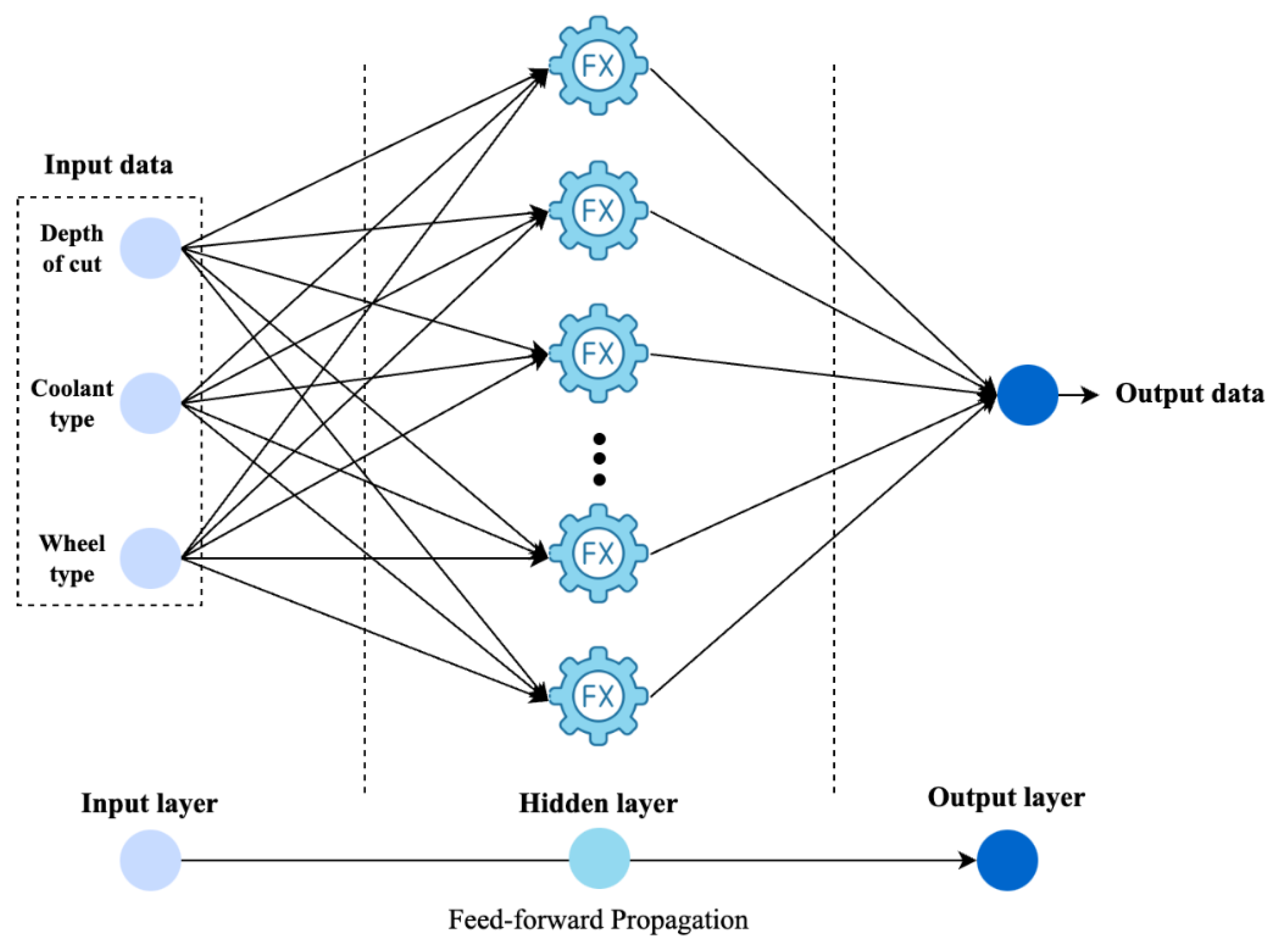
Artificial Neural Networks (ANNs) have been effectively used for many application problems, such as function approximation and classification; as universal approximators, ANNs are especially helpful as function approximators since they don't require prior knowledge of the input data distribution [59]. Figure 4 depicts a schematic of an Artificial Neural Network (ANN).

A Multi-Layer Perceptron (MLP), a feed-forward neural network that associates sets of input data with suitable outputs, is the foundation of the implemented ANN structure [60]. As seen in Figure 4, this structure consists of an input layer, an output layer with a single node, and a single hidden layer with variable nodes. Activation functions are essential components of Artificial Neural Networks (ANNs) because they facilitate the learning and comprehension of intricate and non-linear mappings between inputs and outputs. While there are more than ten activation functions available in the literature [61,62], the ReLU activation function has proven to perform adequately in this study.

Similar to other machine learning techniques, Artificial Neural Networks (ANNs) offer superior performance in predicting intricate relationships between related factors. ANNs can be applied to a wide range of issues due to their scalability and flexibility, particularly in mechanical engineering [63,64,65].

2.7. Accuracy Metrics

Several metrics are available for the regression model, which is a nonlinear structure that is a complex relation between input values and output values. In some literature, up to 29 metrics are discussed [66,67] for just regression; however, it is not necessary to work with all of them in order to select the best model. Three primary measures are introduced here, and the current study employed them to provide a comprehensive understanding of performance by comparing metrics that improve model stability and accuracy in the actual world.

A popular statistic for assessing models is the root-mean-squared error (RMSE), especially for normal (Gaussian) errors [68].

The relative ranks of the models are unaffected by taking the root; however, it produces a metric with the same units as the input data, which can be used to conveniently describe the typical or "standard" error for normally distributed errors (Equation 9).

R M S E = \sqrt{\frac{1}{n} \sum_{1}^{n} {(Y_{p r e} - Y_{a c t})}^{2}}

(9)

Another metric that is frequently used as a loss function in some literature to indicate the mean error in the prediction process is the Mean Absolute Percentage Error (MAPE), which is a measure of the extent of absolute error in percentage terms [67].

M A P E = \frac{1}{n} \sum_{1}^{n} \frac{|Y_{p r e} - Y_{a c t}|}{Y_{a c t}} \times 100

(10)

When used to nonlinear regression models or other nonlinear techniques, the Coefficient of Determination (R²) becomes highly complicated, as the result does not necessarily fall between 0 and 1 and can even be negative.

This problem affects the dependability of (R²) in nonlinear regression, a point raised by some scholars [69]. Eight distinct formulae for (R²) that are present in the literature are discussed by Kvålseth [70], who also points out how they differ, what confusion they produce, and frequent mistakes that may be made while using them. Nevertheless, the common formula (Equation 11) measures the "goodness of fit" and, when combined with other metrics, offers a clear picture of the precision and stability of the applied model [71].

R^{2} = 1 - \frac{\sum_{1}^{n} {(Y_{p r e} - {\bar{Y}}_{p r e})}^{2}}{\sum_{1}^{n} {(Y_{a c t} - {\bar{Y}}_{a c t})}^{2}}

(11)

In equations 9, 10, and 11, the values denoted by

Y_{a c t}

Y_{p r e}

{\bar{Y}}_{a c t}

, and

{\bar{Y}}_{p r e}

are the actual and expected values, actual and predicted mean values, respectively.

The evaluation was based on their R2 and root mean square error (RMSE) score values and mean absolute percentage error (MAPE) [10]. The models were trained using machine learning algorithms using the MATLAB regression learner tool.

2.8. Structure of Study

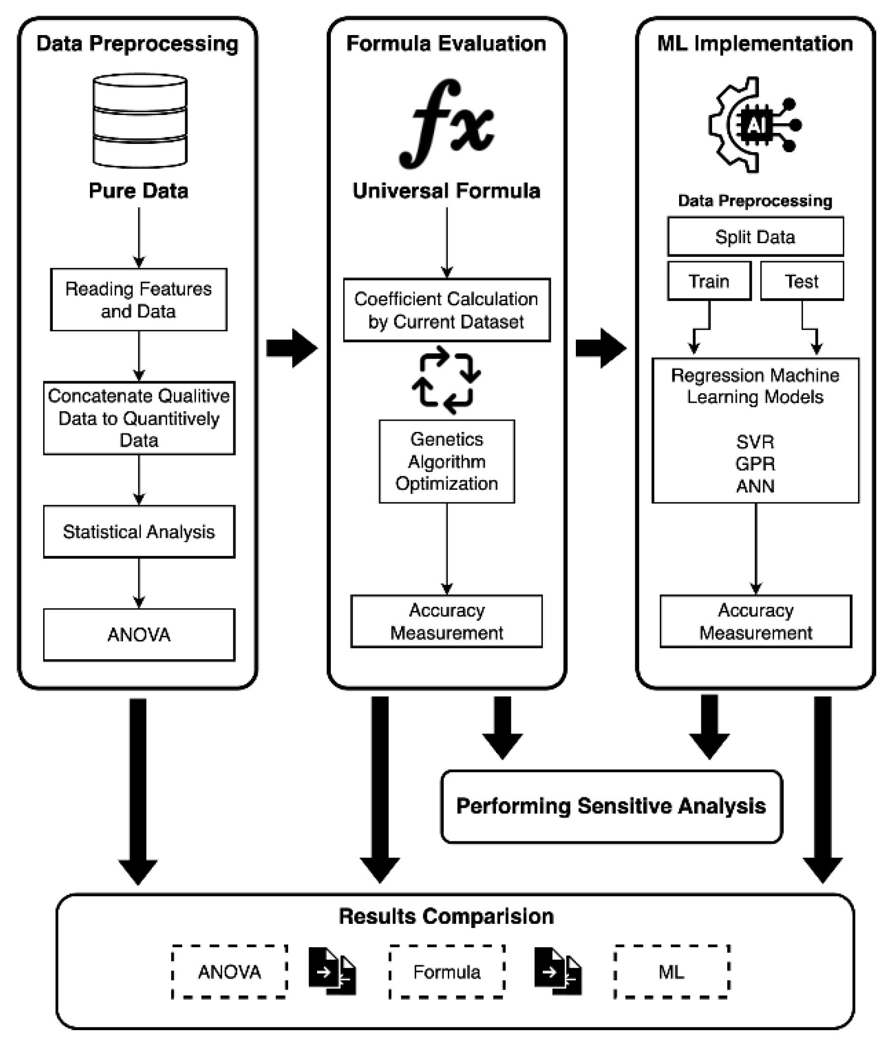
The current study is a multi-disciplinary research project that consists of two distinct fields: manufacturing grinding and machine learning approaches. This integration aligns with the realm of digitalization and sustainability solutions.

To carry out the research, the current study consists of five distinct parts, which are illustrated in Figure 5. The first part (data preprocessing) involves reading data, concatenating (decoding) qualitative inputs to quantitative (coolant type and grinding wheel types), and implementing primary statistical analysis and ANOVA to identify the influence of each parameter on the final outputs (surface roughness and grinding force). The second part (Formula Evaluation) includes a novel formula generalization with genetic algorithm optimization to provide the direct and analytical solution between input and output parameters available in the full dataset, and also providing accuracy analysis to identify the performance of the proposed formula. The third part (ML Implementation) includes the development of the ML model, optimization algorithm, and implementing all three mentioned methods (SVR, GPR, and ANN) to the proposed dataset after splitting it into train and test portions. Then, accuracy metrics calculated the performance of each model and reported separately, especially based on different coolant solutions as promising study parameters. The fourth step is implementing global sensitivity analysis, which uses a model-dependent approach to identify the most and least influential parameters on the final solution (both for surface roughness and grinding forces). Finally, in the last step (fifth one), all the implementations are compared together to provide better insight into the flow of current digitalization implementation.

3. Results and Discussion

3.1. Statistical Analysis and ANOVA

At first glance, statistical analysis is crucial for the current investigation. The dataset comprises 84 sets of grinding process data, which include only one numerical value: the removal rate. Additionally, there are four types of coolant and three different grinding wheels, which are qualitative data associated with the grinding process. During the process, the overall force in the tangential and normal directions was measured, and at the end, the surface roughness (R_z) was recorded. Table 4 provides an overview of all the data collected during the process.

However, implementing statistical or analytical procedures like ANOVA on qualitative data is impossible. Therefore, encoding qualitative data to quantitative representation is necessary. In this study, the four different coolants (dry, MQL model 1, MQL model 2, and fluid) are assigned integer values of 1, 2, 3, and 4, respectively. Similarly, the three types of grinding wheels (Al₂O₃ 180K6, Al₂O₃ 80L6, and 120I8) are assigned integer values of 1, 2, and 3, respectively.

Table 5 presents a primary statistical analysis of the entire dataset. It is crucial to note that for any future investigations, such as machine learning algorithms, the input data (predictors) should be within the same range of minimum and maximum values. The predicted output accuracy and error are measured by the mean value of real predictors like Rz.

In many applications of ANOVA, the sum of squares and p-values are the most relevant outputs, while other values are intermediate steps leading to the p-values, which indicate the results of significance tests. Therefore, the p-value is the key result to consider. However, it is customary to present all computed data in a table to support claims of statistical significance in ANOVA. Each hypothesis is tested using an F-test, which compares the mean square for the source of variation (large when the source significantly affects the measurement) to the error mean square. To determine if a source of variation has a significant effect, examine its p-value. If the p-value is sufficiently small, such as p < 0.05, the effect is considered significant [72].

The ANOVA results for different response variables, shown in Table 6, Table 7, and Table 8 for surface roughness (Rz), grinding force in the tangential direction (F_t), and in the normal direction (F_n), respectively, clearly indicate that all the predictors (input values) significantly affect the responses, as evidenced by p-values below 5%. This suggests that new parameters, such as types of coolant and grinding wheel, will significantly impact the output variables in each test. However, ANOVA does not quantify the extent of each variable's effect. Therefore, additional methods, such as formula implementation and machine learning, are necessary to systematically measure the impact of each parameter on the output values and to create a platform for predicting new responses based on new predictors.

Table 7. The dataset at a glance.

Input Parameters			Output Parameters
Depth of Cut (µm)	Coolant	Grinding Wheel	F_t (N)	F_n (N)	R_z (µm)
35	3	1	33	55	2.11
5	4	1	1.75	5.35	1.7
65	4	1	48.2	83.66	2.15
15	2	2	11	45	1.1
55	3	2	52	118	1.36
45	4	2	50	74	0.93
65	1	3	65	98	1.82
35	2	3	23.4	45	1.12
55	2	3	44	77	1.34
65	2	3	55	90	1.45
5	4	3	2.5	5.5	0.87
15	4	3	10.3	17.6	0.93

Table 8. Statistical analysis overview of preprocessed dataset, the encoded data highlighted in grey color row.

		Min	Max	Average (Mean)	STD
Inputs	Depth of Cut (µm)	5	65	52.5	30.2
	Coolant	1	4	2.5	1.1
	Grinding Wheel	1	3	2	0.8
Outputs	Force tangential direction (N)	1.8	65.0	30.3	19.3
	Force normal direction (N)	4.8	140.0	60.5	36.8
	Surface Roughness	0.4	4.5	1.6	0.8

Table 9. ANOVA analysis results for surface roughness (Rz).

Parameter	Sum Sq.	d.f.	Mean Sq.	F	P-Value
Removal Rate	4.0	6	0.7	21.0	4.3e^-14 < 5%
Coolant	6.5	3	2.2	68.6	4.6e^-21 < 5%
Grinding Wheel	0.9	2	0.5	14.2	6.2e^-6 < 5%
Error	2.3	72	0.03
Total	13.7	83

Table 10. ANOVA analysis results for grinding force (F_t).

Parameter	Sum Sq.	d.f.	Mean Sq.	F	P-Value
Removal Rate	54128.8	6	9021.5	361.3	1.2e^-51 < 5%
Coolant	2765.8	3	921.9	36.9	1.5e^-14 < 5%
Grinding Wheel	1600.9	2	800.46	32.1	1.1e^-10 < 5%
Error	1798	72	24.97
Total	60293.5	83

Table 11. ANOVA analysis results for grinding force (F_n).

Parameter	Sum Sq.	d.f.	Mean Sq.	F	P-Value
Removal Rate	258886.4	6	43147.7	149.6	1.4e^-38 < 5%
Coolant	4494.7	3	1498.2	5.3	0.003 < 5%
Grinding Wheel	43072.8	2	21536.4	74.7	2.8e^-18 < 5%
Error	20773	72	288.5
Total	327226.9	83

3.2. GA and Formula Generation

The Genetic Algorithm (GA) is an iterative process that starts with an initial value and aims to find an optimized solution by minimizing a predefined cost function. In this implementation, the cost function is the squared mean value error, as defined in Equation 4. The GA iterates until it reaches the minimum threshold for the cost function value, which in this case is below 0.001 after 20 iterations. The final simplified formulas for each response—surface roughness, grinding force in the tangential direction (F_t), and grinding force in the normal direction (F_n)—are provided in Equations 12, 13, and 14, respectively. The accuracy metrics are summarized in Table 12.

The obtained equations demonstrate that all input variables significantly affect the output responses, as none were removed from the equations. The coefficients are substantial, indicating that even the interactions between variables are important and cannot be ignored.

From Table 12, although the R² value for surface roughness is around 0.55 and for grinding force in both directions (tangential and normal) is more than 0.6, the MAPE is quite high, exceeding 28%. This indicates that using these equations requires more careful consideration. However, the equations do provide a clear analytical approach for defining the relationship between removal rate and other variables. By implementing further optimization processes with different methods, it is possible to achieve better solutions. Furthermore, although this sophisticated implementation establishes a pioneering relationship between feature parameters (such as depth of cut, types of coolant, and types of grinding wheel) and response variables like surface roughness, it is highly dependent on the provided dataset.

\begin{array}{l} R_{z} = 0.22 x_{r} - 3.03 x_{c} - 0.94 x_{w} + x_{r}^{- 7.33} + x_{c}^{0.35} + x_{w}^{- 5.17} + \frac{2.44}{x_{r}} + \frac{3.18}{x_{c}} - \frac{4.64}{x_{w}} - 0.02 x_{r} x_{c} \\ + 0.93 x_{c} x_{w} - 0.04 x_{r} x_{w} - 0.06 \frac{x_{r}}{x_{c}} + 3.13 \frac{x_{c}}{x_{w}} - 0.10 \frac{x_{r}}{x_{w}} - \frac{8.84}{x_{r} x_{c}} + \frac{1.83}{x_{x} x_{w}} \\ + \frac{2.79}{x_{r} x_{w}} \end{array}

(12)

\begin{array}{l} F_{t} = 0.06 x_{r} + 3.29 x_{c} - 2.78 x_{w} + x_{r}^{0.61} + x_{c}^{1.30} + x_{w}^{- 0.37} + \frac{5.00}{x_{r}} + \frac{2.01}{x_{c}} - \frac{5}{x_{w}} + 0.10 x_{r} x_{c} \\ - 1.06 x_{c} x_{w} + 0.005 x_{r} x_{w} + 0.46 \frac{x_{r}}{x_{c}} - 3.94 \frac{x_{c}}{x_{w}} - 0.10 \frac{x_{r}}{x_{w}} + \frac{5.00}{x_{r} x_{c}} + \frac{0.21}{x_{x} x_{w}} \\ + \frac{4.97}{x_{r} x_{w}} \end{array}

(13)

\begin{array}{l} F_{n} = 2.97 x_{r} + 3.22 x_{c} - 1.41 x_{w} + x_{r}^{0.60} + x_{c}^{- 4.94} + x_{w}^{- 0.16} - \frac{4.98}{x_{r}} + \frac{5.00}{x_{c}} - \frac{2.45}{x_{w}} \\ - 0.08 x_{r} x_{c} - 0.25 x_{c} x_{w} - 0.50 x_{r} x_{w} - 0.19 \frac{x_{r}}{x_{c}} - 4.99 \frac{x_{c}}{x_{w}} - 1.17 \frac{x_{r}}{x_{w}} \\ - \frac{5.00}{x_{r} x_{c}} + \frac{5.00}{x_{x} x_{w}} - \frac{4.97}{x_{r} x_{w}} \end{array}

(14)

3.3. Surface Roughness

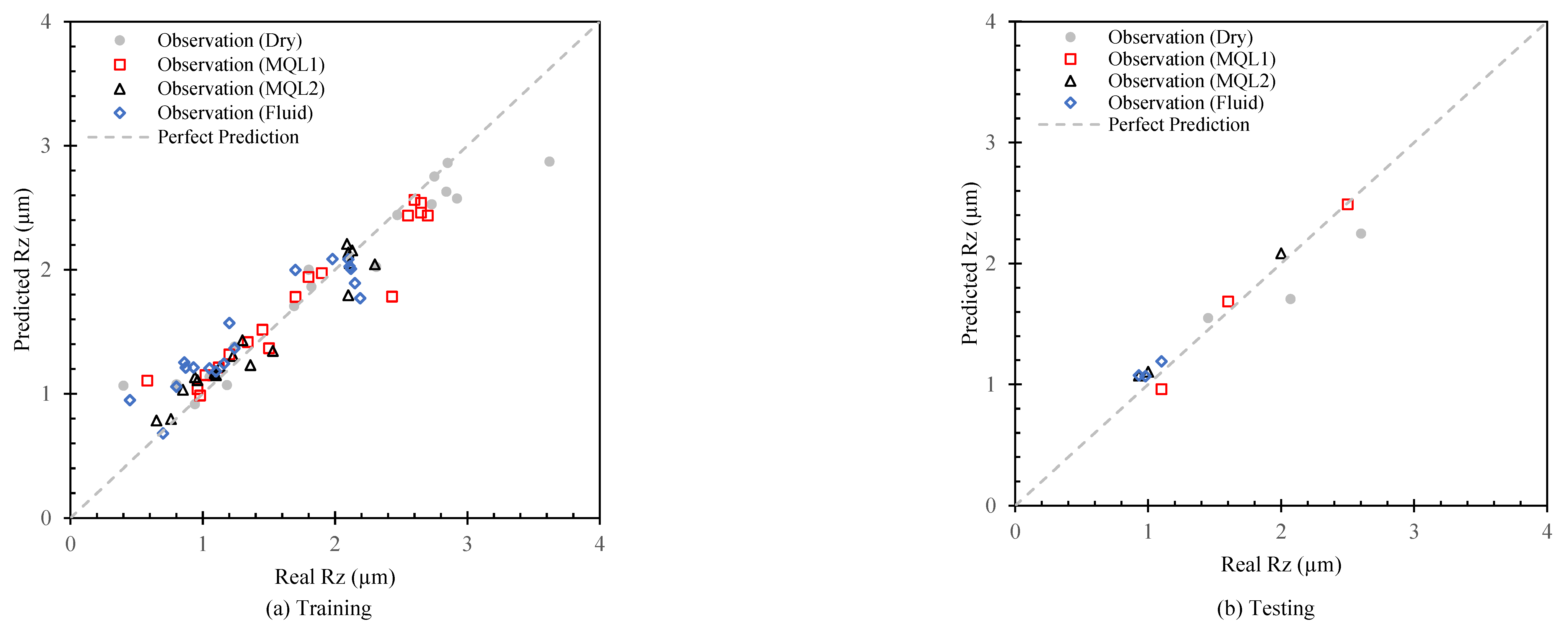
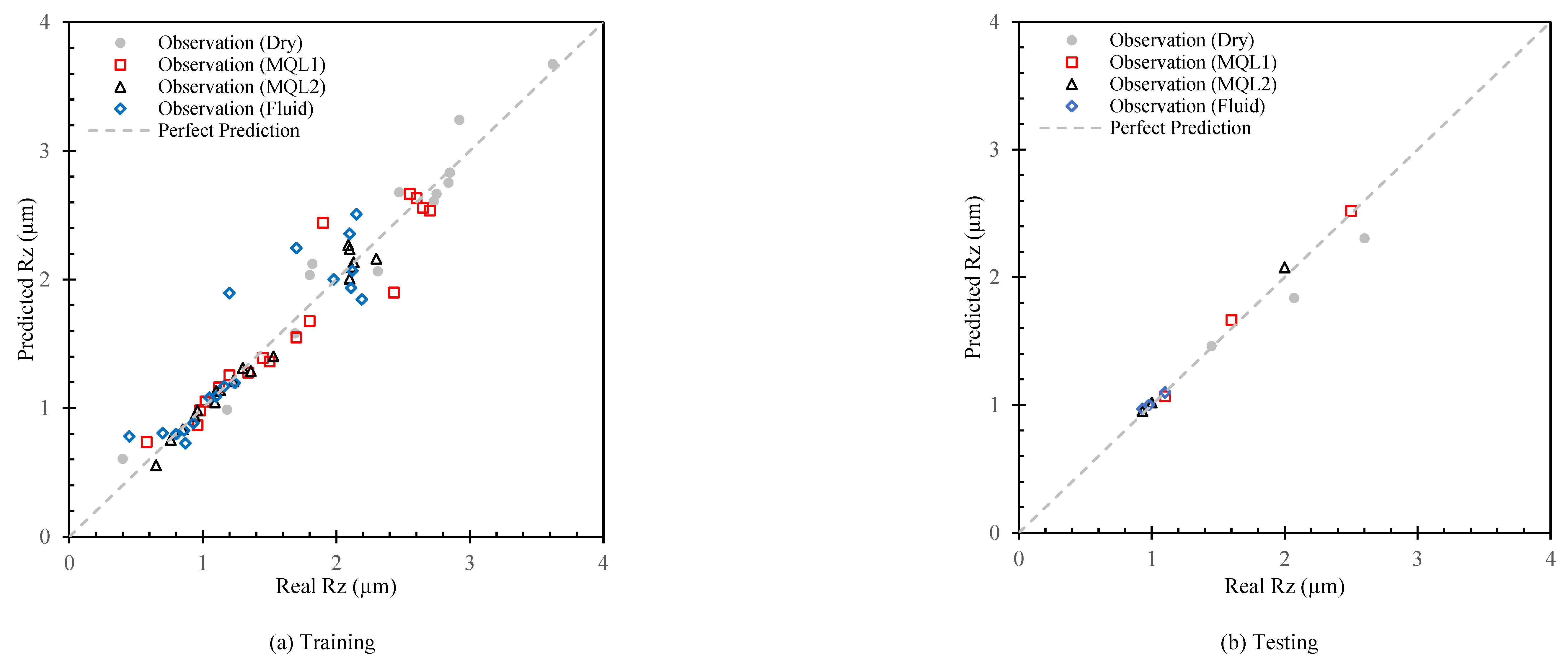
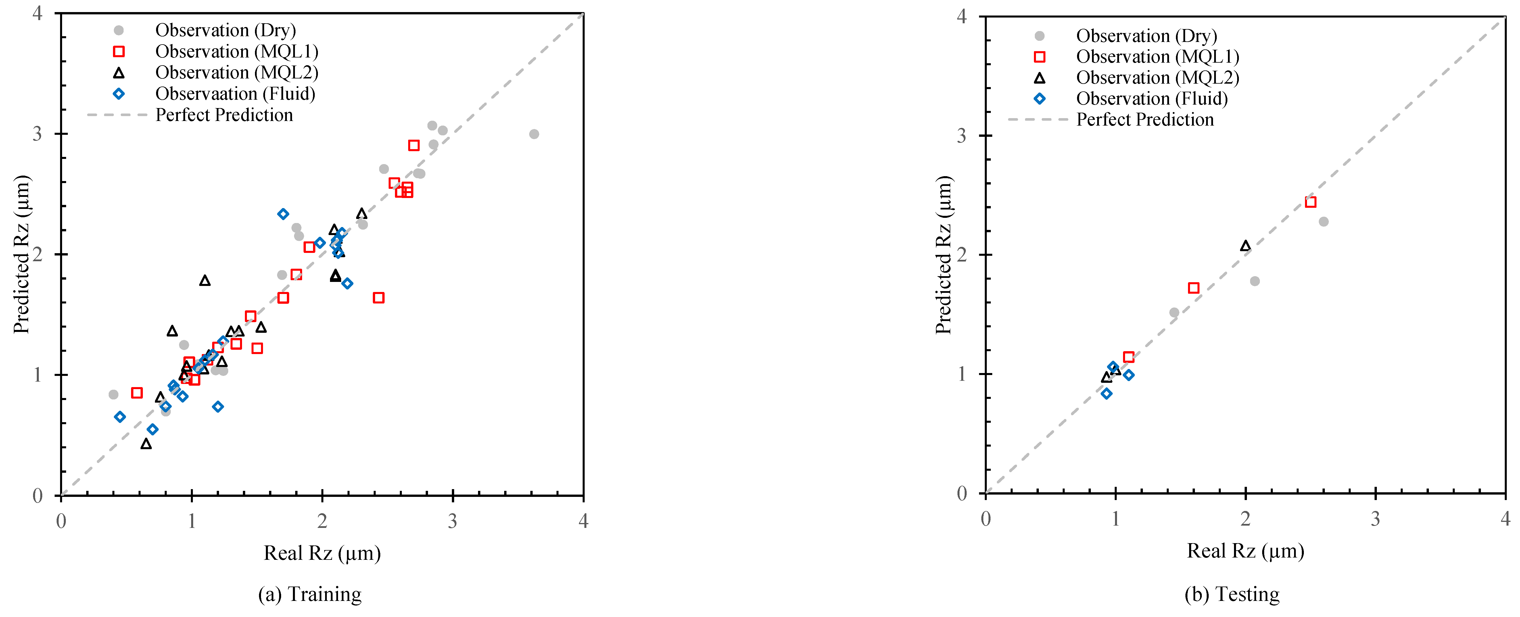
The results of implementing machine learning algorithms on the dataset with respect to surface roughness are illustrated in Figure 6, Figure 7 and Figure 8 for the SVR, GPR, and ANN methods, respectively. Before implementing the ML models, the dataset was split homogeneously into training and test sets with equal distribution based on coolant type. The main focus of this study, besides implementing ML models, is to investigate the effects of coolant type on the accuracy and stability of each model. Therefore, each part of the dataset includes 21 sets of data for each coolant. Randomly, three data points were selected, resulting in the training portion containing 72 sets of data and the test portion containing 12 sets of data. All 72 data points were used for training each model with hyperparameter optimization based on the Bayesian algorithm. The final trained version of each model was then implemented on the test data, and all results were shown based on coolant type in Figure 6, Figure 7 and Figure 8.

From Figure 7a,b, the correlation between real and predicted data in training is lower than in other methods, visually showing that both MQL coolants perform better than other coolant types, with a clearly lower distribution. Furthermore, the accuracy metrics for the GPR method clearly indicate the best solution compared to other ML implementations, as it provided the highest R² value. For the training process, the dry and MQL1 coolants yielded the best R² value of 0.93, while the mean absolute percentage error (MAPE) for the dry coolant is lower than for MQL (4.58% and 5.12%, respectively). In the second stage, the fluid coolant also provided acceptable values with an R² of 0.87 and a MAPE of 4.64%. However, for MQL2, the R² is 0.76 and the MAPE is 6.91%, which is somewhat reasonable for the current study.

The SVR method, which has a negative R² in the training process, is not acceptable, although it has a lower MAPE value under 7% for MQL2 and fluid coolants, or in the testing process, it provided reasonable solutions.

The ANN implementation in a single-layer configuration for the training process for dry and MQL1 coolants also provided acceptable solutions (with R² values of 0.89 and 0.77 and MAPE values of 9.2% and 12.8%, respectively). However, the values for MQL2 and fluid coolants are far from the acceptable range, with R² values of 0.54 and 0.46 and MAPE values of 7.9% and 7.6%, respectively.

The results from the testing process indicate how well the implemented methods can predict unseen data within an acceptable range. From Figure 6(b), Figure 7(b), and Figure 8(b) for the testing process of SVR, GPR, and ANN, respectively, it is challenging to determine which implementation provided better results without considering the accuracy metrics for the testing data. Table 13 and Table 14 clearly show that the GPR method provided the best testing solution without any hesitation. For dry, MQL1, and fluid coolants, the R² values are 1.0, 0.95, and 0.99, respectively, which are the best results. However, MQL2, with an R² of around 0.57, introduces some variability in the final result. Furthermore, the average accuracy for dry, MQL1, and fluid coolants in the testing process is more than 97%, indicating that the GPR method can predict surface roughness with reasonable accuracy and stability.

In contrast, the ANN method only provided an acceptable solution for fluid coolant, with an R² of 0.98 and a MAPE of around 3.6%. The SVR method showed R² values of 0.87 and 0.82 for fluid and MQL1 coolants, respectively. However, both methods had negative R² values for MQL2 and dry coolants, indicating that these two methods, with the selected optimized hyperparameters, are not suitable for any prediction procedure for the current dataset and require further optimization.

3.4. Grinding Force Tnagential Direction (F_t)

The provided dataset also includes grinding force in the tangential and normal directions, which specifically influences surface roughness and surface temperature; however, the temperature data was not provided. In this section, the considered machine learning methods were retrained to predict grinding force, first in the tangential direction (discussed in this section) and then in the normal direction (discussed in the next section). Like the previous section, the dataset was split homogeneously into training and test sets, with the training portion containing 72 sets of data and the test portion containing 12 sets of data. All 72 data points were used for training each model with hyperparameter optimization based on the Bayesian algorithm.

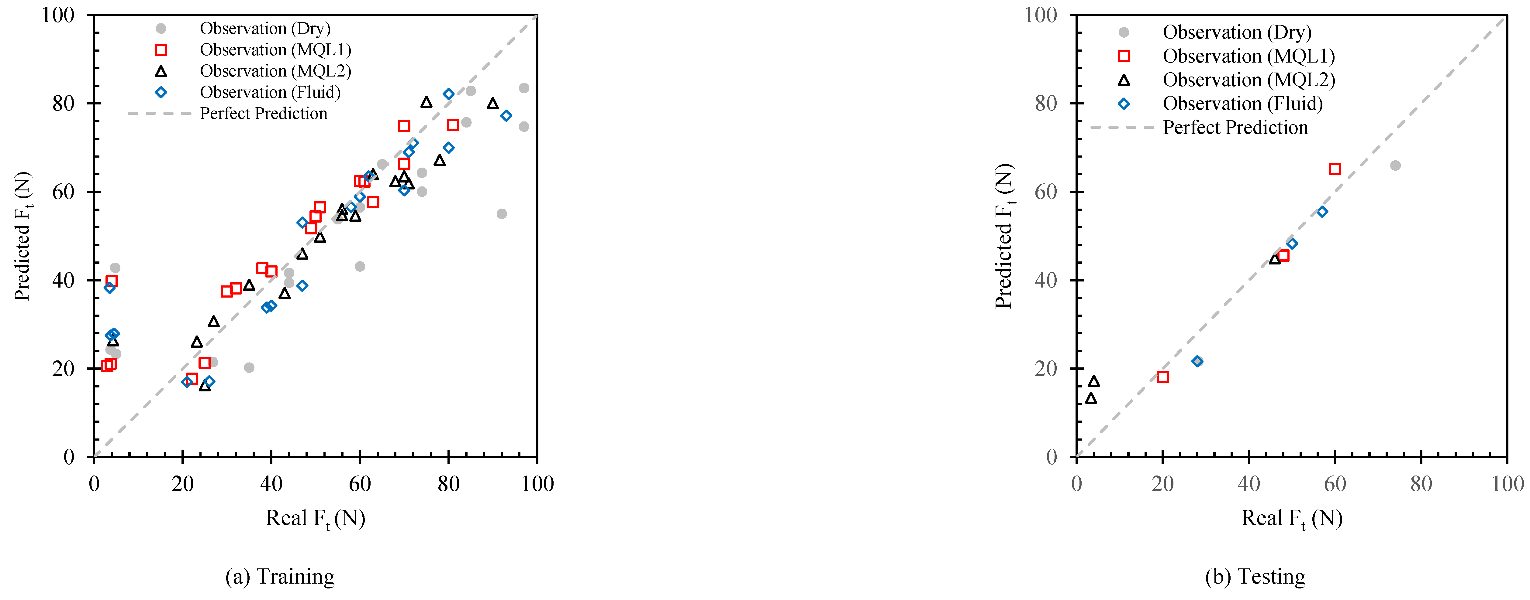
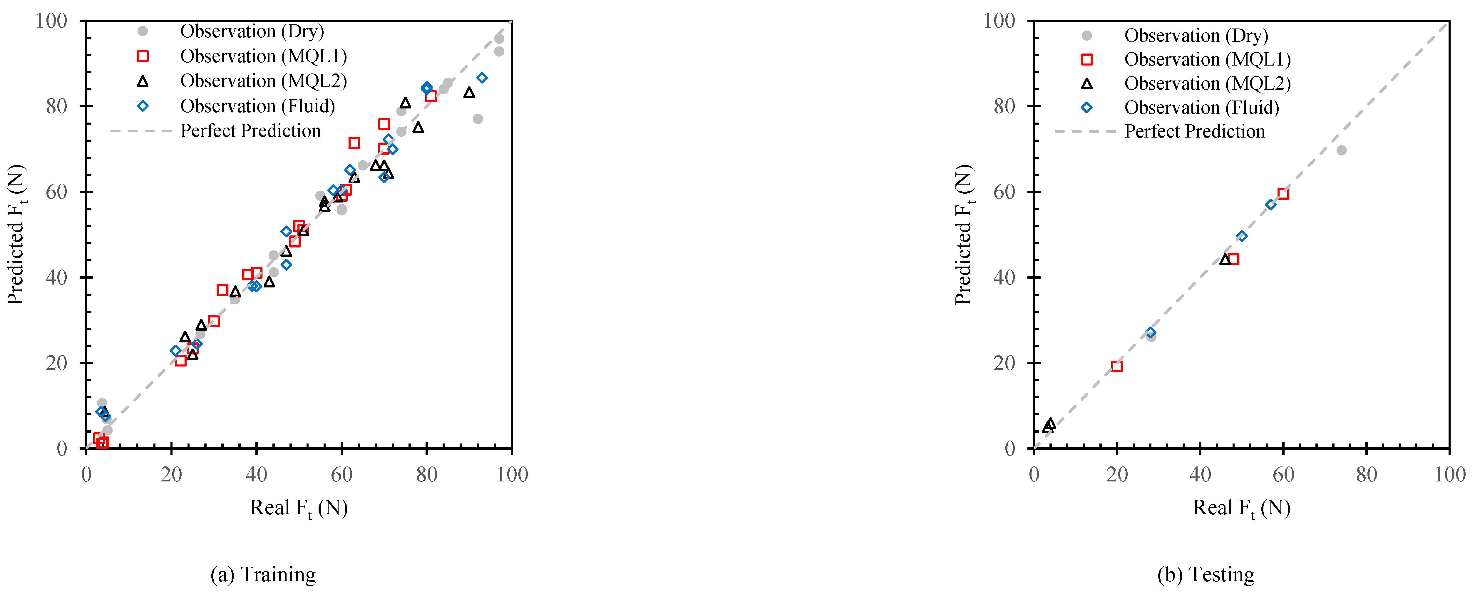
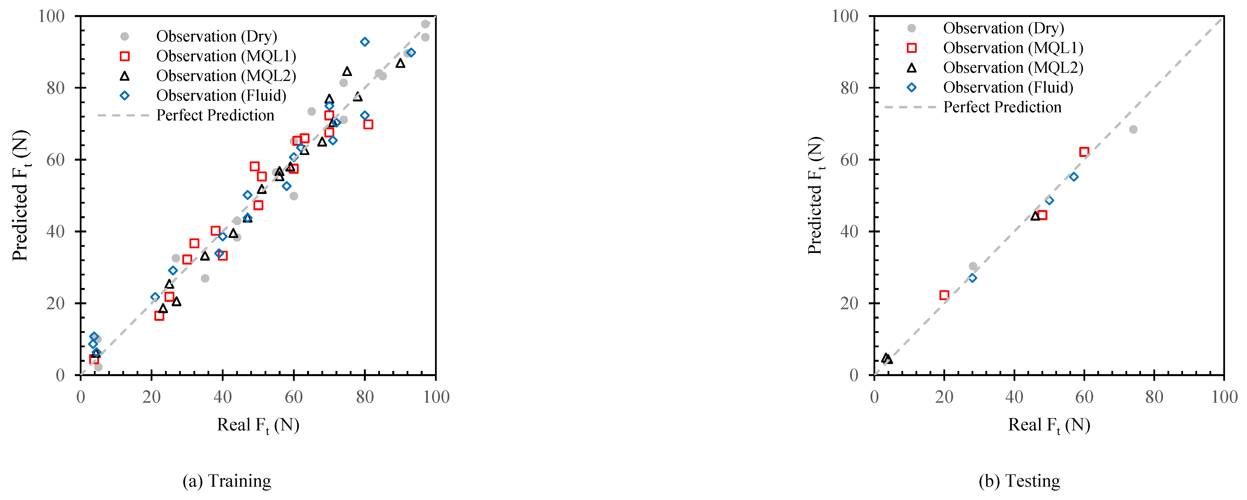
The results of implementing machine learning algorithms on the dataset with respect to grinding force in the tangential direction are illustrated in Figure 9, Figure 10, and Figure 11 for the SVR, GPR, and ANN methods, respectively. Before implementing the ML models, the dataset was split homogeneously into training and test sets with equal distribution based on coolant type. This illustration provides better insight into the influence of coolant type specifically on grinding force.

From Figure 9(a) to Figure 11(a), it is clear that both GPR and ANN methods have lower data correlation with the perfect prediction line, with MQL2 in the GPR method (illustrated with a black triangle mark) having the lowest correlation in the training process. However, making judgments from a visual graph without clear numerical data seems odd, so Table 15 and Table 16 tabulate the accuracy metrics of the training and testing solutions.

It is clearly shown that both GPR and ANN implementations have reasonably robust solutions based on R² values, which are higher than 0.97 for all coolant types in GPR and higher than 0.96 for ANN. However, the MAPE value is a bit challenging in this scenario. In the training procedure for grinding force in the tangential direction, the MAPE value for the GPR method is 9.9% and 7.8% for dry and MQL2 coolants, respectively, while this value for MQL1 is about 26% and 65% for MQL1 and fluid, respectively, which needs more consideration for using these methods for these coolant types. In contrast, the MAPE value for ANN is reasonably high, reaching around 20.5% and 45% for dry and MQL1, respectively, which shows that although the ANN method is a stable machine learning solution, the accuracy results for all coolant types did not provide a valuable solution for any future consideration and digital predictor platform.

Additionally, the SVR method has R² training values ranging from 0.3 to 0.93 for different coolants, indicating that overall, the SVR does not provide a robust network configuration.

Figure 9(b) to Figure 11(b) illustrate the testing procedure implemented on a part of the dataset that was not used for training. This action measures the ability of the trained network to predict unseen data. The results in Figure 9(b) to Figure 11(b) are quite similar, making it difficult to judge the accuracy of these methods solely from the figures. However, it is clearly evident that the SVR method did not provide an acceptable solution, as its data correlation is higher than that of the other methods.

Table 15 and Table 16 in the test section show that both the GPR and ANN methods, with R² values greater than 0.97 for all coolant types, provided a sophisticated and stable solution. The MAPE values are lower than 5.2% for dry, MQL1, and fluid coolants (with the fluid coolant achieving a MAPE of about 1.3%), which is overall acceptable. However, the MAPE value for MQL2 is somewhat high (about 24%) and should be considered when using this method for MQL2 data.

The ANN method also shows MAPE results under 7.1% for dry, MQL1, and fluid coolants, indicating that this method is also suitable for any further data prediction. It is worth noting that, like the GPR method, the ANN method reaches a high MAPE value for MQL2, around 15.5%.

3.5. Grinding Force Normla Direction (F_n)

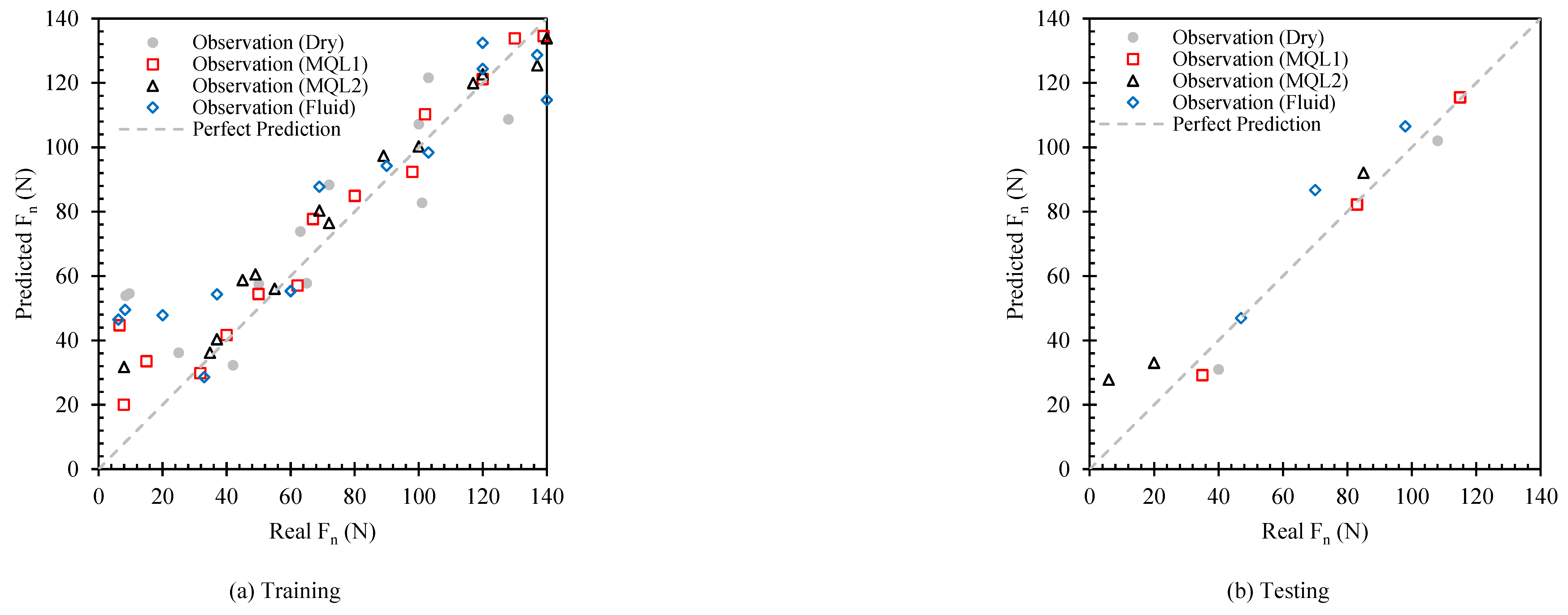
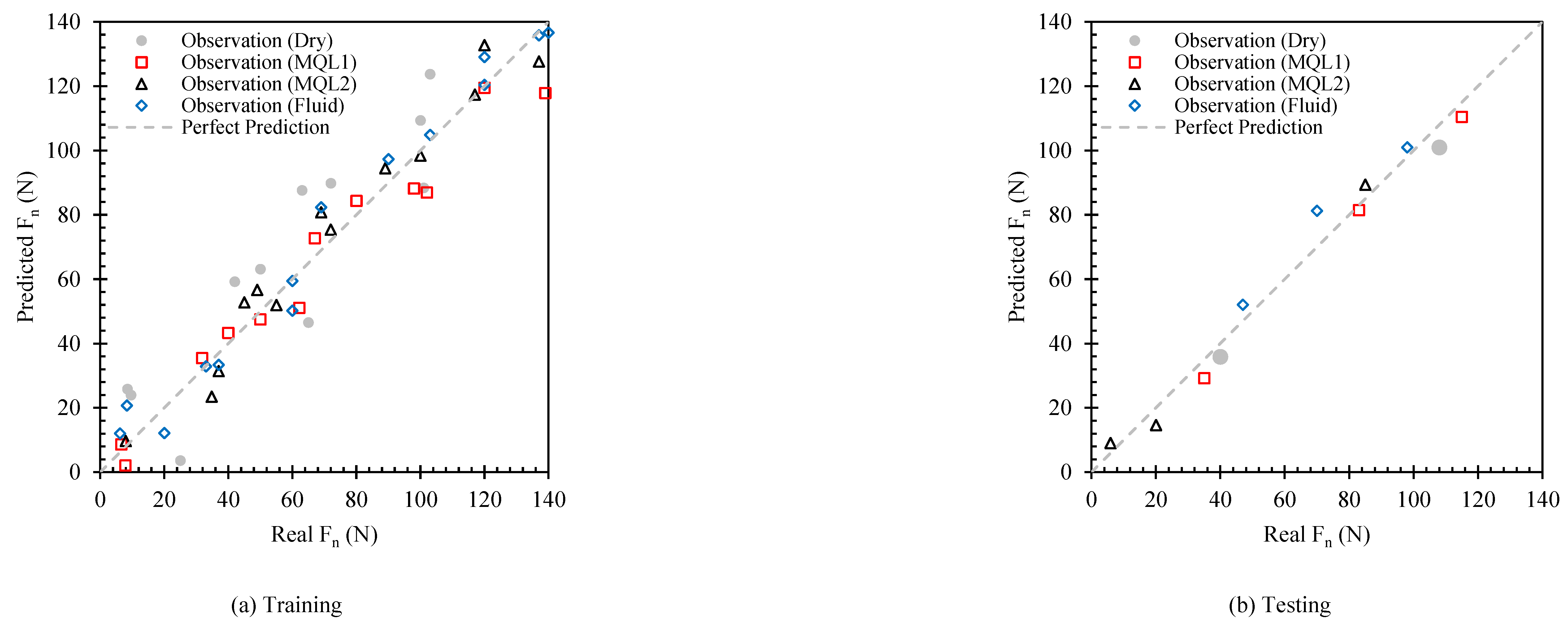
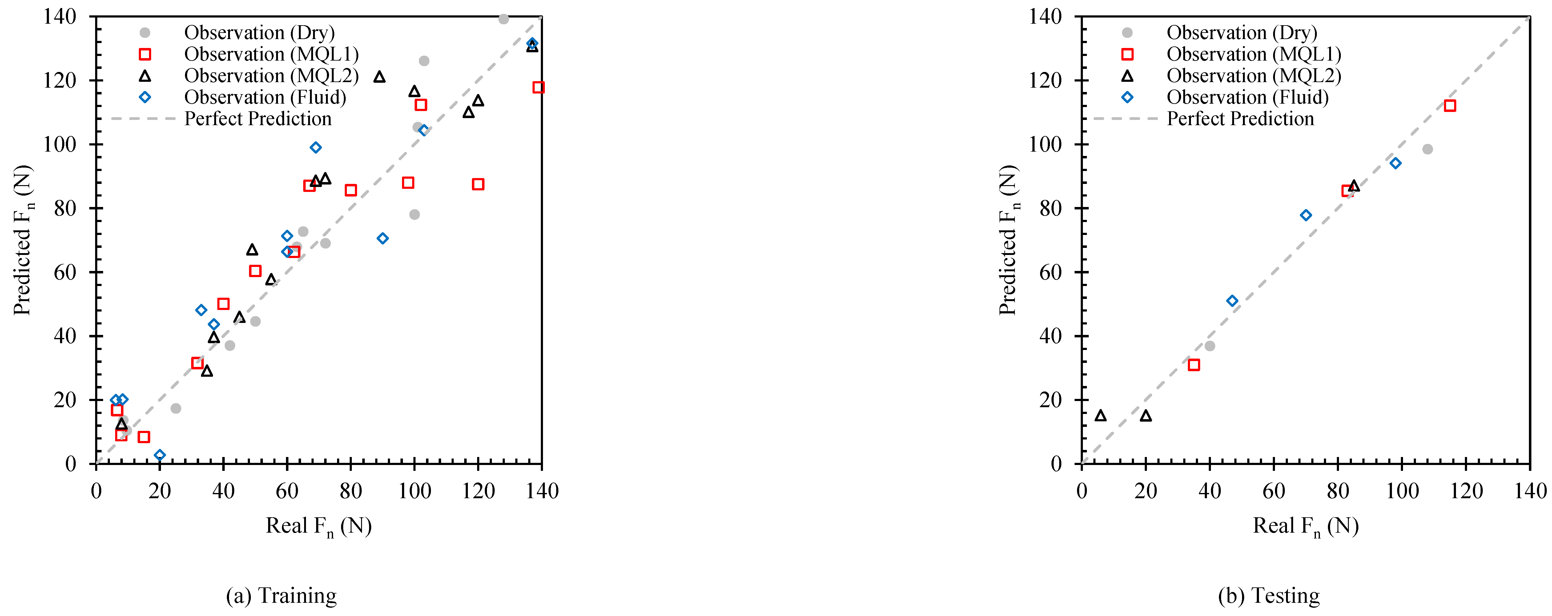
The same data for grinding force in the normal direction is also available, and the same implementation conducted for the tangential direction was applied to the normal direction. The final results are illustrated in Figure 12, Figure 13, and Figure 14 for the SVR, GPR, and ANN methods, respectively. The portion size for training and testing implementation is similar to the previous section (72 sets of data for training and 12 sets of data for testing).

Clearly, from the training results (Figure 12(a), Figure 13(a), and Figure 14(a)), the data variation for the normal direction is more than for the tangential direction. Because of this, the correlation between real data and predicted data is high, and the data distribution around perfect prediction seems unsatisfactory. Table 17 and Table 18 provide accuracy metrics results to give better insight into the models’ implementation.

For the training process, it is clearly shown that the GPR method, with an R² of more than 0.90 compared to other methods, provided robust machine learning implementations. Furthermore, the R² for MQL2 and fluid coolant is 0.96 and 0.98, respectively, while the MAPE results are 11.3% and 14.6%, respectively, which is reasonably acceptable in the engineering field. However, for dry and MQL1 coolant, although the R² is high and acceptable, the MAPE is absolutely high (54% and 89%), indicating that for this type of coolant, the learning process was not conducted successfully and needs more training or other optimization processes.

For the ANN method, the R² results vary from 0.8 to 0.92, which is acceptable for this type of jittering data. While MQL2 has an R² of around 0.89, its MAPE is 21%. The R² value for fluid coolant is 0.92, while the MAPE is 53%, making it hard to make a robust decision for selecting an appropriate method. For dry coolant, the R² is 0.8 and the MAPE is about 18%.

The SVR method, like other implementations in this study, could not provide a reasonable solution. The R² varies from 0.43 to 0.89, clearly showing that the SVR’s robustness for some coolant methods is absolutely problematic. Although the MAPE results for the SVR method in the training process are lower than other implementations, the method’s robustness confirms that the training process could not provide a stable solution.

From the training results, it is clear that the test results illustrated in Figure 12(b), Figure 13(b), and Figure 14(b) for the SVR, GPR, and ANN methods, respectively, are not reasonably perfect. Therefore, the accuracy metrics in Table 17 and Table 18 in the test section provide all the necessary results for the final judgment. Notably, the GPR results are the best among the others. The R² for GPR in the test section is about 0.98 for dry, MQL1, and MQL2, while the R² for fluid coolant is 0.87, which is acceptable. The MAPE results are also around 9% for dry, MQL1, and fluid, while the MAPE for MQL2 is slightly higher at around 25%.

For the ANN method in the testing procedure, the R² is also high, exceeding 0.94 for dry, MQL1, and MQL2, while the R² for fluid is about 0.86, which is acceptable. The MAPE results do not exceed 11.6% for dry, MQL1, and fluid, while the MAPE for MQL2 is 54%, indicating that using the ANN method for MQL2 requires some consideration and attention.

The test results for SVR in this situation are not acceptable, with R² values ranging from 0.64 to 0.99, and the MAPE for MQL2 is extremely high at around 42%. Therefore, this method will not be accepted for any further consideration.

3.6. Sensitivity Analysis

The sensitivity analysis results for surface roughness and grinding force in the tangential and normal directions are illustrated in Figure 15, Figure 16, Figure 17, Figure 18, Figure 19 and Figure 20. The effects of input parameters on surface roughness are investigated in Figure 15 and Figure 16. Figure 15 illustrates the effects of depth of cut (5, 35, and 65 µm) for each coolant solution on surface roughness, considering the Al2O3 80L6(2) grinding wheel. The figure clearly shows that surface roughness values increase as the depth of cut increases. According to the current trend, the GPR and ANN methods predict the real values accurately with low absolute error, while the SVR method does not provide sufficient results.

Another interesting result from Figure 15 is that the MQL1 coolant provides the lowest surface roughness value, as proven by real values and the GPR and ANN implementations. In contrast, the Dry method results in the highest surface roughness, which is expected from industrial results.

Figure 16 specifically studies the effects of different grinding wheels at different depths of cut (5, 35, and 65 µm), with the cooling method fixed at MQL1 (the best coolant in this study). It clearly shows that surface roughness increases with the depth of cut for all grinding wheel types. Overall, the GPR and ANN prediction methods can reasonably track the real values with the lowest error. Furthermore, the Al2O3 80L6(2) grinding wheel achieves the lowest surface roughness at a 5 µm depth of cut among the others. At a 65 µm depth of cut, the surface roughness values for all grinding wheels are similar, with negligible differences.

For grinding force in the tangential and normal directions, Figure 17 and Figure 18, respectively, illustrate the trend changes with respect to different cooling methods while the grinding wheel remains Al₂O₃ 80L6(2). It clearly shows that the force increases dramatically in both directions as the depth of cut increases from 5 to 35 µm, and this increasing trend in grinding force continues as the depth of cut increases to 65 µm.

From the mentioned figures, the value of force in the tangential and normal directions does not change significantly at each depth of cut for different cooling methods. However, with a more specific comparison, the value of grinding force for MQL1 is lower than the others, although identifying the difference is somewhat complicated. In contrast, the dry cooling method results in higher grinding force, which is expected from industrial implementations.

A noteworthy finding from Figure 17 and Figure 18 is the notable consistency observed between the predicted values produced by the ML models (GPR and ANN). In other words, this harmonious alignment in grinding force prediction in both directions, achieved through the GPR, ANN models, highlights the models’ robustness, precision, and dependability in reflecting real-world scenarios within the specified range.

For the final consideration in this section, comparing the results illustrated in Figure 17 and Figure 18 clearly shows that the overall value of grinding force in the normal direction is significantly higher than the grinding force in the tangential direction at all depths of cut and for all coolant methods.

Figure 19 and Figure 20 present the final results of grinding forces in the tangential and normal directions with respect to different grinding wheels, while the coolant method is set to MQL1. The trend shows an increase in grinding force values as the depth of cut increases. Although the absolute value of each grinding force at each depth of cut appears to be similar, the 120I8(8) grinding wheel achieves slightly lower grinding force values. Additionally, the grinding force in the normal direction is significantly higher than in the tangential direction due to the nature of the grinding process.

4. Conclusions

Modeling the relationship between various direct effective parameters on grinding surface roughness and grinding force is not mandatory to consider simultaneously and is not implemented with respect to cooling type and grinding wheel. The current study provides a novel insight by incorporating these qualitative parameters alongside other quantitative ones, such as depth of cut, as considered in the previously mentioned published study. It is crucial to conduct model-dependent general sensitivity analysis, like ANOVA, which is well-known in the literature. The illustrated results show that the P-value for all mentioned parameters, especially encoded qualitative ones, is under 5%, indicating that all parameters have significant effects on the final results (including surface roughness and grinding force). However, ANOVA does not provide sufficient information about the actual relationship between inputs and outputs.

In the next stage, a novel analytical formula generation was implemented, which completely defines the relationship between input parameters and outputs and also considers the interaction between input parameters, which directly affects the final output. The resultant provided 18 unknown formula coefficients, which were solved by a genetic algorithm optimization procedure based on the provided dataset and mean absolute error (MSE) as the cost function. The final results provided three different analytical formulas, which are quite complicated but show that all input parameters and their interactions have direct effects on the final results, as none of the 18 coefficients reached a zero value.

At the end, accuracy metrics were conducted to measure the robustness of these three functions, showing an R² value around 0.55 and mean accuracy around 70%. While this is not highly sophisticated, this novel approach provides good insight into the effectiveness of each input parameter. It is noteworthy to mention that this kind of implementation is not scalable and flexible, as it is highly dependent on the included dataset. Any changes in the size of the data or the addition or removal of any types of data make the final formula worthless. Therefore, it is important to implement methods that are flexible and scalable with low implementation costs.

Based on the literature review, the best universal machine learning methods, which are well-known in the field of regression analysis, were selected and optimized using a Bayesian optimization approach for adjusting hyperparameters. This was done to implement a sophisticated relationship between predictors (depth of cut, types of cooling method, and types of grinding wheel) and response values (surface roughness, grinding force in tangential and normal directions) separately. After the training and testing procedures and measuring accuracy metrics, the GPR method provided the best solution in both the training and testing processes. For surface roughness, the R² value ranged from 0.75 to 1 for testing and from 0.57 to 0.99 for training. Additionally, the effects of cooling type on prediction were measured and reported, with the MQL1 achieving a reliable and robust solution with higher R² values in both the training and testing processes.

The next implementation focused on grinding force in the tangential and normal directions separately. For both implementations, the GPR and ANN models provided acceptable solutions. The GPR model achieved an R² value of around 0.99 with a MAPE of about 10% for training in the tangential direction, and an R² of 0.98 with a MAPE of 14.8% in the normal direction. This performance is slightly better than the ANN model, which had an R² of 0.97 and a MAPE of 8% in the tangential direction, and an R² of 0.92 with a MAPE of 14.2% in the normal direction. However, both methods will be selected for further extended implementation in the realms of digitalization.

The sensitivity analysis was implemented to ensure that the defined input parameters, including surface roughness and grinding force in the tangential and normal directions, have direct effects on the final solution. The sensitivity analysis confirms that the procedure of selecting qualitative parameters and encoding them quantitatively is reasonably important and has direct effects on response values. Additionally, the best machine learning methods selected can follow the trends, which is validated by real values.

Author Contributions

Conceptualization M.J.H. and S.A., Methodology: M.D.A, P.N., and M.S.J; Software: M.G. and P.N.; Visualization: M.S.J. and M.G.; Validation: M.D.A and P.N.; Formal analysis: P.N.; Investigation: M.D.A.; Resources: M.J.H. and S.A.; Data curation: M.J.H., Writing—original draft preparation: M.D.A., P.N. and M.S.J; Writing—review and editing: M.G.; Supervision: M.D.A; Project administration: M.D.A; Funding acquisition: No fund. All authors have read and agreed to the published version of the manuscript.

Funding

This research received no external funding.

Institutional Review Board Statement

Not applicable.

Informed Consent Statement

Informed consent was obtained from all subjects involved in the study.

Data Availability Statement

The original contributions presented in the study are included in the article, further inquiries can be directed to the corresponding author.

Conflicts of Interest

The authors declare no conflicts of interest.

References

Lai, J.K.L.; Shek, C.H.; Lo, K.H. Stainless Steels: An Introduction and Their Recent Developments; Bentham Science Publishers, 2012; ISBN 1-60805-305-9.
Smaga, M.; Boemke, A.; Daniel, T.; Klein, M.W. Metastability and Fatigue Behavior of Austenitic Stainless Steels. EDP Sciences 2018, 165, 04010. [Google Scholar] [CrossRef]
Marshall, P. Austenitic Stainless Steels: Microstructure and Mechanical Properties. 1984.
Chandra, K.; Kain, V.; Tewari, R. Microstructural and Electrochemical Characterisation of Heat-Treated 347 Stainless Steel with Different Phases. Corrosion science 2013, 67, 118–129. [Google Scholar] [CrossRef]
Gonzaga, A.C.; Barbosa, C.; Tavares, S.S.M.; Zeemann, A.; Payão, J.C. Influence of Post Welding Heat Treatments on Sensitization of AISI 347 Stainless Steel Welded Joints. Journal of Materials Research and Technology 2020, 9, 908–921. [Google Scholar] [CrossRef]
Gopan, V.; Wins, K.L.D.; Evangeline, G.; Surendran, A. Experimental Investigation for the Multi-Objective Optimization of Machining Parameters on AISI D2 Steel Using Particle Swarm Optimization Coupled with Artificial Neural Network. Journal of Advanced Manufacturing Systems 2020, 19, 589–606. [Google Scholar] [CrossRef]
Hosseini, S.F.; Emami, M.; Sadeghi, M.H. An Experimental Investigation on the Effects of Minimum Quantity Nano Lubricant Application in Grinding Process of Tungsten Carbide. Journal of Manufacturing Processes 2018, 35, 244–253. [Google Scholar] [CrossRef]
Mayer Jr, J.E.; Fang, G.-P. Effect of Grinding Parameters on Surface Finish of Ground Ceramics. CIRP annals 1995, 44, 279–282. [Google Scholar] [CrossRef]
Winter, M.; Li, W.; Kara, S.; Herrmann, C. Determining Optimal Process Parameters to Increase the Eco-Efficiency of Grinding Processes. Journal of Cleaner Production 2014, 66, 644–654. [Google Scholar] [CrossRef]
Prashanth, G.S.; Sekar, P.; Bontha, S.; Balan, A.S.S. Grinding Parameters Prediction under Different Cooling Environments Using Machine Learning Techniques. Materials and Manufacturing Processes 2023, 38, 235–244. [Google Scholar] [CrossRef]
Mirifar, S.; Kadivar, M.; Azarhoushang, B. First Steps through Intelligent Grinding Using Machine Learning via Integrated Acoustic Emission Sensors. Journal of Manufacturing and Materials Processing 2020, 4, 35. [Google Scholar] [CrossRef]
Guo, W.; Wu, C.; Ding, Z.; Zhou, Q. Prediction of Surface Roughness Based on a Hybrid Feature Selection Method and Long Short-Term Memory Network in Grinding. The International Journal of Advanced Manufacturing Technology 2021, 112, 2853–2871. [Google Scholar] [CrossRef]
Agarwal, S. Optimizing Machining Parameters to Combine High Productivity with High Surface Integrity in Grinding Silicon Carbide Ceramics. Ceramics International 2016, 42, 6244–6262. [Google Scholar] [CrossRef]
Jafarian, F.; Umbrello, D.; Golpayegani, S.; Darake, Z. Experimental Investigation to Optimize Tool Life and Surface Roughness in Inconel 718 Machining. Materials and Manufacturing Processes 2016, 31, 1683–1691. [Google Scholar] [CrossRef]
Lee, E.T.; Fan, Z.; Sencer, B. Real-Time Grinding Wheel Condition Monitoring Using Linear Imaging Sensor. Procedia Manufacturing 2020, 49, 139–143. [Google Scholar] [CrossRef]
Kadivar, M.; Azarhoushang, B.; Klement, U.; Krajnik, P. The Role of Specific Energy in Micro-Grinding of Titanium Alloy. Precision Engineering 2021, 72, 172–183. [Google Scholar] [CrossRef]
Shiliang, W.; Hong, Z.; Juntao, J.; Yunfeng, L. Investigation on Surface Micro-Crack Evaluation of Engineering Ceramics by Rotary Ultrasonic Grinding Machining. The International Journal of Advanced Manufacturing Technology 2015, 81, 483–492. [Google Scholar] [CrossRef]
Wuest, T.; Weimer, D.; Irgens, C.; Thoben, K.-D. Machine Learning in Manufacturing: Advantages, Challenges, and Applications. Production & manufacturing research 2016, 4, 23–45. [Google Scholar] [CrossRef]
Kant, G.; Sangwan, K.S. Predictive Modelling for Energy Consumption in Machining Using Artificial Neural Network. Procedia CIRP 2015, 37, 205–210. [Google Scholar] [CrossRef]
Govindhasamy, J.J.; McLoone, S.F.; Irwin, G.W.; French, J.J.; Doyle, R.P. Neural Modelling, Control and Optimisation of an Industrial Grinding Process. Control Engineering Practice 2005, 13, 1243–1258. [Google Scholar] [CrossRef]
Zhang, Y.; Xu, X. Predicting the Material Removal Rate during Electrical Discharge Diamond Grinding Using the Gaussian Process Regression: A Comparison with the Artificial Neural Network and Response Surface Methodology. The International Journal of Advanced Manufacturing Technology 2021, 113, 1527–1533. [Google Scholar] [CrossRef]
Prabhu, S.; Uma, M.; Vinayagam, B.K. Surface Roughness Prediction Using Taguchi-Fuzzy Logic-Neural Network Analysis for CNT Nanofluids Based Grinding Process. Neural Computing and Applications 2015, 26, 41–55. [Google Scholar] [CrossRef]
Uçar, F.; Katı, N. Machine Learning Based Predictive Model for Surface Roughness in Cylindrical Grinding of Al Based Metal Matrix Composite. European Journal of Technique (EJT) 2020, 10, 415–430. [Google Scholar] [CrossRef]
Abou-El-Hossein, K.A.; Kadirgama, K.; Hamdi, M.; Benyounis, K.Y. Prediction of Cutting Force in End-Milling Operation of Modified AISI P20 Tool Steel. Journal of Materials Processing Technology 2007, 182, 241–247. [Google Scholar] [CrossRef]
Qingyu, M.; Bing, G.U.O.; Qingliang, Z.; Li, H.N.; Jackson, M.J.; Linke, B.S.; Xichun, L.U.O. Modelling of Grinding Mechanics: A Review. Chinese Journal of Aeronautics 2023, 36, 25–39. [Google Scholar]
Pavlenko, I.; Saga, M.; Kuric, I.; Kotliar, A.; Basova, Y.; Trojanowska, J.; Ivanov, V. Parameter Identification of Cutting Forces in Crankshaft Grinding Using Artificial Neural Networks. Materials 2020, 13, 5357. [Google Scholar] [CrossRef]
Noordin, M.Y.; Venkatesh, V.C.; Sharif, S.; Elting, S.; Abdullah, A. Application of Response Surface Methodology in Describing the Performance of Coated Carbide Tools When Turning AISI 1045 Steel. Journal of Materials Processing Technology 2004, 145, 46–58. [Google Scholar] [CrossRef]
Asilturk, I.; Kahramanli, H.; Mounayri, H.E. Prediction of Cutting Forces and Surface Roughness Using Artificial Neural Network (ANN) and Support Vector Regression (SVR) in Turning 4140 Steel. Materials Science and Technology 2012, 28, 980–986. [Google Scholar] [CrossRef]
Gupta, A.K. Predictive Modelling of Turning Operations Using Response Surface Methodology, Artificial Neural Networks and Support Vector Regression. International Journal of Production Research 2010, 48, 763–778. [Google Scholar] [CrossRef]
Dehghanpour Abyaneh, M.; Narimani, P.; Hadad, M.; Attarsharghi, S. Using Machine Learning and Optimization for Controlling Surface Roughness in Grinding of St37. Energy Equipment and Systems 2023, 11, 321–337. [Google Scholar]
Hadad, M.; Hadi, M. An Investigation on Surface Grinding of Hardened Stainless Steel S34700 and Aluminum Alloy AA6061 Using Minimum Quantity of Lubrication (MQL) Technique. The International Journal of Advanced Manufacturing Technology 2013, 68, 2145–2158. [Google Scholar] [CrossRef]
Hadad, M.J.; Tawakoli, T.; Sadeghi, M.H.; Sadeghi, B. Temperature and Energy Partition in Minimum Quantity Lubrication-MQL Grinding Process. International Journal of Machine Tools and Manufacture 2012, 54, 10–17. [Google Scholar] [CrossRef]
Hassan, A.; Samy, G.; Hegazy, M.; Balah, A.; Fathy, S. Statistical Analysis for Water Quality Data Using ANOVA (Case Study – Lake Burullus Influent Drains). Ain Shams Engineering Journal 2024, 15, 102652. [Google Scholar] [CrossRef]
Hamdi, A.; Yapan, Y.F.; Uysal, A.; Abderazek, H. Multi-Objective Analysis and Optimization of Energy Aspects during Dry and MQL Turning of Unreinforced Polypropylene (PP): An Approach Based on ANOVA, ANN, MOWCA, and MOALO. The International Journal of Advanced Manufacturing Technology 2023, 128, 4933–4950. [Google Scholar] [CrossRef]
Politis, S.N.; Colombo, P.; Colombo, G.; Rekkas, D.M. Design of Experiments (DoE) in Pharmaceutical Development. Drug development and industrial pharmacy 2017, 43, 889–901. [Google Scholar] [CrossRef]
Ehteshamfar, M.V.; Javadi, M.S.; Adibi, H. Surface Modification of Prototypes in Fused Deposition Modelling Using Lapping Process. Rapid Prototyping Journal 2022, 28, 1382–1393. [Google Scholar] [CrossRef]
Javadi, M.S.; Ehteshamfar, M.V.; Adibi, H. A Comprehensive Analysis and Prediction of the Effect of Groove Shape and Volume Fraction of Multi-Walled Carbon Nanotubes on the Polymer 3D-Printed Parts in the Friction Stir Welding Process. Polymer Testing 2023, 117, 107844. [Google Scholar] [CrossRef]
Gladwin, T.E. An Implementation of N-Way Repeated Measures ANOVA: Effect Coding, Automated Unpacking of Interactions, and Randomization Testing. MethodsX 2020, 7, 100947. [Google Scholar] [CrossRef]
Gamst, G.; Meyers, L.S.; Guarino, A.J. Analysis of Variance Designs: A Conceptual and Computational Approach with SPSS and SAS.; Cambridge University Press, 2008; ISBN 1-107-49543-1.
Abbas, H.M.; Bayoumi, M.M. Volterra-System Identification Using Adaptive Real-Coded Genetic Algorithm. IEEE Transactions on Systems, Man, and Cybernetics-Part A: Systems and Humans 2006, 36, 671–684. [Google Scholar] [CrossRef]
Belhocine, A.; Shinde, D.; Patil, R. Thermo-Mechanical Coupled Analysis Based Design of Ventilated Brake Disc Using Genetic Algorithm and Particle Swarm Optimization. JMST Advances 2021, 3, 41–54. [Google Scholar] [CrossRef]
Pereira, J.L.J.; Oliver, G.A.; Francisco, M.B.; Cunha Jr, S.S.; Gomes, G.F. A Review of Multi-Objective Optimization: Methods and Algorithms in Mechanical Engineering Problems. Archives of Computational Methods in Engineering 2022, 29, 2285–2308. [Google Scholar] [CrossRef]
Acharya, U.K.; Kumar, S. Genetic Algorithm Based Adaptive Histogram Equalization (GAAHE) Technique for Medical Image Enhancement. Optik 2021, 230, 166273. [Google Scholar] [CrossRef]
Lü, X.; Wu, Y.; Lian, J.; Zhang, Y.; Chen, C.; Wang, P.; Meng, L. Energy Management of Hybrid Electric Vehicles: A Review of Energy Optimization of Fuel Cell Hybrid Power System Based on Genetic Algorithm. Energy Conversion and Management 2020, 205, 112474. [Google Scholar] [CrossRef]
Zhang, Y.; Kang, R.; Gao, S.; Huang, J.; Zhu, X. A New Model of Grit Cutting Depth in Wafer Rotational Grinding Considering the Effect of the Grinding Wheel, Workpiece Characteristics, and Grinding Parameters. Precision Engineering 2021, 72, 461–468. [Google Scholar] [CrossRef]
Denkena, B.; Grove, T.; Müller-Cramm, D.; Krödel, A. Influence of the Cutting Direction Angle on the Tool Wear Behavior in Face Plunge Grinding of PcBN. Wear 2020, 454, 203325. [Google Scholar] [CrossRef]
Lipiński, D.; Kacalak, W.; Bałasz, B. Optimization of Sequential Grinding Process in a Fuzzy Environment Using Genetic Algorithms. Journal of the Brazilian Society of Mechanical Sciences and Engineering 2019, 41, 1–14. [Google Scholar] [CrossRef]
Deng, Z.H.; Zhang, X.H.; Liu, W.; Cao, H. A Hybrid Model Using Genetic Algorithm and Neural Network for Process Parameters Optimization in NC Camshaft Grinding. The International Journal of Advanced Manufacturing Technology 2009, 45, 859–866. [Google Scholar] [CrossRef]
Saravanan, R.; Asokan, P.; Sachidanandam, M. A Multi-Objective Genetic Algorithm (GA) Approach for Optimization of Surface Grinding Operations. International Journal of Machine Tools and Manufacture 2002, 42, 1327–1334. [Google Scholar] [CrossRef]
Gupta, S.N.; Chak, S.K. Experimental Investigations and Optimization of Surface Roughness Using Response Surface Methodology Coupled with Genetic Algorithm and Particle Swarm Optimization Techniques in Grinding of Inconel 718. International Journal of Precision Engineering and Manufacturing 2024, 1–17. [Google Scholar] [CrossRef]
Hatami, O.; Sayadi, D.; Razbin, M.; Adibi, H. Optimization of Grinding Parameters of Tool Steel by the Soft Computing Technique. Computational Intelligence and Neuroscience 2022, 2022, 3042131. [Google Scholar] [CrossRef]
Drucker, H.; Burges, C.J.; Kaufman, L.; Smola, A.; Vapnik, V. Support Vector Regression Machines. Advances in neural information processing systems 1996, 9. [Google Scholar]
Smola, A.J.; Schölkopf, B. A Tutorial on Support Vector Regression. Statistics and computing 2004, 14, 199–222. [Google Scholar] [CrossRef]
Basak, D.; Pal, S.; Patranabis, D.C. Support Vector Regression. Neural Information Processing-Letters and Reviews 2007, 11, 203–224. [Google Scholar]
Ma, X.; Zhang, Y.; Wang, Y. Performance Evaluation of Kernel Functions Based on Grid Search for Support Vector Regression.; IEEE, 2015; pp. 283–288.
Sun, J.; Zhang, J.; Gu, Y.; Huang, Y.; Sun, Y.; Ma, G. Prediction of Permeability and Unconfined Compressive Strength of Pervious Concrete Using Evolved Support Vector Regression. Construction and Building Materials 2019, 207, 440–449. [Google Scholar] [CrossRef]
Schulz, E.; Speekenbrink, M.; Krause, A. A Tutorial on Gaussian Process Regression: Modelling, Exploring, and Exploiting Functions. Journal of mathematical psychology 2018, 85, 1–16. [Google Scholar] [CrossRef]
Kuss, M. Gaussian Process Models for Robust Regression, Classification, and Reinforcement Learning, echnische Universität Darmstadt Darmstadt, Germany, 2006.
Basheer, I.A.; Hajmeer, M. Artificial Neural Networks: Fundamentals, Computing, Design, and Application. Journal of microbiological methods 2000, 43, 3–31. [Google Scholar] [CrossRef]
Opěla, P.; Schindler, I.; Kawulok, P.; Kawulok, R.; Rusz, S.; Navratil, H. On Various Multi-Layer Perceptron and Radial Basis Function Based Artificial Neural Networks in the Process of a Hot Flow Curve Description. Journal of Materials Research and Technology 2021, 14, 1837–1847. [Google Scholar] [CrossRef]
Abdolrasol, M.G.; Hussain, S.S.; Ustun, T.S.; Sarker, M.R.; Hannan, M.A.; Mohamed, R.; Ali, J.A.; Mekhilef, S.; Milad, A. Artificial Neural Networks Based Optimization Techniques: A Review. Electronics 2021, 10, 2689. [Google Scholar] [CrossRef]
Taye, M.M. Theoretical Understanding of Convolutional Neural Network: Concepts, Architectures, Applications, Future Directions. Computation 2023, 11, 52. [Google Scholar] [CrossRef]
Yang, K.-T. Artificial Neural Networks (ANNs): A New Paradigm for Thermal Science and Engineering. 2008.
Gomes, G.F.; Mendez, Y.A.D.; da Silva Lopes Alexandrino, P.; da Cunha, S.S.; Ancelotti, A.C. A Review of Vibration Based Inverse Methods for Damage Detection and Identification in Mechanical Structures Using Optimization Algorithms and ANN. Archives of Computational Methods in Engineering 2019, 26, 883–897. [Google Scholar] [CrossRef]
Sangwan, K.S.; Saxena, S.; Kant, G. Optimization of Machining Parameters to Minimize Surface Roughness Using Integrated ANN-GA Approach. Procedia CIRP 2015, 29, 305–310. [Google Scholar] [CrossRef]
Naser, M.Z.; Alavi, A.H. Error Metrics and Performance Fitness Indicators for Artificial Intelligence and Machine Learning in Engineering and Sciences. Architecture, Structures and Construction 2023, 3, 499–517. [Google Scholar] [CrossRef]
Naser, M.Z.; Alavi, A. Insights into Performance Fitness and Error Metrics for Machine Learning. arXiv 2020, arXiv:2006.00887. [Google Scholar]
Hodson, T.O. Root Mean Square Error (RMSE) or Mean Absolute Error (MAE): When to Use Them or Not. Geoscientific Model Development Discussions 2022, 2022, 1–10. [Google Scholar] [CrossRef]
Nagelkerke, N.J. A Note on a General Definition of the Coefficient of Determination. biometrika 1991, 78, 691–692. [Google Scholar] [CrossRef]
Kvålseth, T.O. Cautionary Note about R 2. The American Statistician 1985, 39, 279–285. [Google Scholar] [CrossRef]
Plevris, V.; Solorzano, G.; Bakas, N.P.; Ben Seghier, M.E.A. Investigation of Performance Metrics in Regression Analysis and Machine Learning-Based Prediction Models.; European Community on Computational Methods in Applied Sciences, 2022.
Siegel, A.F. Chapter 15: ANOVA, Testing for Differences Among Many Samples and Much More. In Practical business statistics; Academic Press is an imprint of Elsevier: Amsterdam ; Boston, 2016; pp. 469–492 ISBN 978-0-12-804250-2.

Figure 1. The schematic and the actual implementation of the grinding process.

Figure 2. A diagrammatic representation of SVR modelling.

Figure 3. A diagrammatic representation of GPR modelling.

Figure 4. An ANN model schematic.

Figure 5. Full schematics of study procedure.

Figure 6. Correlation between prediction and real Rz with SVR model.

Figure 7. Correlation between prediction and real Rz with GPR model.

Figure 8. Correlation between prediction and real Rz with ANN model.

Figure 9. Correlation between prediction and real Ft with SVR model.

Figure 10. Correlation between prediction and real Ft with GPR model.

Figure 11. Correlation between prediction and real Ft with ANN model.

Figure 12. Correlation between prediction and real Fn with SVR model.

Figure 13. Correlation between prediction and real Fn with GPR model.

Figure 14. Correlation between prediction and real Fn with ANN model.

Figure 15. Analysis of the results of input parameters on the surface roughness under different depth of cut for the proposed ML models, with different coolant.

Figure 16. Analysis of the results of input parameters on the surface roughness under different depth of cut for the proposed ML models, with different grinding wheel.

Figure 17. Analysis of the results of input parameters on the grinding force in tangential direction under different depth of cut for the proposed ML models, with different coolant.

Figure 18. Analysis of the results of input parameters on the grinding force in normal direction under different depth of cut for the proposed ML models, with different coolant.

Figure 19. Analysis of the results of input parameters on the grinding force in tangential direction under different depth of cut for the proposed ML models, with different grinding wheel.

Figure 20. Analysis of the results of input parameters on the grinding force in normal direction under different depth of cut for the proposed ML models, with different grinding wheel.

Table 1. The general framework of existing research that employs machine learning techniques in grinding.

Input Parameters	Target Parameters	Methods	Platform	Workpiece	Metrics	Source
dressing depths, dressing leads and cooling Types	surface roughness	ANN, CNN and RNN	Grinding	St37-soft steel	MSE	[30]
depth of cut, table feed, size and density of grit	MRR, surface roughnes, surface burn	GA	Grinding	silicon carbide ceramics	Accuracy	[13]
Table Speed, Cross Feed, Depth of Cut,	cutting force, surface roughness	RSM-MOGA, GA and ANN-PSO	Grinding	AISI D2	R2, RSME	[6]
cutting velocity, depth of cut, feed rate, and environmentl conditions	tangential grinding force (Fx), normal grinding force (Fz), temperature (T), and surface roughness (Ra)	SVM, boosted tree ensembl, GPR	Grinding	Inconel 751	R2 score, RMSE	[10]
spindle speed (n), feed rate (f), depth of cut (ap) and width of cut (ae)	cutting energy	ANN	face milling	medium carbon steel	R Value, Accuracy	[19]
wheel speed, pulse current, pulse-on-time, and duty factor	MRR	RSM,ANN and GPR	EDDG	Inconel-718	CC, RMSE, MAE, MPE	[21]
depth of cut (d, mm), cutting speed (N, rpm) and feed rate (f, mm/min)]	surface roughness	Levenberg–Marquardt	CNC surface grinding	AISI D3 Tool steel	R value, Accuracy	[22]
cutting speed (V m/min), feed rate (f mm/rev) and cutting time (T min)	surface roughness, tool wear and power required	RSM, ANN and SVR	turning	A356/20/SiCp-T6 metal matrix composites	Accuracy	[29]
feed rate, cutting speed, grinding depth of cut, and radial depth of cut	cutting force	RSM	end-milling	AISI P20	Accuracy	[24]
Cutting speed, Feedrate, Depth of cut, Profile angle	cutting force and surface roughness	ANN and SVR	turning	AISI 4140	R value MAE, RMSE,	[28]

Table 2. Grinding constant parameters.

Constant Parameters	Types
Grinding mode	Down surface grinding (plunge)
Grinding machine	M7135A-NANTONG SHUANGZANG
Wheel speed (V_C)	30 m/s
Work Speed (V_ft)	1500 mm/min
Workpiece material	Hardened Stainless Steel (UNS S34700)
Dresser	Single point diamond dresser
Total depth of dressing (a_d)	40 μm
Dressing speed (V_d)	150 mm/min

Table 3. Variable inputs and their respective levels.

Variable Parameters	Levels	More details
Depth of cut	5, 15, 25, 35, 45, 55, and 65 μm	-
Coolant type	Dry MQL1 MQL2 Fluid	- synthetic ester oil, ASTM D-445=23.96, Q=100 ml/h; P=4 bar vegetable oil, ASTM D-445=38.6, Q=100 ml/h; P=4 bar Water miscible (based on mineral oil in a 5 % concentration
Wheel type	89A180K6V111, 88A80L6AV217, C120I6AV1850	Manufactured by TYROLIT Co., with d_s=400 mm

Table 4. A quick overview of the grinding factors in the dataset.

Input factors			Output factors
Depth of cut (μm)	Coolant	Grinding Wheel	F_t (N)	F_n (N)	R_z (μm)
35	MQL2	Al₂O₃ 180K6	3.8	6.2	0.98
5	Fluid	Al₂O₃ 180K6	21	33	1.1
65	Fluid	Al₂O₃ 180K6	39	60	1.15
15	MQL1	Al₂O₃ 80L6(2)	50	70	1.2
55	MQL2	Al₂O₃ 80L6(2)	57	98	1.33
45	Fluid	Al₂O₃ 80L6(2)	62	120	1.35
65	Dry	120I8(8)	70	140	1.39
35	MQL1	120I8(8)	3.5	20	0.52
55	MQL1	120I8(8)	28	47	0.61
65	MQL1	120I8(8)	47	90	0.8
5	Fluid	120I8(8)	58	137	1.03
15	Fluid	120I8(8)	71	175	1.17

Table 5. SVR kernel function that is commonly utilised.

Kernel Function Type	Typical Formula	Description
Linear	$K (x_{i}, x_{j}) = (x_{i}^{T} x_{j})$
Polynomaol degree 3 (Cubic)	$K (x_{i}, x_{j}) = {[(x_{i}^{T} x_{j}) + c]}^{3}$	$c$ is set to 1 in most implementations.
Gaussian	$K (x_{i}, x_{j}) = \exp (- \frac{{\|x_{i} - x_{j}\|}^{2}}{2 σ^{2}})$	The definition of $σ$ is kernel width. It regulates the Gaussian function's width, influencing the decision boundary's flexibility and smoothness.

Table 6. Certain kernel functions for GPR that are commonly utilised.

Kernel Function Type	Typical Formula	Description
Squared Exponentia	$K (x_{i}, x_{j}) = σ_{f}^{2} \exp [- \frac{1}{2} \frac{{(x_{i} - x_{j})}^{T} (x_{i} - x_{j})}{σ_{l}^{2}}]$
Rational Quadratic	$K (x_{i}, x_{j}) = σ_{f}^{2} {[1 + \frac{\|{(x_{i} - x_{j})}^{T} (x_{i} - x_{j})\|}{2 α σ_{l}^{2}}]}^{α}$	$α$ is a scale-mixture parameter with a positive value.

Table 12. Analysis of accuracy matrices for formulas evaluated from GA.

Metric	R_z	F_t	F_n
Mean Accuracy (%)	65%	70%	72%
RMSE	0.38	2.8	10.6
MAPE (%)	34.7%	29.8%	28.0%
R²	0.55	0.60	0.62

Table 13. Accuracy metrics for train and test (comparing Dry and MQL1).

		Dry Coolant				MQL1
		Accuracy	RMSE	R²	MAPE	Accuracy	RMSE	R²	MAPE
SVR	Train	79	0.40	-3.01	20.53	84	0.19	-0.07	16.27
GPR		95	0.10	0.93	4.58	95	0.07	0.93	5.12
ANN		91	0.15	0.89	9.23	87	0.15	0.77	12.78
SVR	Test	82	0.46	-4.62	17.50	96	0.06	0.82	4.17
GPR		100	0.02	1.00	0.67	98	0.02	0.95	2.08
ANN		98	0.04	0.99	2.18	96	0.06	0.86	4.16

Table 14. Continue of Table 13, the accuracy metrics for train and test (comparing MQL2 and Fluid).

		MQL2				Fluid
		Accuracy	RMSE	R²	MAPE	Accuracy	RMSE	R²	MAPE
SVR	Train	93	0.10	0.55	6.88	93	0.13	0.07	6.98
GPR		93	0.10	0.75	6.91	95	0.07	0.87	4.64
ANN		92	0.13	0.54	7.91	92	0.13	0.46	7.60
SVR	Test	87	0.14	-0.27	12.96	92	0.09	0.87	8.33
GPR		89	0.11	0.57	10.70	97	0.03	0.99	2.37
ANN		82	0.16	-0.99	18.08	97	0.04	0.98	3.60

Table 15. Accuracy metrics for train and test (comparing Dry and MQL1).

		Dry Coolant				MQL1
		Accuracy	RMSE	R²	MAPE	Accuracy	RMSE	R²	MAPE
SVR	Train	68	16.97	0.30	32.29	77	11.08	0.62	22.78
GPR		90	4.60	0.97	9.88	73	3.03	0.99	26.46
ANN		80	5.26	0.97	20.46	55	5.02	0.96	45.37
SVR	Test	79	12.78	0.78	21.50	92	3.45	0.97	7.79
GPR		95	2.89	0.99	5.16	96	2.23	0.98	4.50
ANN		95	3.50	0.99	5.37	93	2.69	0.97	7.13

Table 16. Continue of Table 15, the accuracy metrics for train and test (comparing MQL2 and Fluid).

		MQL2				Fluid
		Accuracy	RMSE	R²	MAPE	Accuracy	RMSE	R²	MAPE
SVR	Train	85	7.68	0.82	15.14	74	12.99	0.59	25.86
GPR		92	3.44	0.97	7.85	35	3.62	0.98	65.00
ANN		92	3.75	0.97	8.05	86	5.06	0.96	14.36
SVR	Test	49	9.68	0.53	51.58	88	3.88	0.93	11.79
GPR		76	1.82	0.99	23.94	99	0.54	1.00	1.32
ANN		84	1.32	1.00	15.54	97	1.37	0.99	3.08

Table 17. Accuracy metrics for train and test (comparing Dry and MQL1).

		Dry Coolant				MQL1
		Accuracy	RMSE	R2	MAPE	Accuracy	RMSE	R2	MAPE
SVR	Train	71	31.91	0.43	29.28	82	16.09	0.89	17.90
GPR		46	18.08	0.90	53.87	11	17.20	0.93	88.94
ANN		82	24.58	0.80	18.33	79	17.90	0.89	21.06
SVR	Test	77	39.70	0.64	23.45	93	3.40	0.99	7.10
GPR		91	11.38	0.98	8.67	91	4.36	0.98	8.68
ANN		90	7.99	0.99	9.40	89	6.54	0.96	11.57

Table 18. Continue of table 17, the accuracy metrics for train and test (comparing MQL2 and Fluid).

		MQL2				Fluid
		Accuracy	RMSE	R2	MAPE	Accuracy	RMSE	R2	MAPE
SVR	Train	87	15.95	0.88	12.80	75	26.49	0.65	25.12
GPR		89	11.45	0.96	11.29	85	8.90	0.98	14.55
ANN		86	21.01	0.83	14.46	47	18.28	0.92	52.91
SVR	Test	58	15.26	0.73	41.97	91	10.84	0.81	9.13
GPR		74	4.40	0.99	25.47	91	7.31	0.87	8.81
ANN		46	10.07	0.94	54.16	91	7.23	0.86	8.73

Disclaimer/Publisher’s Note: The statements, opinions and data contained in all publications are solely those of the individual author(s) and contributor(s) and not of MDPI and/or the editor(s). MDPI and/or the editor(s) disclaim responsibility for any injury to people or property resulting from any ideas, methods, instructions or products referred to in the content.

© 2024 by the authors. Licensee MDPI, Basel, Switzerland. This article is an open access article distributed under the terms and conditions of the Creative Commons Attribution (CC BY) license (http://creativecommons.org/licenses/by/4.0/).

Copyright: This open access article is published under a Creative Commons CC BY 4.0 license, which permit the free download, distribution, and reuse, provided that the author and preprint are cited in any reuse.

MDPI Initiatives

Important Links

Choose an area of interest and we will send you notifications of new preprints at your preferred frequency.

Disclaimer