Leaf Vein Analysis of Different Plant Species Using Multifractal Analysis

Preprint

Article

Leaf Vein Analysis of Different Plant Species Using Multifractal Analysis

Altmetrics

Downloads

Views

Comments

Yuya Suzuki,Yuka Mizukami,

Yue Bao^*

Yuya Suzuki,Yuka Mizukami,

Yue Bao^*

This version is not peer-reviewed

Submitted:

05 October 2024

Posted:

07 October 2024

You are already at the latest version

Alerts

Abstract

Understanding plant species and community status is the most fundamental step in assessing biodiversity and considering environmental conservation, and these depend on the identification of plant species. Plant identification is usually done manually using botanical illustrations, but due to the diversity of plant species, identifying a single species from among many candidates listed in illustrated books is a labor-intensive and time-consuming task, even for experts. Against this background, systems for automatic plant species recognition are in demand by experts and amateurs alike. In this study, we proposed a method for automatic plant identification by applying multifractal analysis to images of leaf veins, including veinlets. In the experiment, we conducted two experiments: one to see if there is a change in the number of dimensions depending on the degree of leaf growth, and the other to see how the number of dimensions changes depending on the taxonomic group. As a result, there was almost no change depending on the degree of growth, and the number of dimensions varied depending on the taxonomic group, suggesting that different taxonomic groups can be classified into different taxonomic groups, suggesting that multifractal analysis can be applied to leaf vein images, including veinlets, to enable automatic plant identification.

Keywords:

Subject: Computer Science and Mathematics - Analysis

1. Introduction

There are so many plant species on the planet that as of 2020, an estimated 350,000 species of vascular plants have been identified [1]. Because botany defines taxonomic groups, such as families and genera, and assigns individual plants to those taxonomic groups, experts determine which plant species they fall into, despite the diversity of plants. This process of assigning an unknown plant to a taxon is called plant identification [2].

Accurate plant identification is an essential task when considering biodiversity assessment and environmental conservation [3]. The plant species that inhabit a given area vary greatly depending on the sunlight conditions, human management conditions, and the ecosystem of the land. Because of the immobile nature of plants, vegetation can be used as an indicator to capture the local environment. Therefore, plant identification is the most fundamental step when considering biodiversity assessment and environmental conservation [4]. In addition, with continued biodiversity loss, the demand for plant identification is expected to increase further [5].

Plant identification is usually done manually using botanical illustrations. Assign plants to taxa based on their identifying and morphological characteristics until finally reaching a species. There are two types of characteristics: quantitative, such as plant height, flower width, and number of petals, and qualitative, such as leaf shape and flower color. Since plants of the same species cannot have exactly the same characteristics, some generalization is necessary for classification [6]. Therefore, it is difficult for a layman to identify plants from illustrated books [7]. Even if one is an expert, the task of identifying a single species from a large number of candidates listed in illustrated books is labor intensive and very costly in terms of time, due to the diversity of plant species [8]. Against this background, the system of automatic plant species recognition is in demand not only by experts but also by laymen.

With the demand for automated species identification growing from many directions, in 2004 Gaston et al [9] argued that with the development of artificial intelligence and image processing, automated species identification based on digital images will become concrete in the near future.

In fact, such research has been actively conducted in recent years, including studies attempting to identify plants from flower and leaf images [10,11], applying Minkowski's multiscale fractal dimension method (Multiscale Minkowski-Sausage) to images of leaf outlines and veins to attempt automatic [12], and machine learning of leaf vein images and leaf shape images [13].

Plants are composed of various organs such as flowers, leaves, and roots, and as mentioned above, various characteristics such as plant height, flower width, number of petals, leaf shape, and flower color can be obtained. These characteristics have been used in the past for manual identification, but many characteristics have also been studied as information for automatic recognition, and a number of methods for describing the characteristics have been investigated [6].

Saito et al. [10] proposed a flower recognition system that uses flower images taken in their natural state as input. Finally, 20 samples from each of 15 families and 30 species were tested using the leave-one-out method, resulting in a recognition rate of 98.6%. Although this method has been able to obtain a high recognition rate, there are some problems: flowers can often be collected only for a limited period of time during the year, there are large differences in morphological and color characteristics depending on the flowering period, and some flowers change their flowering status during the daytime. Among the characteristics that can be obtained from plants, flowers are the most difficult to handle [6].

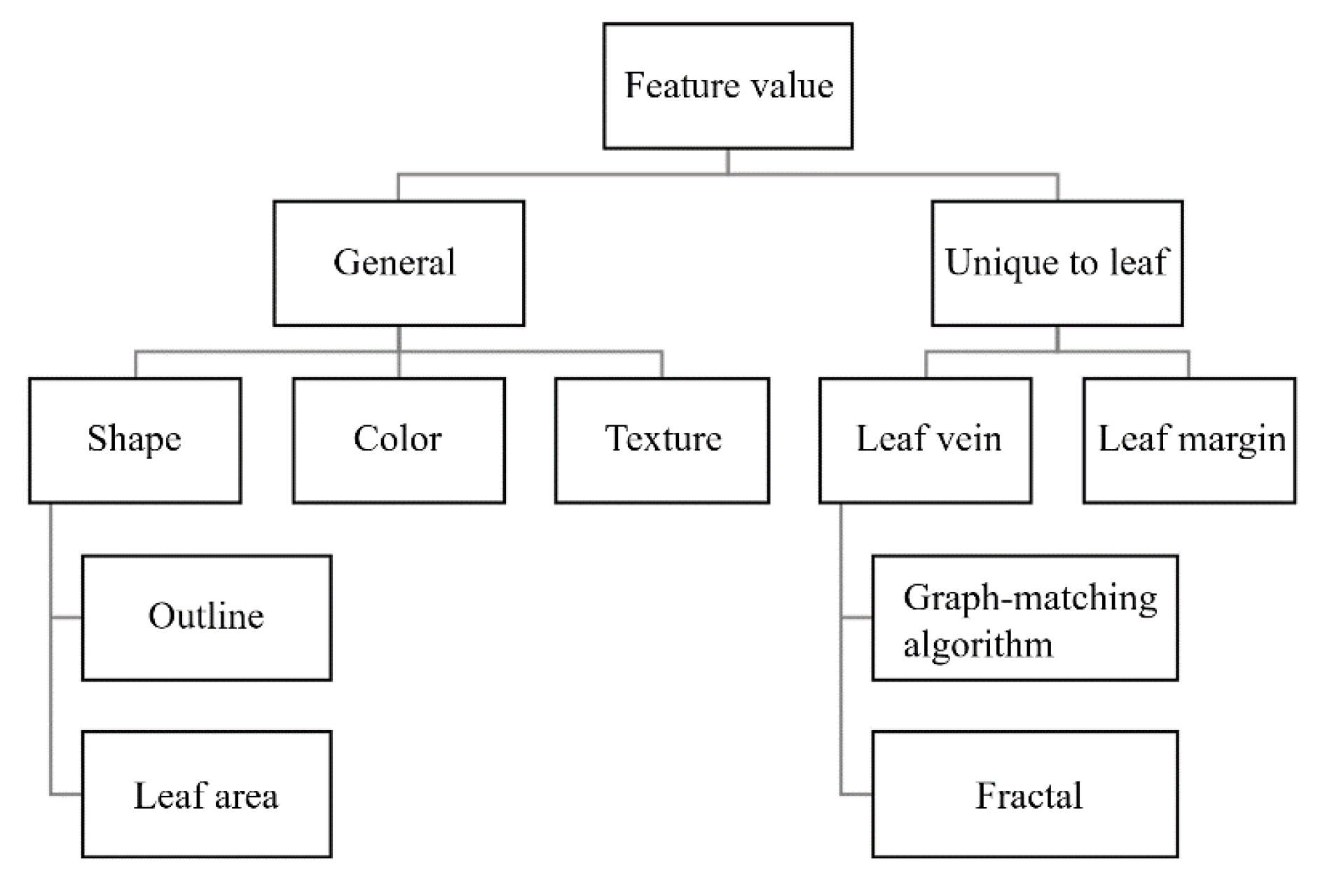
On the other hand, leaves are readily available as information because they can be easily collected year-round from almost any plant, including fossils and rare plants. Furthermore, leaf structures are planar, making them easy to collect, store, and image. Because these aspects simplify the data collection process, leaf morphology is the most studied feature in plant identification [6,14]. Figure 1 shows the main leaf features and their descriptors proposed for the automatic classification of plant species.

Leaf characteristics can be divided into two main categories: general characteristics such as shape, color, and texture, and characteristic quantities specific to leaves such as veins and leaf margins. Of these properties, shape is the one that has been studied most extensively [14]. Research on automatic shape classification can be divided into two main categories: methods that quantify the outline of the leaf and methods that quantify the leaf region (area, axial length, etc.). While shape characteristics are simple and readily available and therefore easy to use as information, they often vary considerably even among leaves of the same species, making automatic classification by shape alone difficult. Therefore, shape features are usually used in combination with other features.

For color features, descriptors such as color moments (CM), color histograms (CH), color coherence spectra, and color correlograms have been proposed [15]. The main challenge in describing color characteristics is that there are considerable differences due to the intensity and angle of the light at the time of capture, as well as different color temperatures [14]. In addition, Yanikoglu et al [16] reported that color information does not contribute at all to classification accuracy when combined with shape and texture descriptors. For these reasons, there are few studies on color characteristics.

For texture features, the main descriptors proposed are the Gabor filter (GF), fractal dimension (FD), and gray-level co-occurrence matrix (GLCM). GF has been widely employed to extract texture features from images, and Casanova et al [17] applied GF to textured images without leaf margin and reported higher accuracy than traditional texture analysis methods such as FD and GLCM. On the other hand, some literature claims that fractal analysis is the most suitable method for texture analysis because objects in nature [18], such as the surface of a leaf, have random and persistent patterns [19]. Jarbas et al [20] proposed a method that combines FD and lacunarity in a gravity model and found it to be superior to GF, FD, and GLCM. None of the texture analysis methods rely on complete leaf shape, as they can classify plants based on only one part of the leaf. Thus, it is very useful for the purpose of identifying plants that have been damaged by insect bites or other problems.

The leaf veins and leaf margins are characteristic quantities that are unique to the leaf. Since hand vein patterns are used in ecological authentication [21], leaf vein features can be a powerful source of information in plant identification. Larese et al [22] calculated 52 measurements (total number of edges, total number of nodes, network length, vein length, etc.) from the veins and examined the measurements needed for automatic identification. Nam et al [23] reported applying a graph matching algorithm called Venation Matching (VM) to leaf veins and combining it with shape features to obtain high accuracy. Bruno et al [12] applied Minkowski's multiscale fractal dimension method (Multiscale Minkowski-Sausage) to images of leaf outlines and veins to attempt automatic recognition, and reported a high recognition rate when the two methods were combined.

Bruno et al [12] proposed an automatic plant identification method based on multiscale fractal dimension. The resulting average misclassification rate of 2.5% is good, indicating that multi-scaling fractal analysis is a useful method for feature extraction in leaf veins.

Bruno et al. extracted and analyzed only the central and lateral veins of the leaf veins and did not deal with information on the fine veins. In light of the aforementioned ecological authentication technology, it would be possible to improve accuracy by also analyzing veinlets. In fact, Wilf et al [13] obtained excellent results in family and order classification by machine learning of vein images and leaf shape images, including veinlets.

However, Minkowski's multi-scaling fractal analysis used in this method uses the extrema of the resulting graph as features and does not interpret the features semantically. In contrast, in the other means of obtaining fractal dimension, called multifractal analysis, which extends the Hausdorff-Besicovitch dimension, the features obtained are values related to shape, entropy, etc. Leaf features can be used not only for plant identification, but also as indicators for other basic research, such as the study of potential leaf diseases. In the future, if breeding attempts are made to create disease-resistant plants based on these values, features that can be associated with shape and entropy could be more informative than features that have no semantic interpretation. Minkowski's multiscaling fractal analysis is also based on the assumption that objects in nature are unlikely to be mathematically perfect fractals, and multifractal analysis is based on the same assumption. Since multi-scaling fractal analysis is useful as a feature extraction method for leaf veins, we believe that multi-fractal analysis is also useful as a feature extraction method for leaf veins.

For these reasons, we propose a method of applying multifractal analysis to images of leaf veins, including veinlets.

2. Materials and Methods

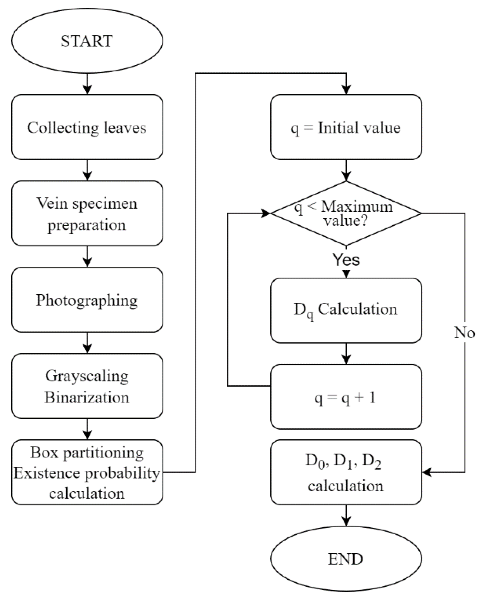
In this study, we propose a method to apply the capacity dimension, information dimension, and correlation dimension resulting from multifractal analysis to leaf veins. These values will be used to allow quantitative evaluation of the characteristics of the leaf veins. A flowchart of the proposed method is shown in Figure 2.

2.1. Preparation of Leaf Vein Specimens

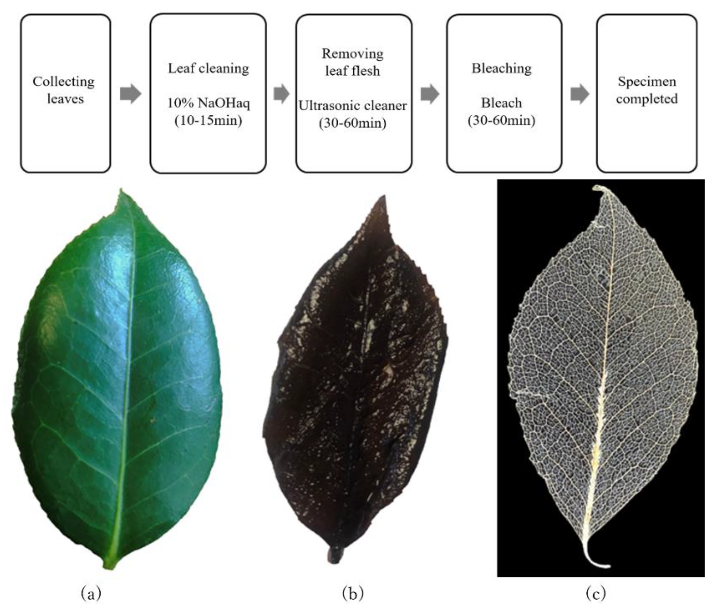
The contrast of leaf veins captured with a normal camera is very low, as shown in Figure 3(a), and it is difficult to extract only the leaf veins from this image. Therefore, the leaves are first washed with chemicals to remove the leaf flesh, and only the leaf veins are extracted to prepare leaf vein specimens. The procedure for preparing leaf vein specimens is shown in Figure 3.

First, a 10% sodium hydroxide solution is prepared and brought to a boil, then the leaves to be used for analysis are added and heated for 10-15 minutes. The condition of the leaves after heating for 10-15 minutes is shown in Figure 3(b). The leaves are then neutralized by feeding them into acid, and the leaf flesh is removed in an ultrasonic cleaner to obtain leaf vein specimens. The specimens obtained here are brown in color, but for the convenience of future photography and image processing, the leaf veins were removed by soaking in bleach for 30 minutes to 1 hour to remove the color of the veins to produce white to pale yellow specimens. The completed leaf vein specimen is shown in Figure 3(c).

2.2. Photographing and Pretreatment of Specimens

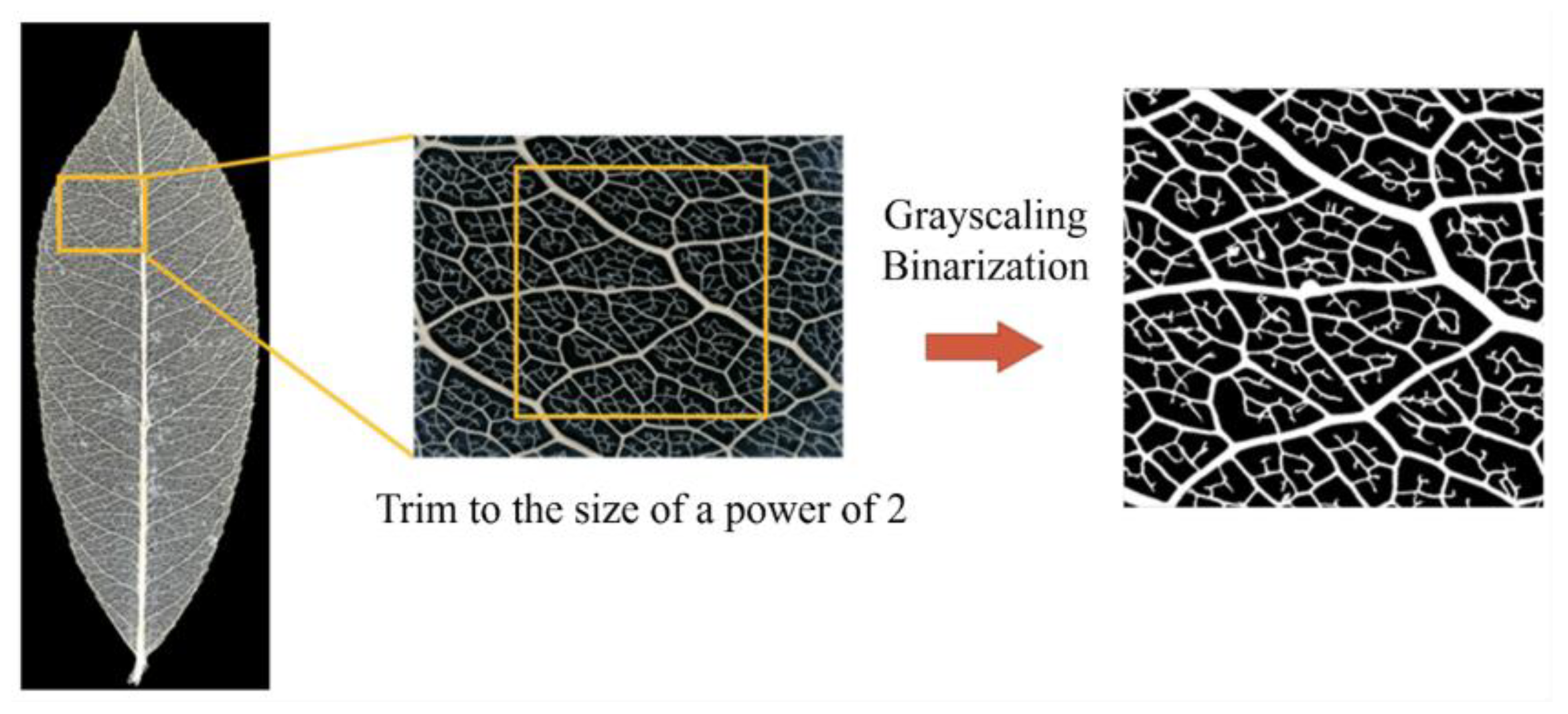
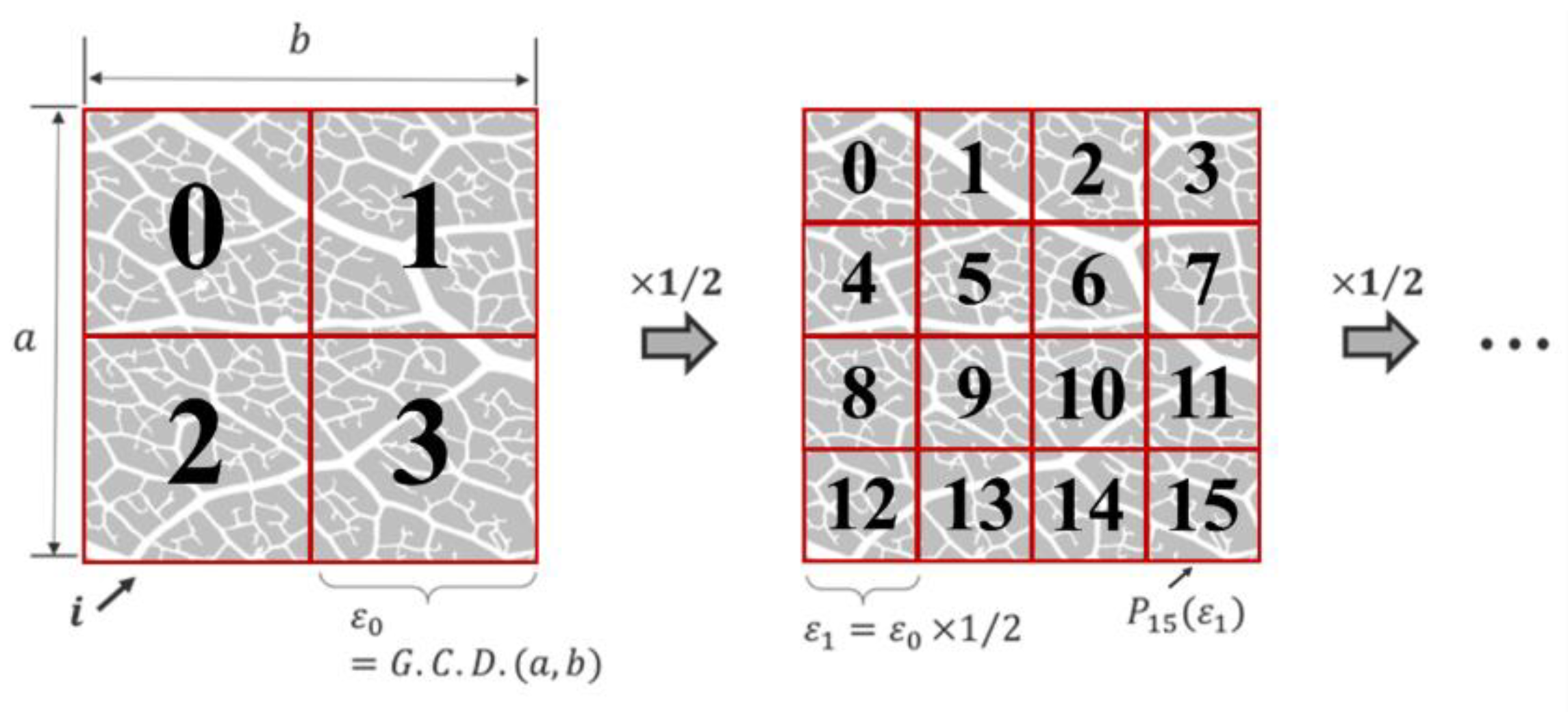
Next, the specimens prepared in 2.1 are photographed against a black background. The use of an electron microscope to capture images clearly shows veinlets. The captured image data is then preprocessed so that it can be analyzed for multifractal analysis. The pretreatment procedure is shown in Figure 4. First, the image is grayscaled, binarized, and morphologically transformed to create an image from which only the leaf veins are extracted. Multifractal analysis repeats the process of multiplying the width of the boxes that divide the image by 1/2, as shown in Figure 5, so the image size should be a power of 2. Therefore, trim the image to an appropriate size.

2.3. Box Partitioning and Existence Probability Calculation

The image is divided into boxes as shown in Figure 5, and the existence probability of each box,

P_{i} (ε)

, is obtained from Equation (1).

P_{i} (ε) = \frac{N_{i}}{N}

(1)

where ε is the box size, i is the box number, N is the total number of white pixels in the entire image, and

N_{i}

is the number of white pixels in the i-th box. The specified value of the box size ε was experimentally set as the value at which all leaves used in the experiment exhibit multifractality in dimensions 0, 1, and 2, with a maximum value of 2048 [pixels] and a minimum value of 8 [pixels]. Then repeat ε = ε x 1/2 until ε = 2048 to ε = 8. For each ε, we store the existence probability

P_{i} (ε)

, which is the percentage of the total number of white pixels (= pixels with a luminance value of 255) in the i-th box.

2.4. Calculation of Fractal Generalized Dimensions

Using the values of

P_{i} (ε)

calculated in Section 2.3, determine

D_{q}

, f(α), and α(q).

D_{q}

is obtained from equations (2) and (3), α(q) from equation (4), and f(α) from equation (5). The

μ_{i} (ε)

used to calculate α(q) and f(α) is obtained in Equation (6).

D_{q} = \frac{1}{q - 1} \lim_{ε \to 0} \frac{\log \sum_{i = 1}^{N (ε)} P_{i} {(ε)}^{q}}{\log ε} (q \neq 1)

(2)

D_{1} = \lim_{ε \to 0} \frac{\sum_{i = 1}^{N (ε)} P_{i} (ε) \log P_{i} (ε)}{\log ε} (q = 1)

(3)

α (q) = \lim_{ε \to 0} \frac{\sum_{i = 1}^{N (ε)} μ_{i} (ε) \log P_{i} (ε)}{\log ε}

(4)

f (α) = \lim_{ε \to 0} \frac{\sum_{i = 1}^{N (ε)} μ_{i} (ε) \log μ_{i} (ε)}{\log ε}

(5)

μ_{i} (ε) = \frac{{P_{i} (ε)}^{q}}{\sum_{i = 1}^{N (ε)} P_{i} {(ε)}^{q}}

(6)

where q is the moment order.

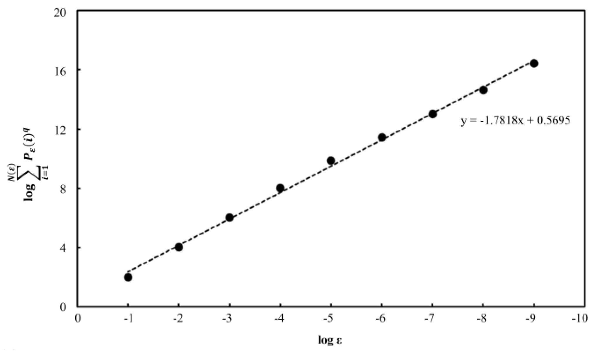
Equations (2)-(5) include the computation of limits in the equations. However, it is not possible to calculate the limits programmatically. Therefore, in this study, as shown in Figure 6, the values of the numerator and denominator of the equation were set to (x, y), and the slope obtained by linear regression was used as the result of the limit calculation. In this study, the least squares method was used for the linear regression technique.

The above process is performed over the specified q range to obtain

D_{0}

D_{1}

, and

D_{2}

from the

D_{q}

spectrum.

3. Results and Discussion

Two experiments were conducted to examine the usefulness of the method proposed in this study.

The first is to check whether the number of dimensions varies with the degree of leaf growth. This is necessary to know in advance the effect of the degree of growth on the leaf veins of the plant in order to realize automatic identification in the future.

The second is to check how the number of dimensions varies among the different taxonomic groups. With these results, it can be discussed whether automatic identification is possible with the proposed method in the future.

3.1. Experimant Environment

Table 1 shows the camera used to obtain the leaf area, Table 2 shows the specifications of the computer used for the analysis, and Table 3 shows the specifications of the electron microscope used during the imaging. In all leaves, the camera used during leaf area measurements was used to take pictures with the zoom set to equal magnification, and the electron microscope was used to take pictures with a magnification of 30x and a resolution of 12M.

Camera used

Ultra-wide-angle camera

3.2. Experiment 1: Verification Experiment of the Relationship between the Degree of Leaf Growth and the Number of Dimensions

3.2.1. Experiment Summary

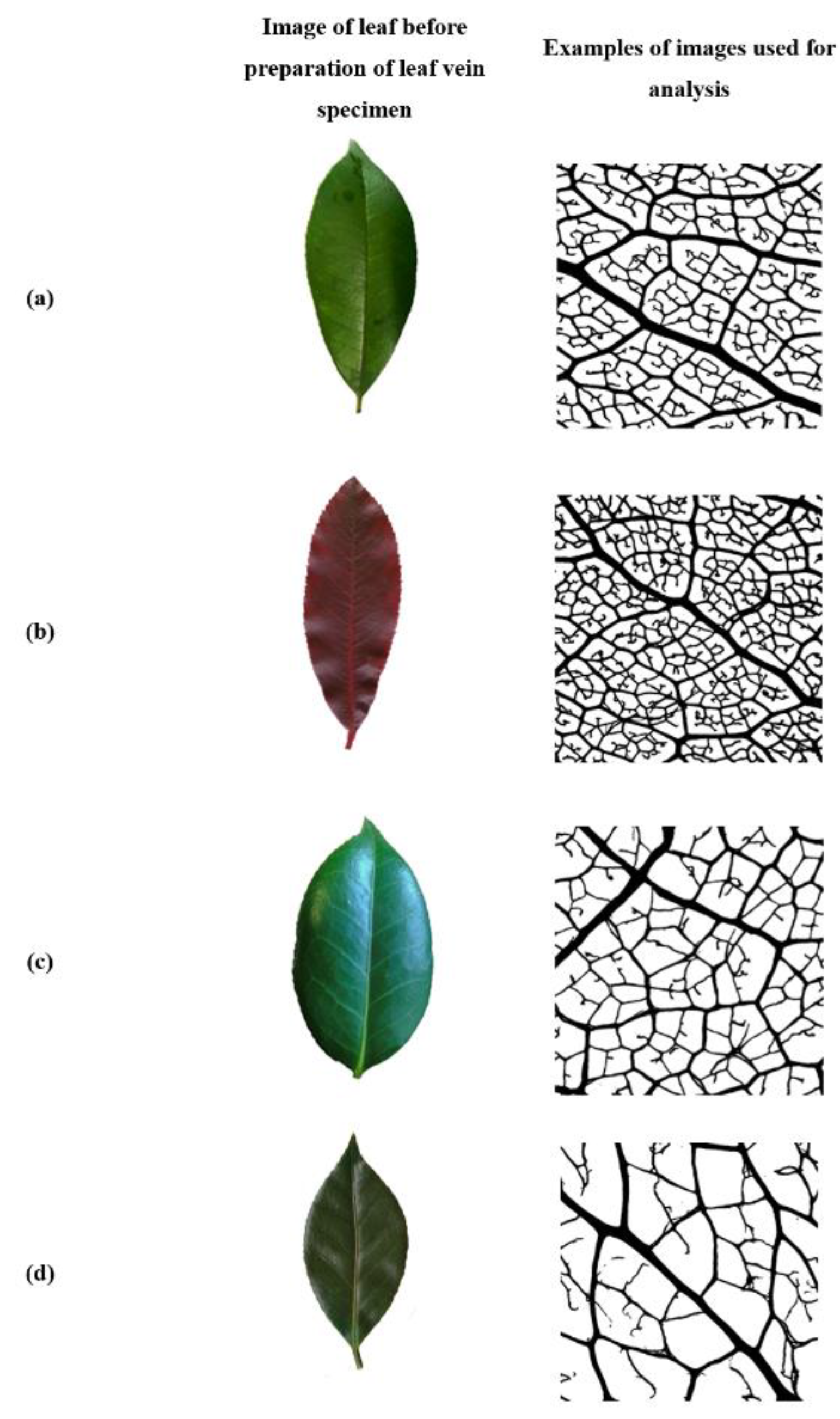
In Experiment 1, we used four species of trees that are known to be easy to prepare vein specimens: (a) Japanese photinia, (b) red tip, (c) Japanese hawthorn, and (d) common camellia. An example of a sample of each of the four plant species used in Experiment 1 is shown in Figure 7.

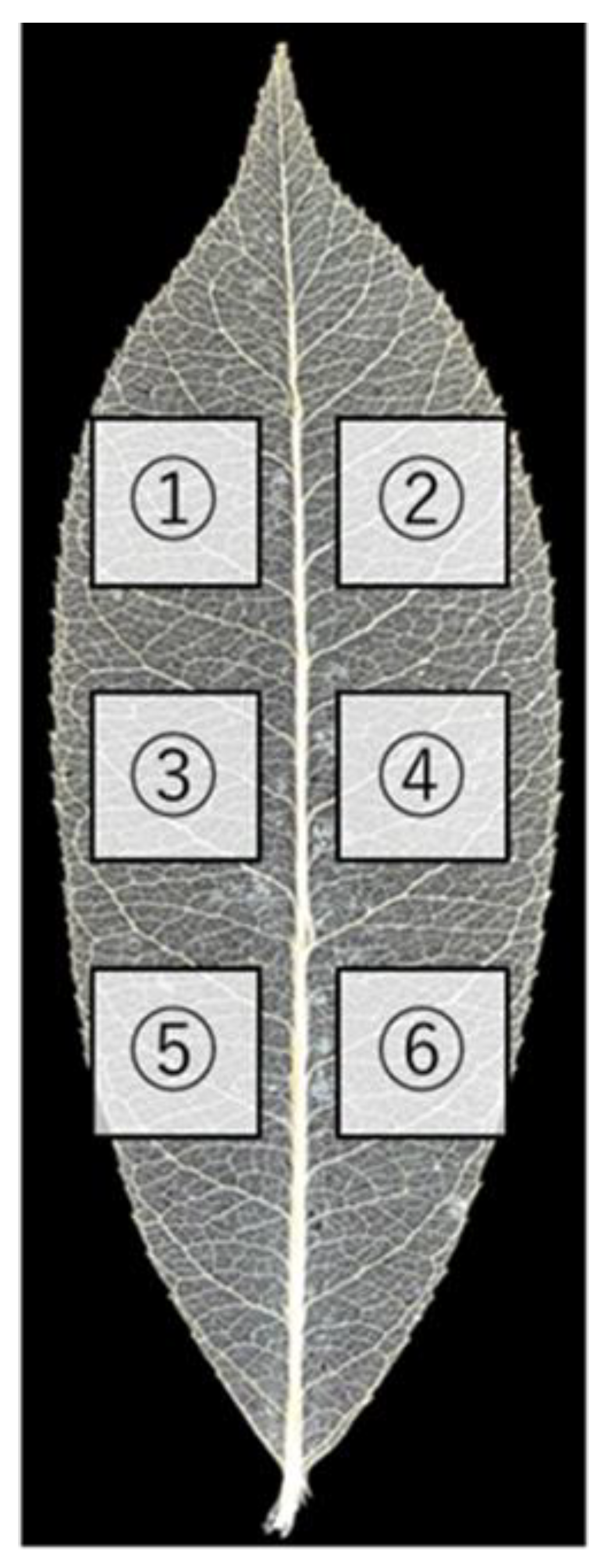
(a) was collected next to the smoking area in front of the old No. 10 building at the Setagaya Campus of Tokyo City University; (b) was collected from the hedge of the Denen Mansion Todoroki in Todoroki 2-chome, Setagaya-ku, Tokyo; (c) was collected at the entrance to the parking lot of Todoroki Valley in Setagaya-ku, Tokyo; and (d) was collected along the Kasai Water Oyasui (waterway) in Towa 2-chome, Adachi-ku, Tokyo. The position of the leaves to be collected was chosen so that they were evenly distributed from the base of the tree to the tip of the tree to avoid bias. Because only a portion of the leaf can be photographed at one time due to the convenience of using an electron microscope, six locations were photographed per sample: (1) upper left, (2) upper right, (3) left center, (4) center right, (5) lower left, and (6) lower right. The sample shooting positions are shown in Figure 8.

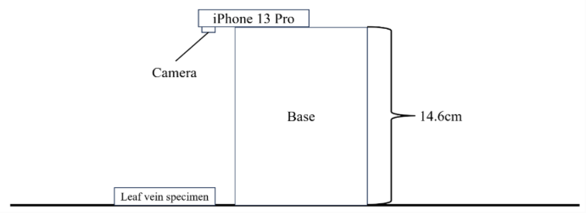
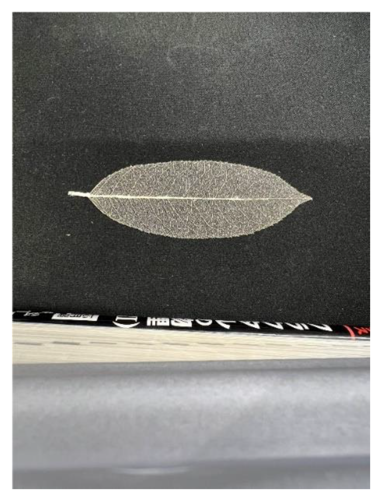
Because of the disorderly spread of tree branches, it is difficult to estimate the degree of leaf growth from their position. Therefore, the leaf area A of each leaf was determined, and the higher the value of A, the more mature the leaf. Leaf area A is a value used by Caglayan et al [24] as one of the leaf shape features and is the number of leaf pixels in the leaf area. In this study, leaves were photographed under similar photographic conditions, and the value of A was obtained by counting the total number of pixels in the leaf area. To photograph the leaves, a 14.6 cm base was made and the iPhone 13 Pro was placed so that the camera protrudes from the base toward the surface on which the leaves were placed. The angle between the base and the surface on which the leaves were placed was confirmed to be 0° with the iPhone's standard built-in measuring device. A schematic diagram of leaf photography is shown in Figure 9 and an example of an actual photograph is shown in Figure 10. After photographing, the images were pre-processed using CLIP STUDIO PAINT. The procedure is as follows

binarization at threshold 200.
gamut selection for white pixels.
Expand the selection by 10px and contract by 8px using the expansion type with rounded corners.
Fill in the selected area with white.
Fill in any additional areas within the foliage that are left unpainted.
Eliminate noise around leaves.
Trim the selection to exclude the base of the leaf.
Select the gamut where the pixels are white again, and perform trimming in the selected area.

An example of an image processed by the above procedure is shown in Figure 11. The value of A was obtained by counting the total number of white pixels in Figure 11.

3.2.2. Experimental Results

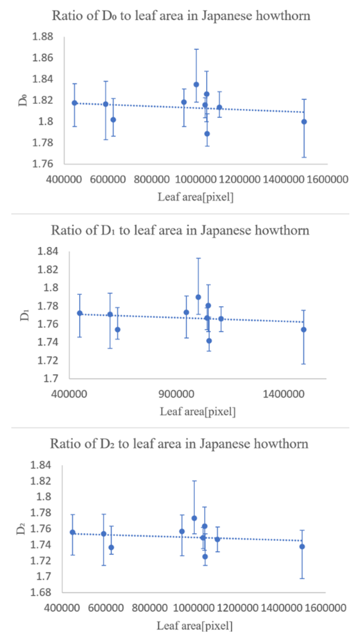
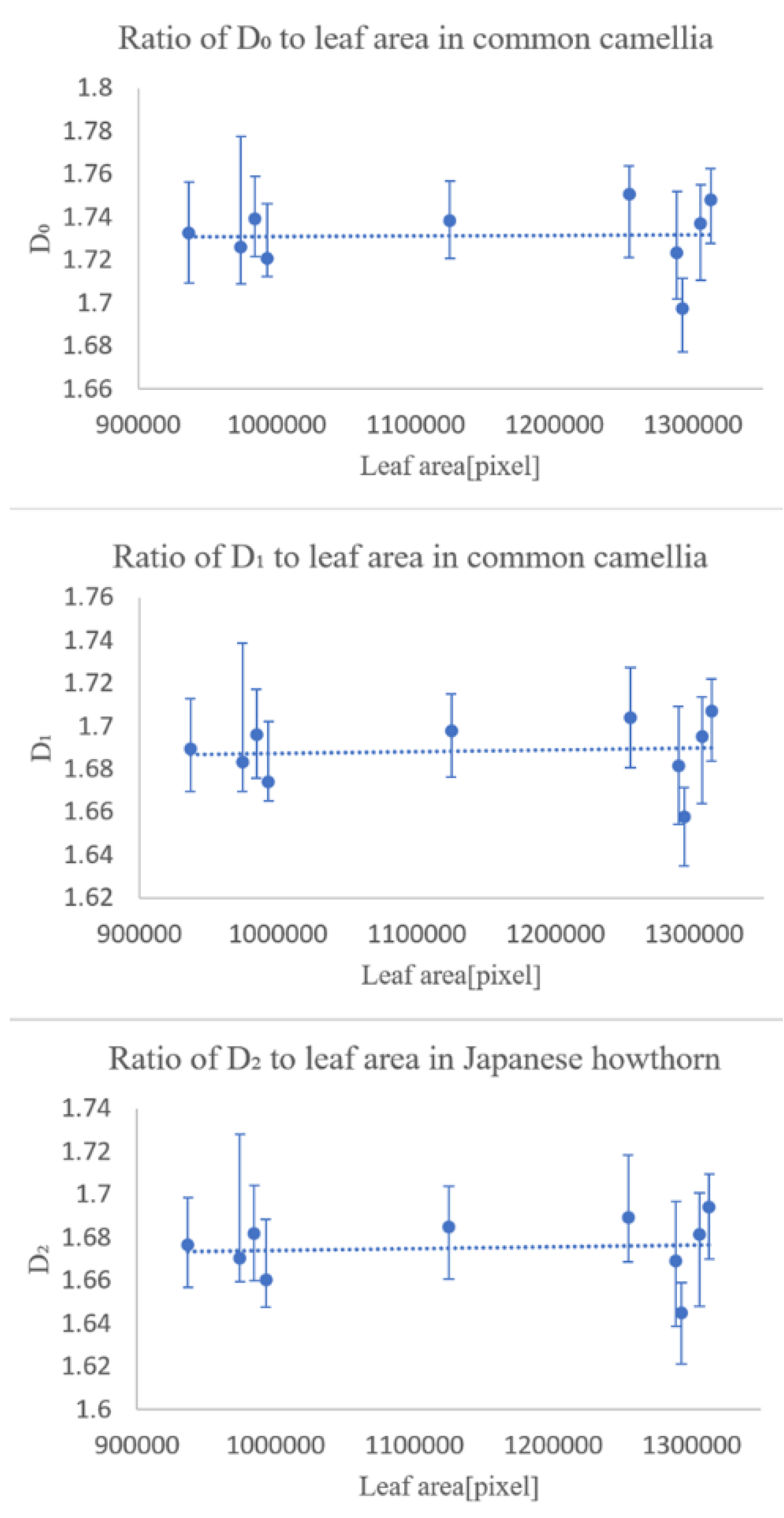
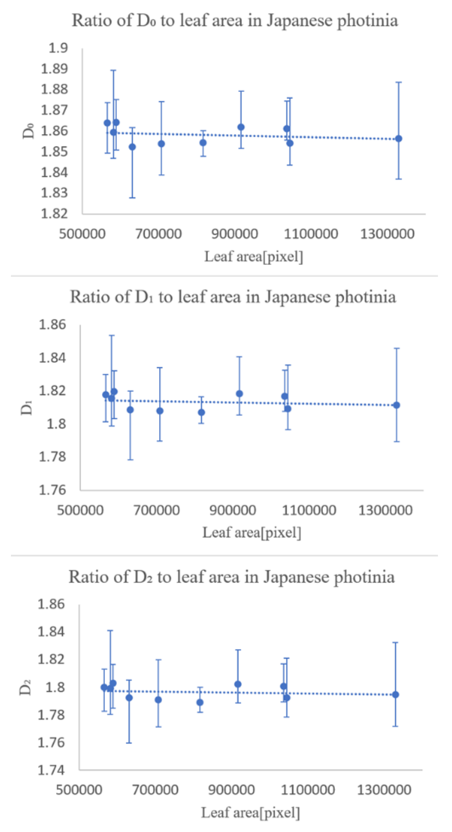
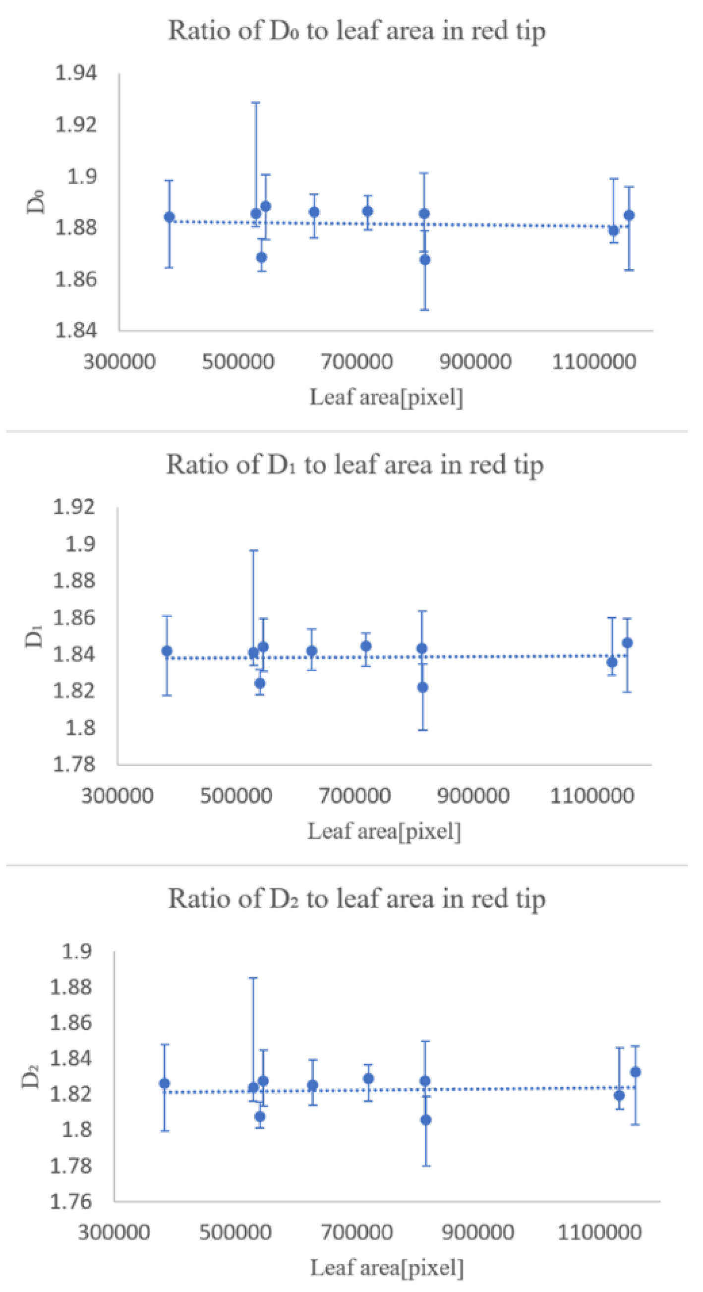
Figures 12 through 15 show the relationship between leaf area and the trimmed mean excluding the maximum and minimum of

D_{0}

D_{1}

, and

D_{2}

for the 10 samples. The dashed lines in the figure indicate the linear approximation by linear regression, and the error bars indicate the standard deviation of each sample, i.e., the variation of the analysis results for the shooting positions (1) to (6).

Figure 12. (a) Relationship between leaf area and fractal dimension values.

Figure 13. (b) Relationship between leaf area and fractal dimension values.

Figure 14. (c) Relationship between leaf area and fractal dimension values.

Figure 15. (d) Relationship between leaf area and fractal dimension values.

The coefficient of determination

R^{2}

for the linear approximation in (a) was 0.0499 for

D_{0}

, 0.039 for

D_{1}

, and 0.0268 for

D_{2}

. The slopes of the approximate curves were

{- 4.0 \times 10}^{- 9}

for

D_{0}

{- 4.0 \times 10}^{- 9}

for

D_{1}

, and

{- 3.0 \times 10}^{- 9}

for

D_{2}

The coefficient of determination

R^{2}

for the linear approximation in (b) was 0.0076 for

D_{0}

, 0.0016 for

D_{1}

, and 0.0093 for

D_{2}

. The slopes of the approximate curves were

{- 3.0 \times 10}^{- 9}

for

D_{0}

{- 1.0 \times 10}^{- 9}

for

D_{1}

, and

{- 3.0 \times 10}^{- 9}

for

D_{2}

The coefficient of determination

R^{2}

for the linear approximation in (c) was 0.0321 for

D_{0}

, 0.0332 for

D_{1}

, and 0.0353 for

D_{2}

. The slopes of the approximate curves were

{- 8.0 \times 10}^{- 9}

for

D_{0}

{- 8.0 \times 10}^{- 9}

for

D_{1}

, and

{- 9.0 \times 10}^{- 9}

for

D_{2}

The coefficient of determination

R^{2}

for the linear approximation in (d) was 0.0004 for

D_{0}

, 0.0068 for

D_{1}

, and 0.0082 for

D_{2}

. The slopes of the approximate curves were

{- 2.0 \times 10}^{- 9}

for

D_{0}

{- 8.0 \times 10}^{- 9}

for

D_{1}

, and

{- 8.0 \times 10}^{- 9}

for

D_{2}

3.2.3. Consideration

Based on the slope of the linear approximation and the value of the coefficient of determination, the values of the slope of the straight line in (a)-(d) are very small, and the value of the coefficient of determination is also very small, suggesting that the standard deviation of each sample is more influential than the effect of the degree of leaf growth on the veins.

These results indicate that the degree of leaf growth has little effect on the dimensionality of the veins, and that the error due to the location of the shot within the same sample is larger than the change due to the degree of growth.

3.3. Experiment 2: Experiments to Verify the Relationship between Taxonomy Group and Number of Dimensions

3.3.1. Experiment Summary

In Experiment 2, we used exactly the same image data as used in Experiment 1. The plant taxa used in Experiment 2 are listed in Table 4.

The purpose of Experiment 2 is to test the relationship between taxonomy group and number of dimensions. Therefore, we decided to verify the following four conditions.

(I) Verification of whether there is a difference in results between members of the same family and genus that differ only in species.

　(Comparison of (a) and (b), which are in the same family, Rosaceae, genus Photinia)

(II) Verification of whether there is a difference in results between different genera in the same family.

　(Comparison of the genera (a,b) Photinia and (c) Rhaphiolepis, which are in the same family, Rosaceae)

(III) Verification of whether there is a difference in results between different families.

　(Compare (a,b,c) Rosaceae and (d) Camellia, which are also in the same family)

(IV) Verification of whether there is a difference in results between different species.

　((a)-(d)) Comparison of each)

In this case, comparisons between two samples were verified using Welch's t-test as in Experiment 2, and comparisons between three or more samples were verified using Tukey's multiple comparisons.

3.3.2. Experimental Results (I) Comparison among Those Differing Only in Species

The null hypothesis is that fractal dimension classification is not possible for species that differ only in species, while the alternative hypothesis is that fractal dimension classification is possible for species that differ only in species. The results of Welch's t-test (significance level α=.05) are shown in Table 5.

3.3.3. Considerations (I) Comparison among Those Differing Only in Species

Welch's t-test results showed significant differences between conditions (a) and (b) for all values of

D_{0}

D_{1}

, and

D_{2}

. As a result, the null hypothesis is rejected, and we can infer that the results of

D_{0}

D_{1}

, and

D_{2}

are fractal dimension classification is possible for species that differ only in species.

3.3.4. Experimental Results (II) Comparison between Different Genera in the Same Family

The null hypothesis is that fractal dimension classification is not possible for species that same family, differ genus, while the alternative hypothesis is that fractal dimension classification is possible for species that same family, differ genus. The results of Welch's t-test (significance level α=.05) are shown in Table 6.

3.3.5. Considerations (II) Comparison between Different Genera in the Same Family

Welch's t-test results showed significant differences between conditions (a, b) and (b) for all values of

D_{0}

D_{1}

, and

D_{2}

. As a result, the null hypothesis is rejected, and we can infer that the results of

D_{0}

D_{1}

, and

D_{2}

are fractal dimension classification is possible for species that same family, differ genus.

3.3.6. Experimental Results (III) Comparison between Different Families

The null hypothesis is that fractal dimension classification is not possible for species that differ family, while the alternative hypothesis is that fractal dimension classification is possible for species that differ family. The results of Welch's t-test (significance level α=.05) are shown in Table 7.

3.3.7. Considerations (III) Comparison between Different Families

Welch's t-test results showed significant differences between conditions (a, b) and (b) for all values of

D_{0}

D_{1}

, and

D_{2}

. As a result, the null hypothesis is rejected, and we can infer that the results of

D_{0}

D_{1}

, and

D_{2}

are fractal dimension classification is possible for species that same family, differ genus.

3.3.8. Experimental Results (IV) Comparison between Different Species

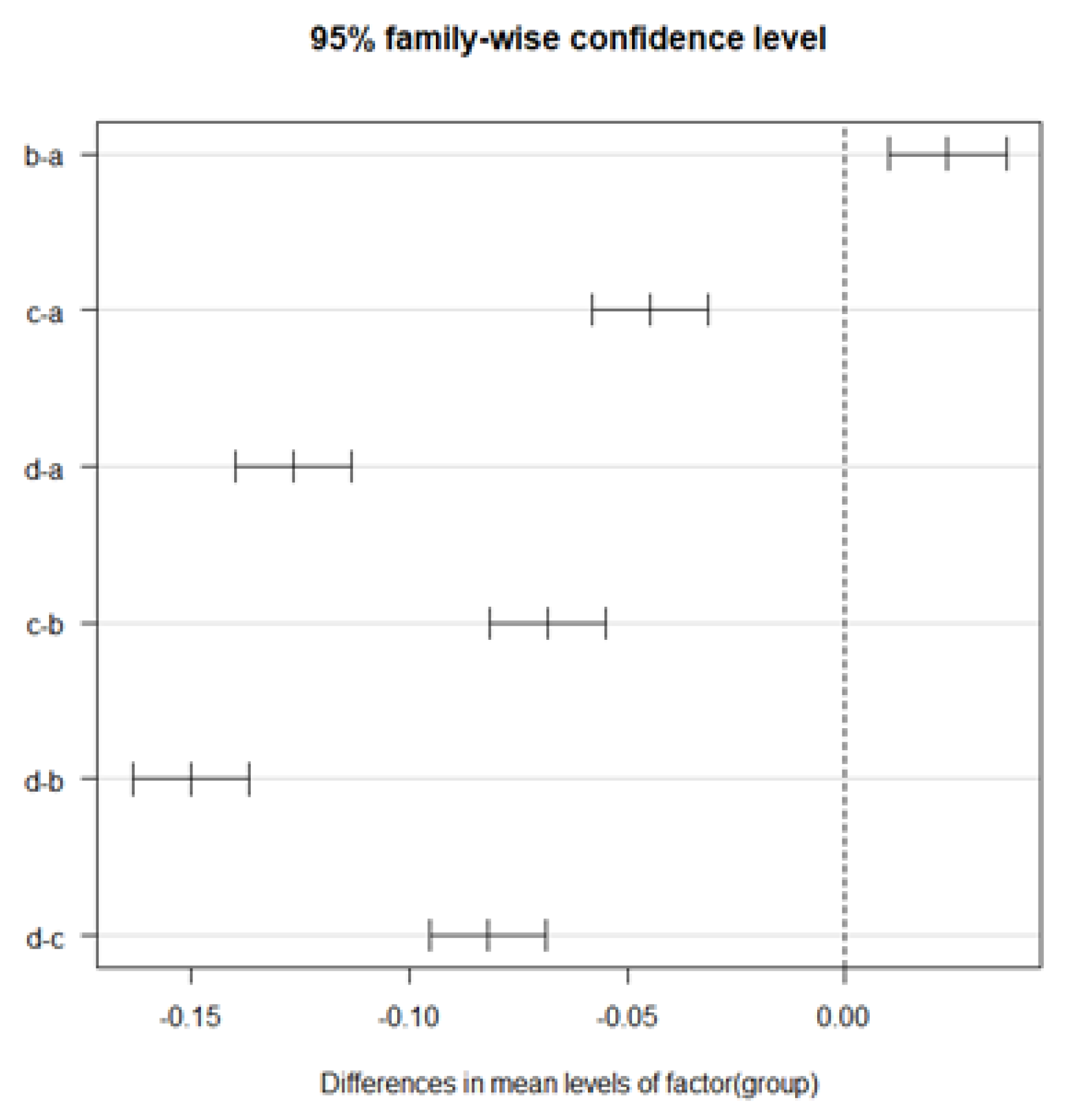
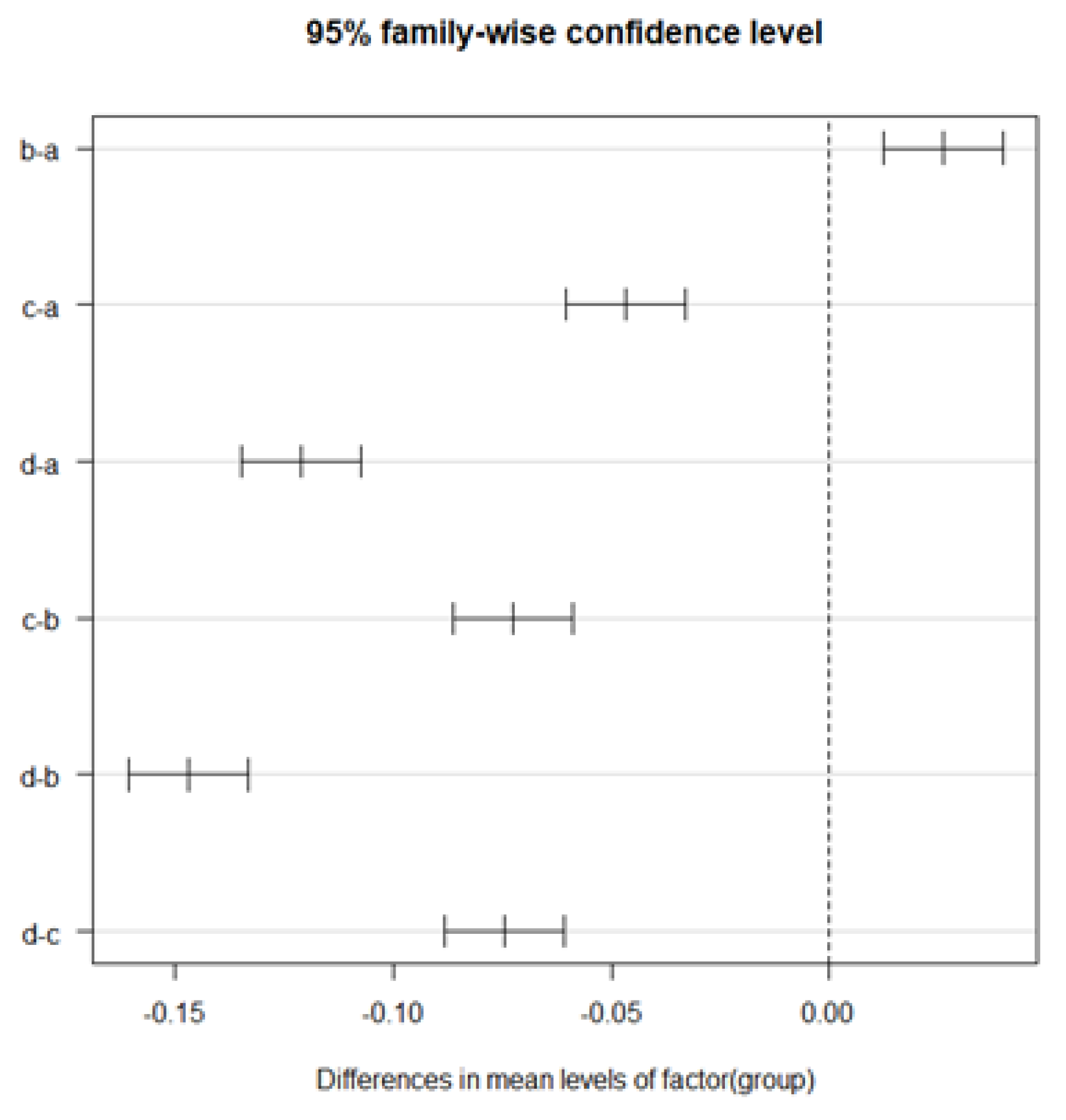
Since we wanted to test whether there were differences in the data among the four samples for comparisons between different species, we used analysis of variance rather than t-tests to make the comparisons. One-way ANOVA (significance level α=.05) was used for factors (a)-(d), since only one of the species information was available. Tables 8 through 10 show the results of one-way ANOVA for

D_{0}

D_{1}

, and

D_{2}

, respectively. As a result, significant differences between data groups were obtained for all

D_{0}

D_{1}

, and

D_{2}

. Therefore, we compared the differences between data groups by performing multiple comparisons. Tukey's multiple comparisons were used for multiple comparisons. The results of multiple comparisons (with a confidence interval of .95) for

D_{0}

D_{1}

, and

D_{2}

, respectively, are shown in Figure 16, Figure 17 and Figure 18. The results of multiple comparisons are shown as pairs of data on the vertical axis and confidence intervals on the horizontal axis.

Table 8. Results of one-way ANOVE (

D_{0}

Table 8. Results of one-way ANOVE (

D_{0}

Variable cause	Square sum	Degree of freedom	Average square	F	p
Column average	0.1313	3	0.0438	353.0	9.698 * 10⁻²⁷
Measurement error	0.0045	36	0.0001
Total	0.1358	39

Table 9. Results of one-way ANOVE (

D_{1}

Table 9. Results of one-way ANOVE (

D_{1}

Variable cause	Square sum	Degree of freedom	Average square	F	p
Column average	0.1302	3	0.0434	337.9	2.066 * 10⁻²⁶
Measurement error	0.0046	36	0.0001
Total	0.1348	39

Table 10. Results of one-way ANOVE (

D_{2}

Table 10. Results of one-way ANOVE (

D_{2}

Variable cause	Square sum	Degree of freedom	Average square	F	p
Column average	0.1249	3	0.0416	322.2	4.728 * 10⁻²⁶
Measurement error	0.0047	36	0.0001
Total	0.1296	39

3.3.9. Considerations (IV) Comparison between Different Species

From Figures 16 to 18, we can confirm that there are significant differences in all pairs for both

D_{0}

D_{1}

, and

D_{2}

. In other words, all data can be considered unrelated data.

Based on these results, it could be inferred that all combinations of different species could be classified when compared to each other. Therefore, the proposed method can extract features of leaf veins, suggesting the possibility of classifying plants into taxonomic groups from the results obtained by the proposed method.

4. Conclusions

In this study, we proposed a method for automatic plant identification by applying multifractal analysis to leaf vein images that include veinlets. Two experiments were conducted to verify the effectiveness of the proposed method.

In the first experiment, we checked whether the fractal dimensionality varied with the degree of leaf growth. The results showed that the degree of leaf growth had little effect on the fractal dimension number of the leaf veins.

The second experiment was conducted to see how the fractal dimensionality varied among the different classification groups, and the results suggested that classification was possible for all of same family and genus, differing only in species, same family, differing genus, differing family, and differing species.

The experimental results suggest that multifractal analysis can be applied to images of leaf veins, including veinlets, to enable automatic plant identification. However, we would like to collect more data in the future, because the magnitude of the effect of errors caused by the shooting position in the sample is unclear, and we have only been able to conduct experiments on four types of trees.

Author Contributions

Conceptualization, Y.S., Y.M. and Y.B.; methodology, Y.S. and Y.M.; software, Y.S.; validation, Y.S. and Y.B.; formal analysis, Y.S.; investigation, Y.S.; resources, Y.S., Y.M. and Y.B.; data curation, Y.S.; writing—original draft preparation, Y.S.; writing—review and editing, Y.S. and Y.B.; visualization, Y.S.; supervision, Y.B.; project administration, Y.B.; funding acquisition, Y.B. All authors have read and agreed to the published version of the manuscript.

Funding

This research received no external funding.

Institutional Review Board Statement

Not applicable.

Informed Consent Statement

Not applicable.

Data Availability Statement

The datasets used or analyzed during the current study are available from the corresponding author upon reasonable request.

Conflicts of Interest

We declare that there is no conflict of interest.

References

Antonelli, A.; Fry, C.; Smith, R.J.; Simmonds, M.S.J. State of the world’s plants and fungi 2020. Royal Botanic Gardens, KEW. [CrossRef]
Hagedorn, G.; Rambold, G.; Martellos, S.; Types of identification keys. Tools for Identifying Biodiversity: Progress and Problems 2010, 59-64. Available online: https://www.openstarts.units.it/server/api/core/bitstreams/d6c3dc5f-17a1-478b-beab-31464b220ce1/content (accessed on 3 October 2024).
Fransworth, E.J.; Chu, M.; Kress, W.J.; Neill, A.K.; Best, J.H.; Pickering, J.; Stevenson, R.D.; Courtney, G.W.; VanDyk, J.K.; Ellison, A.M. Next-Generation Field Guides. BioScience 2013, 11, 891–899. [Google Scholar] [CrossRef]
Frankilin, J. Mapping Species Distributions: Spatial Inference and Prediction. Cambridge University Press 2010. [CrossRef]
Hopkins, G.W.; Freckleton, R.P. Declines in the numbers of amateur and professional taxonomists: implications for conservation. Animal Conservation 2002, 3, 245–249. [Google Scholar] [CrossRef]
Wäldchen, J.; Rzanny, M.; Seeland, M.; Mäder, P. Automated plant species identification—Trends and future directions. PLoS Computational Biology 2018. [CrossRef] [PubMed]
Karimata, T.; Oono, H.; Osa, A.; Miike, H.; A Study on Feature Extraction from Leaf Vein Image Using Fractal Image Analysis. Bulletin of the Society for Science on Form 2008, 23, 2, 218-219. Available online: https://cir.nii.ac.jp/crid/1572543025608664448 (accessed on 3 October 2024).
Kido, Y.; Takeuchi, M.; Matsuda, O.; Moriguchi, J.; Yamane, W.; Maeda, N.; Mandai, I.; Akihiro, T. Establishment of iPis, a web-based system for identifying plant species using leaf and branch traits as the primary identification criteria. The Japanese Society for Plant Systematics 2016, 1, 63–71. [Google Scholar] [CrossRef]
Gaston, K.J.; O’Neill, M.A. Automated species identification: why not? Philos Trans R Soc Lond B Biol Sci 2004, 1444, 655–667. [Google Scholar] [CrossRef] [PubMed]
Saitoh, T.; Kaneko, T.; Automatic Recognition of Flower Images Based on Natural Images. The IEICE Transactions on Information and Systems D 2005, J88-D2, 12, 2341-2349. Available online: https://search.ieice.org/bin/summary.php?id=j88-d2_12_2341&category=D&lang=J&year=2005&abst= (accessed on 3 October 2024).
Shindo, T.; Yang, L-L. ; Hoshino, Y.; Cao, Y. A Fundamental Study on Plant Classification Using Image Recognition by AI. The 61st Automatic Control Union Lecture Meeting 2018, 175–179. [Google Scholar] [CrossRef]
Bruno, O.M.; Plotze, R. de O.; Falvo, M.; Castro, M. Fractal dimension applied to plant identification. Information Sciences 2008, 12, 2722–2733. [Google Scholar] [CrossRef]
Wilf, P.; Zhang, S.; Chikkerur, S.; Little, S.A.; Wing, S.L.; Serre, T. Computer vision cracks the leaf code. PNAS, 3305; 12. [Google Scholar] [CrossRef]
Wäldchen, J.; Mäder, P. Plant Species Identification Using Computer Vision Techniques: A Systematic Literature Review. Arch Computat Methods Eng 2018, 2, 507–543. [Google Scholar] [CrossRef] [PubMed]
Zhang, D.; Islam, M.M.; Lu, G. A review on automatic image annotation techniques. Pattern Recognition 2012, 1, 346–362. [Google Scholar] [CrossRef]
Yanikoglu, B.A.; Aptoula, E.; Tirkaz, C. Automatic plant identification from photographs. Machine Vision and Applications 2014, 6, 1369–1383. [Google Scholar] [CrossRef]
Casanova, D.; Sá Junior, J.J. de M.; Bruno, O.M. Plant Leaf Identification Using Gabor Wavelets. International Journal of Imaging Systems and Technology 2009, 3, 236–243. [Google Scholar] [CrossRef]
Huang, P.W.; Dai, S.K.; Lin, P.L. Texture image retrieval and image segmentation using composite sub-band gradient vectors. Journal of Visual Communication and Image Representation 2006, 5, 947–957. [Google Scholar] [CrossRef]
Backes, A.R.; Bruno, O.M. Fractal and Multi-Scale Fractal Dimension analysis: A comparative study of Bouligand-Minkowski method. arXiv:1201.3153v1, arXiv:1201.3153v1 2013, 7, 74-83. [CrossRef]
Sá Junior, J.J. de M.; Backes, A.R.; Cortez, P.C. Gravitational Based Texture Roughness for Plant Leaf Identification. International Conference on Computer Analysis of Images and Patterns 2013, 416–423. [Google Scholar] [CrossRef]
Rajalakshmi, M.; Rengaraj, R.; Charadwaj, M.; Kumar, A.; Raju, N.N.; Haris, M. An Ensemble Based hand Vein Pattern Authentication System. CMES 2018, 2, 209–220. [Google Scholar] [CrossRef]
Larase, M.G.; Bayá, A.E.; Craviotto, R.M.; Arango, M.R.; Gallo, C.; Granitto, P.M. Multiscale recognition of legume varieties based on leaf venation images. Expert Systems with Applications 2014, 10, 4638–4647. [Google Scholar] [CrossRef]
Nam, Y.; Hwang, E.; Kim, D. CLOVER: A Mobile Content-Based Leaf Image Retrieval System. International Conference on Asian Digital Libraries 2005, 139–148. [Google Scholar] [CrossRef]
Caglayan, A.; Guclu, O.; Can, A.B. A Plant Recognition Approach Using Shape and Color Features in Leaf Images. ICIAP 2013 2013, 161–170. [Google Scholar] [CrossRef]

Figure 1. Main leaf features and their descriptors used for automatic classification [14].

Figure 2. Procedures.

Figure 3. Procedures for preparing leaf vein specimens.

Figure 4. Shooting and pre-processing procedures.

Figure 5. Box split.

Figure 6. Calculate the extreme values of

D_{q}

(the extreme values of f(α) and α(q) are obtained in the same way).

Figure 6. Calculate the extreme values of

D_{q}

(the extreme values of f(α) and α(q) are obtained in the same way).

Figure 7. An example of a sample used in the experiment.

Figure 8. Sample shooting positions (1) to (6).

Figure 9. Schematic diagram of leaf photography.

Figure 10. Examples of actual photo.

Figure 11. Examples of processed image.

Figure 16. Results of Tukey’s multiple comparisons in

D_{0}

Figure 16. Results of Tukey’s multiple comparisons in

D_{0}

Figure 17. Results of Tukey’s multiple comparisons in

D_{1}

Figure 17. Results of Tukey’s multiple comparisons in

D_{1}

Figure 18. Results of Tukey’s multiple comparisons in

D_{2}

Figure 18. Results of Tukey’s multiple comparisons in

D_{2}

Table 1. Camera used.

Model name	iPhone 13 Pro
Camera used	Ultra-wide-angle camera

Table 2. Computer specifications used.

OS	Windows 11 Home
CPU	Intel® Core™ i9-10900K / 3.70GHz
RAM	32GB

Table 3. Electron microscope specs used.

Sensor		5-megapixel CMOS sensor
Zoom magnification	Optical Zoom	10 – 300 times
Zoom magnification	Digital Zoom	Up to 4 times
Shooting resolution (still image)		12M, 9M, 5M, 3M, 1.3M, VGA
Format (still image)		JPEG

Table 4. Classification of plants used in Experiment 2.

Species	Technical name	Family	Genus
(a) Japanese photinia	Photinia glabra	Rosaceae	Photinia
(b) red tip	Photinia × fraseri ‘Red Robin’	Rosaceae	Photinia
(c) Japanese bowthorn	Rhaphiolepis umbellate	Rosaceae	Rhaphiolepis
(d) common camellia	Camellia japonica	Theaceae	Camellia

Table 5. Welch’s t-test results.

	$D_{0}$		$D_{1}$		$D_{2}$
	(a)	(b)	(a)	(b)	(a)	(b)
Average	1.858	1.882	1.813	1.839	1.797	1.823
Decentralization	$2.01 * 10^{- 5}$	$5.68 * 10^{- 5}$	$2.4 * 10^{- 5}$	$7.27 * 10^{- 5}$	$2.65 * 10^{- 5}$	$8.01 * 10^{- 5}$
Number of observations	10	10	10	10	10	10
Degree of freedom	15		14		14
t	-8.463		-8.157		-7.965
P(T<=t) both sides	$4.27 * 10^{- 7}$		$1.09 * 10^{- 6}$		$1.44 * 10^{- 6}$
t Boundary value Both sides	2.131		2.145		2.145

Table 6. Welch’s t-test results.

	$D_{0}$		$D_{1}$		$D_{2}$
	(a, b)	(c)	(a, b)	(c)	(a, b)	(c)
Average	1.870	1.813	1.826	1.767	1.810	1.750
Decentralization	$1.81 * 10^{- 4}$	$1.78 * 10^{- 4}$	$2.15 * 10^{- 4}$	$1.94 * 10^{- 4}$	$2.29 * 10^{- 4}$	$1.96 * 10^{- 4}$
Number of observations	20	10	20	10	20	10
Degree of freedom	18		19		19
t	10.90		10.75		10.71
P(T<=t) both sides	$2.35 * 10^{- 9}$		$1.63 * 10^{- 9}$		$1.74 * 10^{- 9}$
t Boundary value Both sides	2.101		2.093		2.093

Table 7. Welch’s t-test results.

	$D_{0}$		$D_{1}$		$D_{2}$
	(a, b, c)	(d)	(a, b, c)	(d)	(a, b, c)	(d)
Average	1.851	1.732	1.806	1.689	1.790	1.675
Decentralization	$9.08 * 10^{- 4}$	$2.41 * 10^{- 4}$	$1.00 * 10^{- 3}$	$2.23 * 10^{- 4}$	$1.03 * 10^{- 3}$	$2.14 * 10^{- 4}$
Number of observations	30	10	30	10	30	10
Degree of freedom	31		33		34
t	16.22		15.76		15.30
P(T<=t) both sides	$1.07 * 10^{- 16}$		$6.37 * 10^{- 17}$		$8.19 * 10^{- 17}$
t Boundary value Both sides	2.040		2.035		2.032

Disclaimer/Publisher’s Note: The statements, opinions and data contained in all publications are solely those of the individual author(s) and contributor(s) and not of MDPI and/or the editor(s). MDPI and/or the editor(s) disclaim responsibility for any injury to people or property resulting from any ideas, methods, instructions or products referred to in the content.

© 2024 by the authors. Licensee MDPI, Basel, Switzerland. This article is an open access article distributed under the terms and conditions of the Creative Commons Attribution (CC BY) license (http://creativecommons.org/licenses/by/4.0/).

Copyright: This open access article is published under a Creative Commons CC BY 4.0 license, which permit the free download, distribution, and reuse, provided that the author and preprint are cited in any reuse.

MDPI Initiatives

Important Links

Choose an area of interest and we will send you notifications of new preprints at your preferred frequency.

Disclaimer

Leaf Vein Analysis of Different Plant Species Using Multifractal Analysis

Abstract

1. Introduction

2. Materials and Methods

2.1. Preparation of Leaf Vein Specimens

2.2. Photographing and Pretreatment of Specimens

2.3. Box Partitioning and Existence Probability Calculation

2.4. Calculation of Fractal Generalized Dimensions

3. Results and Discussion

3.1. Experimant Environment

3.2. Experiment 1: Verification Experiment of the Relationship between the Degree of Leaf Growth and the Number of Dimensions

3.2.1. Experiment Summary

3.2.2. Experimental Results

3.2.3. Consideration

3.3. Experiment 2: Experiments to Verify the Relationship between Taxonomy Group and Number of Dimensions

3.3.1. Experiment Summary

3.3.2. Experimental Results (I) Comparison among Those Differing Only in Species

3.3.3. Considerations (I) Comparison among Those Differing Only in Species

3.3.4. Experimental Results (II) Comparison between Different Genera in the Same Family

3.3.5. Considerations (II) Comparison between Different Genera in the Same Family

3.3.6. Experimental Results (III) Comparison between Different Families

3.3.7. Considerations (III) Comparison between Different Families

3.3.8. Experimental Results (IV) Comparison between Different Species

3.3.9. Considerations (IV) Comparison between Different Species

4. Conclusions

Author Contributions

Funding

Institutional Review Board Statement

Informed Consent Statement

Data Availability Statement

Conflicts of Interest

References

MDPI Initiatives

Important Links

Subscribe