1. Introduction
In recent years, there has been a marked surge in the utilization of autonomous industrial robots across various sectors. As industries seek to enhance efficiency and productivity, the deployment of these robots has become increasingly prevalent. However, with this proliferation comes the imperative to ensure their safe operation, particularly in dynamic and complex environments where they interact with other robots and humans. Consequently, research endeavors delving into the navigation of autonomous mobile robots in such intricate settings have gained considerable traction. These studies are pivotal not only for optimizing operational efficacy but also for safeguarding the well-being of both human workers and robotic counterparts [
1,
2].
On unknown environments, a fundamental capability of autonomous mobile robots is Simultaneous Localization and Mapping (SLAM) [
3,
4]. Most of the SLAM algorithms have the assumption of a static environment [
4,
5,
6]. On the other hand, on known indoor industrial environments one might ask why would be interesting to perform SLAM. In order to answer this question we need to consider the concept of Line-less Mobile Assembly Systems (LMAS) on Future Assembly Systems. The LMAS integrates temporal and spatial decoupling of resources alongside modern strategies for mobilizing all pertinent resources in industrial assembly processes to increase productivity and sustainability [
7]. In such flexible and highly dynamic systems, where assets are reorganized in time, the complexity of the environment increases and it is important to maintain surveillance of every assets’ location in the production system. In this paper, we do not focus on the classic SLAM approach, where the goal is to obtain the global pose of the sensor while simultaneously construct the full map of the environment. In our case, we are interested in obtaining the pose of the movable objects on the scene and simultaneously predicting their occupancy in 2D. These information together, can be used both for navigation and filtering the sensor data, resulting in more precise global localization or more effective path planning.
Regarding the tasks of tracking and segmenting movable objects, including robots and humans, Convolutional Neural Networks (CNNs) have been highly used due to their ability of learning from vasts amount of data and increasing performance over time. Training CNNs requires an extensive and varied dataset of precise annotations, a process often laborious and costly when done manually. To mitigate this challenge, simulation-based data generation has surfaced as a prospective solution. This approach leverages synthetic data to train CNNs for tasks such as object detection and segmentation [
8,
9].
In this paper, we investigate the following research question: How can we leverage advanced deep learning techniques, synthetic data generation, and ROS2-based communication frameworks to develop a robust perception system for autonomous navigation in dynamic environments, specifically focusing on multi-object detection and segmentation using 3D LiDAR data? Our hypothesis is that by using the Birds-Eye-View (BEV) representation of 3D LiDAR data, it is possible to perform accurate and fast detection, tracking and building of a semantic 2D map of the environment on top of the static map. The main objective is to design and evaluate a CNN that allows multi-source data aggregation and generation of this map for wheeled mobile robots path-planning and navigation.
The remaining sections of this paper are organized as follows.
Section 2 provides an overview of various researches in related areas alongside their difference to our approach.
Section 3 presents the framework of our system in detail, including tools, designs and evaluation metrics.
Section 4 shows the experiments and results of our system.
Section 5 provides ablation studies and analyses of the results. Finally, a brief conclusion is given in
Section 6.
2. Related Work
[
3] presented an extensive review of former multiple-robot SLAM systems, pointing out different aspects of different systems, such as data communication, distribution, processing, and several challenges, as relative poses of robots, uncertainty, updating maps and poses, line-of-sight observations, closing loops, complexity, heterogeneous robots and sensors, synchronization and performance measure. In dynamic environments, the authors state that very few works have been done in the field by that time, and the ones cited relies on detection and tracking the dynamic objects or their features.
Another survey about path planning in dynamic environments is presented by [
1] and [
2] show a survey on robotic semantic navigation systems for indoor environments. In both these surveys, a key component of most systems relies on the ability to detect or segment objects in the environment.
The majority of current LiDAR-based SLAM systems primarily utilize geometric information to depict the environment and establish correlations between observations and the map. These systems perform effectively under the presumption that the environment remains predominantly static [
10]. [
11] introduced
SuMa++, a novel approach to construct semantic maps by a laser-based semantic segmentation of the point cloud. By leveraging semantic consistencies between scans and the map, their method filters out dynamic objects and incorporates higher-level constraints during the Iterative Closest Point (ICP) process. This enables the successful integration of semantic and geometric information solely from three-dimensional laser range scans, resulting in significantly improved accuracy in pose estimation compared to a purely geometric approach. More recently, a filter-based approach is proposed by [
12] called
Point-LIO, a LiDAR-inertial odometry that offers robustness and high-bandwidth capabilities, and the ability to estimate extremely aggressive robotic motions. The authors of
Point-LIO state that their point-by-point strategy could be explored in dynamic object detection systems on future works.
Regarding 3D object detection,
CenterPoint proposed by [
13], is a center-based framework for simultaneous 3D object detection and tracking utilizing LiDAR point-clouds. Their approach employs a conventional 3D point-cloud encoder coupled with a small number of convolutional layers in the head to generate a bird’s-eye-view heatmap and additional dense regression outputs. Detection involves straightforward local peak extraction with refinement, while tracking relies on closest-distance matching. Their approach achieved state-of-the-art performance on the
Waymo and
nuScenes benchmarks, and was inspired by [
14] and [
15]. More recently, [
16] conduct an empirical and comprehensive investigation into essential components of real-time object detectors, encompassing model architectures, label assignment, data augmentations, and optimization techniques. Additionally, they delve into minimal adaptations of a high-precision real-time object detector for real-time instance segmentation and detection of rotated objects, resulting in a new family of models called
RTMDet.
[
17] introduced transformers, and the use of self-attention mechanisms have found widespread use in natural language processing. [
18] adapted their concept with the development of Visual Transformers (ViT), and it has gained rapid momentum in computer vision research. Notably, architectures such as BEVFormer [
19], for 3D detection and map segmentation, and OccFormer [
20], for 3D semantic occupancy prediction, have emerged as prominent examples. However, despite their recent popularity, transformers also come with certain limitations. One notable drawback is their increased computational complexity compared to CNNs, which can lead to higher training and inference costs, especially for large-scale models. Additionally, transformers may require larger datasets to achieve optimal performance due to their reliance on self-attention mechanisms, potentially posing challenges in scenarios with limited data availability [
21,
22,
23]. Considering these factors, in the design of our system, we opted for CNNs due to their proven efficiency and effectiveness in handling real-time object detection and tracking tasks, particularly in resource-constrained environments.
With respect to CNNs and synthetic data on industrial robot applications, a very common explored use-case is the task of bin-picking or pick-and-place [
8,
9,
24,
25], the common practice to train models using images where objects are positioned randomly, occasionally occluded, or even upside-down. However, in our navigation scenario, where the aim is to track and segment mobile robots, humans, and other movable objects, including upside-down instances in the training data is not beneficial, because they do not accurately represent the typical operating environment. Also, by using geometric simulated LiDAR data with noise, we aim to minimize the gap from simulation domain to real-world domain.
3. Materials and Methods
Tools: As Simulation platform, the Gazebo Simulator is used due to it’s open source development, integrated annotation sensors and facilitated communication with ROS2 framework [
26,
27].
For dataset generation, we extended the work done in [
28] to include 3D object detection and semantic segmentation annotations in BEV 3D Lidar data. Using this automated dataset generation and 23 simulation models divided in 14 classes, we created the synthetic dataset containing a total of 10593 annotated LiDAR samples divided in training (75,52%), validation (5,93%) and test (18,9%) sets. The classes consist of person, 6 different mobile robots and 7 different movable objects, and we specified 0,5 meter for LiDAR height position, considering that it would be attached to one of the robots.
For CNN design, training and inference, the PyTorch library is used in this project. Full dataset link, ROS2 packages, jupyter notebooks and video results are maintained in [
29].
CNN design and training: BEV representations are usually encoded using height, intensity and density channels [
30]. On our specific use case, despite of LiDAR’s distance sensing range and 360 degrees horizontal field of view, we defined an area of 10x10 meters in front of the sensor to build a 608 × 608 pixels BEV representation. The reason is the consideration of the sensors’ height position and its attachment to one side of the robot.
[
31] trained a ResNet-18 Keypoint FPN to detect 3D objects on BEV representation of LiDAR data using the
Kitti 3D object detection database [
32]. Based on this work and also inspired by [
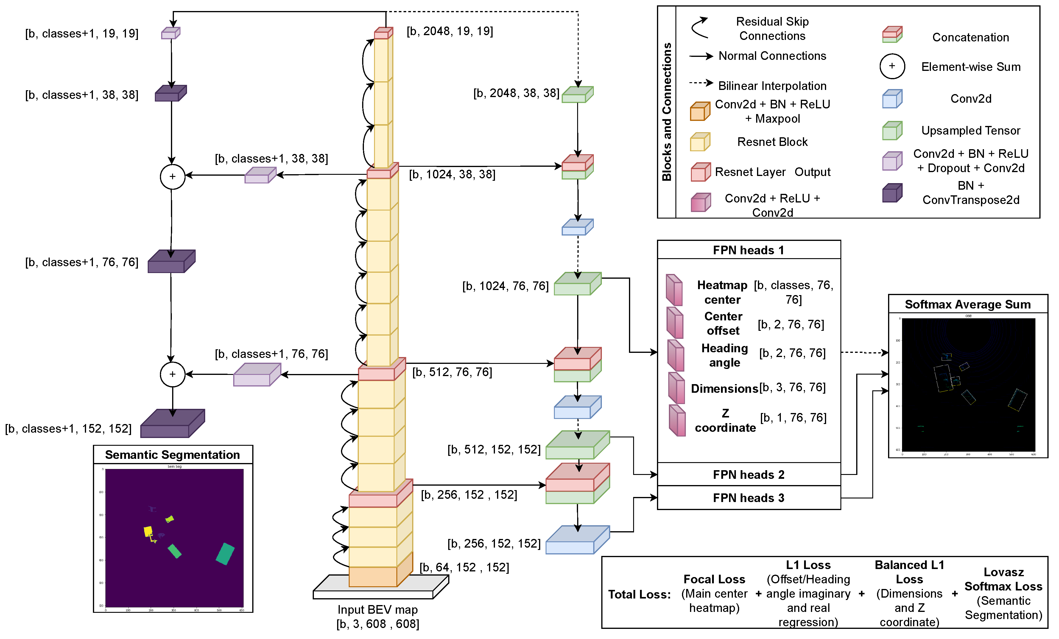
13], we extended it to also perform semantic segmentation using our synthetic dataset and a bigger version of the encoder, ResNet-50. The resulting design of our multi-task CNN is presented on
Figure 1, with a total of 45.212.563 parameters. One important observation is that neither the simulator nor the r2b dataset report the intensity values of each LiDAR point, so this channel did not affect the performance of the network. In a real life application, where LiDARs do report these values, they can be valuable for the network to distinguish one object from another or foreground from background. For this reason the intensity channel is maintained in our final design.
In the architecture design, shown in
Figure 1, we chose the ResNet-50 backbone and KeyPoint Feature Pyramid Network (FPN) for 3D object detection, and Fully Convolutional Network (FCN) for semantic segmentation.
ResNet-50 [
33] offers a good balance between depth and computational cost, making it suitable for real-time applications. Its skip connections alleviate the vanishing gradient problem, enabling effective training of deep networks. While newer architectures exist, ResNet-50 remains widely adopted, with extensive pre-trained models and strong empirical evidence of its effectiveness across various tasks.
KeyPoint FPN [
34] complements the ResNet-50 backbone by enhancing feature representation and spatial awareness across different scales. It efficiently extracts hierarchical features and aggregates contextual information, which is crucial for accurately localizing objects and keypoints in 3D space. While more recent FPN variants exist, KeyPoint FPN strikes a balance between performance and computational efficiency.
FCN [
35] is a seminal architecture for semantic segmentation, providing an end-to-end solution for pixel-wise classification tasks. Despite newer approaches achieving slightly higher accuracy, FCN remains widely used due to its simplicity, interpretability, and ease of implementation. Its fully convolutional nature enables efficient inference and end-to-end training, making it suitable for various real-world applications.
By leveraging these architectures, we aim to strike a balance between performance, efficiency, and ease of implementation, ensuring robust and practical solutions for 3D object detection and semantic segmentation tasks. While they may not represent the cutting-edge, their proven track record and suitability for deployment in resource-constrained environments make them pragmatic choices for this design.
Centralized Map Builder: For the centralized data aggregation and map building some premises are considered. Since we are integrating multiple detections from multiple sources over time in a closed indoor environment, an object can not simply vanish from the detected area from one iteration to the other, nor can two or more object occupy the same area at the same time, confidence and number of detections with the same class are used to distinguish false positive, false negative and double detections in a determined area. The algorithm does not consider the case where a person sits on a chair for example, in this case the CNN could be trained with another class named "sitting person". Also, the situation where a robot moves under a table is not covered by this algorithm, in this case the semantic segmentation part of the CNN could be trained to predict the table’s legs instead of predicting the full table segmentation. Furthermore, a basic requirement of a tracking and re-identification system is to assign a single id number for each instance in the map. If an instance leaves the field of view of every source’s sensor, when it reappears it should be assigned to the same id number as before.
Another consideration is that the detection robots have a self global localization algorithm running, and they publish their poses together with the detections from the CNN. This way, local detection poses can be transformed in global poses and detection robots can also be integrated in the id table.
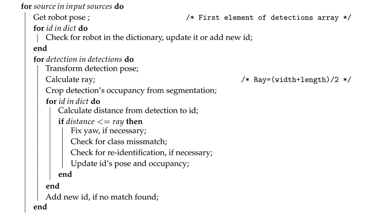
In summary, the centralized algorithm runs at 10hz and at each iteration it synchronizes the received detections and segmentation from all sources and maintain a dictionary table where each line represents an instance with an id number and the columns contain a characteristic of the particular instance, such as class, 2D pose, ray, and occupancy mask. First it iterates over each source, then it iterates over the dictionary for a match with the detection robot (source) and transforms every detection from that robot to global poses. For each transformed detection in iterates over the dictionary for a match and, when necessary, deals with miss class, twists yaw angle, updates the dictionary and add a new instance when no match is found. After every source iteration, it checks for doubled detections in the dictionary and builds the final map on top of the empty environment map. The long-term time complexity of the centralized algorithm is
. Where
r is the number of detection sources,
m the size of the id dictionary and
d the number of detections. The pseudo algorithm of the python script is given in Algorithm A1 on
Appendix A.
Three modes are available for the final map. On Instance Segmentation Mode, each instance colored with a unique color. On Semantic Segmentation mode, each class is colored with a unique color. On Gray-scale Occupancy Mode, each pixel is either unknown, occupied or unoccupied. This third mode is published in a map topic using OccupancyGrid ROS2 message type, for navigation and/or sensor filtering.
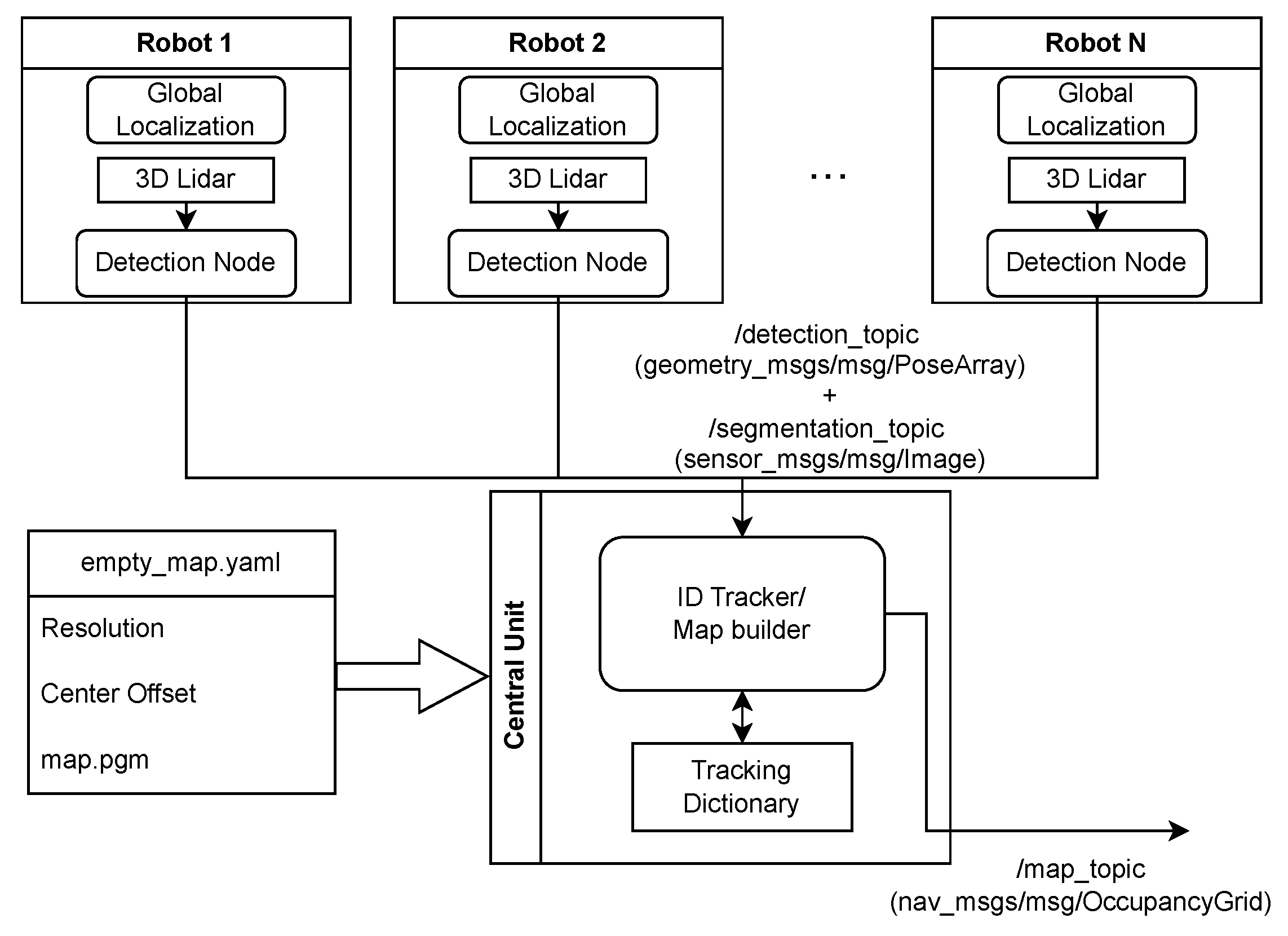
A diagram of the full system is presented in
Figure 2. Initially, the "z" position and height elements of each detection where meant to be used to help the distinction among detected objects, so a custom ROS2 msg type was created to contain these information. However, in order to test the system in one single computer, we had to run the same simulation scenario multiple times, one for each detection source, then save the detections and segmentation images into rosbags, merge them together and run the merged rosbag with the centralized node. The issue is that rosbags does not support custom message types, so we adapted the original algorithm to use the legacy
PoseArray ROS2 message type. With this workaround solution, each pose in the array have 7 fields of
float64 type, used for storing positions "x", "y", class, confidence, width, height and yaw angle. Thus disregarding the "z" position and height information of each detection.
Evaluation metrics: In assessing the performance of various tasks within my system, distinct evaluation metrics were employed to effectively gauge their efficacy. For semantic segmentation and occupancy mapping, the evaluation relied on per-pixel precision, recall, and Intersection over Union (IoU), averaged across all available samples.
Conversely, for object detection, Average Precision (AP) served as the primary metric for each class and Mean Average Precision (mAP) for classes-wide evaluation. Derived from the area under the precision-recall curve, with an IoU threshold typically set at 0.5 to determine true positives, false positives and false negatives. The area is calculated in this paper using trapezoidal area function interpolating all points for calculation. This metric aligns with established standards such as those observed in the Pascal VOC 2007 and DOTA datasets [
36].
The absolute errors in positions "x", "y" and angle "yaw" are calculated to every instance in the final id dictionary, then averaged to give an estimation about the performance of final system localization of the movable objects.
By utilizing these evaluation metrics, a thorough assessment of system performance was achieved across diverse tasks, ensuring a comprehensive understanding of its capabilities and limitations.
4. Results
The neural network training occurred for more than 300 epochs with cosine learning rate decay [
37], starting with a learning rate of 0,001. Different batch sizes were used, more specifically a batch size 4 for an onboard
NVIDIA RTX3070 and 10 for a
V100. For data augmentation, each sampĺe had a probability of horizontal flip, random translation on LiDAR’s "x" axis and random rotation on LiDAR’s "z" axis. As the automated dataset generation tool is available, the dataset was also increased during training with more samples of classes with low evaluation scores. The weights obtained in the epoch with the lowest total loss on valuation set were selected for the following experiments.
Primary, these weights were used to make predictions on test set in order to evaluate the CNN model. The metrics described in
Section 3 were used to evaluate the semantic segmentation and oriented bounding boxes detection. Semantic segmentation and oriented object detection results are presented in
Table 1. Mean Average Precision calculation varying the IoU threshold from 10% to 90% with 10% pace resulted in
, and from 50% to 95% with 5% pace resulted in
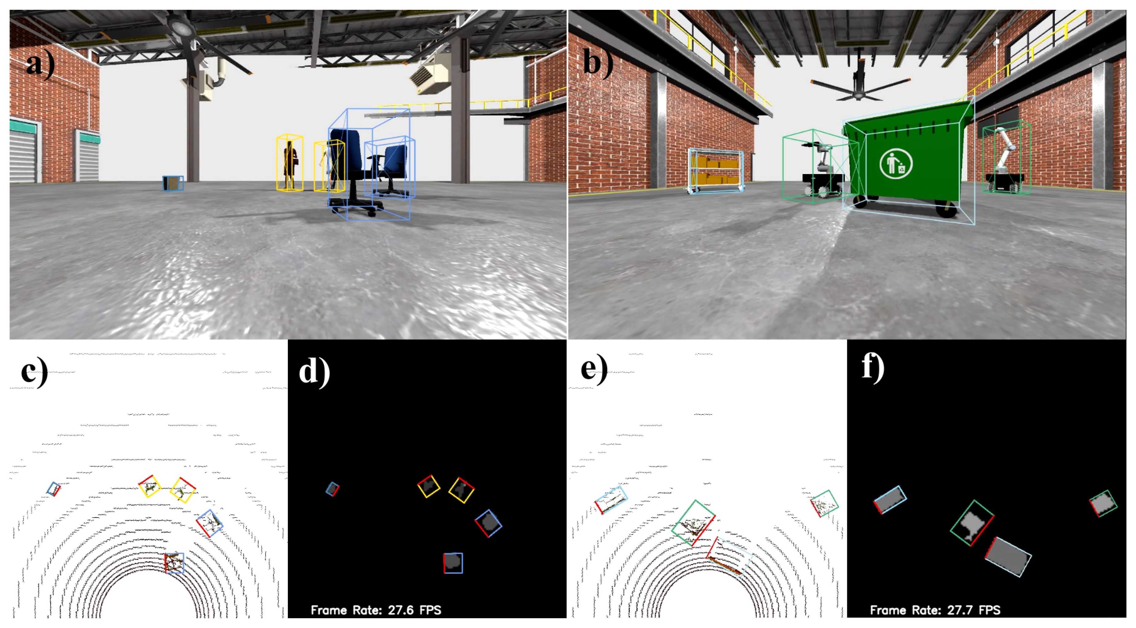
. For qualitative results, Video S1 in Supplementary Materials was created using each sample of the test set, with the BEV map input, oriented bounding box visualization, segmentation prediction and RGB image with 3D bounding box visualization. Two frames of the Video S1 are shown on
Figure 3.
The r2b dataset consists of sequences of collected sensor data stored in rosbags [
38]. The sequences have data from a 3D LiDAR similar to the one we simulated, and two of these sequences contain humans walking in front of a mobile robot:
r2b_storage and
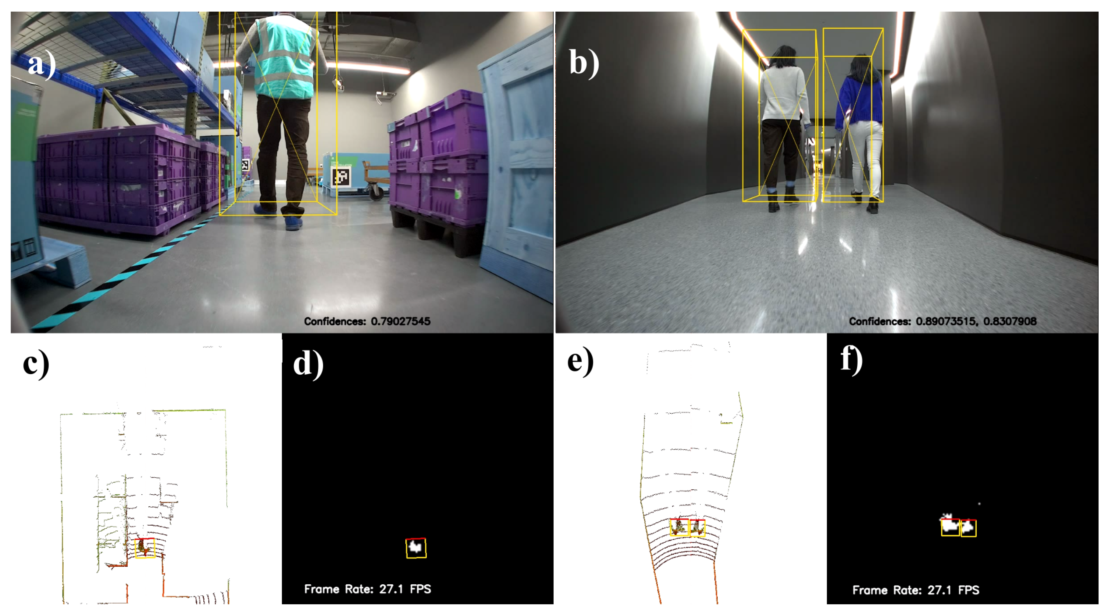
r2b_hallway. Due to the unavailability of a real-world dataset for object detection and segmentation on LiDAR BEV maps with the same simulated movable objects, each frame of the two sequences were annotated and used to evaluate our model on the person class. Results are given in
Table 2, with semantic segmentation and oriented bounding boxes evaluation. Varying the IoU threshold from 10% to 90% with 10% pace, oriented object detection resulted in
, and with the variation from 50% to 95% with 5% pace resulted in
. Video S2 with the predictions on each frame was also made for the sequences and two frames of the Video S2 are presented in
Figure 4 for qualitative analyses.
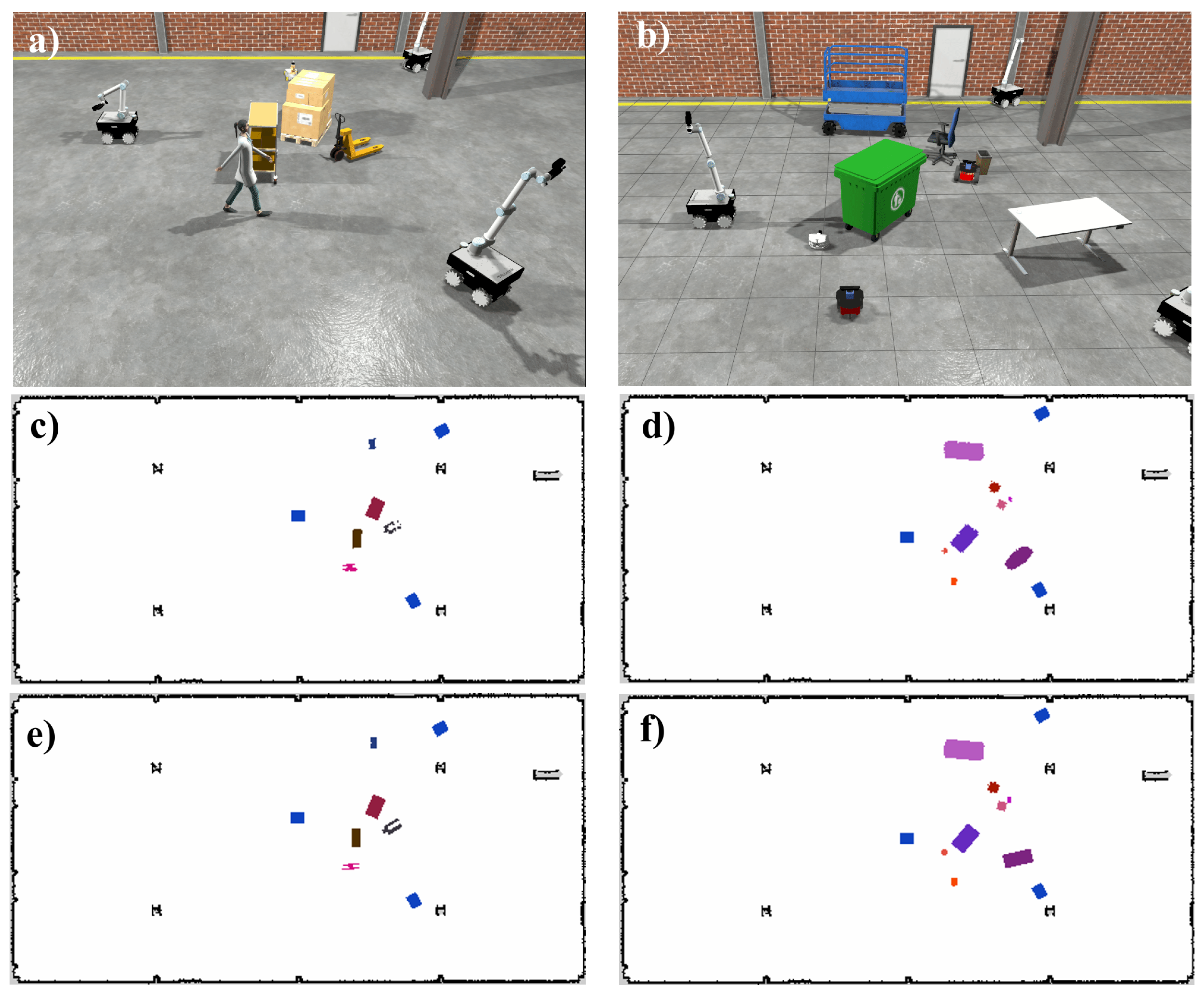
To evaluate the performance of the data aggregation on the centralized node, two simulated scenarios were created using three instances of the RB-Kairos robot mounted with the LiDAR sensor and one instance of each class to be mapped and tracked. Final map segmentation evaluation and final 2D localization error are presented in
Table 3.
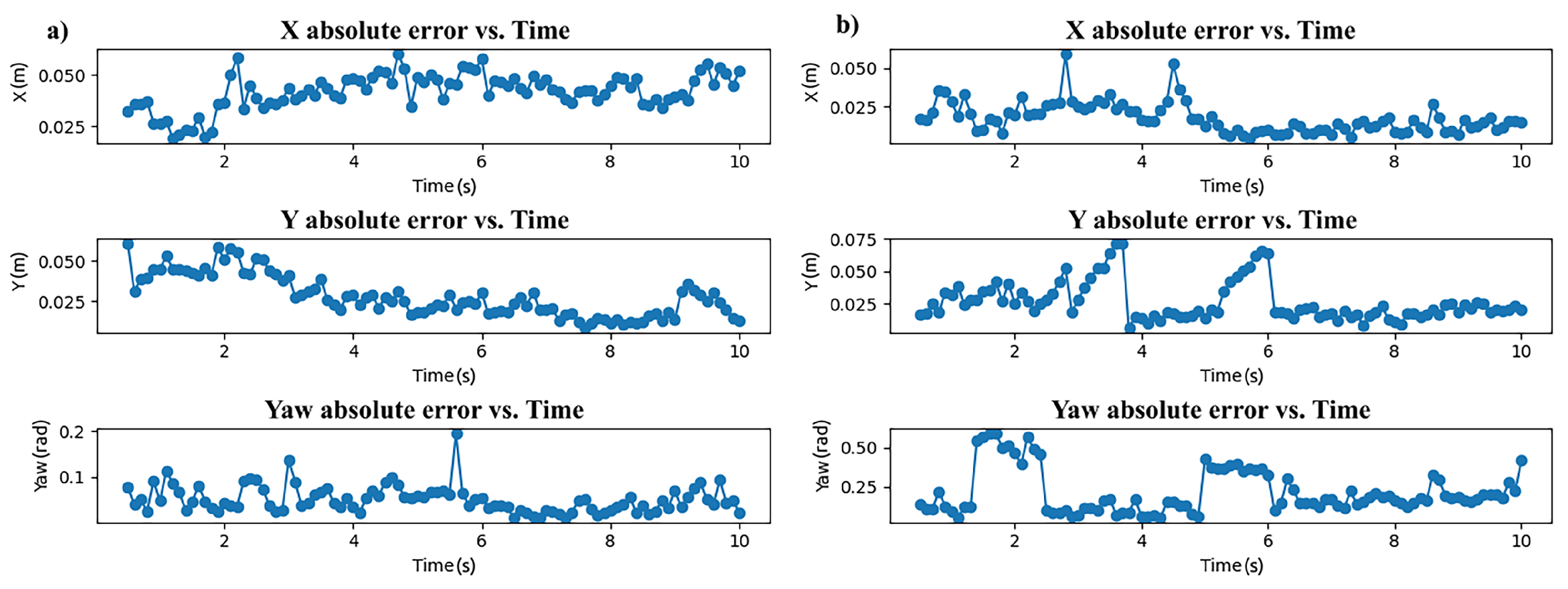
Figure 5 contains graphs of absolute localization errors for both scenarios in time. Since each detection robot also reports its localization with good precision, their class was not considered in evaluation. A frame of each simulation scenario with their respective semantic occupancy map and ground truth map are shown in
Figure 6. Video S3 contains an animation of both scenarios with their respective semantic occupancy map and ground truth map.
Table 4 contains the average timing for each step of our proposed pipeline, considering our specific hardware.
5. Discussion
The overall scores of precision, recall and IoU metrics shown in
Table 1 indicates that the model can predict the class label of each pixel without many false positives nor false negatives, the IoU indicates that it predicts more than 45% of all classes’ pixels, fairly indicating if each pixel is occupied or not by one determined class. The person class is the one with lower IoU score among the classes, probably due to the predictions of arms and legs during walking animations and frequent occlusions in the test set.
The mean average precision on
Table 1 represent that the model can predict the oriented bounding boxes in the 2D BEV domain well. Even though it is evaluated in another dataset thus not possible to directly compare with our network, the state-of-the-art in
DOTA 1.5 is
RTMDet-R [
16] with
. On the qualitative results of the test set, its notable that on specific classes, the yaw angle prediction of the instances performs poorly and the reason is that these classes have too symmetric models, making it hard to determine their direction since just one side of the objects is represented in the LiDAR data.
The quantitative results on real-world data, shown in
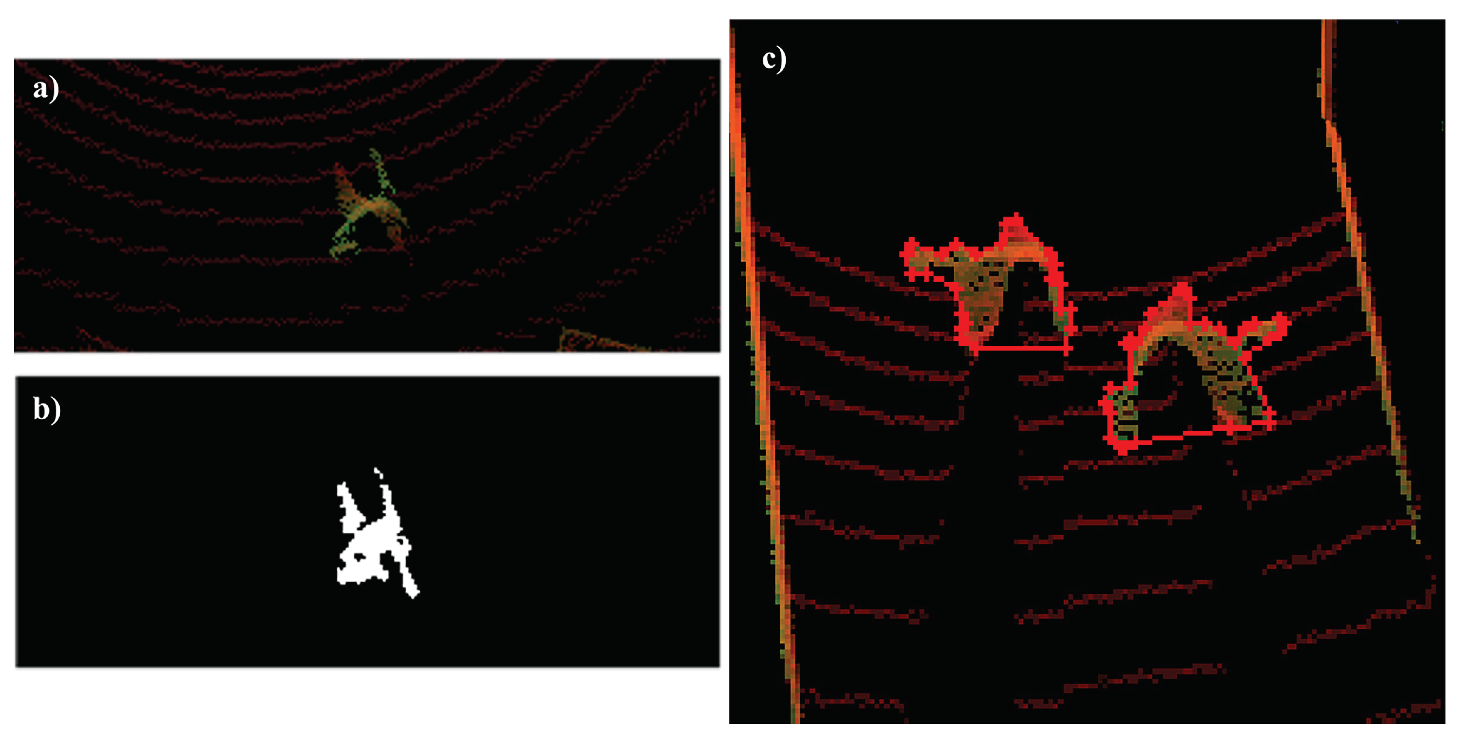
Table 2, indicates that even with only synthetic training data the model can partially predict and segment the person class in the real-world scenarios. One reason for the decrease on each metric score is the difference between simulation and real scenario domains, where the walking action is more natural than in the simulated animation. Also, in the first sequence the person is carrying a box and in the training set we only used generic walking animations. Other reason is the high difficulty level on manually annotating the ground truth, since only the robots’ perspective of one side of the humans is available, it is hard to determine and annotate both the direction and the segmentation of them in the 2D BEV space. These reasons can be visualized on
Figure 7, and they reinforce the difficulty of creating a real-world data set for this multi-task neural network, at least two sensors on opposite sides of the target object would be needed to annotate the segmentation task and a gyroscope to determine the direction of objects that do not have internal sensors.
For the centralized node, both the quantitative and qualitative results indicate a fast and accurate data aggregation on the tasks of tracking the objects locations and mapping their occupancy. The yaw predictions are post-processed for dealing with symmetric classes and random 180 degrees flips from frame-to-frame. On the second scenario, one of the models leaves the field of view of all three detection robots, and comes back after a few seconds being re-identified with same ID as before in the dictionary.
Considering the LiDAR sensor’s frequency of 10hz, it is desired to process the hole system pipeline in between LiDAR data acquisitions. As shown in
Table 4, the only step that makes this processing impossible is the first one. This step is only necessary because we need to transform the ROS message type coming from the simulation bridge into an array containing each point’s location. On real applications, the sensor data is available locally to the robots through it’s driver, and the ROS message conversion could be bypassed by a simple wrapper directly on the driver’s readings.
Figure 1.
Architecture of Keypoint Feature Pyramid Network and Fully Convolutional Network with ResNet-50 encoder backbone. To ease visualization, Segmentation is colored and 3D detection represented with 2D oriented bounding boxes. Source: Authors.
Figure 1.
Architecture of Keypoint Feature Pyramid Network and Fully Convolutional Network with ResNet-50 encoder backbone. To ease visualization, Segmentation is colored and 3D detection represented with 2D oriented bounding boxes. Source: Authors.
Figure 2.
Design of system nodes for data aggregation and map building. Source: Authors.
Figure 2.
Design of system nodes for data aggregation and map building. Source: Authors.
Figure 3.
First and second frames predictions. RGB image with 3D bounding boxes visualization (a and b, respectively), BEV input with oriented bounding boxes (c and e, respectively), and semantic segmentation with oriented bounding boxes (d and f, respectively). Source: Authors.
Figure 3.
First and second frames predictions. RGB image with 3D bounding boxes visualization (a and b, respectively), BEV input with oriented bounding boxes (c and e, respectively), and semantic segmentation with oriented bounding boxes (d and f, respectively). Source: Authors.
Figure 4.
First and second frames predictions on r2b dataset. RGB image with 3D bounding boxes visualization (a and b, respectively), BEV input with oriented bounding boxes (c and e, respectively), and semantic segmentation with oriented bounding boxes (d and f, respectively). Source: Authors.
Figure 4.
First and second frames predictions on r2b dataset. RGB image with 3D bounding boxes visualization (a and b, respectively), BEV input with oriented bounding boxes (c and e, respectively), and semantic segmentation with oriented bounding boxes (d and f, respectively). Source: Authors.
Figure 5.
Absolute localization errors for first and second simulated scenarios (a and b, respectively). Source: Authors.
Figure 5.
Absolute localization errors for first and second simulated scenarios (a and b, respectively). Source: Authors.
Figure 6.
First and second simulated scenarios (a and b, respectively). Semantic occupancy map generated by the central node for scene one (c) and two (d). Semantic occupancy map ground truth for scene one (e) and two (f). Source: Authors.
Figure 6.
First and second simulated scenarios (a and b, respectively). Semantic occupancy map generated by the central node for scene one (c) and two (d). Semantic occupancy map ground truth for scene one (e) and two (f). Source: Authors.
Figure 7.
Synthetic dataset BEV sample and its automatically generated segmentation ground truth (a and b, respectively). BEV sample of r2b dataset (c), segmentation obtained with the polygon (contour in red) though manually clicked vertices, blind sides were annotated in a non-convex manner. Source: Authors.
Table 1.
Test Set Semantic Segmentation Evaluation: Per-pixel average values for Precision, Recall, and IoU. Average Precisions and mAP for Oriented Bounding Boxes Evaluation.
Table 1.
Test Set Semantic Segmentation Evaluation: Per-pixel average values for Precision, Recall, and IoU. Average Precisions and mAP for Oriented Bounding Boxes Evaluation.
| |
Precision (%) |
Recall (%) |
IoU (%) |
(%) |
| 0: Background |
99.72 |
99.83 |
99.55 |
- |
| 1: Person |
61.12 |
71.21 |
47.54 |
85.20 |
| 2: Trash Bin |
81.35 |
86.60 |
72.60 |
98.71 |
| 3: Chair |
87.20 |
89.25 |
79.39 |
99.96 |
| 4: Pallet Box |
69.85 |
62.62 |
48.82 |
88.48 |
| 5: Table |
92.82 |
90.21 |
84.35 |
100.00 |
| 6: Trash Can |
96.77 |
89.37 |
88.54 |
99.74 |
| 7: Cart |
73.15 |
87.99 |
64.96 |
94.51 |
| 8: Pallet Jack |
70.54 |
69.88 |
51.29 |
100.00 |
| 9: Youbot |
74.75 |
77.91 |
60.24 |
92.12 |
| 10: RB-Kairos |
44.39 |
87.60 |
39.77 |
98.11 |
| 11: Pioneer 3-DX |
79.43 |
87.11 |
70.42 |
96.07 |
| 12: Robotino |
83.88 |
76.34 |
65.83 |
94.84 |
| 13: Pioneer 3-AT |
85.88 |
80.45 |
71.37 |
93.01 |
| 14: Lift |
94.54 |
91.88 |
87.20 |
85.05 |
| Total w/o background |
80.24 |
82.06 |
68.79 |
mAP = 94.70 |
Table 2.
Subset of r2b_dataset Semantic Segmentation Evaluation: Per-pixel average values for Precision, Recall, and IoU. Mean Average Precision for Oriented Bounding Boxes Evaluation.
Table 2.
Subset of r2b_dataset Semantic Segmentation Evaluation: Per-pixel average values for Precision, Recall, and IoU. Mean Average Precision for Oriented Bounding Boxes Evaluation.
| |
Precision (%) |
Recall (%) |
IoU (%) |
(%) |
| 0: Background |
99.96 |
96.80 |
96.76 |
- |
| 1: Person |
58.77 |
58.78 |
37.69 |
40.54 |
Table 3.
Merged Map Semantic Evaluation: Per-pixel Precision, Recall, and IoU; Localization Evaluation: X, Y, Yaw errors (*total values calculated considering symmetric classes).
Table 3.
Merged Map Semantic Evaluation: Per-pixel Precision, Recall, and IoU; Localization Evaluation: X, Y, Yaw errors (*total values calculated considering symmetric classes).
| |
Precision (%) |
Recall (%) |
IoU (%) |
X error (m) |
Y error (m) |
Yaw error (rad) |
| 0: Person |
63.92 |
67.86 |
49.19 |
0.0695 |
0.0152 |
0.08 |
| 1: Trash Bin |
71.84 |
79.31 |
62.63 |
0.0082 |
0.0139 |
2.90 |
| 2: Chair |
85.84 |
78.14 |
69.52 |
0.0149 |
0.0072 |
0.08 |
| 3: Pallet Box |
95.05 |
88.21 |
84.38 |
0.0089 |
0.0134 |
0.02 |
| 4: Table |
87.20 |
84.17 |
74.82 |
0.0246 |
0.0316 |
0.56 |
| 5: Trash Can |
94.38 |
91.88 |
87.32 |
0.0169 |
0.0135 |
1.55 |
| 6: Cart |
91.97 |
92.22 |
85.51 |
0.0101 |
0.0254 |
0.04 |
| 7: Pallet Jack |
81.56 |
54.17 |
48.32 |
0.0707 |
0.0332 |
0.07 |
| 8: Youbot |
68.45 |
60.52 |
48.17 |
0.0500 |
0.0537 |
0.05 |
| 9: RB-Kairos * |
- |
- |
- |
- |
- |
- |
| 10: Pioneer 3-DX |
89.97 |
76.68 |
71.48 |
0.0214 |
0.0894 |
0.49 |
| 11: Robotino |
85.77 |
78.27 |
70.72 |
0.0188 |
0.0146 |
0.18 |
| 12: Pioneer 3-AT |
87.95 |
79.38 |
71.96 |
0.0122 |
0.0211 |
0.09 |
| 13: Lift |
91.06 |
75.41 |
70.55 |
0.0237 |
0.0333 |
0.38 |
| Total |
84.55 |
78.71 |
70.22 |
0.0298 |
0.0274 |
0.135 |
Table 4.
Average timing values in seconds for each part of the pipeline.
Table 4.
Average timing values in seconds for each part of the pipeline.
| Pointcloud2_msg to Array |
Points Filtering |
BEV Building |
Prediction |
Data Aggregation |
| 0.1485 |
0.0009 |
0.0090 |
0.0406 |
0.0015 |

