
Submitted:
09 October 2024
Posted:
10 October 2024
You are already at the latest version
Abstract
The monitoring of fog density is of great importance in meteorology and its applications in environment, aviation and transportation. Nowadays, vision-based fog estimation from images taken with surveillance cameras has made a great supplementary contribution to the scarcely traditional meteorological fog observation. In this paper, we propose a new Random Forest (RF) approach for image-based fog estimation. In order to reduce the impact of data imbalance on recognition, the StyleGAN2-ADA (generative adversarial network with adaptive discriminator augmentation) algorithm is used to generate virtual images to expand the data of low proportions. Key image features related to fog are extracted, and an RF method, integrated with the hierarchical and k-medoids clustering, is deployed to estimate the fog density. The experiment conducted in Sichuan in February 2024 shows that the improved RF model has achieved an average accuracy of fog density observation to 93%, 6.4% higher than the RF model without data expansion, 3%-6% higher than the VGG16, the VGG19, the ResNet50, and the DenseNet169 with or without data expansion. What is more, the improved RF method exhibits a very good convergence as a cost-effective solution.
Keywords:
Fog density
; data augmentation
; random forest
; generative adversarial network
; hierarchical clustering
; fog-relevant features
1. Introduction
Fog, a weather phenomenon of visual obstruction, is formed by tiny water droplets or ice crystals floating in the air [1]. The observation of fog plays a significant role in weather and climate analysis inn meteorology. In daily life, fog forecasting have important applications for aviation safety, agricultural production, and environmental monitoring [1,2]. According to its density, fog is typically classified into five grades as the light fog, the moderate fog, the dense fog, the thick fog, and the very thick fog. The horizontal visibility caused by different fog density is shown in Table 1 [3].
In early fog meteorological observation, observers identified targets at varying distances from their location to estimate fog density using the naked eye [4]. Currently, automated instruments such as transmissometers and scatterometers [4,5] are employed to observe horizontal visibility, which is derived from atmospheric optical processes. However, automatic observation systems often suffer from limited representativeness when local optical characteristics differ from those of the broader environment. Additionally, large-scale and high-density deployments of these systems are prohibitively expensive. Satellite-based fog remote sensing also faces challenges, particularly due to cloud interference, which reduces accuracy [6]. In recent years, the widespread use of surveillance cameras across various industries has sparked research into optical recognition, image denoising, and fog visibility observation, becoming a focal point in the fields of image recognition and artificial intelligence [7,8,9,10,11,12,13,14,15,16].
Currently, fog density estimation based on optical images can be divided into two categories: traditional computer vision methods and neural network-based approaches.
Traditional computer vision methods estimate visibility using image processing techniques, extracting features such as Region of Interest (ROI) extraction, edge detection, vanishing points, and horizon detection, and applying linear statistical equations to estimate fog visibility. Among these methods, Busch et al. [17] introduced a visibility estimation method using B-spline wavelet transforms. Hautière et al. [18] calculated fog visibility distance by extracting road and sky regions. Negru et al. [19] proposed a method for detecting fog from moving vehicles by analyzing inflection points and the horizon in images. Guo et al. [20] developed a visibility estimation technique using ROI extraction and camera parameter estimation. Wauben et al. [21] presented a series of techniques for fog visibility estimation, including edge detection, contrast reduction between consecutive images, decision tree methods, and linear regression models. Yang et al. [22] introduced an algorithm for visibility estimation under dark, snowy, and foggy conditions, combining dark channel prior, support vector machines, and weighted image entropy. Cheng et al. [23] proposed an improved visibility estimation algorithm using piecewise stationary time series analysis and image entropy, incorporating subjective assessments to judge fog and haze visibility. Zhu et al. [24] estimated fog density in weather images by analyzing saturation and brightness in the HSV color space. Despite the effectiveness of these image feature-based methods, they face challenges such as limited generalization ability and low flexibility.
Deep learning has achieved remarkable success in computer vision (CV), natural language processing, and video/speech recognition [25]. Numerous studies have applied these methods to fog image estimation. Tang et al. [7] predicted visibility in various weather conditions by training a random forest model [8] using dark channel, local contrast, and saturation features. Jonnalagadda and Hashemi [11] introduced an autoregressive recurrent neural network that leverages the temporal dynamics of atmospheric conditions to predict visibility. Li et al. [9] enhanced visibility detection accuracy through transfer learning, where pre-trained models improve prediction accuracy without requiring large amounts of training data. Li et al. [12] proposed a meteorological visibility estimation method based on feature fusion and transfer learning, integrating multiple data sources for more accurate estimations. Lo et al. [13] experimentally evaluated a transfer learning method using particle swarm optimization (PSO) for meteorological visibility estimation. Liu et al. [14] introduced an end-to-end visibility estimation network (FGS-Net) based on statistical feature streams, which demonstrated high effectiveness in fog-prone areas. Choi et al. [15] developed an automatic sea fog detection and visibility estimation method using CCTV images, achieving accurate sea fog detection and visibility distance estimation. Zhang et al. [16] proposed a deep learning method for visibility estimation in traffic images, where deep quantification techniques improved visibility prediction accuracy.However, these methods typically rely on training with large, balanced datasets. While deep learning models such as VGG16 and ResNet50 perform well on large-scale datasets, their accuracy significantly declines when sufficient data is not available. In this study, we compare the performance of VGG16, ResNet50, DenseNet169, and our improved Random Forest (RF) model. VGG16/19 [26] employ multiple convolutional layers and max-pooling for feature extraction, though their depth results in high computational costs. ResNet50 [27] addresses the vanishing gradient problem using residual modules, enabling deeper networks with better performance on complex tasks. DenseNet169 [28] improves efficiency through dense connections, while Random Forest [29] enhances model stability by reducing overfitting in decision trees.Furthermore, the dataset we collected often lacks extreme data, resulting in a low proportion of extreme categories. This uneven distribution creates an imbalanced dataset for training purposes, presenting additional challenges in model performance.
When the dataset is unevenly distributed, as observed with the QVEData used in [16] and the private dataset in [30], the methods suffer from poor generalization ability. The scarcity of image samples under conditions of dense fog and very dense fog limits the diversity available during training, leading to reduced estimation accuracy. Moreover, algorithm convergence remains a significant challenge. Many traditional methods require extended training times to achieve convergence, especially when handling complex foggy images [31,32]. In cases of imbalanced or insufficient data, overfitting becomes a common issue, resulting in poor algorithm convergence and reduced method efficiency.
To improve the performance of the RF model in estimating fog on insufficient and imbalanced data, we propose a GAN-based data augmentation technique to increase the proportion of low-representation grades in the dataset. This approach reduces reliance on naturally imbalanced datasets, where high fog density grades are underrepresented. By applying StyleGAN2-ADA [33] for dataset augmentation, the issue of imbalanced data distribution is mitigated. The generated virtual images increase and balance the dataset across different fog density grades, addressing training challenges posed by limited and imperfect data. Furthermore, by incorporating hierarchical and k-medoids clustering within the Random Forest model [8], this method enhances observation accuracy and accelerates training convergence on imbalanced datasets, outperforming algorithms such as VGG16, VGG19, ResNet50, and DenseNet169.
2. Data and Methodology
2.1. Experiment and Data
The dataset used in this study was collected from an experiment conducted on the National Highway G318 near the Erlang Mountain Tunnel in Tianquan County, Sichuan Province, China, in July 2023. A traffic meteorological station was set up, equipped with sensors for temperature, pressure, humidity, wind, and precipitation observation, along with a high-definition camera and a visibility meter. The GM-VTF306B visibility meter, capable of measuring visibility from 10 to 10,000 meters, was used in the experiment. The dataset includes 1,203 highway images along with their corresponding visibility observations. The images were classified into five grades: light fog, moderate fog, dense fog, thick fog, and very thick fog, based on their visibility measurements [3]. For normalization, the original images were resampled to 512x512 pixels, as illustrated in Figure 1.
2.2. Data Augmentation
The GAN architecture, first proposed in [34], is a framework for generative models through adversarial training, as illustrated in Figure 2. It consists of a pair of models known as the generator (G) and the discriminator (D). Both networks are fully connected neural networks. The generator creates fake images (which do not exist in the original training set) using noise input, while the discriminator tries to distinguish these fake images from real images in the original training set. The entire framework resembles a two-player minimax game, where the generator aims to minimize its objective function, and the discriminator seeks to maximize its objective function. Consequently, G learns to generate images that D evaluates as real, while D learns to accurately distinguish between fake and real images. By alternating these processes, G generates images that closely resemble real ones.
2.3. Extraction of Image Features Related to Fog Density
In foggy weather, images typically display low contrast, muted colors, and saturation shifts due to the scattering and absorption of atmospheric particles. To investigate simple yet effective fog-related features, we test sixteen Natural Scene Statistics (NSS) features. These include the variance of Mean Subtracted Contrast Normalized (MSCN) coefficients, dark channel, colorfulness, sharpness, sharpness variance coefficient, image entropy, saturation-value, chroma, chroma variance, Weber contrast of luminance, local contrast, contrast energy (gray), contrast energy (yb), contrast energy (rg), gradient magnitude, and color variance. These features are analyzed to assess images with varying fog density. Our goal is to explore several effective fog-relevant features.
(1) Coefficient of MSCN Variance [35]:
where, , are spatial indices, M and N are image dimensions, is a 2D circularly symmetric Gaussian weighting function sampled out to 3 standard deviations () and rescaled to unit volume, and is the gray version of a natural image I.
(2) Dark Channel [36]:
where, denotes a color channel of image I, represents a local patch centered at x, and y is the pixel around x in .
(3) Colorfulness [37]:
where, , , , and represent the mean and variance values for and channels of image I in the local patch centered at x, and they are defined as
(4) Sharpness [35]:
with
where, represents the grayscale version of the target imageI, and denotes a 2D Gaussian weighting function with circular symmetry.
(5) Coefficient of Sharpness Variance [35]: The coefficient is defined for a local patch , centered at point x in image I, as
with
where is the size of .
(7) Saturation-Value [39]:
(8) Chroma [37]: Let be the pixel values of an image I in the CIELab space, and the chroma is defined as
(9) Variance of Chroma [37]: This variance is defined within a local patch , centered at point x in imageI, as
(10) Weber Contrast of Luminance [40]:
where represents the background luminance, and denotes the contrast in luminance for a pixel x within an image patch . The background luminance is derived by applying a low-pass filter to the luminance component v of HSV color space.
(11) Local Contrast [40]:
(12) Contrast Energy [38]:
Contrast Energy (gray):
where is the intensity (gray value) of the pixel, is the mean intensity of the region and N is the total number of pixels in the region.
Contrast energy (yb):
where is the yellow-blue value for the pixel and is the mean value of the yellow-blue component in the region.
Contrast energy (rg):
where is the red-green value for the pixel and is the mean value of the red-green component in the region.
(13) Gradient Magnitude [42]:
where is the gradient in the horizontal direction and is the gradient in the vertical direction at pixel .
(14) Color Variance [42]:
where is the mean color value, and represents the variance of the color distribution.
2.4. Deep Learning Approaches: VGG16, VGG19, ResNet50, DenseNet169 and the Improved Random Forest
VGG16 and VGG19 [26] are the two representative algorithms of the VGGNet, containing 13 and 16 convolutional layers, respectively. They extract features from input images using multiple 3×3 convolutional filters with a stride of 1px. To accelerate the convergence of the model, the VGG series uses ReLU activation function and applies max-pooling in the pooling layers to downsample the features. However, due to the deep network depth of the VGG models, the number of parameters is relatively large, which may lead to higher computational costs when handling complex image tasks.
ResNet50 [27] effectively addresses the vanishing gradient problem in deep networks by introducing residual modules, making it possible to train deeper networks. ResNet50 includes 48 convolutional layers, 1 max-pooling layer, and 1 fully connected layer. Compared to the VGG series, the ResNet architecture is more complex, but it performs better in feature extraction and classification tasks, particularly in handling complex textures and detailed features in images.
DenseNet169 [28] ensures efficient reuse of features at different levels by employing densely connected layers. DenseNet169 consists of 169 layers. Due to its densely connected nature, it significantly reduces the number of parameters and improves the training efficiency of the model. DenseNet has demonstrated strong classification capabilities and generalization abilities when processing high-resolution and diverse image data.
Traditional Random Forest models make predictions by constructing multiple random decision trees, with each tree randomly selecting a subset of features from the input for training [29]. Through ensemble learning, the Random Forest model reduces the risk of overfitting associated with individual decision trees, thereby enhancing the model’s stability.
When observing fog concentration, the data often includes various image features, resulting in high-dimensional and noisy data. This can negatively impact the performance of weak classifiers in traditional Random Forest models, leading to a decline in overall classification accuracy. To address the limitations of traditional Random Forest models in handling high-dimensional data and complex nonlinear relationships, a hybrid clustering-based method is introduced to optimize decision tree selection, improving the model’s overall performance. The specific steps are as follows:
- Hierarchical Clustering. Initially, each decision tree is treated as an independent cluster. The Dunn index is used to calculate the similarity between any two decision trees, and the two clusters with the smallest similarity are merged. This process is repeated until the number of remaining clusters reaches a predetermined value. Then, the decision tree with the best classification performance is selected from each cluster to form a new Random Forest model.
- K-Medoids Clustering. The cluster centers obtained from hierarchical clustering are used as the initial clusters for k-Medoids clustering. The similarity between the unclassified decision trees and each cluster center is calculated, and the decision trees are reassigned based on the nearest neighbor principle. Then, the decision tree with the best performance within each cluster is selected as the new cluster center. This process is repeated until the cluster centers stabilize or the maximum number of iterations is reached.
- Model Training and Prediction: The preprocessed feature data is input into the improved Random Forest model for training. The model constructs a large number of decision trees, with each tree independently predicting the fog density. The final output is the average of the predictions from all decision trees.
2.5. Assessment Method
To evaluate the effectiveness of the trained observation model in identifying fog density, the algorithm’s performance will be assessed using recognition accuracy, convergence index, data requirements, and model generalization ability. To verify the algorithm’s convergence in this experiment, a convergence index is used as an evaluation metric. The model is considered to have converged when the convergence index satisfies the following formula, indicating that the training curve stabilizes as the number of training iterations increases:
where represents the accuracy during the training process, and E is a custom-defined threshold.
3. Result
3.1. Augmented Data
Table 2 presents the initial Inception Score (IS) and Fréchet Inception Distance (FID) values for four different categories of the dataset generated by StyleGAN2-ADA. The Inception Score reflects the probability that the generated images belong to the specified category, while the FID measures the distance between the distributions of the generated images and the real images.
The composition of the new dataset is illustrated in Figure 3. In this study, images generated by StyleGAN2-ADA were utilized for model training but excluded from model testing. This approach effectively balanced the dataset by generating additional synthetic images.
3.2. Relationship between Image Features and Fog Density
To handle varying dynamic ranges across the extracted image features, a linear normalization process is applied , where denotes m’s feature, and and represent the averages of the highest 0.1% and lowest 0.1% of values for feature m, respectively. This normalization ensures that the adjusted features, , fall within the range . Figure 5(f) demonstrates the mean normalized features derived from the patches in Figure 5(a)-(e). Evidently, within the same scene depth, there are certain correlations between the visibility distance and normalized features, whether positive or negative.
Table 3 presents the Pearson Correlation Coefficient (PCC) between 16 image features and fog density. Figure 5 displays the correlation matrix of features calculated using PCC, where high absolute correlation values indicate significant redundancy between two features.
The sixteen features were fed into the Random Forest classifier to observe classification accuracy. Then, the feature with the lowest correlation was removed based on the Pearson Correlation Coefficient (PCC), and the accuracy test was repeated. This process was continued until the average accuracy reached its maximum. During the test, it was found that retaining features F1-F11 resulted in the highest classification accuracy, suggesting that these 11 features are the most important parameters for fog density estimation. Notably, sharpness (F4) was selected as a key feature despite its moderate correlation coefficient, as sharpness, which refers to the clarity of edges and details in an image, is significantly affected by light scattering in foggy weather.
3.3. Estimation of Fog Density
In this study, the dataset was divided into training, validation, and test sets in a 6:2:2 ratio. For the augmented dataset, the test set data were randomly selected from the initial dataset, while the training and validation set data were randomly selected from the augmented data.
(1) Estimation Accuracy
Table 4 presents the performance results of different models trained on the dataset without data augmentation. The experimental results indicate that the ResNet50 model achieved the highest average accuracy when data augmentation was not applied. However, the improved Random Forest model, incorporating hybrid clustering selection, performed comparably to ResNet50 in terms of average accuracy, achieving the highest accuracy under light fog, fog, and dense fog conditions.
Table 5 presents the performance of different models on the augmented dataset. With data augmentation, the estimation accuracy of all models improved significantly. Notably, the improved Random Forest model achieved further accuracy enhancements across all fog grades, reaching 89.8% in very dense fog and 91.7% in dense fog, with an average accuracy increase to 93.0%. Although the estimation accuracy of other models also improved after data augmentation, their average accuracy remained lower than that of the improved Random Forest model.
Additionally, the improved Random Forest model increased its average accuracy by 2.9% compared to the original Random Forest model, rising from 90.1% to 93.0%. This improvement is largely attributed to the effectiveness of the hybrid clustering method. By combining hierarchical clustering with k-Medoids clustering techniques, this method not only optimized the decision tree selection process but also effectively avoided the common local optimum problem encountered in traditional hierarchical clustering. Moreover, since the k-Medoids process was repeated only twice, the increase in computation time was negligible, meaning that this method significantly improved accuracy without a substantial increase in computational cost.
(2) Convergence Index
The variation of the loss function for different methods is shown in Figure 6. The improved Random Forest model meets the convergence condition after 40 training epochs, while other models, such as VGG-16 and VGG-19, require 60 to 80 epochs to reach convergence. This demonstrates that the improved Random Forest model not only outperforms other models in classification performance but also offers significant advantages in training efficiency. The model’s ability to converge quickly significantly reduces training time and computational cost.
(3) Data Requirements and Model Generalization Ability
Compared to existing deep learning methods in the literature (see Table 4), the improved Random Forest model performs exceptionally well on small datasets. Li et al. used a dataset containing 4,841 images, achieving an accuracy of 88%; Lo et al. employed a private dataset with 6,048 images, reaching a maximum accuracy of 92.72%; Liu et al. used the VID I dataset (containing 3,033 images), achieving an accuracy of 98%; Choi et al. and Zhang et al. used datasets with 5,104 and 24,031 images, respectively, with accuracies of 72% and 87%. Although Liu et al.’s method achieved higher accuracy on a larger dataset, the improved Random Forest model reached 93.0% accuracy on the small sample dataset, outperforming the methods used in [12,13,15,16] and showing only a slight difference compared to the method in [14]. This demonstrates that the improved Random Forest model has a significant advantage over other models in terms of data efficiency and estimation accuracy, even with limited data.
4. Conclusion and Discussion
In this paper we proposes an image-based fog observation method, an improved Random Forest model integrated with the hierarchical and k-medoids clustering, on the StyleGAN2-ADA data augmentation, which addressing the issue of dataset imbalance. Key fog-related features were studied. Performances of VGG16, VGG19, ResNet50, and DenseNet169 were compared and analzed. Experiment shows that the improved RF approach has gained significantly an increased observation accuracy and a decreased computational cost.
(1)The StyleGAN2-ADA for data augmentation effectively mitigated the issue of dataset imbalance. Through increasing the proportion of the dense fog grades, it reduces the risk of overfitting greatly, especially with limited dataset. Additionally, data augmentation accelerated the model’s training convergence speed by 30%-50%.
(2) Key fog-related features were identified through the feature aggregation test for fog density estimation. 5 features are discarded. 11 features which have bigger correlation with fog density were selected such as MSCN variance, dark channel, and chroma, to name a few. These features describe the fog image characteristics best, which are capable of improving both computational efficiency and estimation performance.
(3) To overcome the limitations of traditional Random Forest models in handling high-dimensional data and complex nonlinear relationships, the hierarchical and k-medoids clustering is integrated with the RF model. Performance comparison with other deep learning models , the VGG16, the VGG19, the ResNet50, and the DenseNet169, is made both on the initial dataset and the augumented dataset.
(4) When initial dataset is used, the ResNet50 model performed the best in terms of average accuracy. The improved Random Forest model matches with the ResNet50 in terms of the average accuracy, but gains high performance in lighter fog conditions.
(5) With data augmentation, the estimation accuracy of all models improved significantly. Notably, the improved Random Forest model achieved further enhancements in accuracy across all fog grades, reaching 89.8% in very dense fog and 91.7% in dense fog, with an average accuracy increase to 93.0%., which outperformed other deep learning models , with accuracy improvements ranging from 1.8% to 6.8%.
It is noted that the experiment was very short and the image dataset was limited on space and time. Despite the model’s very good performance, further validation is still needed in future work. Furthermore, the algorithm still needs optimization in practical application. A more effective feature extraction method should be developed. The classified light fog is minted with the haze, who is similar in terms of visibility but is different in local humidity. In practice, according to the meteorological regulation, the haze can be distinguished from the fog whose relative humidity is over 80%. For light fog image-based estimation, humidity observation is needed for the future work.
Author Contributions
All tasks were performed under the supervision and guidance of all involved authors. Y.C. took a lead role in data processing, article drafting, and proofreading. P.Z. focused on data collection, providing the essential datasets for our analysis. J.L. was instrumental in providing the concept. B.X took a role in project administration. All authors reviewed and commented on the original draft of the manuscript. Each author has read and agreed to the published version of the manuscript. Authorship has been limited to those who have significantly contributed to the work reported.
Funding
This research was funded by the National Natural Science Foundation of China (Grant No.41931075, 41961144015) and Observational Experiment Project of Meteorological Observation. Center of China Meteorological Administration (Grant No. GCSYJH24-21).
Institutional Review Board Statement
Not applicable.
Informed Consent Statement
Not applicable.
Data Availability Statement
The original contributions presented in the study are included in the article, further inquiries can be directed to the corresponding author.
Conflicts of Interest
The authors declare no conflicts of interest.
References
- Z. Li, “STUDIES OF FOG IN CHINA OVER THE PAST 40 YEARS,” Acta Meteorologica Sinica, vol.5, pp.616-624, 2001. [CrossRef]
- Z. Bao, Y. Tang, C. Li, et al., “Road Traffic Safety Technology Series: Highway Traffic Safety and Meteorological Impact (1st Edition),” Beijing: People’s Traffic Press, 2008, pp.1-15.
- General Administration of Quality Supervision, Inspection and Quarantine of the People’s Republic of China, and Standardization Administration of China, "Fog Forecast," Meteorological Standard, GB/T 27964-2011, Beijing: General Administration of Quality Supervision, Inspection and Quarantine of the People’s Republic of China, and Standardization Administration of China, December 30, 2011, pp. 1-6.
- Wang, Y. , Jia, L., Li, X., Lu, Y., and Hua, D., “A measurement method for slant visibility with slant path scattered radiance correction by lidar and the SBDART model," Optics Express, vol.29, no.2, pp.837–853, 2020. [CrossRef]
- Xian, J. , Han, Y., Huang, S., Sun, D., and Li, X., "Novel lidar algorithm for horizontal visibility measurement and sea fog monitoring," Optics Express, vol.26, no.2, pp.34853–34863, 2018. [CrossRef]
- Y. Li, H. Sun, and M. Xu, “The Present Situation and Problems on Detecting Fog by Remote Sensing with Meteorological Satellite,” Remote Sensing Technology and Application, vol.15, no.4, pp.223-227, 2000. [CrossRef]
- K. Tang, J. Yang, and J. Wang, “Investigating Haze-Relevant Features in a Learning Framework for Image Dehazing,” Computer Vision and Pattern Recognition, Jun. 2014. [CrossRef]
- D. Yuan, J. Huang, X. Yang and J. Cui, “Improved random forest classification approach based on hybrid clustering selection,” in 2020 Chinese Automation Congress (CAC), Shanghai, China, 2020, pp.1559-1563. [CrossRef]
- Q. Li, S. Tang, X. Peng, and Q. Ma, “A Method of Visibility Detection Based on the Transfer Learning,” Journal of Atmospheric and Oceanic Technology, vol.36, no.10, pp.1945-1956, Oct. 2019. [CrossRef]
- W. L. Lo, M. Zhu, and H. Fu, “Meteorology Visibility Estimation by Using Multi-Support Vector Regression Method,” Journal of Advances in Information Technology, pp.40-47, 2020. [CrossRef]
- J. Jonnalagadda and M. Hashemi, “Forecasting Atmospheric Visibility Using Auto Regressive Recurrent Neural Network,” in 2020 IEEE 21st International Conference on Information Reuse and Integration for Data Science, pp.209-215, Aug. 2020. [CrossRef]
- J. Li, W. L. Lo, H. Fu, and H. S. H. Chung, “A Transfer Learning Method for Meteorological Visibility Estimation Based on Feature Fusion Method,” Applied Sciences, vol.11, no.3, p.997, Jan. 2021. [CrossRef]
- Wai Lun Lo, H. Shu, and H. Fu, “Experimental Evaluation of PSO Based Transfer Learning Method for Meteorological Visibility Estimation,” Atmosphere, vol.12, no.7, pp.828-828, Jun. 2021. [CrossRef]
- Y. Li, Y. Ji, J. Fu, and X. Chang, “FGS-Net: A Visibility Estimation Method Based on Statistical Feature Stream in Fog Area,” Research Square (Research Square), Feb. 2023. [CrossRef]
- Y. Choi, H.-G. Y. Choi, H.-G. Choe, Jae Young Choi, Kyeong Tae Kim, J.-B. Kim, and N.-I. Kim, “Automatic Sea Fog Detection and Estimation of Visibility Distance on CCTV,” Journal of Coastal Research, vol.85, pp.881-885, May 2018. [CrossRef]
- F. Zhang et al., “Deep Quantified Visibility Estimation for Traffic Image,” Atmosphere, vol.14, no.1, pp.61-61, Dec. 2022. [CrossRef]
- C. Busch and E. Debes, “Wavelet transform for visibility analysis in fog situations,” IEEE Intelligent Systems, vol.13, no.6, pp.66–71, 1998.
- N. Hauti´ere, J.-P. Tarel, J. Lavenant, and D. Aubert, “Automatic fog detection and estimation of visibility distance through use of an on board camera,” Machine Vision and Applications, vol.17, no.1, pp.8–20, 2006.
- M. Negru and S. Nedevschi, “Image based fog detection and visibility estimation for driving assistance systems,” in 2013 IEEE 9th International Conference on Intelligent Computer Communication and Processing (ICCP), IEEE, 2013, pp.163–168.
- F. Guo, H. Peng, J. Tang, B. Zou, and C. Tang, “Visibility detection approach to road scene foggy images,” KSII Transactions on Internet & Information Systems, vol.10, no.9, 2016.
- W. Wauben and M. Roth, “Exploration of fog detection and visibility estimation from camera images,” in WMO Technical Conference on Meteorological and Environmental Instruments and Methods of Observation (CIMOTECO), 2016, pp.1–14.
- L. Yang, R. Muresan, A. Al-Dweik, and L. J. Hadjileontiadis, “Image based visibility estimation algorithm for intelligent transportation systems,” IEEE Access, vol.6, pp.76728–76740, 2018.
- X. Cheng, G. Liu, A. Hedman, K. Wang, and H. arXiv preprint arXiv:1804.04601, arXiv:1804.04601, 2018.
- Q. Zhu, J. Mai, and L. Shao, “A Fast Single Image Haze Removal Algorithm Using Color Attenuation Prior,” IEEE Transactions on Image Processing, vol.24, no.11, pp.3522-3533, Nov. 2015. [CrossRef]
- Junyi Chai, Hao Zeng, Anming Li, Eric W.T. Ngai, “Deep learning in computer vision: A critical review of emerging techniques and application scenarios,” Machine Learning with Applications, vol.6, 2021. [CrossRef]
- K. Simonyan and A. Zisserman, “Very deep convolutional networks for large-scale image recognition,”. arXiv:1409.1556, 2014. [CrossRef]
- He, X. Zhang, S. Ren, and J. Sun, “Deep Residual Learning for Image Recognition,” 2015. arXiv:1512.03385, 2015. [CrossRef]
- G. Huang, Z. Liu, L. van der Maaten, and K. Q. Weinberger, “Densely Connected Convolutional Networks,”. arXiv:1608.06993, 2016. [CrossRef]
- L. Breiman, “Random forest,” Machine Learnning, vol. A45, pp. 5–32, 2001.
- W. Yang, Y. Zhao, Q. Li, F. Zhu, and Y. Su, “Multi visual feature fusion based fog visibility estimation for expressway surveillance using deep learning network,” Expert Systems with Applications, vol.234, p.121151, 2023. [CrossRef]
- K. Miao, J. Zhou, P. Tao, et al., “Self-Adaptive Hybrid Convolutional Neural Network for Fog Image Visibility Recognition,” 2024.
- L. Huang, Z. Zhang, P. Xiao, et al., “Classification and application of highway visibility based on deep learning,” Trans Atmos Sci, vol.45, no.2, pp.203-211, 2022.
- T. Karras, M. Aittala, J. Hellsten, S. Laine, J. Lehtinen, and T. Aila, “Training generative adversarial networks with limited data,” in Proceedings of the 34th International Conference on Neural Information Processing Systems, pp.11, 2020.
- I. J. Goodfellow, J. Pouget-Abadie, M. Mirza, B. Xu, D. Warde-Farley, S. Ozair, A. Courville, and Y. Bengio, "Generative Adversarial Networks," in *Advances in Neural Information Processing Systems*, pp. 2672–2680, 2014. https://arxiv.org/abs/1406.2661.
- D. L. Ruderman, “The statistics of natural images,” Network: Computation in Neural Systems, vol.5, no.4, pp.517-548, Jan. 1994. [CrossRef]
- D. Makkar and M. Malhotra, “Single Image Haze Removal Using Dark Channel Prior,” International Journal Of Engineering And Computer Science, vol.33, Jan. 2016. [CrossRef]
- D. Hasler and S. E. Suesstrunk, “Measuring colorfulness in natural images,” Proc. SPIE, vol.5007, p.87, 2003.
- L. K. Choi, J. You, and A. C. Bovik, “Referenceless Prediction of Perceptual Fog Density and Perceptual Image Defogging,” IEEE Transactions on Image Processing, vol.24, no.11, pp.3888-3901, Nov. 2015. [CrossRef]
- K. Gu, G. Zhai, X. Yang, and W. Zhang, “Using Free Energy Principle For Blind Image Quality Assessment,” IEEE Transactions on Multimedia, vol.17, no.1, pp.50-63, Jan. 2015. [CrossRef]
- Berns, “Billmeyer and Saltzman’s Principles of Color Technology, 4th Edition,” John Wiley & Sons, 2021.
- A. Mittal, R. Soundararajan, and A. C. Bovik, “Making a ’completely blind’ image quality analyzer,” IEEE Signal Process. Lett., vol.20, no.3, pp.209–212, Mar. 2013.
- D. L. Ruderman, T. W. Cronin, and C.-C. Chiao, “Statistics of cone responses to natural images: implications for visual coding,” Journal of the Optical Society of America A, vol.15, no.8, p.2036, Aug. 1998. [CrossRef]
Figure 1.
Normalized images in the experiment.
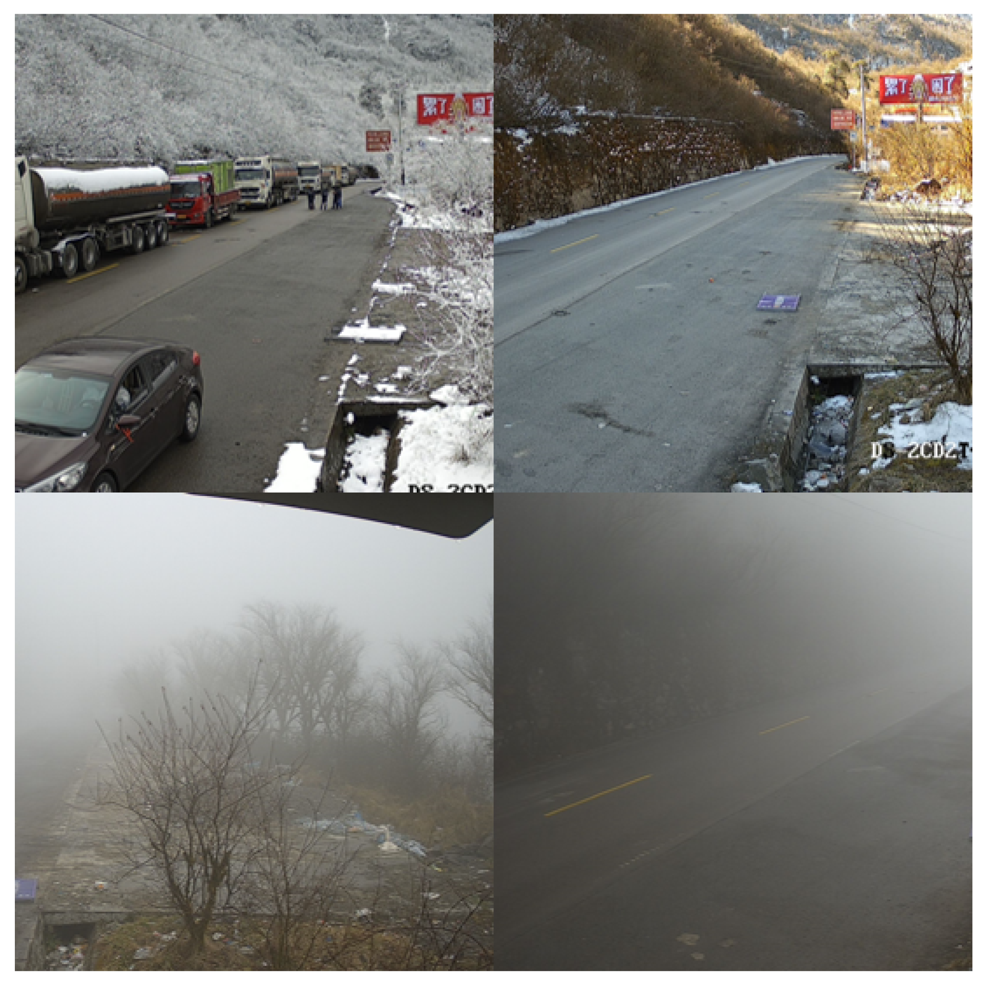
Figure 2.
Diagram of data augmentation with StyleGAN2-ADA.
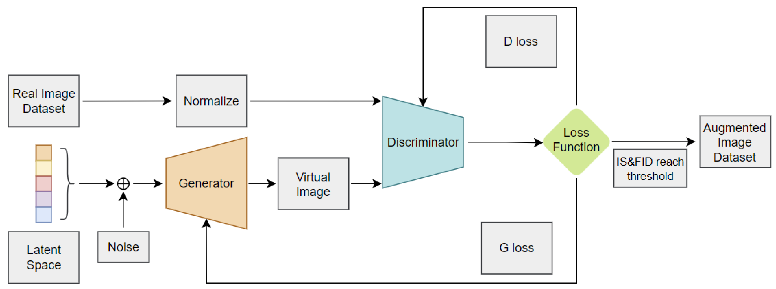
Figure 3.
Composition of the new dataset.
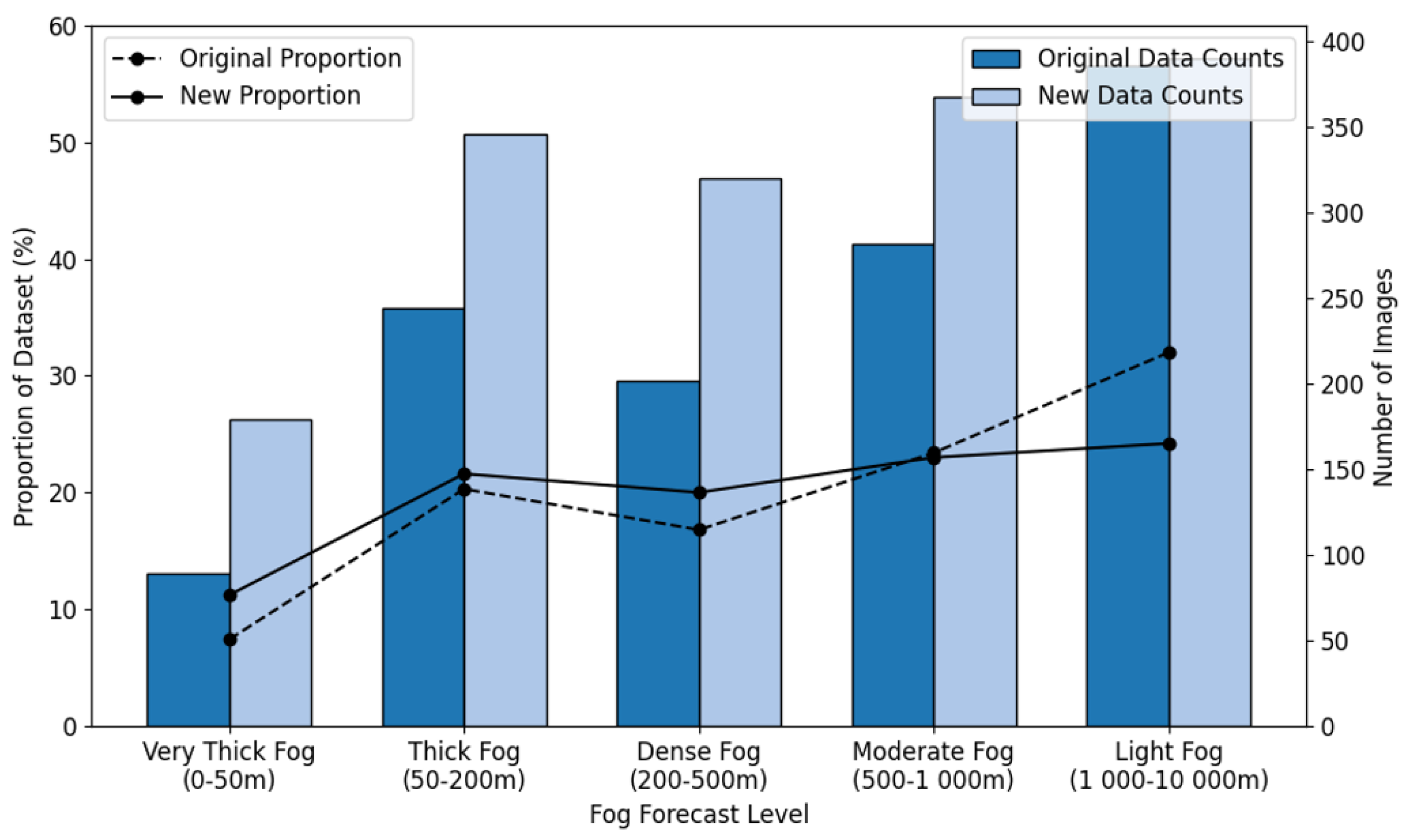
Figure 4.
Foggy images of different fog density: (a) very thick fog, (b) thick fog, (c) dense fog, (d) moderate fog, (e) light fog, and (f) the average normalized features for foggy images of different fog density shown in (a)-(e), respectively.
Figure 4.
Foggy images of different fog density: (a) very thick fog, (b) thick fog, (c) dense fog, (d) moderate fog, (e) light fog, and (f) the average normalized features for foggy images of different fog density shown in (a)-(e), respectively.
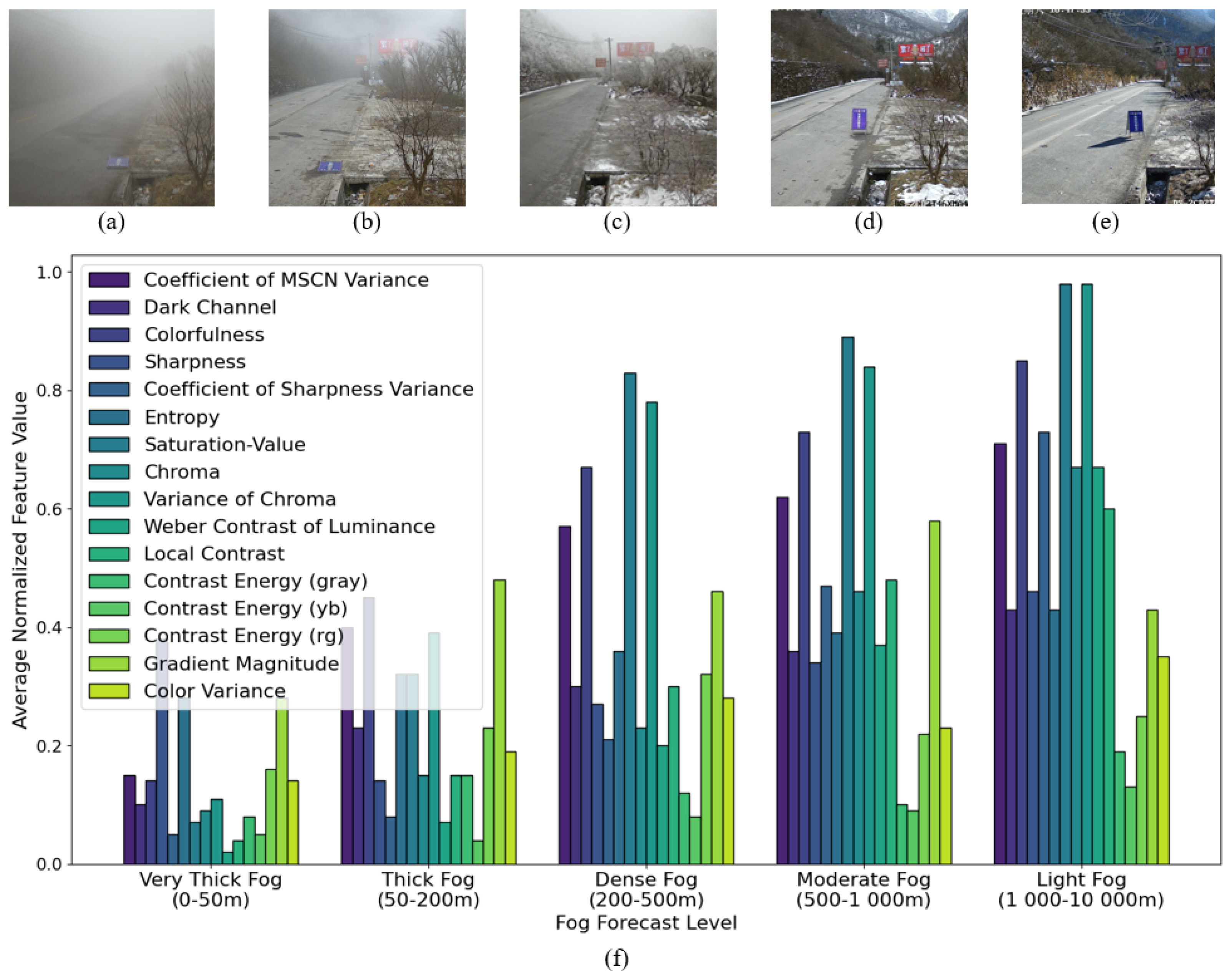
Figure 5.
The correlation coefficient map between features via PCC.
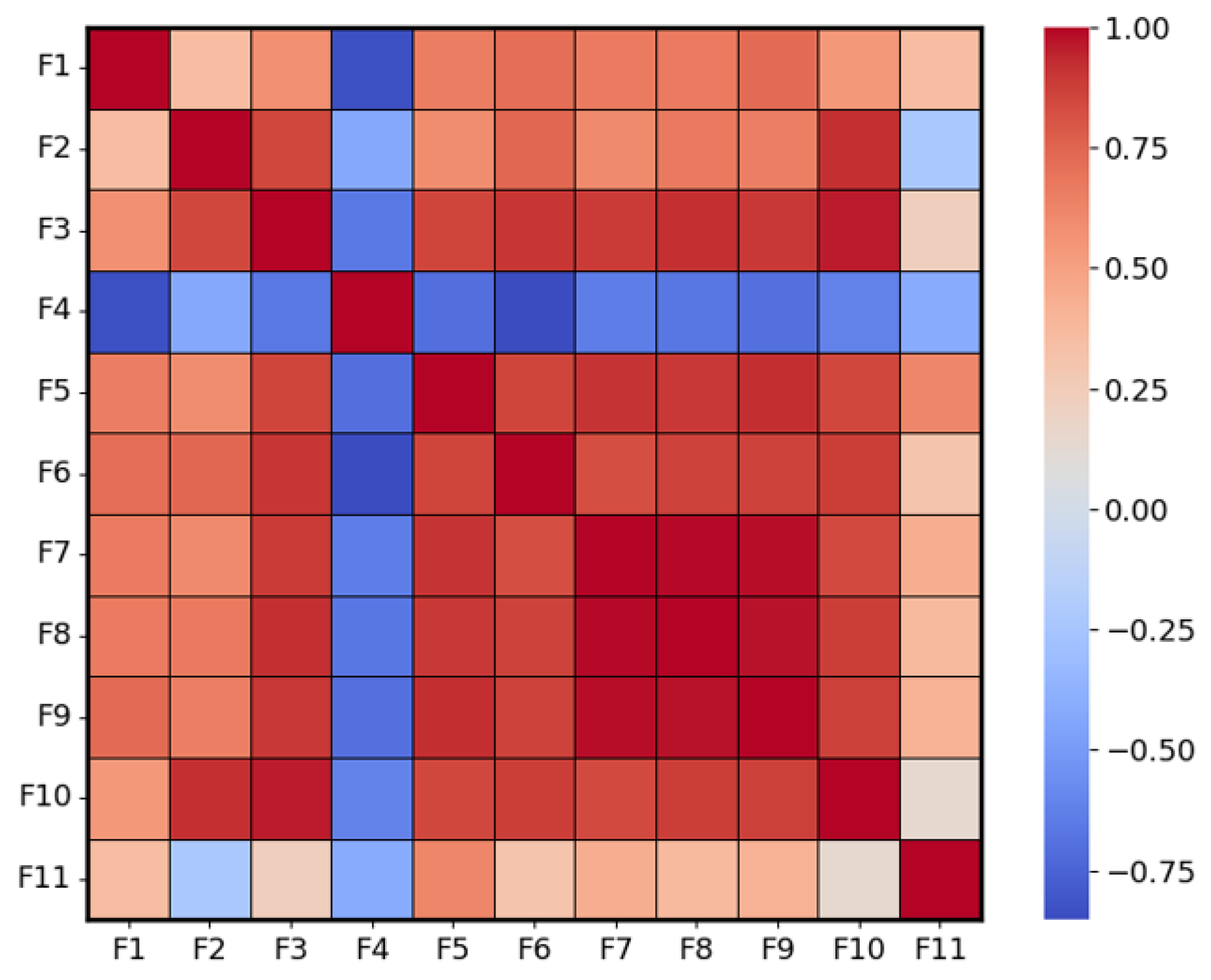
Figure 6.
Training loss variation across different models with respect to the number of iterations.
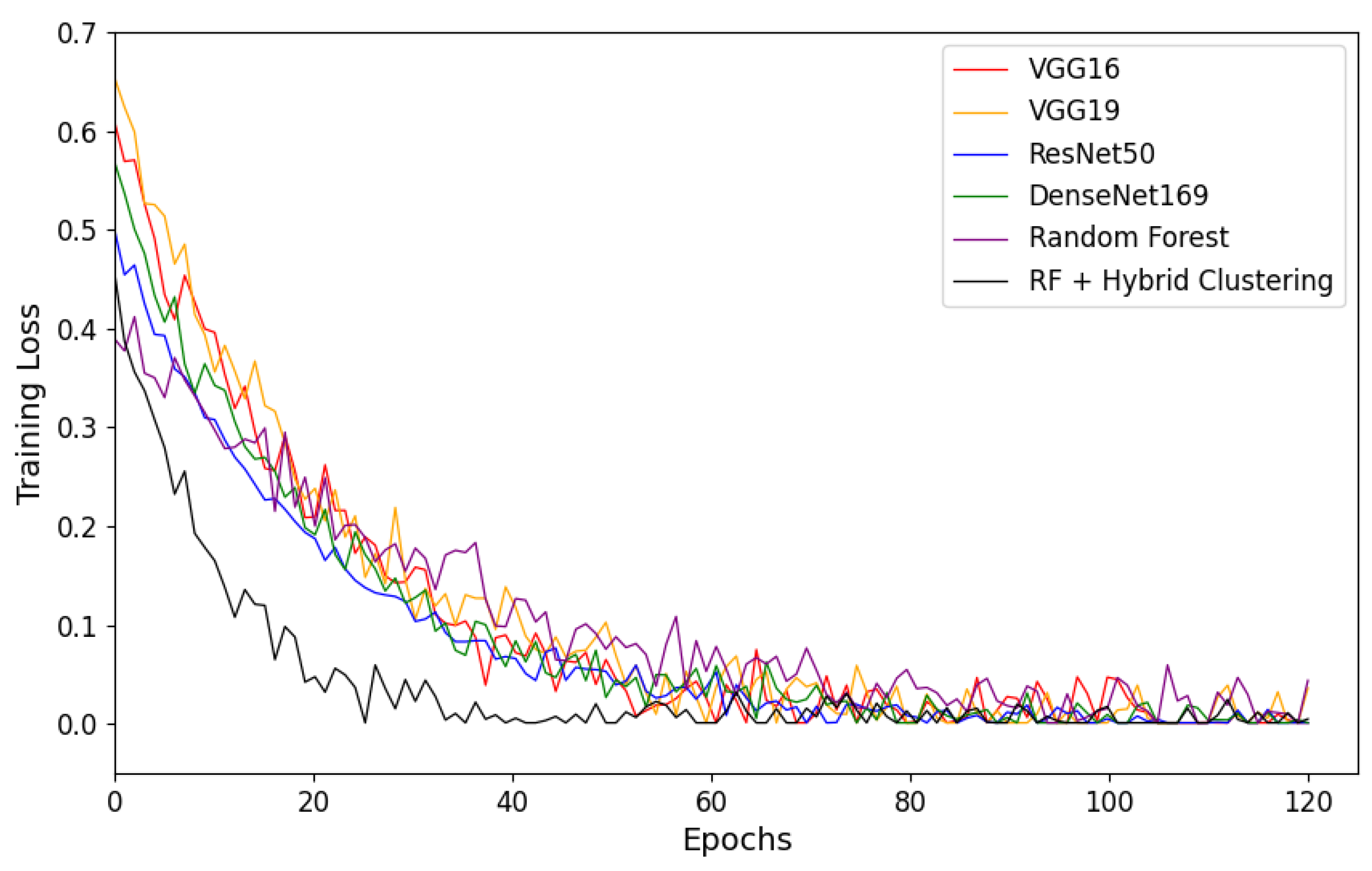

Table 1.
FOG DENSITY.
| Fog Density | Visibility Range |
|---|---|
| Light Fog | |
| Moderate Fog | |
| Dense Fog | |
| Thick Fog | |
| Very Thick Fog |
Table 2.
INCEPTION SCORE AND FID OF GENERATED IMAGES FOR DIFFERENT GRADES.
| 0-50m | 50-200m | 200-500m | 500-1 000m | 1 000-10 000m | Av. | |
|---|---|---|---|---|---|---|
| Inception Score | 3.81 | 3.21 | 4.26 | 3.42 | 3.33 | 3.61 |
| FID value | 98.01 | 98.19 | 98.91 | 93.53 | 92.69 | 96.27 |
Table 3.
CORRELATION COEFFICIENT BETWEEN VISIBILITY RANGE AND ELEVEN FEATURES BY PCC.
| Fog-relevant Features | Serial Number | Correlation Coefficient |
|---|---|---|
| Coefficients of MSCN Variance | F1 | 0.493 |
| Dark channel | F2 | 0.562 |
| Colorfulness | F3 | 0.581 |
| Sharpness | F4 | 0.457 |
| Coefficient of sharpness variance | F5 | 0.477 |
| Entropy | F6 | 0.481 |
| Combination of saturation and value in HSV space | F7 | 0.440 |
| Chroma | F8 | 0.632 |
| Variance of chroma | F9 | 0.534 |
| Weber contrast of luminance | F10 | 0.555 |
| Local contrast | F11 | 0.512 |
| Contrast energy (gray) | F12 | 0.354 |
| Contrast energy (yb) | F13 | 0.313 |
| Contrast energy (rg) | F14 | 0.367 |
| Gradient magnitude | F15 | 0.295 |
| Color variance | F16 | 0.308 |
Table 4.
FOG DENSITY ACCURACY OF DIFFERENT MODELS TRAINED BY ORIGINAL DATA.
| Fog Density | ||||||
|---|---|---|---|---|---|---|
| Very Thick Fog | Thick Fog | Dense Fog | Moderate Fog | Light Fog | Total | |
| VGG-16(%) | 63.2 | 73.3 | 84.1 | 85.5 | 87.7 | 83.9 |
| VGG-19(%) | 64.7 | 71.4 | 84.7 | 86.6 | 86.3 | 85.6 |
| ResNet-50(%) | 68.5 | 76.5 | 85.3 | 88.4 | 90.1 | 86.9 |
| DenseNet-169(%) | 64.7 | 69.3 | 83.4 | 89.6 | 90.1 | 85.8 |
| Random Forest(%) | 55.1 | 68.7 | 83.4 | 88.9 | 90.8 | 84.1 |
| Random Forest based on hybrid clustering(%) | 58.5 | 70.5 | 85.5 | 89.7 | 91.1 | 86.4 |
Table 5.
FOG DENSITY ACCURACY OF DIFFERENT MODELS TRAINED BY AUGMENTED DATA.
| Fog Density | ||||||
|---|---|---|---|---|---|---|
| Very Thick Fog | Thick Fog | Dense Fog | Moderate Fog | Light Fog | Total | |
| VGG-16(%) | 81.3 | 88.3 | 86.1 | 88.5 | 89.7 | 86.2 |
| VGG-19(%) | 82.7 | 86.2 | 89.7 | 90.3 | 91.3 | 89.6 |
| ResNet-50(%) | 83.4 | 89.3 | 91.3 | 89.1 | 90.4 | 88.9 |
| DenseNet-169(%) | 84.3 | 89.6 | 91.4 | 92.6 | 93.6 | 91.2 |
| Random Forest(%) | 89.0 | 92.7 | 91.4 | 89.9 | 92.3 | 90.1 |
| Random Forest based on hybrid clustering(%) | 89.8 | 91.7 | 94.5 | 92.7 | 94.9 | 93.0 |
Table 6.
QUANTITATIVE ANALYSIS FOR IMAGE-BASED ARCHITECTURES.
| Reference | Used Method | Visibility Range (m) | Feature Extractor | Classifier/Regressor | Dataset | Accuracy |
|---|---|---|---|---|---|---|
| Li et al. [12] | Deep learning approach based on the fusion of extracted features from the selected subregions for visibility estimation. | 0-12 000 | VGG-16 | Multi-SVR | HKO (4841 images) | 0.88 |
| Loet al.[13] | PSO-based transfer learning approach for feature selection and Multi-SVR model to estimate visibility. | 10 000-40 000 | VGG-19 DenseNet ResNet_50 VGG-16 VGG-19 DenseNet ResNet_50 | Multi-SVR | Private Dataset (6048 images) | 0.88 0.90 0.91 0.90 0.90 0.91 0.93 |
| Liu et al.[14] | STCN-Net model that combines engineered and learned features. | 50-10 000 | Swin-T + ResNet-18 | Fully Connected | VID I | 0.98 |
| Choi et al. [15] | Detection of daytime sea fog and estimating visibility distance from CCTV images. | 0-20 000 | VGG19 | Fully Connected | Private Dataset (5104 images) | 0.72 |
| Zhanget al.[16] | Estimation of quantified visibility based on physical laws and deep learning architectures. | 0-35 000 | DQVENet | Specific algorithm | QVEData | 0.87 |
Disclaimer/Publisher’s Note: The statements, opinions and data contained in all publications are solely those of the individual author(s) and contributor(s) and not of MDPI and/or the editor(s). MDPI and/or the editor(s) disclaim responsibility for any injury to people or property resulting from any ideas, methods, instructions or products referred to in the content. |
© 2024 by the authors. Licensee MDPI, Basel, Switzerland. This article is an open access article distributed under the terms and conditions of the Creative Commons Attribution (CC BY) license (https://creativecommons.org/licenses/by/4.0/).
Copyright: This open access article is published under a Creative Commons CC BY 4.0 license, which permit the free download, distribution, and reuse, provided that the author and preprint are cited in any reuse.


