This study presents an eco-epidemiological model exploring a prey population infected by two distinct pathogen strains in the presence of an unaffected predator population. The model investigates how prey herding behavior provides protection against predation under multi-strain infections. A well-posedness and boundedness analysis of the populations ensures the robustness of the model. Linear stability analysis reveals that, under specific herd shapes and predator mortality rates, prey infected with either strain can vanish. Bifurcation analysis uncovers critical dynamics: a supercritical Hopf bifurcation occurs at a threshold prey herd shape (k), indicating the onset of stable oscillatory population cycles. As predator mortality (δ) varies, both subcritical and supercritical Hopf bifurcations emerge, marking shifts between stable and unstable dynamics, potentially leading to prey extinction or sharp population collapses. The analysis further identifies a Generalized Hopf bifurcation, distinguishing between predictable cycles and more complex. Numerical simulations confirm these findings, offering insights into predator-prey dynamics in ecosystems subject to multi-strain infections. The results have potential implications for understanding disease control, population stability, and ecological resilience.

Keywords:

Subject: Computer Science and Mathematics - Mathematical and Computational Biology

1. Introduction

Predator-prey dynamics are critical in maintaining ecological balance, influenced by various factors such as resource availability, environmental conditions, and predation efficiency [1,2,3,4]. However, the impact of diseases on these interactions [5,6,7,8,9,10,11], especially multi-strain infections [13] within prey populations, has been less explored [14,24,25,26]. When prey are infected, their ability to evade predators declines, not only due to physical weakening but also through behavioral changes such as the formation of herds. These herds serve as protective mechanisms [21,22,23,30], but in the presence of infection, they can introduce additional complexity to the predator-prey relationship [12,29,31,32,34].

In this study, we develop an eco-epidemiological model that investigates how two distinct strains of pathogens interact with herding behavior in prey populations, while predators remain unaffected by the infections themselves. This multi-strain dynamic introduces nontrivial challenges in understanding population stability and predator efficiency. Through this model, we explore how herd shape and predator mortality rates, driven by the protective behavior of herds, influence disease dynamics and population survival.

The real-world applicability of this model is significant. Wildlife populations such as deer, wild boars, and fish frequently experience multi-strain infections that affect both prey behavior and predator efficiency [35,36]. Similarly, agricultural systems [39], where livestock herds [37,38] encounter various pathogens, offer another layer of complexity. In marine ecosystems, schooling fish serve as prey for larger predators, where infection can compromise their defense mechanisms [41,42,43]. Furthermore, urban wildlife and zoonotic diseases [33,47,48,49,50] provide an additional domain where multi-strain infections and human interaction complicate traditional predator-prey dynamics [44,45,46]. The model thus offers critical insights for managing disease outbreaks, ensuring wildlife conservation, and predicting shifts in population stability under varying environmental conditions.

Some researchers have considered two strains of infection either in prey or predator [24,25,26,27,28] but could not show the coexistence of both strains of infections. Martcheva M. [51] considered two types of model with susceptible and two strain infected prey and one with generalist predator, second with specialist predator. She showed that increasing predation leads to eradication of disease without extinction of prey population and also that the presence of specialist predators may lead to the coexistence of both strains. To our knowledge, no one has studied two strains of infection in prey with prey herd and predator mortality due to prey herd. Here we have also assumed both the strains of infections don’t affect each other. That means there is neither coinfection nor superinfection,i.e. when an individual species gets infected by one strain, it cannot develop the second strain and have both strains of infection at the same time nor the second strain can replace the first strain.

We focus on analyzing the stability of populations through well-posedness and boundedness evaluations. Using bifurcation analysis, we reveal the critical thresholds at which the prey population undergoes significant dynamic shifts—highlighting the occurrence of supercritical and subcritical Hopf bifurcations, and their roles in population oscillations or collapse. This investigation of bifurcations provides valuable insights into how changes in herd formation or predator mortality due to herd protection can trigger these complex behaviors. We show the presence of the limit point bifurcation of limit cycles, emerging from the Generalized Hopf bifurcation point. This study contributes to a deeper understanding of eco-epidemiological interactions involving multiple infection strains and predator-prey dynamics, laying the groundwork for future models that can incorporate additional environmental and behavioral complexities.

2. Mathematical Model Formulation

The system model is formed based on the following assumptions:

The susceptible prey grows logistically in the absence of infected prey and predator and prey infected with both strains neither contribute to the reproduction nor to the carrying capacity thus we have,

$\begin{matrix} S^{'} = r S (1 - \frac{S}{K}) \end{matrix}$

(1)
Infection of both strains within the prey population occurs horizontally via direct contact following the mass action incidence i.e.

$\begin{matrix} H (S, I_{j}) = β_{j} I_{j} S for j = 1, 2 \end{matrix}$

(2)

where $β_{j}$ are the rate of transmission of strain j infection.
Only susceptible prey participates in the herding group where the rate of herd shape is $0 < k < 1$
- if the herd shape is circle or square, $k = 0.5$
- if the herd shape is cube or sphere, $k = 0.67$ .
The infected prey dies out either due to disease by strain 1 or 2 or naturally ( $μ_{j} for j = 1, 2$ denotes the total death rate)and upon recovery( $γ_{j} for j = 1, 2$ denotes the recovery rates) from the infection they re-enter the susceptible population.
Predators attack the susceptible prey according to the Holling-II interaction functional type created by S.Djilali [30] given as

$\begin{matrix} H (S, P) = \frac{a S^{k} P}{1 + a h S^{k}} \end{matrix}$

(3)

and the prey infected with strains 1 and 2 according to the Holling type-I functional response given as

$\begin{matrix} H (I_{j}, P) = β_{j} I_{j} P for j = 1, 2 . \end{matrix}$

(4)
Predators attack the boundary of the herd and the prey on the outer herd can injure the predators leading to their death given as $δ S^{k} P$ .

Using the above postulates, we construct a four-dimensional eco-epidemiological model:

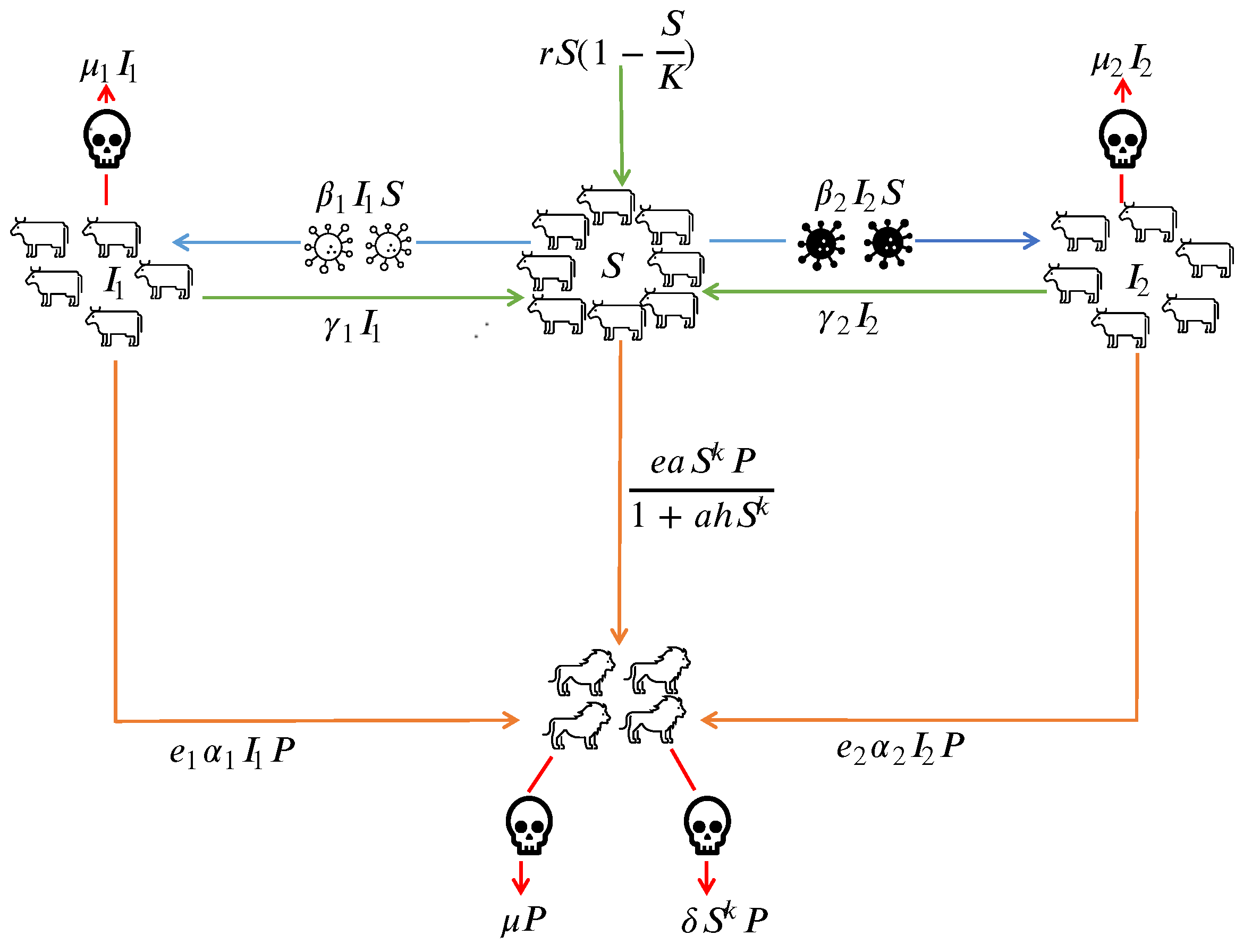
\begin{matrix} \frac{d S}{d t} & = r S (1 - \frac{S}{K}) - [β_{1} I_{1} + β_{2} I_{2}] S + γ_{1} I_{1} + γ_{2} I_{2} - \frac{a S^{k} P}{1 + a h S^{k}} = ϕ_{1} (S, I_{1}, I_{2}, P) \\ \frac{d I_{1}}{d t} & = β_{1} I_{1} S - (γ_{1} + μ_{1}) I_{1} - α_{1} I_{1} P = ϕ_{2} (S, I_{1}, I_{2}, P) \\ \frac{d I_{2}}{d t} & = β_{2} I_{2} S - (γ_{2} + μ_{2}) I_{2} - α_{2} I_{2} P = ϕ_{3} (S, I_{1}, I_{2}, P) \\ \frac{d P}{d t} & = \frac{a e S^{k} P}{1 + a h S^{k}} + e_{1} α_{1} I_{1} P + e_{2} α_{2} I_{2} P - δ S^{k} P - μ P = ϕ_{4} (S, I_{1}, I_{2}, P) \end{matrix}

(5)

we have considered a system of equations describing a prey-predator model with two strains of infection running in prey species and prey group forming a herd against the predator.

In the first equation we assume the logistic growth rate of susceptible prey with r as the intrinsic growth rate and K as carrying capacity. The susceptible prey gets infected by strain 1 and strain 2 with rates of transmission

β_{1}, β_{2}

respectively. The susceptible prey forms a herd and the predator attacks on the boundary of the herd with a Holling type-II interaction functional response.

In the second and third equations, we have the interaction of susceptible prey and the prey infected with strain 1 and strain 2 assuming that the infected can be recovered with rates

γ_{1}, γ_{2}

and join the class of susceptible prey and die with total death rates

μ_{1}, μ_{2}

respectively. Also the predator attacks both the prey infected with strain 1 and strain 2 with linear rates

α_{1}, α_{2}

respectively.

In the fourth equation, we have the growth of predators by consuming susceptible and infected prey with conversion efficiency rates

e, e_{1}, e_{2}

. Also, we have considered the mortality of predators due to prey herd(

δ

) and their natural death(

μ)

Figure 1. Schematic flowchart for the model.

3. Description of Parameters

Parameters	Description

S	Susceptible Prey
$I_{1}$	Prey Infected with strain 1
$I_{2}$	Prey Infected with strain 2
P	Predator
r	Intrinsic growth rate of susceptible prey
K	carrying capacity of susceptible prey
$β_{1}$	rate of transmission of strain 1 infection
$β_{2}$	rate of transmission of strain 2 infection
$γ_{1}$	recovery rate from strain 1
$γ_{2}$	recovery rate from strain 2
a	rate of predation on susceptible prey
k	rate of prey herd shape
h	handling time spent by a predator on healthy prey
$α_{1}$	rate of predation on prey infected with strain 1
$α_{2}$	rate of predation on prey infected with strain 2
e	conversion rate of susceptible prey to predator
$e_{1}$	conversion rate of prey infected with strain 1 to predator
$e_{2}$	conversion rate of prey infected with strain 2 to predator
$δ$	mortality rate of a predator due to prey herd
$μ$	natural death rate of predator
$μ_{1}$	total death rate of prey infected with strain 1
$μ_{2}$	total death rate of prey infected with strain 2

4. Well-Posedness of the Formulated Model

Theorem 1.

All the solutions of the system (5) under the given initial condition are unique and positive in R.

Proof of Theorem 1.

The function

ϕ_{1}, ϕ_{2}, ϕ_{3}

on the right hand side of system of equation(5) are locally Lipschitz Continuous in the region

Υ = {(S, I_{1}, I_{2}, P) \in [ξ, A] \times [0, B] \times [0, B] \times [0, C]}

with

ξ

a positive real constant. This can be seen

\forall S_{1}, S_{2} \in Υ

we have,

\begin{matrix} \begin{matrix} | ϕ_{1} (S_{1}, I_{1}, I_{2}, P) - ϕ_{1} (S_{2}, I_{1}, I_{2}, P) | & \leq r | S_{1} - S_{2} | + \frac{r}{K} | S_{1} - S_{2} | | S_{1} + S_{2} | + (β_{1} | I_{1} | + β_{2} | I_{2} |) | S_{1} - S_{2} | \\ + \frac{a | P | | S_{1}^{k} - S_{2}^{k} | | S_{1} - S_{2} |}{| 1 + a h S_{1}^{k} | | 1 + a h S_{2}^{k} | | S_{1} - S_{2} |} \\ \leq | S_{1} - S_{2} | (. r + \frac{r (| S_{1} | + | S_{2} |)}{K} + β_{1} | I_{1} | + β_{2} | I_{2} | \\ + \frac{a | P |}{| 1 + a h S_{1}^{k} | | 1 + a h S_{2}^{k} |} |\frac{S_{1}^{k} - S_{2}^{k}}{S_{1} - S_{2}}| .) \\ \leq L | S_{1} - S_{2} | \end{matrix} \end{matrix}

where

L = r + \frac{2 r A}{K} + B (β_{1} + β_{2}) + a k C q^{k - 1} > 0

is a Lipschitz constant.

Thus

ϕ_{1} (S, I_{1}, I_{2}, P)

is locally Lipschitz-continuous with respect to S. Similarly, it can be shown for

I_{1}, I_{2}, P

. Hence the system has a unique solution in the region

Υ

Now, to show we have positive solutions, we will show

S (t) > 0 \forall t > 0

by contradiction. Let us assume there exists a

τ > 0

with

τ = i n f {t : S (t) = 0, t > 0}

,such that

\frac{d S}{d t} |_{t = τ} < 0 and S (t) > 0 \forall t \in [0, τ)

. From the first equation of (5) we have,

\begin{matrix} \frac{d S}{d t} |_{t = τ} & = r S (τ) (1 - \frac{S (τ)}{K}) - [β_{1} I_{1} (τ) + β_{2} I_{2} (τ)] S (τ) + γ_{1} I_{1} τ) + γ_{2} I_{2} (τ) - \frac{a S^{k} (τ) P (τ)}{1 + a h S^{k} (τ)} \\ = γ_{1} I_{1} (τ) + γ_{2} I_{2} (τ) \end{matrix}

we can write the second, third, fourth equations of the model (5) as:

\frac{d I_{1}}{d t} = I_{1} f_{1} (S, I_{1}, I_{2}, P), \frac{d I_{2}}{d t} = I_{2} f_{2} (S, I_{1}, I_{2}, P), \frac{d P}{d t} = P f_{3} (S, I_{1}, I_{2}, P)

where

f_{1} (S, I_{1}, I_{2}, P) = β_{1} S - α_{1} P - γ_{1} - μ_{1}

f_{2} (S, I_{1}, I_{2}, P) = β_{2} S - α_{2} P - γ_{2} - μ_{2}

f_{3} (S, I_{1}, I_{2}, P) = \frac{e a S^{k}}{1 + a h S^{k}} + e_{1} α_{1} I_{1} + e_{2} α_{2} I_{2} - δ S^{k} - μ

thus it follows,

I_{1} (t) = I_{1} (0) e^{\int_{0}^{t} f_{1} (S (u), I_{1} (u), I_{2} (u), P (u)) d u} \geq 0

I_{2} (t) = I_{2} (0) e^{\int_{0}^{t} f_{2} (S (u), I_{1} (u), I_{2} (u), P (u)) d u} \geq 0

P (t) = P (0) e^{\int_{0}^{t} f_{3} (S (u), I_{1} (u), I_{2} (u), P (u)) d u} \geq 0

Now we have four cases:

(1) I_{1} (0) = I_{2} (0) = 0

then

I_{1} (t) = I_{2} (t) = 0 \forall t > 0 \Rightarrow I_{1} (τ) = I_{2} (τ) = 0

\Rightarrow \frac{d S}{d t} |_{t = τ} = 0

which contradicts the condition

\frac{d S}{d t} |_{t = τ} < 0

\Rightarrow S (t) > 0 \forall t \geq 0

(2) I_{1} (0) > 0 a n d I_{2} (0) > 0

then

I_{1} (t) > 0 a n d I_{2} (t) > 0 \forall t > 0 \Rightarrow I_{1} (τ) > 0 a n d I_{2} (τ) > 0

\Rightarrow \frac{d S}{d t} |_{t = τ} > 0

which contradicts the condition

\frac{d S}{d t} |_{t = τ} < 0

\Rightarrow S (t) > 0 \forall t \geq 0

Similarly, we can prove for the rest two cases i.e.

I_{1} (0) = 0, I_{2} (0) > 0 and I_{1} (0) > 0, I_{2} (0) = 0

Thus all solutions

(S (t), I_{1} (t), I_{2} (t), P (t))

with the stated initial condition remain positive for

\forall t > 0

. □

Theorem 2.

All solutions of the system (5) beginning in

R_{+}^{4}

stay enclosed in the region

Υ = {(S, I_{1}, I_{2}, P) : 0 < S + I_{1} + I_{2} \leq \frac{{(r + ζ_{1})}^{2} K}{4 r ζ_{1}}, 0 < S + \frac{1}{e} P \leq \frac{{(r + ζ_{2})}^{2} K}{4 r ζ_{2}} + γ_{1} \frac{{(r + ζ_{1})}^{2} K}{4 r ζ_{1} ζ_{2}} + γ_{2} \frac{{(r + ζ_{1})}^{2} K}{4 r ζ_{1} ζ_{2}}

, where

ζ_{1} and ζ_{2}

are some real numbers satisfying

0 < ζ_{1} < m i n {μ_{1}, μ_{2}}, 0 < ζ_{2} < μ - \frac{(e_{1} α_{1} + e_{2} α_{2}) {(r + ζ_{1})}^{2} K}{4 r ζ_{1}}

Proof of Theorem 2.

From the first equation of the system, we have

lim_{t \to \infty} \sup S (t) \leq K .

Let

ϕ_{1} = S + I_{1} + I_{2}

and

ζ_{1} > 0

. Then

\begin{matrix} \begin{matrix} \frac{d ϕ_{1}}{d t} + ζ_{1} ϕ_{1} & = r S (1 - \frac{S}{K}) - \frac{a S^{k} P}{1 + a h S^{k}} - α_{1} I_{1} P - α_{2} I_{2} P - μ_{1} I_{1} - μ_{2} I_{2} + ζ_{1} (S + I_{1} + I_{2}) \\ \leq r S (1 - \frac{S}{K}) - μ_{1} I_{1} - μ_{2} I_{2} + ζ_{1} (S + I_{1} + I_{2}) \\ \leq (r + ζ_{1}) S - \frac{r S^{2}}{K} - (μ_{1} - ζ_{1}) I_{1} - (μ_{2} - ζ_{1}) I_{2} \\ \leq (r + ζ_{1}) S - \frac{r S^{2}}{K}, for ζ_{1} < m i n {μ_{1}, μ_{2}} \end{matrix} \end{matrix}

since

max_{S \geq 0} (r + ζ_{1}) S - \frac{r S^{2}}{K} = \frac{{(r + ζ_{1})}^{2} K}{4 r}

Therefore,

\frac{d ϕ_{1}}{d t} + ζ_{1} ϕ_{1} \leq \frac{{(r + ζ_{1})}^{2} K}{4 r} \Rightarrow lim_{t \to \infty} \sup (S (t) + I_{1} (t) + I_{2} (t)) \leq \frac{{(r + ζ_{1})}^{2} K}{4 r ζ_{1}}

Now, to check boundedness of

P (t)

we assume

ϕ_{2} = S + \frac{1}{e} P

and

ζ_{2} > 0

. Then

\begin{matrix} \begin{matrix} \frac{d ϕ_{2}}{d t} + ζ_{2} ϕ_{2} & = r S (1 - \frac{S}{K}) - β_{1} I_{1} S - β_{2} I_{2} S + γ_{1} I_{1} + γ_{2} I_{2} + \frac{e_{1}}{e} α_{1} I_{1} P + \frac{e_{2}}{e} α_{2} I_{2} P \\ - \frac{δ}{e} S^{k} P - \frac{μ}{e} P + ζ_{2} S + \frac{ζ_{2}}{e} P \\ \leq (r + ζ_{2}) S - \frac{r S^{2}}{K} + γ_{1} I_{1 m a x} + γ_{2} I_{2 m a x} - (\frac{μ}{e} - \frac{ζ_{2}}{e} - \frac{e_{1}}{e} α_{1} I_{1 m a x} - \frac{e_{2}}{e} α_{2} I_{2 m a x}) P \end{matrix} \end{matrix}

where

I_{1 m a x} = I_{2 m a x} = \frac{{(r + ζ_{1})}^{2} K}{4 r ζ_{1}}

Now for

0 < ζ_{2} < μ - e_{1} α_{1} I_{1 m a x} - e_{2} α_{2} I_{2 m a x}

, we have

\frac{d ϕ_{2}}{d t} + ζ_{2} ϕ_{2} \leq (r + ζ_{2}) S - \frac{r S^{2}}{K} + γ_{1} I_{1 m a x} + γ_{2} I_{2 m a x}

which implies

lim_{t \to \infty} \sup (S (t) + \frac{1}{e} P (t)) \leq \frac{{(r + ζ_{2})}^{2} K}{4 r ζ_{2}} + γ_{1} \frac{{(r + ζ_{1})}^{2} K}{4 r ζ_{1} ζ_{2}} + γ_{2} \frac{{(r + ζ_{1})}^{2} K}{4 r ζ_{1} ζ_{2}}

Hence the theorem follows. □

5. Equilibrium Points

The model system (5) has following feasible equilibrium points:

$E_{1} = (0, 0, 0, 0)$
$E_{2} = (K, 0, 0, 0)$

The basic reproduction number at the disease-free equilibrium point is

$R_{0} = m a x {R_{0}^{1}, R_{0}^{2}}$ where $R_{0}^{1} = \frac{β_{1} K}{γ_{1} + μ_{1}}, R_{0}^{2} = \frac{β_{2} K}{γ_{2} + μ_{2}}$
$E_{3} = (S_{S P}, 0, 0, P_{S P})$

where $S_{S P} and P_{S P}$ are solutions of equations:

$a h δ S^{2 k} + S^{k} (δ + μ a h - a e) + μ = 0$ and $r S (1 - \frac{S}{K}) - \frac{a S^{k} P}{1 + a h S^{k}} = 0$

For positive solutions, the following conditions should hold:

${(μ a h + δ - a e)}^{2} \geq 4 a h δ μ$ and $δ + μ a h < a e$
$E_{4} = (S_{1}, I_{1}, 0, 0)$

where $S = \frac{μ_{1} + γ_{1}}{β_{1}}, I_{1} = \frac{r S}{μ_{1}} (1 - \frac{S}{K})$
$E_{5} = (S_{2}, 0, I_{2}, 0)$

where $S = \frac{μ_{2} + γ_{2}}{β_{2}}, I_{2} = \frac{r S}{μ_{2}} (1 - \frac{S}{K})$
$E_{6} = (S_{I_{1} P}, I_{1}, 0, P)$

where $I_{1} = \frac{1}{e_{1} α_{1}} (δ S^{k} + μ - \frac{e a S^{k}}{1 + a h S^{k}})$ , $P = \frac{β_{1} S - γ_{1} - μ_{1}}{α_{1}}$

$f_{1} (S) = A_{1} S^{2 k + 1} + A_{2} S^{2 k} + A_{3} S^{k + 2} + A_{4} S^{k + 1} + A_{5} S^{k} + A_{6} S^{2} + A_{7} S + A_{8}$

$\begin{matrix} where A_{1} = δ a h K β_{1}, A_{2} = - δ a h γ_{1} K, A_{3} = a h r e_{1} α_{1}, A_{4} = β_{1} e_{1} a K - a e K β_{1} + K β_{1} δ + μ a h K β_{1} - r e_{1} α_{1} a h K, \\ A_{5} = a e γ_{1} K - δ γ_{1} K - μ a h γ_{1} K - (γ_{1} + μ_{1}) e_{1} a K, A_{6} = r e_{1} α_{1}, A_{7} = K (μ β_{1} - r e_{1} α_{1}), A_{8} = - μ γ_{1} K \end{matrix}$
$E_{7} = (S_{I_{2} P}, 0, I_{2}, P)$

where $I_{1} = \frac{1}{e_{2} α_{2}} (δ S^{k} + μ - \frac{e a S^{k}}{1 + a h S^{k}})$ , $P = \frac{β_{2} S - γ_{2} - μ_{2}}{α_{2}}$

$f_{2} (S) = A_{1} S^{2 k + 1} + A_{2} S^{2 k} + A_{3} S^{k + 2} + A_{4} S^{k + 1} + A_{5} S^{k} + A_{6} S^{2} + A_{7} S + A_{8}$

$\begin{matrix} where A_{1} = δ a h K β_{2}, A_{2} = - δ a h γ_{2} K, A_{3} = a h r e_{2} α_{2}, A_{4} = β_{2} e_{2} a K - a e K β_{2} + K β_{2} δ + μ a h K β_{2} - r e_{2} α_{2} a h K, \\ A_{5} = a e γ_{2} K - δ γ_{2} K - μ a h γ_{2} K - (γ_{2} + μ_{2}) e_{2} a K, A_{6} = r e_{2} α_{2}, A_{7} = K (μ β_{2} - r e_{2} α_{2}), A_{8} = - μ γ_{2} K . \end{matrix}$
$E^{*} = (S^{*}, I_{1}^{*}, I_{2}^{*}, P^{*})$ where $P^{*} = \frac{β_{1} S - μ_{1} - γ_{1}}{α_{1}} = \frac{β_{2} S - μ_{2} - γ_{2}}{α_{2}}$

$\Rightarrow S^{*} = \frac{α_{2} (μ_{1} + γ_{1}) - α_{1} (μ_{2} + γ_{2})}{β_{1} α_{2} - α_{1} β_{2}}$

$\begin{matrix} I_{1}^{*} & = \frac{K α_{1} (γ_{2} - β_{2} S) (δ S^{k} + μ + a h δ S^{2 k} + μ a h S^{k} - a e S^{k}) - e_{2} α_{2} (β_{1} a K S^{k + 1}) + e_{2} α_{2} (μ_{1} + γ_{1}) K a S^{k} + e_{2} α_{2} α_{1} r S (1 + a h S^{k}) (K - S)}{K α_{1} (1 + a h S^{k}) (e_{1} α_{1} (γ_{2} - β_{2} S) - e_{2} α_{2} (γ_{1} - β_{1} S))} \\ I_{2}^{*} & = \frac{K α_{1} (γ_{1} - β_{1} S) (δ S^{k} + μ + a h δ S^{2 k} + μ a h S^{k} - a e S^{k}) - e_{1} α_{1} (β_{1} a K S^{k + 1}) + e_{1} α_{1} (μ_{1} + γ_{1}) K a S^{k} + e_{1} α_{1}^{2} r S (1 + a h S^{k}) (K - S)}{K α_{1} (1 + a h S^{k}) (e_{2} α_{2} (γ_{1} - β_{1} S) - e_{1} α_{1} (γ_{2} - β_{2} S))} \end{matrix}$

6. Stability Conditions

$E_{1} (0, 0, 0, 0)$ is a saddle point because the eigenvalues of variational matrix are

$(r, - γ_{1} - μ_{1}, - γ_{2} - μ_{2}, - m)$
$E_{2} (K, 0, 0, 0)$ is locally asymptotically stable if

$\frac{K^{k} a e}{K^{k} a h + 1} < K^{k} d + m$ and $K β_{1} < μ_{1} + γ_{1}$ and $K β_{2} < μ_{2} + γ_{2}$
for $E^{*}$ the variational matrix is

$\begin{matrix} J = [\begin{matrix} J_{11} & J_{12} & J_{13} & J_{14} \\ J_{21} & J_{22} & J_{23} & J_{24} \\ J_{31} & J_{32} & J_{33} & J_{34} \\ J_{41} & J_{42} & J_{43} & J_{44} \end{matrix}] \end{matrix}$

where $J_{11} = \frac{a^{2} h k S^{* (2 k - 1)} P^{*}}{{(1 + a h S^{* k})}^{2}} - β_{2} I_{2}^{*} + r (1 - \frac{S^{*}}{K}) - \frac{r S^{*}}{K} - \frac{a k S^{* (k - 1)} P^{*}}{1 + a h S^{* k}} - β_{1} I_{1}^{*}$

$J_{12} = γ_{1} - β_{1} S^{*}$ , $J_{13} = γ_{2} - β_{2} S^{*}$ , $J_{14} = - \frac{a S^{* k}}{1 + a h S^{* k}}$

$J_{21} = β_{1} I_{1}^{*}$ , $J_{22} = β_{1} S^{*} - μ_{1} - α_{1} P^{*} - γ_{1}$ , $J_{23} = 0$ , $J_{24} = - α_{1} I_{1}^{*}$

$J_{31} = β_{2} I_{2}^{*}$ , $J_{32} = 0$ , $J_{33} = β_{2} S^{*} - μ_{2} - α_{2} P^{*} - γ_{2}$ , $J_{34} = - α_{2} I_{2}^{*}$

$J_{41} = \frac{a e k S^{* (k - 1)} P^{*}}{1 + a h S^{* k}} - d k S^{* (k - 1)} P^{*} - \frac{a^{2} e h k S^{* (2 k - 1)} P^{*}}{{(1 + a h S^{* k})}^{2}}$

$J_{42} = α_{1} e_{1} P^{*}$ , $J_{43} = α_{2} e_{2} P^{*}$

$J_{44} = α_{1} e_{1} I_{1}^{*} - d S^{* k} - m + α_{2} e_{2} I_{2}^{*} + \frac{a e S^{* k}}{1 + a h S^{* k}}$

The characteristic polynomial of matrix J is

$λ^{4} + a_{1} λ^{3} + a_{2} λ^{2} + a_{3} λ + a_{4} = 0$

(6)

where

$\begin{matrix} a_{1} & = - (J_{11} + J_{22} + J_{33} + J_{44}) \\ a_{2} & = J_{11} J_{22} - J_{12} J_{21} + J_{11} J_{33} - J_{13} J_{31} + J_{11} J_{44} - J_{14} J_{41} + J_{22} J_{33} - J_{23} J_{32} + J_{22} J_{44} - J_{24} J_{42} + J_{33} J_{44} - J_{34} J_{43} \\ a_{3} & = J_{11} J_{23} J_{32} - J_{11} J_{22} J_{33} + J_{12} J_{21} J_{33} - J_{12} J_{23} J_{31} - J_{13} J_{21} J_{32} + J_{13} J_{22} J_{31} - J_{11} J_{22} J_{44} + J_{11} J_{24} J_{42} + J_{12} J_{21} J_{44} \\ - J_{12} J_{24} J_{41} - J_{14} J_{21} J_{42} + J_{14} J_{22} J_{41} - J_{11} J_{33} J_{44} + J_{11} J_{34} J_{43} + J_{13} J_{31} J_{44} - J_{13} J_{34} J_{41} - J_{14} J_{31} J_{43} + J_{14} J_{33} J_{41} \\ - J_{22} J_{33} J_{44} + J_{22} J_{34} J_{43} + J_{23} J_{32} J_{44} - J_{23} J_{34} J_{42} - J_{24} J_{32} J_{43} + J_{24} J_{33} J_{42} \\ a_{4} & = J_{11} J_{22} J_{33} J_{44} - J_{11} J_{22} J_{34} J_{43} - J_{11} J_{23} J_{32} J_{44} + J_{11} J_{23} J_{34} J_{42} + J_{11} J_{24} J_{32} J_{43} - J_{11} J_{24} J_{33} J_{42} - J_{12} J_{21} J_{33} J_{44} \\ + J_{12} J_{21} J_{34} J_{43} + J_{12} J_{23} J_{31} J_{44} - J_{12} J_{23} J_{34} J_{41} - J_{12} J_{24} J_{31} J_{43} + J_{12} J_{24} J_{33} J_{41} + J_{13} J_{21} J_{32} J_{44} - J_{13} J_{21} J_{34} J_{42} \\ - J_{13} J_{22} J_{31} J_{44} + J_{13} J_{22} J_{34} J_{41} + J_{13} J_{24} J_{31} J_{42} - J_{13} J_{24} J_{32} J_{41} - J_{14} J_{21} J_{32} J_{43} + J_{14} J_{21} J_{33} J_{42} + J_{14} J_{22} J_{31} J_{43} \\ - J_{14} J_{22} J_{33} J_{41} - J_{14} J_{23} J_{31} J_{42} + J_{14} J_{23} J_{32} J_{41} \end{matrix}$

According to Routh-Hurwitz criteria $E^{*}$ is locally asymptotically stable if and only if

$a_{1} > 0, a_{4} > 0, a_{1} a_{2} - a_{3} > 0, a_{1} a_{2} a_{3} - a_{3}^{2} - a_{4} a_{1}^{2} > 0$

Theorem 3.

The necessary and sufficient conditions for Hopf bifurcation to occur at

E^{*}

k = k^{*}

are the following:

$a_{1} > 0, a_{4} > 0, a_{1} a_{2} - a_{3} > 0$
$a_{1} a_{2} a_{3} - a_{3}^{2} - a_{4} a_{1}^{2} = 0$
$a_{1}^{2} (k^{*}) (a_{2} {(k^{*})}^{'} a_{3} (k^{*}) + a_{2} (k^{*}) a_{3}^{'} (k^{*}) - a_{4}^{'} (k^{*}) a_{1} (k^{*})) - 2 a_{3} (k^{*}) a_{3}^{'} (k^{*}) a_{1} (k^{*}) + a_{1}^{'} (k^{*}) (a_{2} (k^{*}) a_{3} (k^{*}) a_{1} (k^{*}) + 2 a_{3}^{2} (k^{*})) \neq 0$

Proof of Theorem 3.

k = k^{*}

the characteristic equation (6)becomes

(λ^{2} (k) + \frac{a_{3} (k)}{a_{1} (k)}) (λ (k) + x_{1} (k)) (λ (k) + x_{2} (k)) = 0

(7)

where

x_{1} + x_{2} = a_{1}, x_{1} x_{2} = a_{2} - \frac{a_{3}}{a_{1}}

Now to show the transversality condition for Hopf-bifurcation. Let us assume

λ (k) = u (k) + i v (k)

. Substituting this in (7) we have,

\begin{matrix} D (k) u {(k)}^{'} - E (k) v {(k)}^{'} + G (k) & = 0 \end{matrix}

(8)

\begin{matrix} E (k) u {(k)}^{'} + D (k) v {(k)}^{'} + H (k) & = 0 \end{matrix}

(9)

where

\begin{matrix} D (k) & = 4 u^{3} (k) - 12 u (k) v^{2} (k) + 3 u^{2} (k) a_{1} (k) - 3 a_{1} (k) v^{2} (k) + 2 a_{2} (k) u (k) + a_{3} (k) \\ E (k) & = 12 u^{2} (k) v (k) - 4 v^{3} (k) + 6 u (k) v (k) a_{1} (k) + 2 a_{2} (k) v (k) \\ G (k) & = a_{1}^{'} (k) (u^{3} (k) - 3 u (k) v^{2} (k)) + a_{2}^{'} (k) (u^{2} (k) - v^{2} (k)) + a_{3}^{'} (k) u (k) + a_{4}^{'} (k) \\ H (k) & = a_{1}^{'} (k) (3 u^{2} (k) v (k) - v^{3} (k)) + a_{3}^{'} (k) v (k) + 2 a_{2}^{'} (k) u (k) v (k) \end{matrix}

Now at

k = k^{*}, u (k^{*}) = 0, v (k^{*}) = \sqrt{\frac{a_{3}}{a_{1}}}

Hence we have,

\begin{matrix} D (k^{*}) & = a_{3} (k^{*}) - 3 a_{1} (k^{*}) v^{2} (k^{*}) = - 2 a_{3} (k^{*}) \\ E (k^{*}) & = 2 a_{2} (k^{*}) v (k^{*}) - 4 v^{3} (k^{*}) = 2 v (k^{*}) (a_{2} (k^{*}) - 2 \frac{a_{3} (k^{*})}{a_{1} (k^{*})}) \\ G (k^{*}) & = a_{4}^{'} (k^{*}) - a_{2}^{'} (k^{*}) v^{2} (k^{*}) = a_{4}^{'} (k^{*}) - a_{2}^{'} (k^{*}) \frac{a_{3} (k^{*})}{a_{1} (k^{*})} \\ H (k^{*}) & = a_{3}^{'} (k^{*}) v (k^{*}) - v^{3} (k^{*}) a_{1}^{'} (k^{*}) = v (k^{*}) (a_{3}^{'} (k^{*}) - a_{1}^{'} (k^{*}) \frac{a_{3} (k^{*})}{a_{1} (k^{*})}) \end{matrix}

On solving (8) and (9) using Cramer’s rule for

u^{'} (k^{*})

we get

\begin{matrix} {[\frac{d R e (λ (k))}{d k}]}_{k = k^{*}} & = u^{'} (k^{*}) \\ = - \frac{G (k^{*}) D (k^{*}) + H (k^{*}) E (k^{*})}{D^{2} (k^{*}) + E^{2} (k^{*})} \\ = - \frac{2 a_{3} (k^{*})}{a_{1} (k^{*})} \frac{M}{D^{2} (k^{*}) + E^{2} (k^{*})} \neq 0 \end{matrix}

provided

M \neq 0

where

M = a_{1}^{2} (k^{*}) (a_{2} {(k^{*})}^{'} a_{3} (k^{*}) + a_{2} (k^{*}) a_{3}^{'} (k^{*}) - a_{4}^{'} (k^{*}) a_{1} (k^{*})) - 2 a_{3} (k^{*}) a_{3}^{'} (k^{*}) a_{1} (k^{*}) + a_{1}^{'} (k^{*}) (a_{2} (k^{*}) a_{3} (k^{*}) a_{1} (k^{*}) + 2 a_{3}^{2} (k^{*}))

Hence the theorem follows. □

7. Numerical Simulation

We first search the equilibrium conditions at parameter values given in the Table 1. The corresponding interior equilibrium point

E^{*} = (16.1282, 3.1825, 0.9785, 0.3282)

with eigenvalues (

- 0.0036 \pm 0.2189 i

- 0.0754

- 0.0132

). We have focused on the behavior of two types of infection within the prey population. First, we show the time series of the two infections under consideration in Figure 2 for the homogeneous distribution of the prey, which shows there is no impact of the herd here. However, we observe that due to the higher recovery and death rates of infection

I_{1}

compared to

I_{2}

, the prevalence of

I_{1}

decays sharply. Consequently, the other variables also stabilize, reaching a steady state. A similar behavior can be expected if the recovery and death rates of

I_{2}

were higher than those of

I_{1}

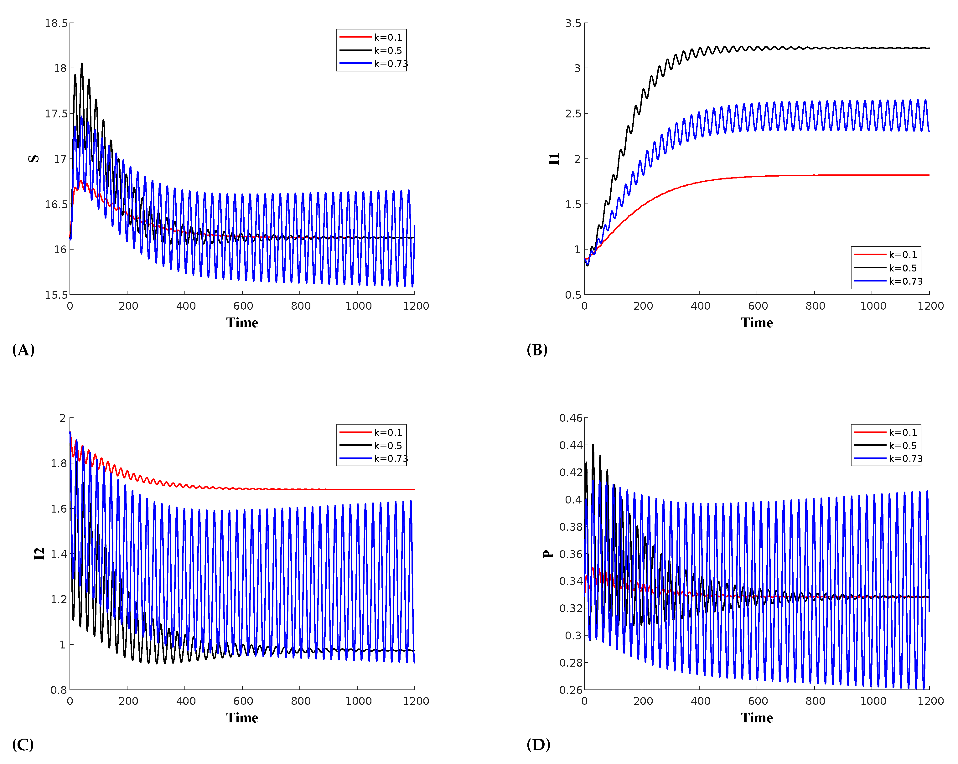
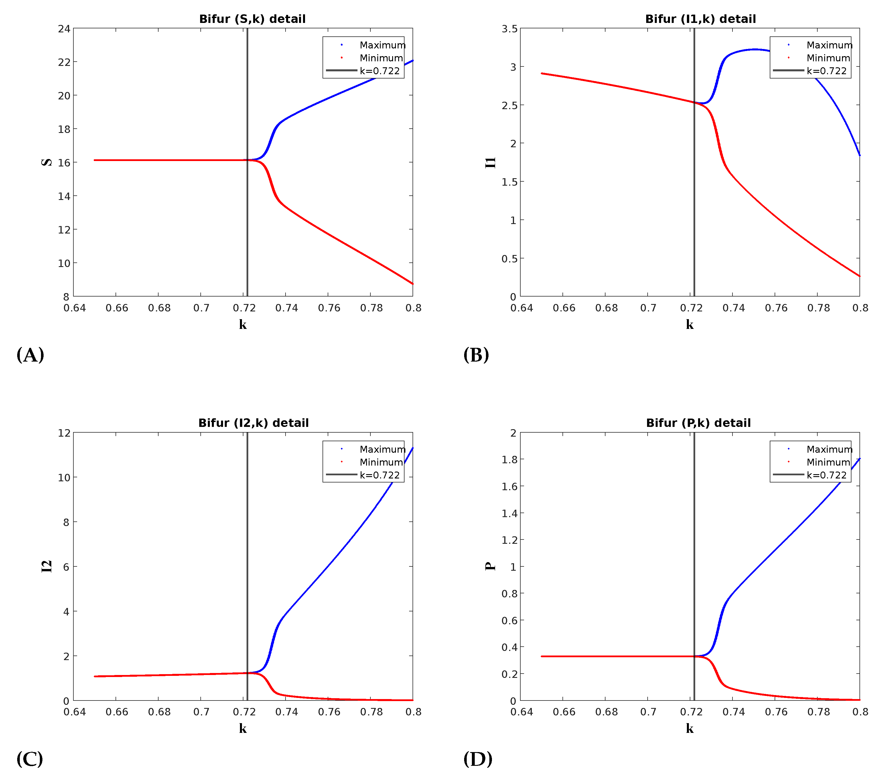
(a) Effect of prey herd shape(k): At

k = 1

, the prey distribution is homogeneous. The value of k reflects the herd shape of the prey, with higher values corresponding to more structured forms, such as cubes or spheres. For instance,

k = 0.67

represents a more defined shape like a sphere or cube, while

k = 0.5

depicts a 2D circular or square herd configuration. Figure 3 illustrates the occurrence of a Hopf bifurcation within this parameter space at

k = 0.722467

, keeping all the other parameters as in Table 1. The first Lyapunov coefficient(FLC) at this point is

- 1.914324 \times 10^{- 4}

which is negative thus confirming supercritical Hopf bifurcation. For the bifurcation analysis a numerical continuation bifurcation package MatCont has been used [52]. The periodic oscillations in the predator populations show that for lower values of k, the predator population decreases. As we increase the value of k, the population decay slows and eventually reaches stable limit cycles at the Hopf bifurcation point. However, we can observe a switching mechanism in the prey population with respect to strain 1. When

I_{1}

is high,

I_{2}

is low, and vice versa. Therefore, as

I_{2}

decays during oscillations,

I_{1}

increases and then decays, but eventually stabilizes at a higher value, while the

I_{2}

infection dies out over time.

Table 1. Parameter Description.

Parameters	Numerical Values	Source
r	0.15	Assumed
K	25	Assumed
$β_{1}$	0.01	[6]
$β_{2}$	0.02	[6]
$γ_{1}$	0.03	[6]
$γ_{2}$	0.01	Assumed
a	0.5	[7]
k	0.55	[7]
h	2	[7]
$α_{1}$	0.15625	Assumed
$α_{2}$	0.8	Assumed
e	0.85	[7]
$e_{1}$	0.17	[7]
$e_{2}$	0.17	[7]
$δ$	0.0145	[7]
$μ$	0.5	[7]
$μ_{1}$	0.08	Assumed
$μ_{2}$	0.05	[7]

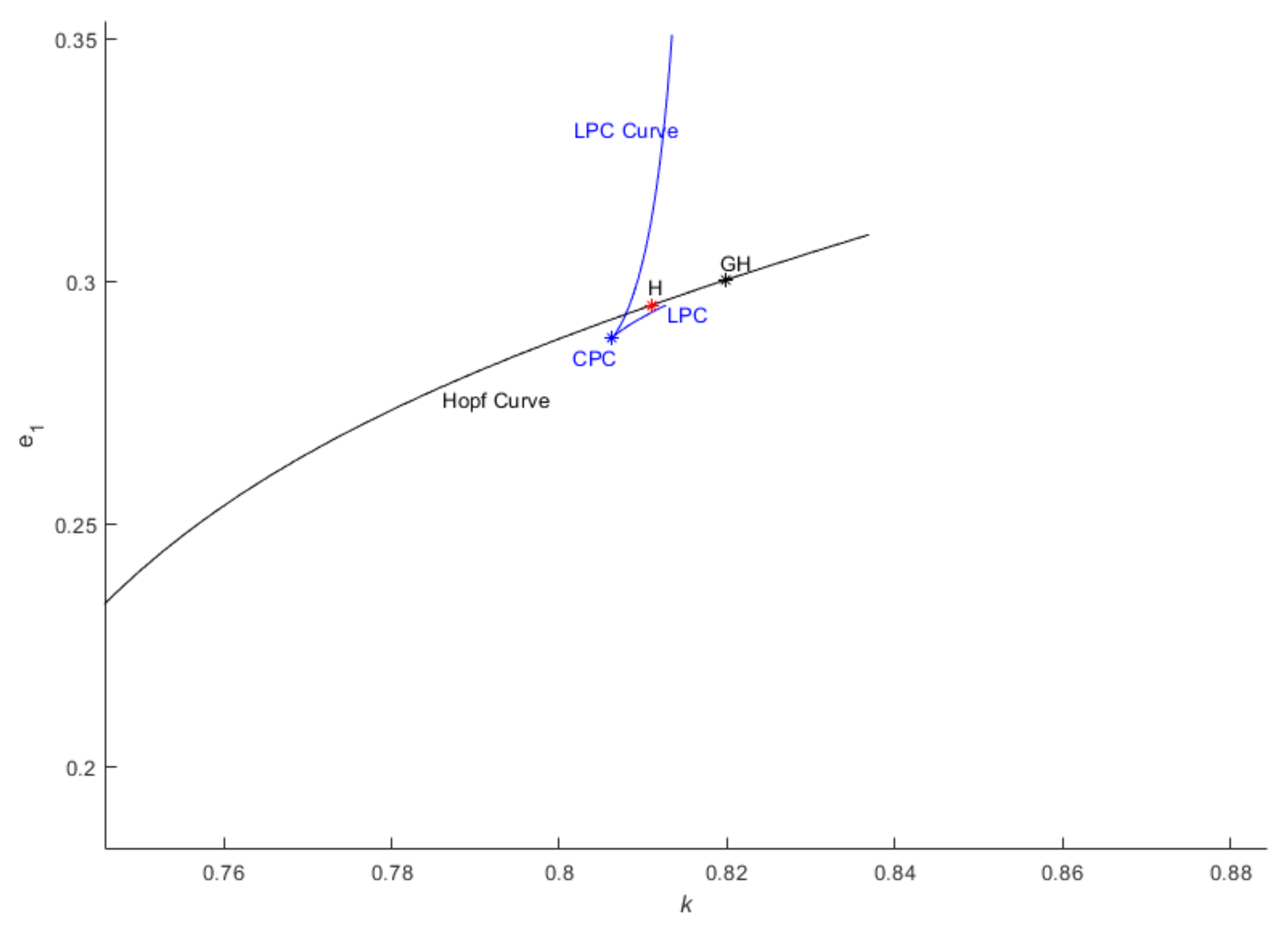
As we have observed the supercritical Hopf bifurcation, we attempt to identify the subcritical Hopf bifurcation in the

k - e_{1}

parametric space. The occurrence of a subcritical Hopf bifurcation is particularly interesting due to the existence of an unstable limit cycle within the linearly stable region [15,16,17,18,19,20]. The demarcation point between the subcritical and supercritical Hopf bifurcations is the Generalized Hopf bifurcation point, which can be reached through the simultaneous variation of two parameters like

k - e_{1}

here. In Figure 5, we have identified the Generalized Hopf bifurcation which is a codimension-2 bifurcation of fixed point, from which a limit point bifurcation of the limit cycle curve (LPC curve) emerges. In this bifurcation, the unstable limit cycle folds into a stable limit cycle of higher amplitude. This LPC curve is also referred to as the global stability boundary by Pandey et al. [15,16]

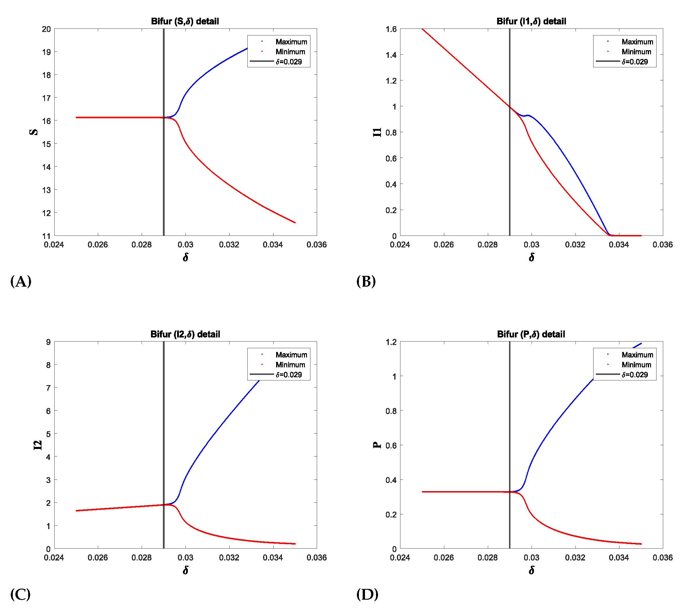
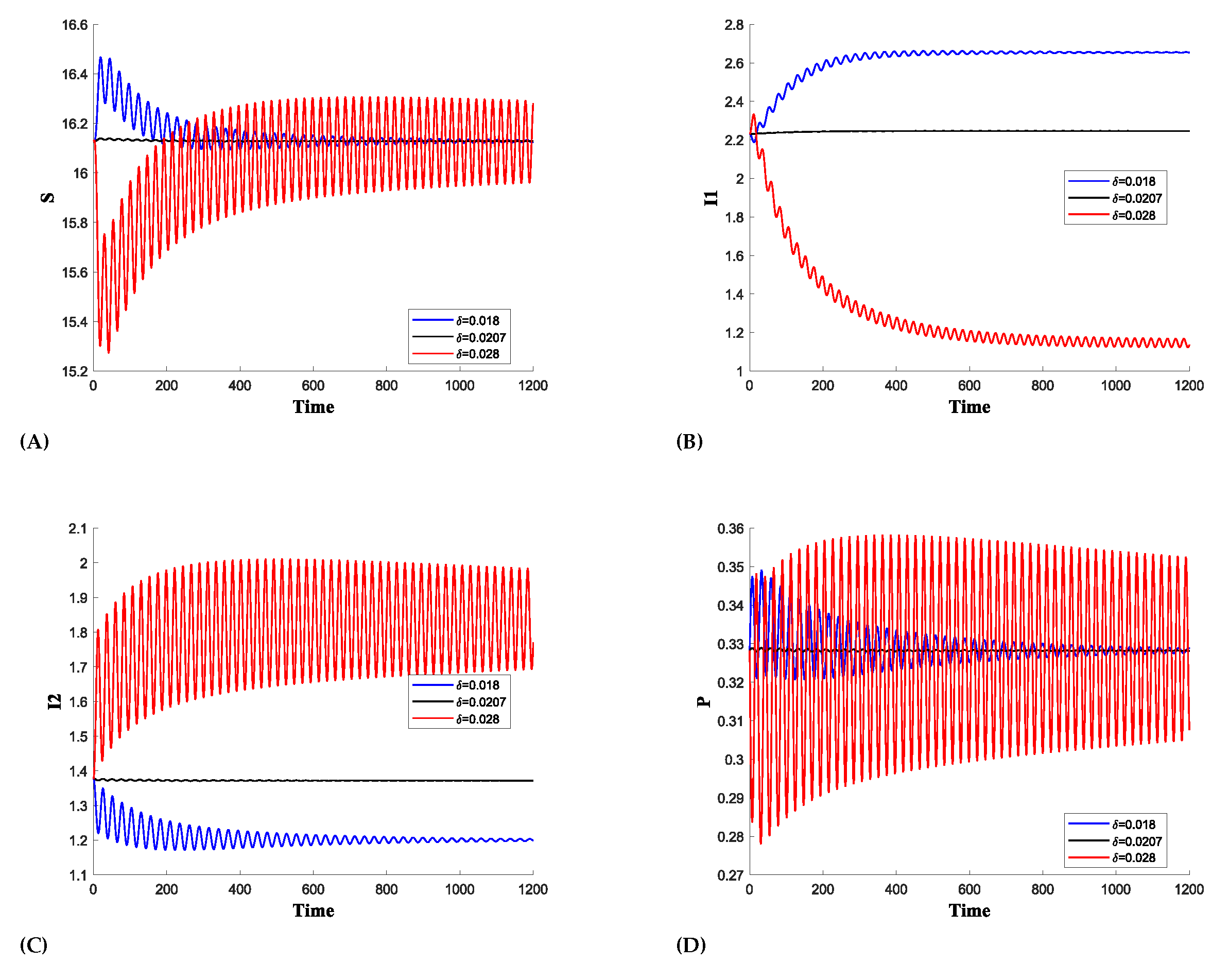
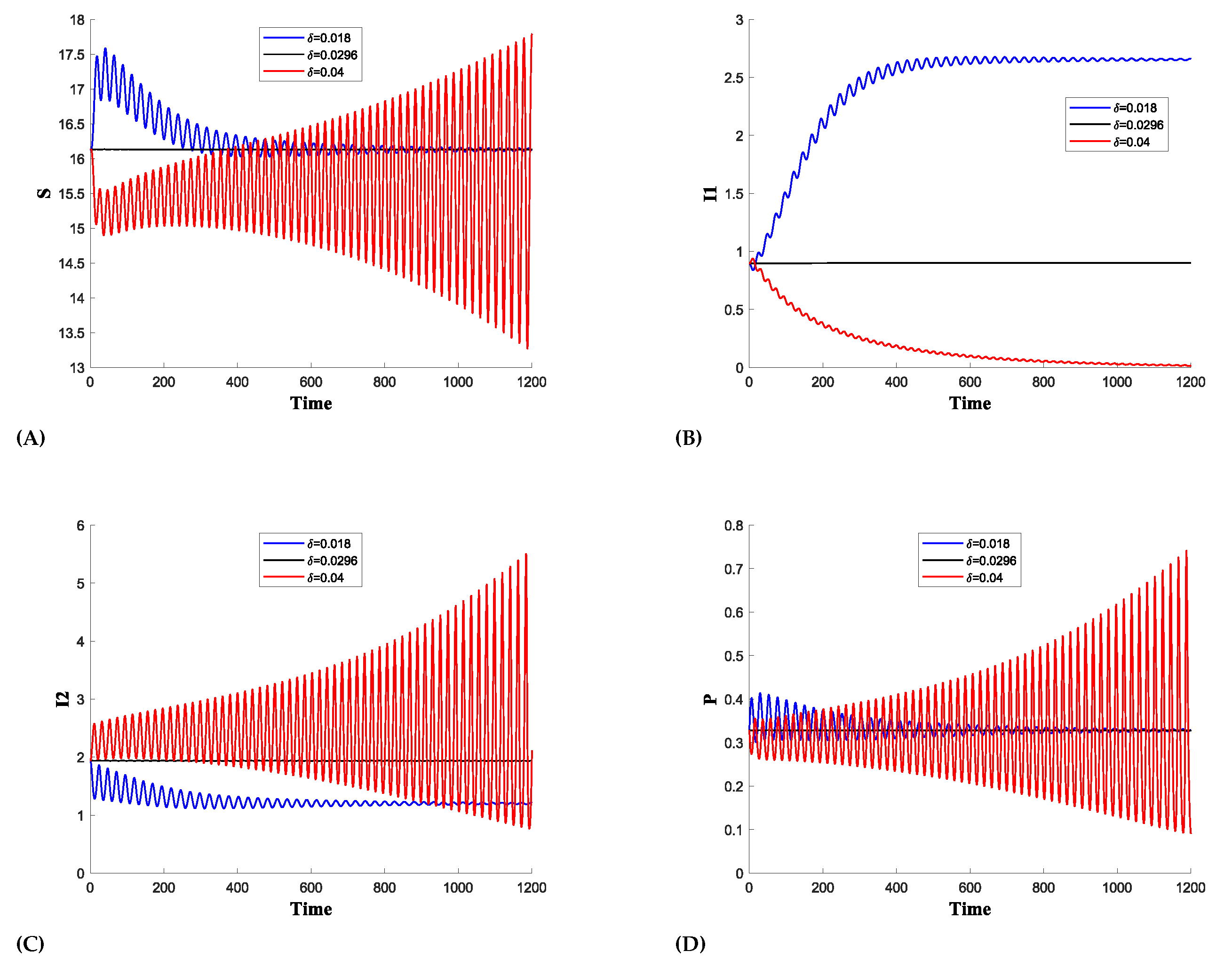
(b)Effect of death of predator due to prey herd( $δ$ ): In Figure 6, the parameter

δ

represents the rate of predator mortality due to the herd effect, and we also observe a Hopf bifurcation on this parameter at

δ = δ^{*} = 0.0296

where the First Lyapunov coefficient(FLC) is

- 1.364586 \times 10^{- 4}

which is negative thus showing Supercritical Hopf bifurcation. At

δ = δ^{* *} = 0.0207

, we have a Hopf point with First Lyapunov Coefficient

2.085063 \times 10^{- 4}

which is positive thus confirming subcritical Hopf bifurcation. For an increased death rate of the predator, the oscillation amplitude of

I_{1}

becomes very low because there are fewer predators to attack each population. As a result, due to the high recovery and death rates,

I_{1}

diminishes to zero.

Figure 4. The time series plot for the Supercritical Hopf bifurcation showing the influence of the prey herd shape (k) on : (A) Susceptible prey,(B) prey infected with strain 1, (C) prey infected with strain 2, (D) Predator population.

Figure 5. Hopf curve for

k - e_{1}

parametric space where GH represents Generalized Hopf point.

Figure 5. Hopf curve for

k - e_{1}

parametric space where GH represents Generalized Hopf point.

We demonstrate that the oscillation amplitude of

I_{1}

is very low for higher values of

δ

, as shown in Figure 6b. Furthermore, a switching mechanism is observed between

I_{1}

and

I_{2}

. In Figure 7, for

δ = 0.018

I_{1}

is higher while

I_{2}

is dying, and for

δ = 0.028

I_{1}

declines while

I_{2}

becomes more prominent. However, oscillations are still present for higher values of

δ

, though with a reduced amplitude due to the limited number of predators attacking each population. Figure 8 shows that only one infection survives, as

I_{1}

dies, while the

I_{2}

shows the growing oscillations for higher value of

δ

Figure 6. The Supercritical Hopf-bifurcation diagram for

δ

shows the onset of periodic oscillations following the bifurcation point at

δ = δ^{*} = 0.0296

. In the diagram, red and blue colors indicate the maximum and minimum values of the positive solution during the steady-state phase, respectively. For values of

δ

less than

δ^{*}

, the convergence of the maximum and minimum values indicates the stability of

E^{*}

. Beyond this point, the solution begins to oscillate between these maximum and minimum values, indicating a loss of stability.

Figure 6. The Supercritical Hopf-bifurcation diagram for

δ

shows the onset of periodic oscillations following the bifurcation point at

δ = δ^{*} = 0.0296

. In the diagram, red and blue colors indicate the maximum and minimum values of the positive solution during the steady-state phase, respectively. For values of

δ

less than

δ^{*}

, the convergence of the maximum and minimum values indicates the stability of

E^{*}

. Beyond this point, the solution begins to oscillate between these maximum and minimum values, indicating a loss of stability.

Figure 7. The time series plot for the Subcritical hopf bifurcation showing the influence of the predator mortality due to prey herd (

δ

) on: (A) Susceptible prey,(B) prey infected with strain 1, (C) prey infected with strain 2, (D) Predator population

Figure 7. The time series plot for the Subcritical hopf bifurcation showing the influence of the predator mortality due to prey herd (

δ

) on: (A) Susceptible prey,(B) prey infected with strain 1, (C) prey infected with strain 2, (D) Predator population

Figure 8. The time series plot for the Supercritical hopf bifurcation showing the influence of the predator mortality due to prey herd (

δ

) on: (A) Susceptible prey,(B) prey infected with strain 1, (C) prey infected with strain 2, (D) Predator population

Figure 8. The time series plot for the Supercritical hopf bifurcation showing the influence of the predator mortality due to prey herd (

δ

) on: (A) Susceptible prey,(B) prey infected with strain 1, (C) prey infected with strain 2, (D) Predator population

8. Conclusions

In this article, we studied the dynamics of two strains of infection in the prey population. The disease transmission is not vertical,i.e. not transferable to offspring. The susceptible prey is assumed to form a herd against predators. In 2D, prey herd for a circle or square is

0.5

, and in 3D, for a sphere, it is

0.67

. We have generalized the rate of prey herd between 0 and 1. Also, we have assumed predator mortality due to prey herd. According to [21], prey on the circumference of the herd can injure predators. The presented model is well-posed and all the solutions are positive and bounded. We identified the biologically feasible equilibrium points and discussed the stability criteria for the interior equilibrium point where all populations coexist. Further, it was observed that the ecosystem cannot disappear since the trivial equilibrium point

E_{1} (0, 0, 0, 0)

is a saddle point i.e. inherently unstable which is a positive point for the given model. We also show the only healthy prey equilibrium point

E_{2} (K, 0, 0, 0)

is locally asymptotically stable under certain conditions and if the basic reproduction number

R_{0} < 1

. If

R_{0}^{1} > 1

then prey infected with the first strain will dominate and if

R_{0}^{2} > 1

then prey infected with the second strain will dominate. Elena et al. [24,25] analyzed two different types of models with two strains of infection in the prey population. Their mathematical findings display no coexistence with both disease strains. Similarly, Roman et al. [26] considered two strain infections in predators, Bosica et al. [27] considered two strain infections in prey with mutualism but could not establish coexistence of equilibrium with both disease strains. However, our work shows the existence of an interior equilibrium point

E^{*} (S^{*}, I_{1}^{*}, I_{2}^{*}, P^{*})

where both the infections coexist. In Figure 3 we detected a supercritical hopf bifurcation about

E^{*}

for prey herd shape

k = 0.722467

. Gupta and Dubey [12] observed a resembling situation for

k = 0.6621

in the case of one infection strain. Moreover, in Figure 2 our research reveals that for a particular herd shape at

k = 0.950245

prey infected with strain 1 dies and other populations settle to a stable limit cycle. Further investigations demonstrate changes in population on increasing the mortality rate(

δ

) of predators due to prey herd. It is observed in Figure 6, that at

δ = 0.0296

system undergoes supercritical Hopf bifurcation and a stable limit cycle bifurcates. In addition to this, it is seen in Figure 8, for high values of

δ

(say

= 0.04

) prey infected with strain 1 dies out. Further, in the model we have detected significant bifurcation phenomena, consisting of the generalized Hopf bifurcation, the cusp point, and the limit point of cycles (LPC) curve. However, a detailed analysis and extensive investigation of these bifurcations, including their biological inferences and further understanding of the system’s dynamics, will be attended in future work. These factors hold significant prospects in understanding the complex interplay between spread of infection and population dynamics and will form the basis of later studies.

Author Contributions

Conceptualization, V.P. and B.D.; methodology, S.J.; software, S.J.; validation, S.J. and V.P.; formal analysis, S.J. and P.M.; investigation, S.J.; resources, P.M. and V.P. and B.D.; data curation, S.J.; writing—original draft preparation, S.J., B.D., Q.Z., V.P. and P.M.; writing—review and editing,S.J., B.D., Q.Z., V.P. and P.M.; visualization, V.P. and B.D.; supervision, V.P. and P.M.; project administration, V.P.; funding acquisition, P.M. and V.P. All authors have read and agreed to the published version of the manuscript.

Funding

This research received no external funding.

Conflicts of Interest

The authors declare no conflicts of interest.

References

Upadhyay, R.K.; Iyengar, S.R. K.; Rai, V. Chaos: an ecological reality? International Journal of Bifurcation and Chaos 1998, 08, 1325–1333. [Google Scholar] [CrossRef]
Aziz-Alaoui, M. Study of a Leslie–Gower-type tritrophic population model. Chaos Solitons & Fractals 2022, 14, 1275–1293. [Google Scholar] [CrossRef]
Verma, H.; Antwi-Fordjour, K.; Hossain, M.; Pal, N.; Parshad, R.D.; Mathur, P. A “Double” fear effect in a tri-trophic food chain model. The European Physical Journal Plus 2021, 136. [Google Scholar] [CrossRef]
Verma, H.; Mathur, P. Analysis of chaotic situation in three species food chain model. Ganita 2019, 69, 57–65. [Google Scholar]
Garai, S.; Hossain, M.; Karmakar, S.; Pal, N. Chaos, periodic structures, and multistability: Complex dynamical behaviors of an eco-epidemiological model in parameter planes. Chaos an Interdisciplinary Journal of Nonlinear Science 2023, 33. [Google Scholar] [CrossRef]
Jana, S.; Kar, T. Modeling and analysis of a prey–predator system with disease in the prey. Chaos Solitons & Fractals 2013, 47, 42–53. [Google Scholar] [CrossRef]
Chattopadhyay, J.; Srinivasu, P.; Bairagi, N. Pelicans at risk in Salton sea — an eco-epidemiological model. Ecological Modelling 2001, 136, 103–112. [Google Scholar] [CrossRef]
Gupta, A.; Dubey, B. Bifurcations and multi-stability in an eco-epidemic model with additional food. The European Physical Journal Plus 2022, 137. [Google Scholar] [CrossRef]
Upadhyay, R. K.; Roy, P. Spread of a disease and its effect on population dynamics in an eco-epidemiological system. Communications in Nonlinear Science and Numerical Simulation 2014, 19, 4170–4184. [Google Scholar] [CrossRef]
Ghosh, M.; Li, X.Z. Mathematical modelling of prey-predator interaction with disease in prey. International Journal of Computing Science and Mathematics 2016, 7, 443. [Google Scholar] [CrossRef]
Chattopadhyay, J.; Arino, O. A predator-prey model with disease in the prey. Nonlinear Analysis 1999, 36, 747–766. [Google Scholar] [CrossRef]
Gupta, A.; Dubey, B. Bifurcation and chaos in a delayed eco-epidemic model induced by prey configuration. Chaos Solitons & Fractals 2022, 165, 112785. [Google Scholar] [CrossRef]
Lazebnik, T.; Bunimovich-Mendrazitsky, S. Generic approach for mathematical model of multi-strain pandemics. PloS One 2022, 17, e0260683. [Google Scholar] [CrossRef]
Alexi, A.; Rosenfeld, A.; Lazebnik, T. Multi-species prey–predator dynamics during a multi-strain pandemic. Chaos an Interdisciplinary Journal of Nonlinear Science 2023, 33. [Google Scholar] [CrossRef] [PubMed]
Pandey, V.; Singh, S. The analysis of global stability boundary and multistability in the nonlinear dynamical system of an advanced heavy water reactor. Nuclear Science and Engineering 2017, 188, 187–197. [Google Scholar] [CrossRef]
Pandey, V.; Singh, S. Bifurcation analysis of the simplified models of boiling water reactor and identification of global stability boundary. Nuclear Engineering and Design 2017, 315, 93–103. [Google Scholar] [CrossRef]
Pandey, V.; Singh, S. Bifurcation analysis of density wave oscillations in natural circulation loop. International Journal of Thermal Sciences 2017, 120, 446–458. [Google Scholar] [CrossRef]
Pandey, V.; Singh, S. Detailed bifurcation analysis with a simplified model for advance heavy water reactor system. Communications in Nonlinear Science and Numerical Simulation 2015, 20, 186–198. [Google Scholar] [CrossRef]
Pandey, V.; Singh, S. Characterization of stability limits of Ledinegg instability and density wave oscillations for two-phase flow in natural circulation loops. Chemical Engineering Science 2017, 168, 204–224. [Google Scholar] [CrossRef]
Pandey, V.; Singh, S. Bifurcations emerging from a double Hopf bifurcation for a BWR. Progress in Nuclear Energy 2019, 117, 103049. [Google Scholar] [CrossRef]
Djilali, S.; Cattani, C.; Guin, L. N. Delayed predator–prey model with prey social behavior. the European Physical Journal Plus 2021, 136. [Google Scholar] [CrossRef]
Ajraldi, V.; Pittavino, M.; Venturino, E. Modeling herd behavior in population systems. Nonlinear Analysis Real World Applications 2011, 12, 2319–2338. [Google Scholar] [CrossRef]
Venturino, E.; Petrovskii, S. Spatiotemporal behavior of a prey–predator system with a group defense for prey. Ecological Complexity 2013, 14, 37–47. [Google Scholar] [CrossRef]
Elena, E.; Grammauro, M.; Venturino, E.; Simos, T. E.; Psihoyios, G.; Tsitouras, C.; Anastassi, Z. Ecoepidemics with Two Strains: Diseased Prey. In Proceedings of the AIP Conference, 14 September 2011. [Google Scholar] [CrossRef]
Elena, E.; Grammauro, M.; Venturino, E. Predator’s alternative food sources do not support ecoepidemics with twostrains-diseased prey. Network Biology 2013, 3, 29–44. [Google Scholar]
Roman, F.; Rossotto, F.; Venturino, E. Ecoepidemics with two strains: diseased predators. WSEAS Transactions on Biology and Biomedicine 2011, 8, 73–85. [Google Scholar]
Bosica, C.; De Rossi, A.; Fatibene, N.L.; Sciarra, M.; Venturino, E. Two-strain ecoepidemic systems: the obligated mutualism case. Applied Mathematics & Information Sciences 2015, 09, 1677–1685. [Google Scholar]
Cavoretto, R.; Collino, S.; Giardino, B.; Venturino, E. A two-strain ecoepidemic competition model. Theoretical Ecology 2014, 8, 37–52. [Google Scholar] [CrossRef]
Banerjee, M.; Kooi, B.; Venturino, E. An Ecoepidemic Model with Prey Herd Behavior and Predator Feeding Saturation Response on Both Healthy and Diseased Prey. Mathematical Modelling of Natural Phenomena 2017, 12, 133–161. [Google Scholar] [CrossRef]
Djilali, S. Impact of prey herd shape on the predator-prey interaction. Chaos Solitons & Fractals 2019, 120, 139–148. [Google Scholar] [CrossRef]
Antwi-Fordjour, K.; Westmoreland, S.P.; Bearden, K.H. Dual fear phenomenon in an eco-epidemiological model with prey aggregation. The European Physical Journal Plus 2024, 139. [Google Scholar] [CrossRef]
Kooi, B.W.; Venturino, E. Ecoepidemic predator–prey model with feeding satiation, prey herd behavior and abandoned infected prey. Mathematical Biosciences 2016, 274, 58–72. [Google Scholar] [CrossRef] [PubMed]
Ruan, S.; Xiao, D.; Beier, J.C. On the Delayed Ross–Macdonald Model for Malaria Transmission. Bulletin of Mathematical Biology 2008, 70, 1098–1114. [Google Scholar] [CrossRef] [PubMed]
Saha, S.; Samanta, G.P. Analysis of a predator–prey model with herd behavior and disease in prey incorporating prey refuge. International Journal of Biomathematics 2019, 12, 1950007. [Google Scholar] [CrossRef]
Venturino, E. The usefulness of mathematics in agriculture, for the environment and in contrasting diseases: insights from a wide range of simple models. Communications in Applied and Industrial Mathematics 2024, 15, 27–49. [Google Scholar] [CrossRef]
Collino, S.; Venturino, E.; Ferreri, L.; Bertolotti, L.; Rosati, S.; Giacobini, M. Models for two strains of the Caprine Arthritis Encephalitis Virus Disease. In Biomat 2015, Mondaini, R.P.,Eds.; 2016, 297–318. [CrossRef]
Fournié, G.; Walker, P.; Porphyre, T.; Métras, R.; Pfeiffer, D. Mathematical Models of infectious diseases in livestock: Concepts and application to the spread of highly pathogenic Avian influenza virus strain type H5N1. In Springer eBooks; 2011; pp. 183–205. [Google Scholar] [CrossRef]
Doeschl-Wilson, A.; Knap, P.; Opriessnig, T.; More, S. Review: Livestock disease resilience: from individual to herd level. Animal 2021, 15, 100286. [Google Scholar] [CrossRef]
Mandal, D.S.; Samanta, S.; Alzahrani, A.K.; Chattopadhyay, J. STUDY OF a PREDATOR–PREY MODEL WITH PEST MANAGEMENT PERSPECTIVE. Journal of Biological Systems 2019, 27, 309–336. [Google Scholar] [CrossRef]
Verma, H.; Mishra, V.N.; Mathur, P. Effectiveness of lock down to curtail the spread of corona virus: A mathematical model. ISA Transactions 2022, 124, 124–134. [Google Scholar] [CrossRef]
Mikheev, V.N.; Pasternak, A.F. Defense behavior of fish against predators and parasites. Journal of Ichthyology 2006, 46, S173–S179. [Google Scholar] [CrossRef]
Demandt, N.; Praetz, M.; Kurvers, R.H.J.M.; Krause, J.; Kurtz, J.; Scharsack, J.P. Parasite infection disrupts escape behaviours in fish shoals. In Proceedings of the Royal Society B Biological Sciences, 4 November 2020. [Google Scholar] [CrossRef]
Allan, B.J.M.; Illing, B.; Fakan, E.P.; Narvaez, P.; Grutter, A.S.; Sikkel, P.C.; McClure, E.C.; Rummer, J.L.; McCormick, M.I. Parasite infection directly impacts escape response and stress levels in fish. Journal of Experimental Biology 2020. [Google Scholar] [CrossRef]
Shi, Y.; Zhao, H.; Zhang, X. Dynamics of a multi-strain malaria model with diffusion in a periodic environment. Journal of Biological Dynamics 2022, 16, 766–815. [Google Scholar] [CrossRef]
Roldan, J.A.M.; Otranto, D. Zoonotic parasites associated with predation by dogs and cats. Parasites & Vectors 2023, 16. [Google Scholar] [CrossRef]
Lamichhane, B.; Mawad, A.M.M.; Saleh, M.; Kelley, W.G.; Harrington, P.J.; Lovestad, C.W.; Amezcua, J.; Sarhan, M.M.; Zowalaty, M.E.E.; Ramadan, H.; Morgan, M.; Helmy, Y.A. Salmonellosis: An overview of epidemiology, pathogenesis, and innovative approaches to mitigate the antimicrobial resistant infections. Antibiotics 2024, 13, 76. [Google Scholar] [CrossRef]
Siddik, S.B.M.; Abdullah, F.A.; Ismail, A.I.M. Mathematical Model of Dengue Virus with Predator-Prey Interactions. Sains Malaysiana 2020, 49, 1191–1200. [Google Scholar] [CrossRef]
De Araújo, R.G.; Jorge, D.C.; Dorn, R.C.; Cruz-Pacheco, G.; Esteva, M.L.M.; Pinho, S.T. Applying a multi-strain dengue model to epidemics data. Mathematical Biosciences 2023, 360, 109013. [Google Scholar] [CrossRef] [PubMed]
Ogunlade, S.T.; Adekunle, A.I.; McBryde, E.S.; Meehan, M.T. Modelling the ecological dynamics of mosquito populations with multiple co-circulating Wolbachia strains. Scientific Reports 2022, 12. [Google Scholar] [CrossRef]
Xue, L.; Zhang, H.; Sun, W.; Scoglio, C. Transmission dynamics of multi-strain dengue virus with cross-immunity. Applied Mathematics and Computation 2021, 392, 125742. [Google Scholar] [CrossRef]
Martcheva, M. Evolutionary consequences of predation for pathogens in prey. Bulletin of Mathematical Biology 2009, 71, 819–844. [Google Scholar] [CrossRef]
Dhooge, A.; Govaerts, W.; Kuznetsov, Y.A. MATCONT. ACM Transactions on Mathematical Software 2003, 29, 141–164. [Google Scholar] [CrossRef]

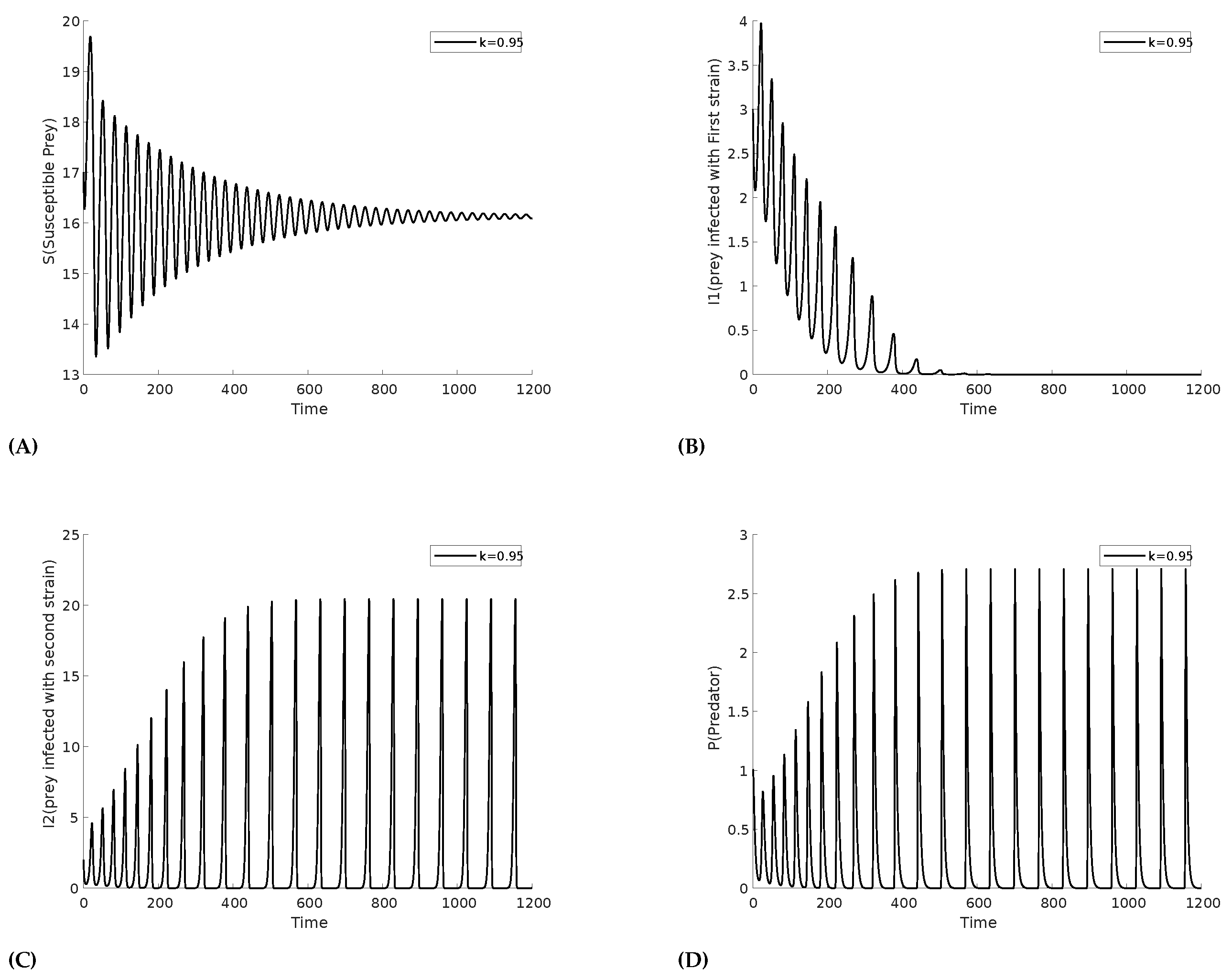
Figure 2. Time series plot depicting the decline of (B) prey infected with strain 1, alongside other variables: (A) Susceptible prey, (C) prey infected with strain 2, (D) Predator population.

Figure 3. The Hopf-bifurcation diagram for k shows the onset of periodic oscillations following the bifurcation point at

k = k^{*} = 0.722

. In the diagram, red and blue colors indicate the maximum and minimum values of the positive solution during the steady-state phase, respectively. For values of k less than

k^{*}

, the convergence of the maximum and minimum values indicates the stability of

E^{*}

. Beyond this point, the solution begins to oscillate between these maximum and minimum values, indicating a loss of stability.

Figure 3. The Hopf-bifurcation diagram for k shows the onset of periodic oscillations following the bifurcation point at

k = k^{*} = 0.722

. In the diagram, red and blue colors indicate the maximum and minimum values of the positive solution during the steady-state phase, respectively. For values of k less than

k^{*}

, the convergence of the maximum and minimum values indicates the stability of

E^{*}

. Beyond this point, the solution begins to oscillate between these maximum and minimum values, indicating a loss of stability.

Disclaimer/Publisher’s Note: The statements, opinions and data contained in all publications are solely those of the individual author(s) and contributor(s) and not of MDPI and/or the editor(s). MDPI and/or the editor(s) disclaim responsibility for any injury to people or property resulting from any ideas, methods, instructions or products referred to in the content.

© 2024 by the authors. Licensee MDPI, Basel, Switzerland. This article is an open access article distributed under the terms and conditions of the Creative Commons Attribution (CC BY) license (http://creativecommons.org/licenses/by/4.0/).

Copyright: This open access article is published under a Creative Commons CC BY 4.0 license, which permit the free download, distribution, and reuse, provided that the author and preprint are cited in any reuse.