Preprint
Article

Short-term Wind Power Forecasting Based on OMNIC and Adaptive Fractional Order Generalized Pareto Motion Model

Altmetrics

Downloads

54

Views

18

Comments

0

Submitted:

12 October 2024

Posted:

15 October 2024

You are already at the latest version

Alerts
Abstract
With the rapid development of renewable energy, accurately forecasting wind power is crucial for the stable operation of power systems and effective energy management. This paper proposes a short-term wind power forecasting method based on the Orthogonalized Maximal Information Coefficient (OMNIC) combined with an Adaptive Fractional Generalized Pareto Motion (fGPm) model. The method quantifies the influence of meteorological factors on wind power prediction and identifies the optimal set and number of influencing factors. The model accounts for long-range dependence (LRD) in time series data and constructs an uncertainty model using the properties and parameters of the fractional generalized Pareto distribution (GPD), significantly improving prediction accuracy under nonlinear conditions. The proposed approach was validated using a real dataset from a wind farm in northwest China and compared with other models such as Convolutional Neural Network-Long Short-Term Memory (CNN-LSTM) and Convolutional Neural Network-Gated Recurrent Unit (CNN-GRU). Results demonstrate that the adaptive fGPm model significantly reduces wind power forecasting errors, offering high accuracy and robustness. This method provides practical value in alleviating peak voltage and frequency regulation challenges in power systems and in promoting the integration of wind power into the grid.
Keywords: 
Subject: Engineering  -   Electrical and Electronic Engineering

1. Introduction

The Wind energy, as one of the most critical renewable energy sources, plays a significant role in the planning and scheduling of power systems. However, the intermittency, high variability, and strong stochastic nature of wind power generation present substantial challenges and adverse impacts on the integration of wind power into the grid [1]. Consequently, accurate wind power forecasting has become one of the key strategies to address the issues related to wind power integration [2].
To tackle this issue, current research primarily focuses on improving feature input and constructing precise models to enhance the accuracy and reliability of wind power forecasting. In terms of feature extraction, researchers utilize feature processing techniques to provide models with richer feature information. For instance, Ju, Y, et al. [3] constructed a novel feature set by analyzing the characteristics of time series raw data from wind farms and neighboring wind farms, proposing the use of Convolutional Neural Networks (CNN) to extract information from input data. Zhao, Y, B, et al. [4] were the first to apply the NeuralProphet model to decompose wind power time series data, accurately capturing the complex nonlinear patterns hidden within wind power time series.
In the realm of model construction, machine learning and deep learning have made remarkable progress as the primary statistical models in the field of wind power forecasting in recent years [5-8]. Liao, S, L, et al. [9]introduced a Light Gradient Boosting Machine (LightGBM) model with strong nonlinear fitting capabilities, which can fully exploit the valuable information in historical wind power operation data. Wang, Y, S, et al.[10]proposed a wind farm output power forecasting model based on the Sliding Time Window (TSW) and Long Short-Term Memory Networks (LSTM) [11,19], effectively fitting the output power curve of the wind farm and achieving accurate wind power prediction. Yu, C, Q, et al. [12] combined Graph Attention Networks (GAT), Gated Recurrent Units (GRU), and Temporal Convolutional Networks (TCN) to effectively extract features from wind power time series data, significantly improving the model's accuracy and robustness. Yang Guohua et al. [13] proposed a short-term wind power forecasting model based on Complementary Ensemble Empirical Mode Decomposition-Sample Entropy (CEEMD-SE), Convolutional Neural Networks (CNN), and Long Short-Term Memory-Gated Recurrent Units (LSTM-GRU)[23], demonstrating that the model effectively enhanced forecasting accuracy, reducing the error by 15.06%. However, deep learning models require the setting of numerous parameters, and hyperparameters determined by expert experience often differ from the optimal parameters needed by the model. Moreover, as the volume of data increases, especially when the model becomes overly complex, more computational resources and training time are required.
To address the aforementioned issues, this paper employs the Orthogonal Maximum Information Coefficient to analyze the correlation between meteorological features and wind power for feature extraction [14], meeting the timeliness requirements of wind power forecasting tasks. Considering the long-range dependence characteristics of wind power [15,16]. an Adaptive Fractional-order Generalized Pareto Motion (fGPm) forecasting model is proposed to cope with the randomness and volatility of wind energy.The main contributions of this paper are as follows:
Since the correlation between variables in industrial data is often nonlinear, using the Orthogonal Maximum Information Coefficient to analyze the correlation between meteorological features and wind power allows for more accurate capture of the nonlinear relationships between variables, thereby improving feature input and meeting the timeliness needs of wind power forecasting tasks.
Research on random sequences with long-range dependence (LRD) characteristics in the field of wind power forecasting remains relatively limited [17,18]. Therefore, the Adaptive Fractional-order Generalized Pareto Motion (fGPm) model is introduced, which considers long-term dependency uncertainty, fully accounts for the influence of past and current states on future states, and more effectively forecasts a series of non-smooth stochastic processes[ 19]. As the environment changes, the rate of variation in the degradation process also changes accordingly. The proposed adaptive diffusion coefficient fGPm demonstrates superiority and robustness in handling data with high jumpiness.
To verify the practicality and effectiveness of the proposed method, a case analysis of wind power data from a wind farm in Northwest China is conducted [20]. Two scenarios are selected for the experiment: one with significant meteorological feature fluctuations in winter from December 12, 2019, 7:00 to December 14, 2019, 19:00 (Case 1), and another with smaller fluctuations in summer from July 12, 2019, 7:00 to July 14, 2019, 19:00 (Case 2), serving as historical feature data[21,22]. These data are used to predict the optimal power change trends of wind power within the next 12, 24, 36, and 48 steps. Compared with previous methods, the model shows higher precision in power forecasting.
The structure of this paper is arranged as follows: Section 2 analyzes the input feature variables that affect wind power, introducing the principles and steps of the Orthogonalized Maximal Information Coefficient (OMNIC) method in data preprocessing[24]. Section 3 discusses the characteristics of the fractional generalized Pareto distribution (GPD)[25] and the physical significance of its parameters, focusing on the analysis of the distribution's long-range dependence (LRD) and heavy-tailed characteristics[26]. Additionally, the mathematical expression of the adaptive fractional generalized Pareto motion (fGPm) model and its incremental form are introduced, exploring the LRD characteristics of fGPm and the process of generating numerical sequences. Section 4 proposes an adaptive fGPm iterative differential forecasting model based on Langevin-type stochastic differential equations (SDE)[27,28], describing its parameter estimation methods. Section 5 conducts experimental validation using measured wind power data from a wind farm in Northwest China, demonstrating the efficiency and applicability of the model through comparisons with other models. Finally, Section 6 summarizes the main research findings of this paper and discusses future research directions.
Innovation: In the field of wind energy, time series forecasting is essential for efficient wind energy resource management, improving the grid's acceptance capacity, and enhancing public safety and quality of life. However, due to wind speed fluctuations, wind power generation always has uncertainty and complexity, necessitating the capture of long-range correlations and predictive models. Existing methods often struggle to address both challenges simultaneously[29,30]. This paper delves into these issues, employing the Orthogonal Maximum Information Coefficient (OMI-Coherence) for feature extraction to improve the accuracy of correlation analysis, and proposes a novel Adaptive fGPm model that can autonomously learn different inter-sequence associations at each time scale. Moreover, by parameterizing the uncertainty inherent in the system during the iteration process, better system performance and convergence are achieved. Experiments applied to multiple real datasets from a wind farm have proven the robustness, accuracy, and effectiveness of the model.

2. Feature Extraction

Within wind farms, a multitude of factors can influence the power output of wind energy, with meteorological characteristics being the most critical, such as wind speed, direction, temperature, humidity, and air pressure[31,32]. Selecting features based solely on the correlation between two variables may lead to significant redundancy among them [33,34]. In this study, we employ the Orthogonalized Maximal Information Coefficient (OMI-Coherence) to analyze the correlation between meteorological characteristics and wind power, which more accurately captures the nonlinear relationships between variables[35]. The specific implementation steps are as follows:
Step 1: Define Mutual Information
For a two-dimensional dataset D = ( X , Y ) composed of variables X and Y, divide the space along each axis into intervals X 0 and Y 0 , forming a grid G of size X 0 × Y 0 [36]. Based on the distribution of D / G , the mutual information between X and Y is defined as:
I ( X , Y ) = i Y 0 j X 0 p ( i , j ) log 2 ( p ( i , j ) p ( i ) p ( j ) )
where p ( i , j ) is the joint probability distribution of X and Y, and p ( i ) and p ( j ) are the marginal probability distributions of X and Y, respectively [37].
Step 2: Calculate and Normalize Mutual Information
From the grid G ,identify the maximum value of mutual information I ( D , X 0 , Y 0 ) as the output. Construct a normalized feature matrix M based on this value[38]. The normalized mutual information matrix M I C for a total sample size of n is given by:
M I C = max X 0 Y 0 < B ( n ) ( M ( X 0 , Y 0 ) ) M ( X 0 , Y 0 ) = I ( D , X 0 , Y 0 ) log 2 min ( X 0 , Y 0 )
Step 3: Compute OMI-Coherence
For the set of variables S = { x 1 , x 2 , x 3 , , x n } and the target variable Y ,calculate the maximal information coefficient value between the feature information of x k + 1 , which is independent of the selected variable set S k , and the target variable Y [39]. This is expressed as:
O MICS ( x k + 1 , S k ) = OMI - Coherence   ( x k + 1 ; Y S k ) = max functions   f , g I ( f ( x i ) ; g ( Y ) ) max ( H ( f ( x i ) ) , H ( g ( Y ) ) )
Here, I ( f ( x i ) ; g ( Y ) ) represents the mutual information between the transformed variables[40].
Step 4: Variable Selection and Ranking
Based on the OMI-Coherence values, select the variable with the highest OMI-Coherence value, then incrementally add other variables according to the ranking rules established [41]. The feature vector selected after the k -th choice is used to construct the final feature sequence:
Preprints 121043 i001
This approach effectively selects the most relevant features from meteorological characteristics for wind power forecasting, reduces redundancy among features, and enhances the performance of the predictive model.

3. Model Principle

3.1. Properties and Parameter Meaning of the Fractional-Order Generalized Pareto Distribution (GPD)

The Generalized Pareto Distribution (GPD) [42]serves as an extension of the Pareto distribution, characterized for modeling the tail behavior of probability distributions with heavier tails. Its Probability Density Function (pdf) is:
f ( x | μ , δ , α ) = 1 2 δ [ 1 + 1 α δ | x μ | ] 1 α
In this context, μ represents the location parameter of the distribution, δ denotes the scale parameter, and α signifies the shape parameter[43].
Figure 1 illustrates the Generalized Pareto Distribution (GPD) with its tail decaying in accordance with a power law. The larger the value of the shape parameter α ( 0 , 2 ] , the more pronounced the heavy-tailed nature of the distribution, resulting in a more rapid decrease within the same time frame[44]. Conversely, a smaller α indicates a greater impulsiveness in the sequence, where anomalies occurring further from the central position have a more substantial impact [45].
As shown in Figure 2, the scale parameter δ of the GPD signifies the extent of deviation from the mean. When δ 0 it reflects the dispersion of the distribution around the mean, and in a particular case, it is analogous to the variance of a normal distribution [46].
Hence, if a stochastic process X ( i ) exhibits power-law decay in its probability distribution, characterizing heavy tails, it will also manifest long-range dependence (LRD) characteristics in the realm of its autocorrelation function [47]
3.2. fractional-Order Generalized Pareto Motion (FGPM) Model and Long-Range Dependence (LRD) Characteristics
In the literature, a class of Fractional-order Generalized Pareto Motion (fGPm) models, founded on stochastic Weyl integrals [48], is defined with the following expression:
B H ( t ) = { a [ ( t s ) + H 1 2 ( s ) + H 1 2 ] + b [ ( t s ) H 1 2 ( s ) H 1 2 ] } B ( d s )
In which ( x ) + H 1 2 = ( x ) H 1 2 = { x , x > 0 0 , x 0 , a , b are real constants, and satisfy | a | + | b | > 0 .The Hurst index determines the correlation between the past at time t and the future at time s . Its autocorrelation function is given by:
R B H ( t , s ) = Γ ( 1 2 H ) cos π H π H ( H + 1 / 2 ) Γ ( H + 1 / 2 ) [ | t | 2 H + | s | 2 H | t s | 2 H ]
The autocorrelation function of the fGPm varies over time, as the characteristics of wind power generation and the impact of multi-dimensional environmental factors on wind power output exhibit non-stationarity in industrially collected data. Consequently, the long-range dependence (LRD) characteristics of the fGPm model are determined by the relationship between the self-similarity parameter H and α . The larger the product of H and α , the stronger the LRD characteristics of the fGPm model, leading to a more complex and variable trend in the stochastic sequence. When 0 < H < 0 . 5 , B H ( t ) possesses anti-persistence, indicating that the past correlations of the fGPm model are inversely related to future trends. Conversely, when f α , H ( a , b ; t , s ) ,the integral kernel function f α , H ( a , b ; t , s ) changes very slowly with the variable s [49], causing the integral of the kernel function to diverge at infinity. This persistent effect endows the fGPm model with LRD characteristics, making it a suitable model for forecasting.

3.3. Generation of Numerical Sequences for fractional-Order Generalized Pareto Motion (fGPM) Processes

The central idea of long-range dependent (LRD) stochastic model forecasting is to generate numerical sequences using stochastic models to approximate the actual wind power random sequences. Compared to other methods, there is an improvement in the length and accuracy of the forecast. The expression of the fGPm model is presented in Equation (8) as follows:
P H , α ( t ) = { a [ ( t s ) + H 1 α ( s ) + H 1 α ] + b [ ( t s ) H 1 α ( s ) H 1 α ] } p ( d s )
The fGPm is defined using the Riemann-Liouville fractional integral [50] as follows:
P H , a ( t ) = 1 Γ ( H + 1 2 ) 0 t ( t τ ) H 1 2 p ( d τ )
In which Γ ( x ) = 0 t x 1 e t d t denotes the gamma function, and H represents the calculated Hurst value. By discretizing the increment P H , α ( t ) of the fGPm model, the model generates a stationary increment sequence, that is, the fractional-order Lévy stable noise sequence X H , α ( t ) [51], which is expressed as (Equation 10):
X H , α ( t ) = P H , α ( t + 1 ) P H , α ( t ) = { a [ ( t + 1 s ) + H 1 / α ( s ) + H 1 / α ] + b [ ( t + 1 s ) H 1 / α ( s ) H 1 / α ] } p d s
Fractional Lévy stable white noise w α ( s ) is passed through a fractional-order filter to generate fractional Lévy stable noise. Subsequently, integrating or accumulating this noise yields the numerical simulation sequence of the fGPm model, with the expression provided as follows:
P H , α = 1 Γ ( α + 1 ) { a [ ( t + 1 s ) + H 1 / α ( s ) + H 1 / α ] + b [ ( t + 1 s ) H 1 / α ( s ) H 1 / α ] } ω a ( s ) d s
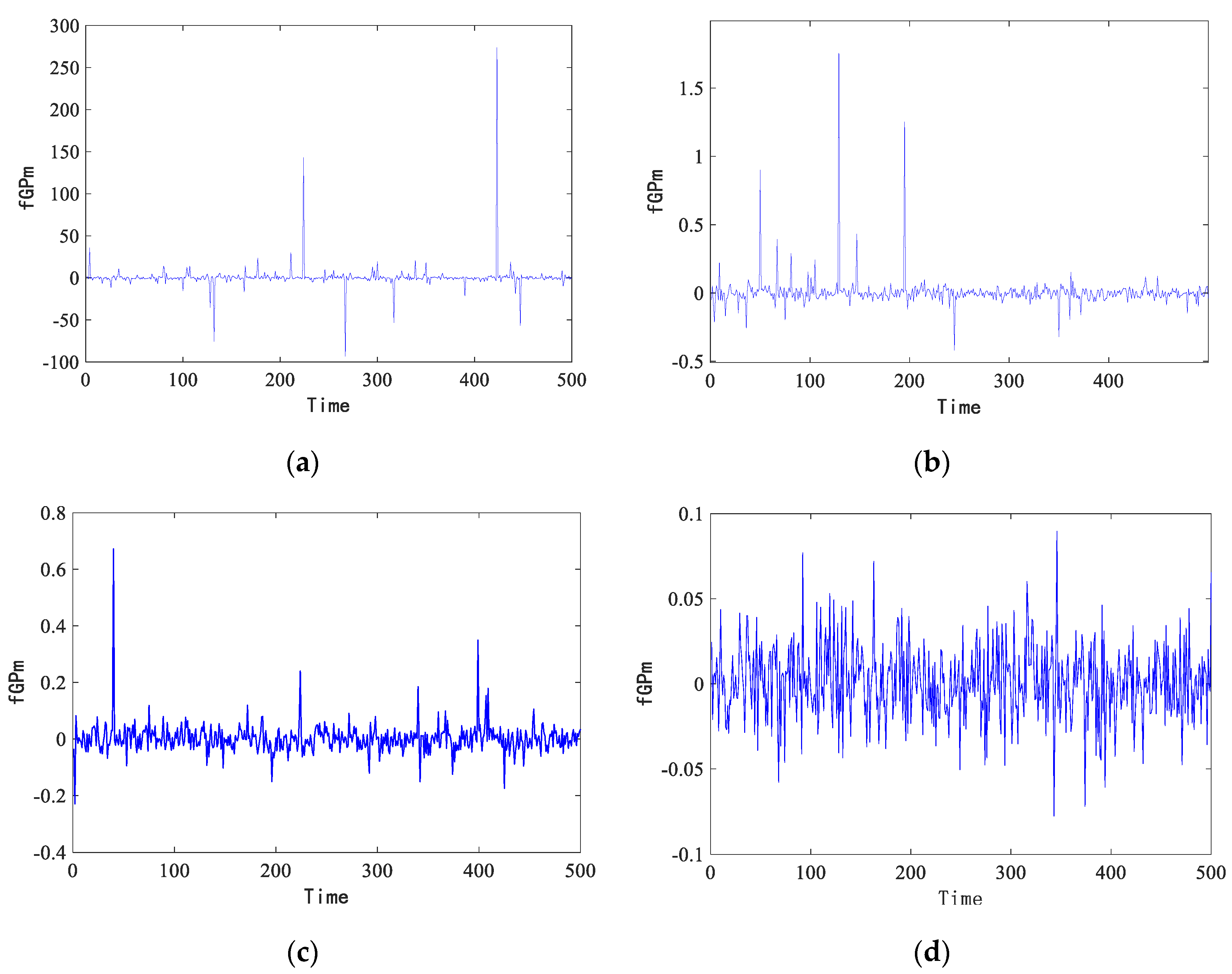
As illustrated in Figure 3, when 0 . 5 H 1 , it is observable that as the value of α increases, the stochastic fluctuations of the fGPm model become less pronounced and occur more rapidly. This implies a diminishing impulsiveness characterized by heavy tails and sharp peaks,
with the long-range dependence (LRD) properties becoming increasingly evident.

3.4. Establishing an Uncertainty Model with Adaptive fGPm

Uncertainty is a pivotal element in wind power forecasting, predominantly stemming from environmental noises that encompass the random variations of meteorological attributes such as wind speed, direction, and temperature. To capture these uncertainties more precisely, this paper proposes an Adaptive Fractional-order Generalized Pareto Motion (fGPm) model featuring a self-adjusting diffusion coefficient. This model is adept at updating the evolution within stochastic processes in a self-adaptive manner, offering a more robust modeling of trend uncertainties for the prediction of wind power.
The definition of the adaptive diffusion coefficient is presented in Equation 12:
σ H ( t ) = σ H ( t 1 ) + ε
In Equation 12, the stochastic sequence ε ~ N ( 0 , σ ε 2 ) reflects the variations in environmental noise, while σ ε 2 measures the intensity of randomness. The diffusion coefficient is initialized at 1 and, over time and with the accumulation of data, it will adaptively adjust according to actual observed values.
The general form of the driving process for the Adaptive Fractional-order Generalized Pareto Motion (fGPm) model, as presented in [52] (Equation 13), is expressed as follows:
X ( t ) = 1 2 X H , α ( t ) + σ H ( t ) P H , α

4. Forecast Model Construction

4.1. Establishment of Iterative Differential Forecasting Model

A. A. Stanislavsky et al. [31] introduced a FARIMA model incorporating Pareto noise, which serves as a discrete-time analogue of the fractional Langevin equation, accounting for non-Gaussian statistical measures and long-range dependence (LRD) [53]. Building upon this foundation, this paper further explores the Langevin-type stochastic differential equation driven by the Generalized Pareto Motion (GPD) as follows (Equation 14):
d X ( t ) = b ( t , X ( t ) ) d t + δ ( t , X ( t ) ) d p a ( t )
Here, d p a ( t ) represents the increment of the Generalized Pareto Motion; replacing P H , a ( t ) with P a ( t ) yields the Langevin-type stochastic differential equation driven by the fGPm as follows (Equation 15):
d X H , a ( t ) = μ ( t , X H , a ( t ) ) d t + δ ( t , X H , a ( t ) ) d P H , a ( t )
In this equation, μ is the expected location parameter, and δ is the volatility parameter. Within the adaptive fGPm framework, the iterative forecasting model is constructed based on incremental modeling. By integrating the discrete form of the fractionalorder Ito process with a differential equation, we derive the iterative differential forecasting model based on the adaptive fGPm model (Equation 16):
P H , α ( t + 1 ) = P H , α ( t ) + μ P H , a ( t ) Δ t + δ P H , a ( t ) w α ( t ) ( Δ t ) H 1 2 + 1 α

4.2. Parameter Estimation of the New Feature Function

The precise estimation of the shape parameter α , the location parameter μ , and the diffusion parameter δ is essential for the construction of the predictive model based on the adaptive fGPm. The Log-Likelihood Estimation (MLE) method is utilized to estimate the specific parameters within the adaptive fGPm model framework[54]. The specific process is as follows:
Step 1: First, define the sample sequence | x i | i = 1 N as the sampling data of the adaptive fGPm, where x ( 1 ) x ( 2 ) x ( N ) and so on, in ascending order of the statistical data.
Step 2: Calculate the mean of the sequence μ using Equation (17).
μ = 1 N i = 1 N x i
Step 3: Assume that the random variable, from which all sample sequences x i | i = 1 N are individually drawn, has a probability density function that is a complex function related to. The log-likelihood function for parameters α and δ is then given by Equation (20).
L * ( θ ) = log 2 N i = 1 N log ( 1 θ x i ) N log [ 1 N θ i = 1 N log ( 1 θ x i ) ]
Step 4: When θ < 1 / x ( N ) , the local maximum value θ ^ is computed using the method of maximum likelihood estimation, yielding the following maximum likelihood estimates:
θ ^ = arg max μ L ( θ x i )
The maximum likelihood estimate for α is:
a ^ = N i = 1 N log ( 1 θ ^ x i )
The maximum likelihood estimate for δ is:
δ ^ = 2 a ^ θ ^

5. Experimental Cases and Analysis

5.1. Data Description

To validate the effectiveness of the adaptive fractional-order Generalized Pareto Motion model (fGPm) proposed in this paper for short-term wind power forecasting, a wind power dataset from a wind farm in Northwest China was selected for analysis. The data spans from October 1, 2019, 00:00 to December 25, 2019, 23:45, with a sampling frequency of 30 times per minute. The dataset includes meteorological characteristics and corresponding power data, comprising local temperature, air humidity, atmospheric pressure, wind speed, and direction. By employing Orthogonalized Maximal Information Coefficient (OMI-Coherence) analysis, numerical weather prediction (NWP) data strongly correlated with wind power output were selected as model inputs. The forecasting target is set for wind power within the next 6 to 24 hours, predicted on an hourly average basis. The forecasting model integrates the NWP data from the previous four days, historical power data, and one-day-ahead NWP forecasts to predict the trend of wind power within the next 24 hours.

5.2. Experimental Process

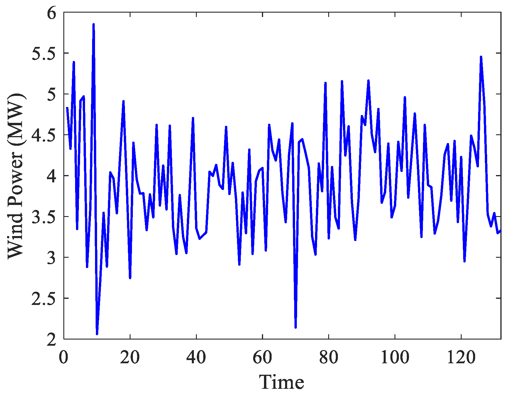
Due to the variability of wind speed, there is an inherent uncertainty in wind power generation. This experiment selects two seasons with different meteorological characteristics for study: one with high fluctuation in winter and another with relatively stable conditions in summer. Specifically, Case One involves data from December 1, 2019, 7:00 to December 11, 2019, 18:00, as shown in Figure 4, totaling 132 data points as the subject of study.
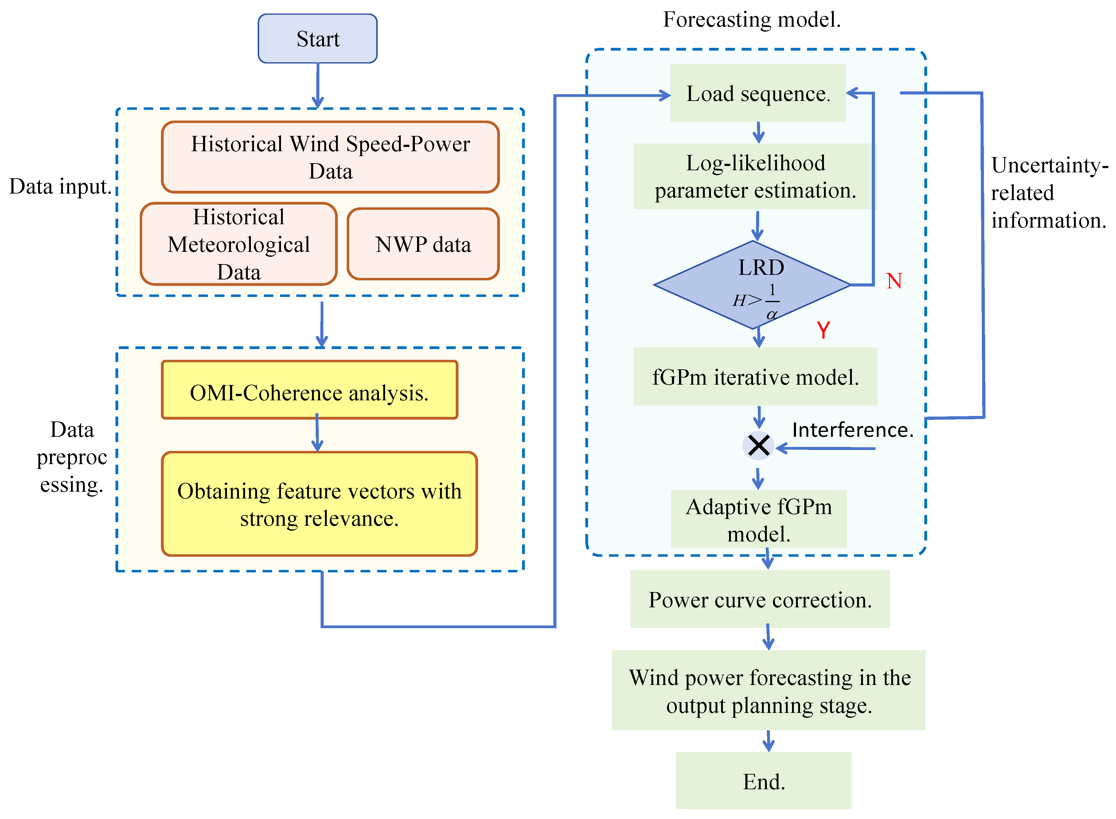
Before using the adaptive fGPm iterative model for prediction, it is first confirmed whether the selected wind power sequence possesses Long-Range Dependence (LRD), ensuring the systematic and scientific nature of the research. The overall experimental procedure is depicted in Figure 5.
As shown in Figure 5, a detailed preprocessing of the historical operation data from the wind farm was first carried out, including the removal of outliers and effective imputation of missing values. Given the coupling between features in the original dataset, before feature extraction and reconstruction, this study applied the Orthogonalized Maximal Information Coherence (OMI-Coherence) method to accurately capture the correlations between meteorological features and power generation. The results indicate that wind speed, wind direction, humidity, temperature, atmospheric pressure, and air density have correlation coefficients with power generation of 0.6808, 0.6267, 0.6426, 0.4645, 0.2763, and 0.1939, respectively.To efficiently extract pivotal features and reduce the model's input dimensionality, this study selected wind direction and speed, which have a strong association with power output, as the input features for the Numerical Weather Prediction (NWP) model, thereby constructing a data sequence with significant predictive value.Subsequently, the study employed an improved maximum likelihood estimation method to precisely estimate the parameters of the wind farm forecasting model, with detailed estimation results presented in Table 1. Based on the condition H < 1 / α , the Hurst indices for the two data ensembles were determined to be 0.8315 and 0.7915, both exceeding the threshold of 0.5, thereby satisfying the criteria for long-range dependence (LRD). To address the uncertainties inherent in wind power forecasting, a diffusion coefficient parameter was introduced to simulate disturbances and enable adaptive adjustments according to actual observed values. This approach not only substantiates the scientific validity of utilizing the adaptive fGPm forecasting model for model construction but also provides a solid foundation for the parameter settings of the wind power trend forecasting model.

5.3. Prediction Results

5.3.1. Case 1: Winter

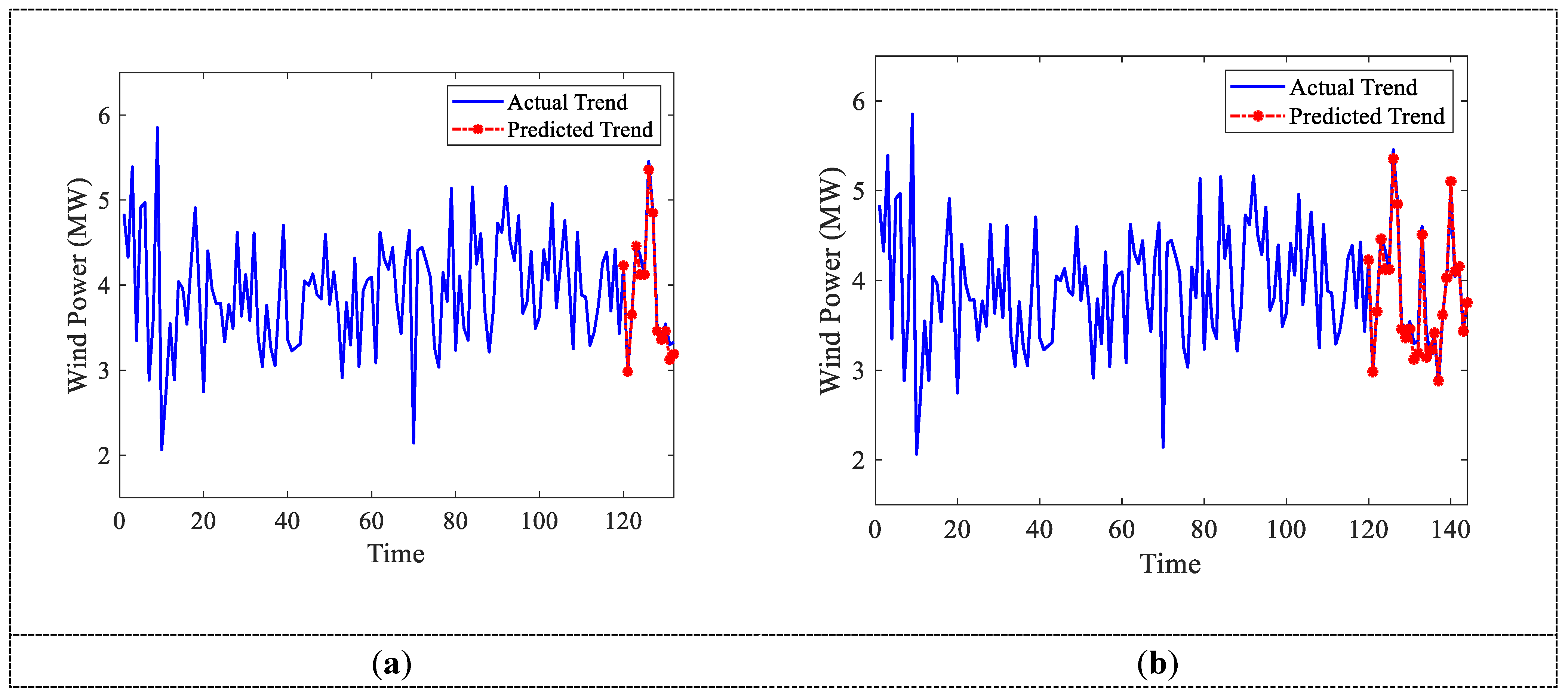
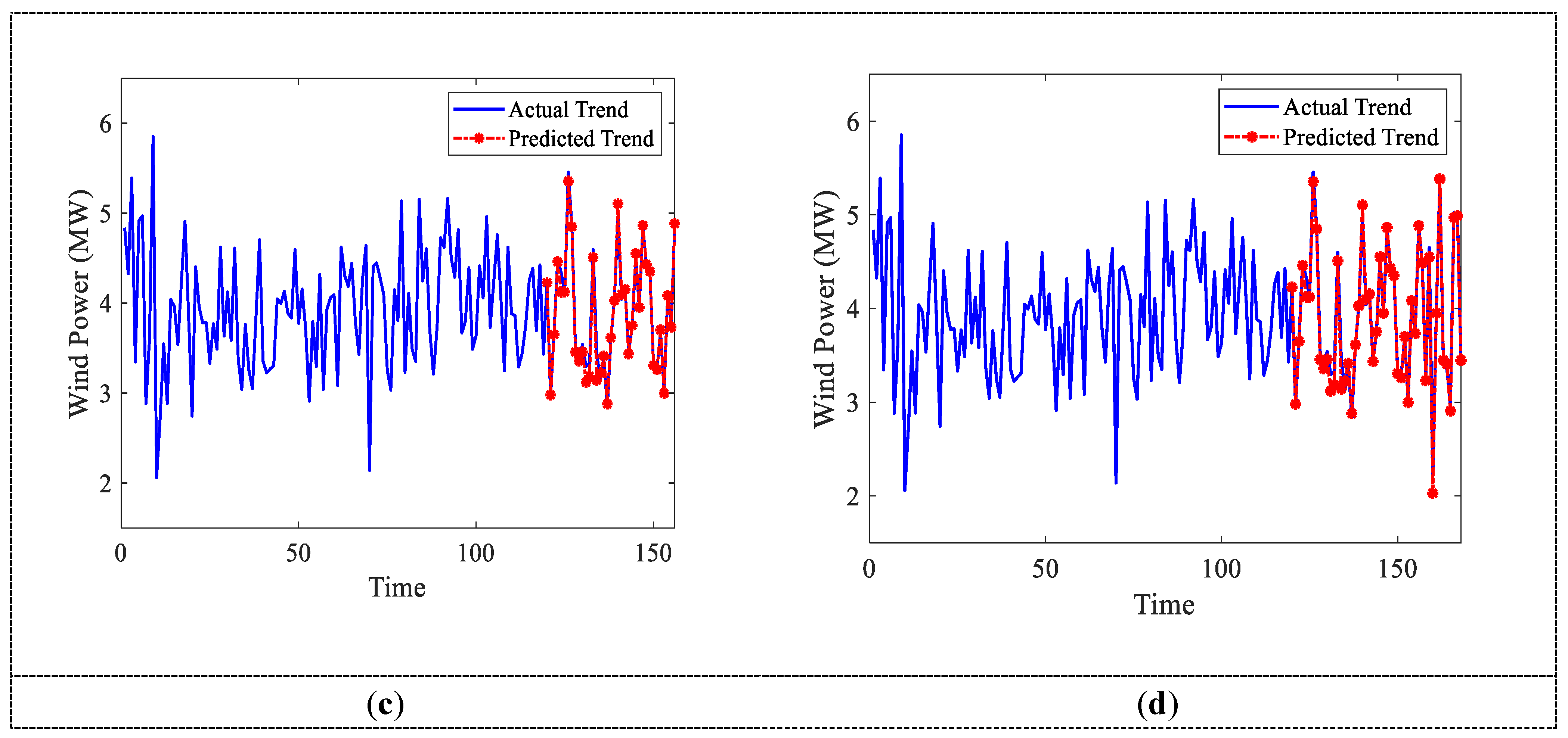
Utilizing the NWP feature values and power data extracted from December 1, 2019, at 07:00 to December 11, 2019, at 18:00 during the winter season as the input sequence, the NWP data for the forthcoming day is employed as historical data to forecast the 12th, 24th, 36th, and 48th wind power values for the subsequent day. Figure 6 illustrates the wind power forecast curve, derived from the adaptive fGPm-based iterative differential prediction model, juxtaposing the predicted and actual wind power values.

5.3.2. Case 2: Summer

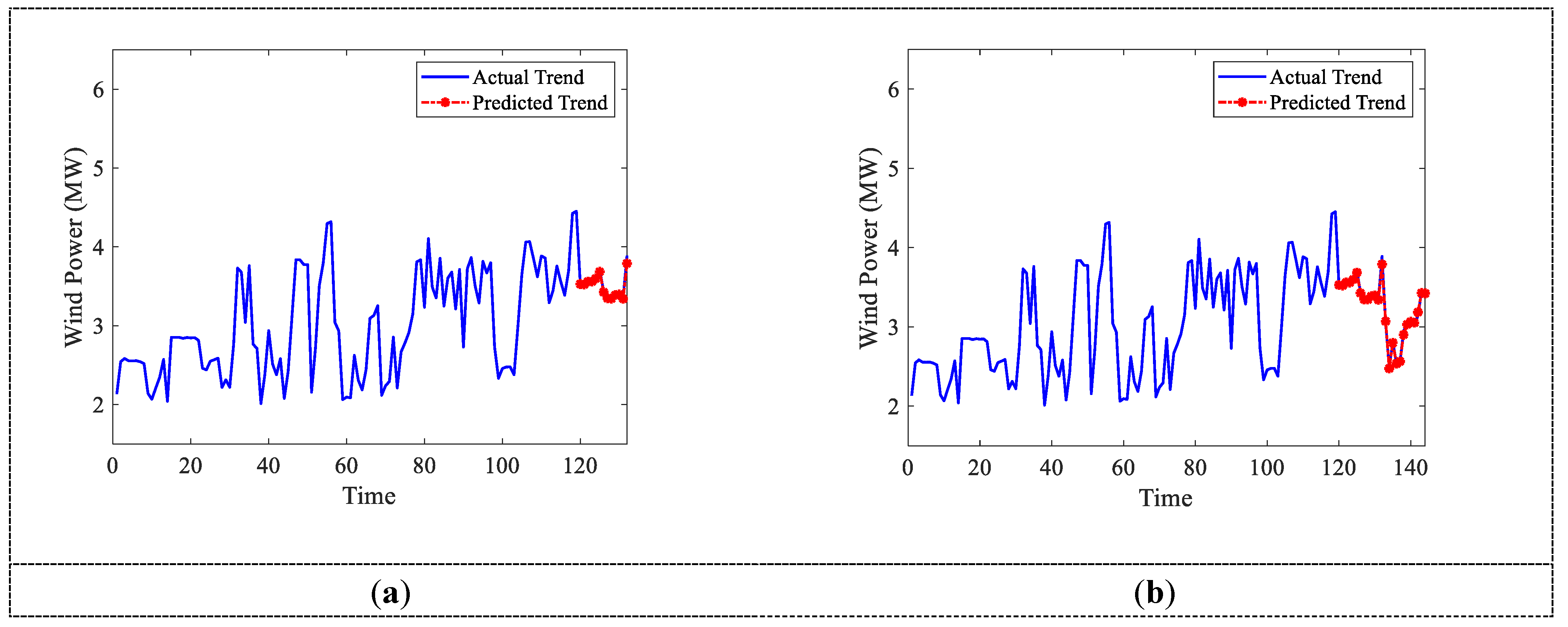
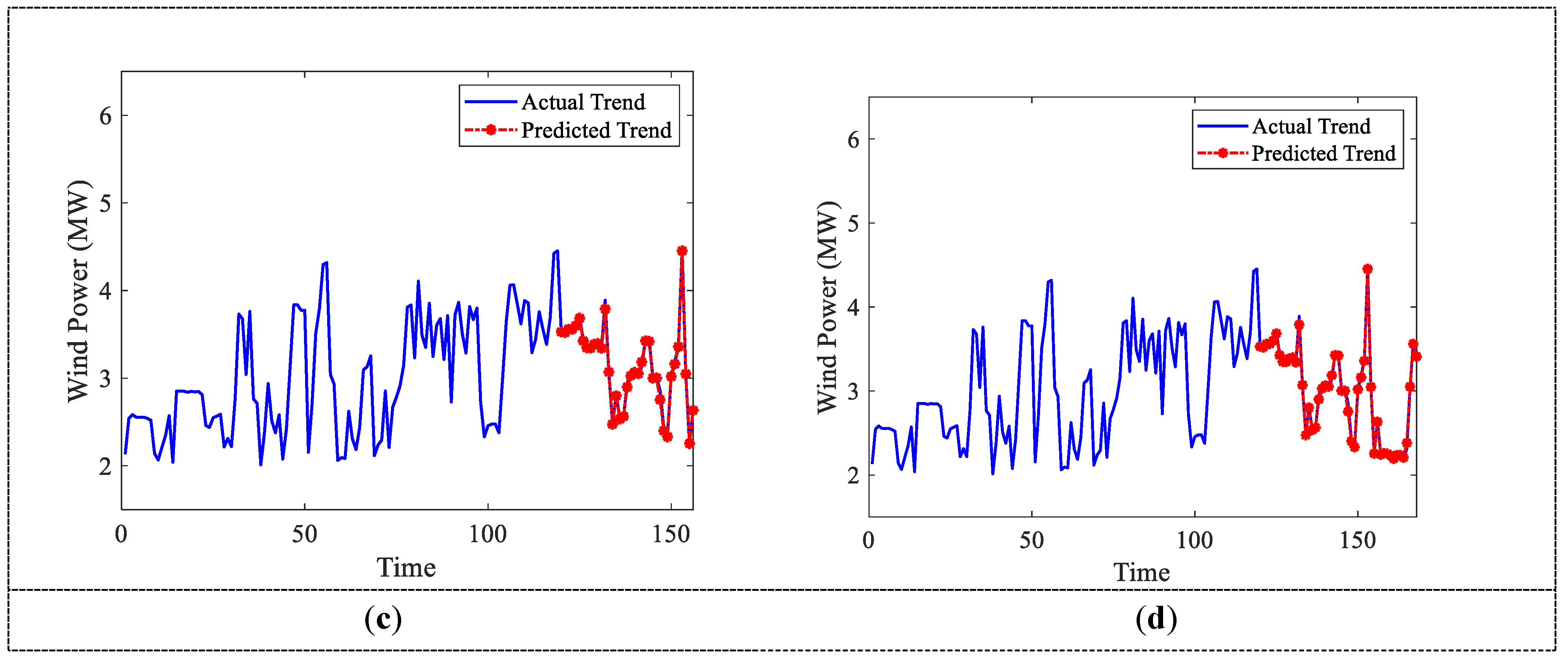
The NWP data and power data from July 1, 2019, 7:00 AM to July 12, 2019, 6:00 PM, along with the NWP data for the following day, were used as historical data. The adaptive fGPm-based iterative differential forecasting model was then applied to predict 12, 24, 36, and 48 wind power values for the next day, as shown in Figure 7.
Figure 6 and Figure 7 distinctly demonstrate the precision of the adaptive Fractional-order Generalized Pareto Motion (fGPm) iterative differential forecasting model in capturing the short-term trends in wind power output for wind turbines. Comparative analysis of the model's forecasts against actual wind power data reveals improved accuracy. Nonetheless, it is observed that the accuracy of wind power trend predictions for the same sequence of samples decreases as the forecasted period extends.
5.4.Model Performance Analysis
To comprehensively evaluate the forecasting accuracy of the adaptive fGPm-based iterative differential prediction model, this paper selects the Root Mean Square Error (RMSE), Mean Absolute Percentage Error (MAPE), and the Coefficient of Determination (R-squared, R2) as metrics for assessing the precision of the final point forecasts. The calculation formulas are as follows:
RMSE = 1 N i = 1 N ( y i y ^ i y cap ) 2
MAPE = 100 % N i = 1 N | y ^ i y i y i |
R 2 = i = 1 N [ ( y i y i ¯ ) ( y ^ i y ¯ i ) ] i = 1 N ( y i y i ¯ ) 2 i = 1 N ( y ^ i y ^ i ¯ ) 2
In Equations (22), (23), and (24), y i and y ^ i represent the actual and forecasted power at time instance i , respectively; y i ¯ and y ^ i ¯ denote the mean values of the actual and forecasted powers, respectively; N is the number of samples; and y cap signifies the installed capacity.
Error Analysis from Table 2 Leads to the Following Conclusions:
RMSE and MAPE:The data in the table reveal that, overall, the RMSE and MAPE values for winter are significantly higher than those for summer, indicating higher forecasting accuracy during the relatively stable wind speeds of summer. Concurrently, within the same season, as the forecast length increases, the RMSE and MAPE values gradually increase, yet maintain relatively small means. This suggests that, although winter forecasting errors may exhibit larger fluctuations in some cases, the general level remains acceptably low.
(1)
Coefficient of Determination( R 2 ):Utilizing the coefficient of determination to assess the final forecast results, the values for summer are notably higher than those for winter. This indicates a greater fit, with the independent variables explaining the dependent variable to a higher degree, thereby signifying a more valuable reference for the forecasting model.
(2)
In summary, the adaptive fGPm iterative differential model has demonstrated a certain level of effectiveness in wind power trend forecasting. In practical applications, when selecting the forecast length, it is necessary to make flexible trade-offs based on specific requirements to achieve an optimal balance.

5.5.Comparison of Different Models

5.5.1. Comparative Analysis of Model Prediction Result

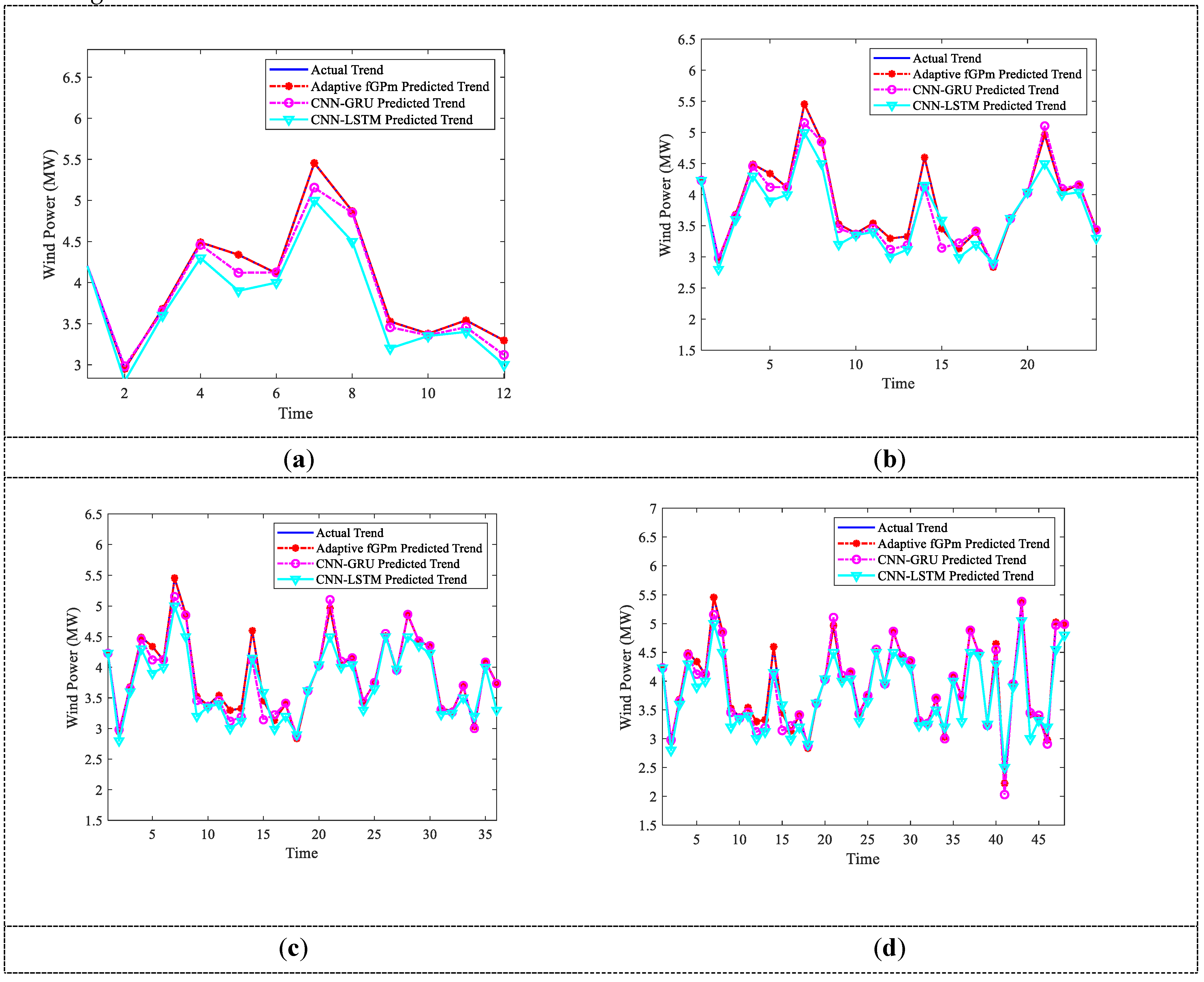
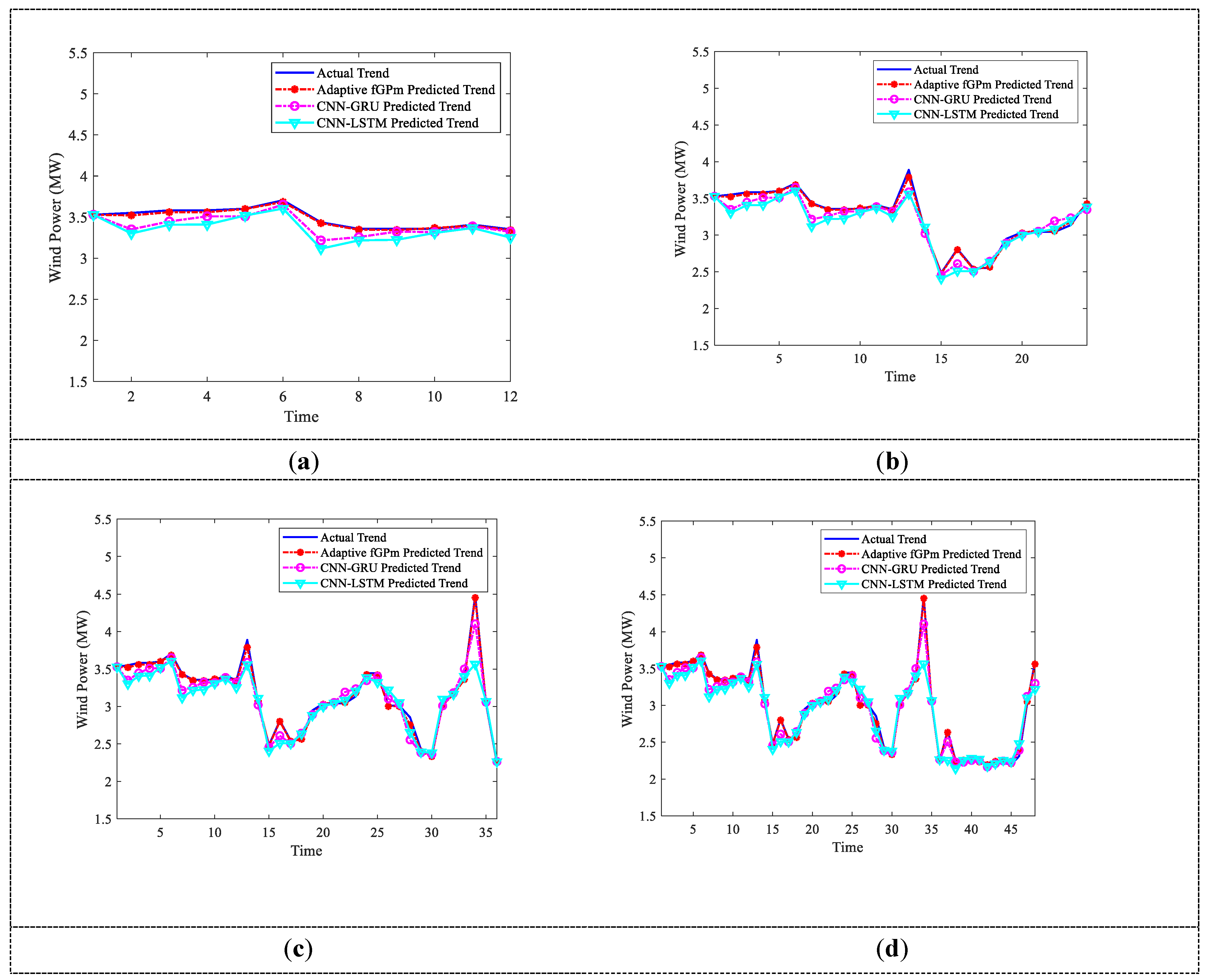
To substantiate the superior predictive accuracy of the proposed model, it was compared with the FBm and CNN-GRU models. Historical data, including Numerical Weather Prediction (NWP) and power output data, were collected on December 26, 2019 (winter), from 7:00 to 19:00, and on July 12, 2019 (summer), during the same hours. Samples were taken every 30 minutes to forecast the wind power output for intervals of 6, 12, 18, and 24 hours ahead. The comparative results are depicted in Figure 8 and Figure 9.
The comparative analysis from Figure 8 and Figure 9 reveals that the power output of wind farms is generally higher in winter than in summer. This phenomenon can likely be attributed to the greater variability in wind speed during the winter months, which in turn leads to a significant increase in the volatility of wind power output. All models have demonstrated a satisfactory fit in simulating the actual wind power curves. However, when confronted with sampling points where there are sharp changes in wind speed, the adaptive fGPm model proposed in this study, with its capability to capture long-range dependencies, shows a notably significant advantage in predictive accuracy. By conducting an in-depth analysis of the data, this model significantly enhances the consistency between predicted and observed values, achieving a high degree of accuracy in fitting the wind power curve. In contrast, the CNN-LSTM model exhibits relatively larger predictive errors at some sampling points, indicating a potential need for further optimization in handling such extreme fluctuations.This refined translation maintains the original message's intent while enhancing the language for a professional and academic context.

5.5.2. Performance Comparison of Different Models

In the performance comparison of various models, the evaluative indicators presented in Table 3 indicate that the Adaptive Fractional Gaussian Process Regression (fGPm) model demonstrates superior performance over the CNN-GRU and CNN-LSTM models in two pivotal metrics: Root Mean Square Error (RMSE) and Mean Absolute Percentage Error (MAPE). The RMSE of the Adaptive fGPm model exhibits an average decrease of 0.448MW and 0.466MW relative to the CNN-GRU and CNN-LSTM models, respectively. Additionally, the MAPE has seen an average reduction of 6.936% and 9.702%, respectively. This significant improvement in performance is mainly due to two key aspects: First, the model's adaptive drift coefficient dynamically adjusts to incoming data, more accurately reflecting the trends in wind power variations. Second, by effectively harnessing the long-range dependence (LRD) features of time series data, the model distills overall characteristics and accentuates the importance of critical input information, which substantially improves the precision of the forecasts.

6. Conclusions

The adaptive fractional-order generalized Pareto motion (fGPm) iterative differential forecasting method proposed in this study demonstrates superior performance and high accuracy in short-term wind power forecasting, showcasing significant practical application potential. The main conclusions are as follows:
Key Role of Data Processing: To address the impact of the complex temporal characteristics of wind power generation on model accuracy, we employed the Orthogonalized Maximum Information Coefficient feature selection method. This significantly enhanced the correlation between wind power and the selected features, validating the effectiveness of the feature extraction approach.
Long-Range Dependence (LRD) Characteristics of Wind Power Series: By analyzing the relationship between the Hurst parameter and feature indices, we revealed the LRD characteristics of wind power series. This finding provides a theoretical basis for modeling with the adaptive fGPm, particularly improving trend prediction accuracy under optimized sample lengths and forecasting horizons.
Parameter Estimation of New Feature Function Method: We successfully applied a new feature function method to estimate parameters such as stability index, skewness index, drift coefficient, and diffusion parameter within the adaptive fGPm model, laying a solid foundation for building a reliable forecasting model.
Superiority of the Adaptive fGPm Forecasting Model: The adaptive fGPm iterative differential forecasting model effectively addresses uncertainties in wind power generation by introducing tail parameters, thereby enhancing the flexibility of LRD characterization. This model demonstrated advantages in forecasting high-volatility data, with its diffusion coefficient adapting to environmental changes to more accurately reflect dynamic wind power characteristics.
Comparison with Other Models: Comparative analyses with mainstream forecasting models such as CNN-GRU and CNN-LSTM demonstrated the superiority and versatility of the adaptive fGPm model in describing wind power data, achieving higher prediction accuracy.
In summary, This research provides an innovative adaptive fGPm iterative differential forecasting model for accurate short-term wind power predictions, aiding power departments in optimizing generation planning and scheduling. Furthermore, it serves as an effective reference for other time series forecasting scenarios, such as wind speed, photovoltaic generation, and precipitation.

Author Contributions

F.C.: conceptualization, methodology, software, writing—original draft. writing—review and editing, methodology. T.Z.: formal analysis, data curation. Y.J.: Project administration, Resources, Supervision. D.Ch..: Funding acquisition, Supervision, Software. All authors have read and agreed to the published version of the manuscript.

Funding

This work was supported by the Science and Technology Project of Quanzhou City under Grant 2024QZC004R, and the Natural Science Foundation of Fujian Province under Grant 2024J01208. and the Science and Technology Project of Fujian Province under Grant 2023H6026.

Data Availability Statement

Wind farms have confidentiality requirements regarding their data, and we cannot publish the data we have used.

Acknowledgments

The authors would like to thank the anonymous reviewers who gave valuable suggestions that have helped to improve the quality of the manuscript.

Conflicts of Interest

The authors declare no conflicts of interest.

References

  1. Li, Y.; Sun, C.; Jiang, Y.; Feng, F. Scaling Method of the Rotating Blade of a Wind Turbine for a Rime Ice Wind Tunnel Test. Energies 2019, 12, 627.
  2. Thango,B.A.;Bokoro,P.N.Prediction of the Degree of Polymerization in Transformer Cellulose Insulation Using the Feedforward Backpropagation Artificial Neural Network.Energies 2022, 15, 4209.
  3. Ju, Y.;Sun, Y.; Chen,Q.A model combining convolutional neural network and LightGBM algorithm for ultra-short-term wind power forecasting.IEEE Access, 2019, 7,28309-28318.
  4. Zhao, Y. B.;Guo, N.; Chen,W. Multi-step ahead forecasting for electric power load using an ensemble model. Expert Systems with Applications. 2023, 211, 118649.
  5. Li, Y.; Wu,Z.; Su,Y. Adaptive Short-term Wind Power Forecasting Based on Feature Extraction and Fuzzy Gaussian Process Regression.Renewable Energy. 2023,217 ,119146.
  6. Cai, H.; Jia,X.; Feng,J. A combined filtering strategy for short term and long term wind speed prediction with improved accuracy.Renewable Energy. 2019, 136,1082-1090.
  7. Wang, J.; Tang, X.D. An intensive decomposition integration paradigm for short-term wind power forecasting based on feature extraction and optimal weighted combination strategy. Measurement 2023,223,113811.
  8. Lu,P. Short-term wind power forecasting based on meteorological feature extraction and optimization strategy. Renewable Energy.2022,184,642-661.
  9. Liao, S.; Tian, X.; Liu, B.; Liu, T.; Su, H.; Zhou, B. Short-Term Wind Power Prediction Based on LightGBM and Meteorological Reanalysis. Energies.2022, 15, 6287. [CrossRef]
  10. Wang,Y. S.;Gao, J.; Xu,Z.W.; Luo,J.D.;Li,L.X.A Prediction Model for Ultra-Short-Term Output Power of Wind Farms Based on Deep Learning.International Journal of Computers Communications.2020,15,3901. [CrossRef]
  11. Sun,Z.X.;Zhao,M.Y.Short-term wind power forecasting based on VMD decomposition, ConvLSTM networks and error analysis.IEEE Access.2020,8,134422-134434.
  12. Lu,P.Feature extraction of meteorological factors for wind power prediction based on variable weight combined method.Renewable Energy.2021,179,1925-1939.
  13. Yang, G. H.;Qi, X.;Jia, R.;Liu, Y. F.;Meng, F.;Ma, X.;Xing, X. W.Short-term wind power prediction based on CEEMD-SE, CNN&LSTM-GRU. Electric Power,2024 ,57(2), 55-61.
  14. Ji, J.; Wang, D.; Xu, D.; Xu, C. Combining a self-exciting point process with the truncated generalized Pareto distribution: An.
  15. extreme risk analysis under price limits. J. Empir. Financ. 2020, 57, 52–70. [CrossRef]
  16. Lahiri, S.N.; Das, U.; Nordman, D.J. Empirical Likelihood for a Long Range Dependent Process Subordinated to a Gaussian Process. J. Time Ser. Anal. 2019, 40, 447–466. [CrossRef]
  17. Lu,Peng.;Ye,Lin.; Pei, M.; Zhao, Y.N.Short-term wind power forecasting based on meteorological feature extraction and optimization strategy.Renewable Energy.2022,184,642-661. [CrossRef]
  18. Wu, Yuan-Kang.Deterministic and probabilistic wind power forecasts by considering various atmospheric models and feature engineering approaches.IEEE Transactions on Industry Applications.2022,59, 192-206.
  19. Noorollahi,Y.;Mohammad.A.J.;Ahmad,K.Using artificial neural networks for temporal and spatial wind speed forecasting in Iran,Energy Conversion and Management.2016,115,17-25. [CrossRef]
  20. Chen,Y.J.;Xiao,J.W.;Wang,Y.W.; Li,Y.Regional wind-photovoltaic combined power generation forecasting based on a novel multi-task learning framework and TPA-LSTM.Energy Conversion and Management,2023, 297,117715.
  21. Razin,Ahmed.;Victor,Sreeram.;Roberto,Togneri.;Amitava Datta.;Muammer Din Arif.Computationally expedient Photovoltaic power Forecasting: A LSTM ensemble method augmented with adaptive weighting and data segmentation technique,Energy Conversion and Management.2022,258,115563. [CrossRef]
  22. Ali,A.; Ahmed,A.; Moussa,L.; Yassine,E.H.Short-term self consumption PV plant power production forecasts based on hybrid CNN-LSTM, ConvLSTM models.Renewable Energy.2021,177,101-112.
  23. Zhang,W.; Cai,Y.; Zhan,H.Y.;Yang,M.;Zhang,Wei.Multi-energy load forecasting for small-sample integrated energy systems based on neural network Gaussian process and multi-task learning.Energy Conversion and Management,2024,321,119027.
  24. Li,Chuang.;Li,G.J.;Wang,K.Y.;Han,B.A multi-energy load forecasting method based on parallel architecture CNN-GRU and transfer learning for data deficient integrated energy systems.Energy.2022,259,124967.
  25. Ge, R.;Zhou, M.;Luo, Y.McTwo:a two-step feature selection algorithm based on maximal information coefficient. BMC Bioinformatics .2016,17, 142. [CrossRef]
  26. Han,Y.; Mi,L.H.;Shen,L.;Cai,C.S.;Liu,Y.C.;Li,K.;Xu,G.J.A short-term wind speed prediction method utilizing novel hybrid deep learning algorithms to correct numerical weather forecasting.Applied Energy.2022,312,118777.
  27. Marquardt, T. Fractional Lévy processes with an application to long memory moving average processes. Bernoulli 2006, 12, 1099–1126.
  28. Chen,J.; Liu,H.;Chen,C.;Zhu,D.Wind speed forecasting using multi-scale feature adaptive extraction ensemble model with error regression correction.Expert Systems with Applications.2022, 207,117358. [CrossRef]
  29. Lim, S.; Li, M. A generalized Cauchy process and its application to relaxation phenomena. J. Phys. A Math. Gen. 2006, 39, 2935–2951. [CrossRef]
  30. Li, M.; Li, J.Y. Generalized Cauchy model of sea level fluctuations with long-range dependence. Phys. A Stat. Mech. Its Appl. 2017, 484, 309–335. [CrossRef]
  31. Dou,C.;Zheng,Y.;Yue,D.;Zhang,Z.;Ma,K.Hybrid model for renewable energy and loads prediction based on data mining and variational mode decomposition. IET Gener,Transmiss. Distrib.2018, 12, 2642–2649.
  32. Cao,B.; Chang,L. Development of Short-Term Wind Power Forecasting Methods. 2022 IEEE 7th Southern Power Electronics Conference (SPEC), Nadi, Fiji, 2022, 1-5. [CrossRef]
  33. Feng,C.;Cui,M.;Hodge,B.M.;Zhang,J.A data-driven multi-model methodology with deep feature selection for short-term wind forecasting.Applied Energy.2017,190, 1245-1257.
  34. A,Kisvari.;Z,Lin.;Liu,X.Wind power forecasting-a data-driven method along with gated recurrent neural network. Renewable Energy.2021, 163, 1895-1909.
  35. Li,L.;Zhang,Z.; Zhang,S.;Hybrid algorithm based on content and collaborative filtering in recommendation system optimization and simulation.Sci. Program. 2021,7427409.1–7427409.11.
  36. Yang,Z.;Zhou,F.;Yang,L.;Zhang,Q.A new prediction method for recommendation system based on sampling reconstruction of signal on graph.Expert Syst. Appl. 2020,159, 113587.1–113587.12. [CrossRef]
  37. Carrillo, R.E.; Aysal, T.C.; Barner, K.E. A generalized Cauchy distribution framework for problems requiring robust behavior. EURASIP J. Adv. Signal Process. 2010, 312989. [CrossRef]
  38. Liu, H.; Song, W.; Zio, E. Generalized Cauchy difference iterative forecasting model for wind speed based on fractal time series. Nonlinear Dyn. 2021, 103, 759–773.
  39. Liu, H.; Song, W.Q.; Zio, E. Fractional Lévy stable motion with LRD for RUL and reliability analysis of li-ion battery. ISA Trans. 2022, 125, 360-370.
  40. Kogon, S.M.; Manolakis, D.G. Signal modeling with self-similar α -stable processes: The fractional levy stable motion model. IEEE Trans. Signal Process. 1996, 44, 1006–1010.
  41. Song, W.; Liu, H.; Zio, E. Long-range dependence and heavy tail characteristics for remaining useful life prediction in rolling bearing degradation. Appl. Math. Model. 2022, 102, 268–284.
  42. Song, W.Q.; Duan, S.W.; Chen, D.D.; Zio, E.; Yan, W.D.; Cai, F. Finite Iterative Forecasting Model Based on Fractional Generalized Pareto Motion. Fractal. Fract. 2022, 6, 471.
  43. Ramirez, J.A.; Echeverria, J.C.; Rodriguez, E. Performance of a high-dimensional R/S method for Hurst exponent estimation. Phys. A.2008, 387, 6452–6462.
  44. Jie,X.;Song, W.Q.; Francesco, V. Generalized Cauchy Process: Difference Iterative Forecasting Model. Fractal Fract. 2021, 5, 38. [CrossRef]
  45. Savović,S.;Djordjevich,A.Investigation of Mode Coupling in Graded Index Plastic Optical Fibers Using the Langevin Equation. in Journal of Lightwave Technology. 2020.38,6644-6647.
  46. Sayah, M.; Guebli, D.; Masry, Z.A.; Zerhoui, N. Robustness testing framework for RUL prediction Deep LSTM networks. ISA Trans. 2021, 113, 28–38. [CrossRef]
  47. Wang,Y.;Zou,R.;Liu,F.;Zhang,L.J.;Liu,Q.Y.A review of wind speed and wind power forecasting with deep neural networks.Applied Energy.2021,304,117766. [CrossRef]
  48. Zheng,J.Q.;Du,J.;Wang,B.H.;Jiří Jaromír Klemeš.;Liao,Q.;Liang,Y.T.A hybrid framework for forecasting power generation of multiple renewable energy sources.Renewable and Sustainable Energy Reviews.2023, 172,113046.
  49. Zhang,J.H.;Yan,J.;Liu,Y.Q.;Lin,F.S.Short-term forecasting and uncertainty analysis of wind turbine power based on long short-term memory network and Gaussian mixture model.Applied Energy.2019,241,229-244.
  50. Jiang,M.;He,Y.;Zhang,T.;Yang, B.Wind Power Prediction Based on Feature Selection and Error Correction. Distributed Energy.2023,8(2), 37-43. [CrossRef]
  51. Ma, Z.;Zhang, L.;Ba, Y.;Xie, M.;Zhang, P.;Wang, X.Ultra-Short-Term Wind Power Prediction Based on Adaptive Quadratic Mode Decomposition and CNN-BiLSTM. Solar Energy. 2024, 228, 1-10. [CrossRef]
  52. Chen,Y.;Li,Y.;Li,H.Ultra-Short-Term Prediction of Wind Power Based on VMD-PE-MulitiBiLSTM. Distributed Energy.2024,9(2), 1-7. [CrossRef]
  53. Wu, X.; Liang, X.; Zhu, H.; Zhang, D. Short-term Wind Power Prediction Based on CEEMDAN-GRA-PCC-ATCN. Journal of Guangxi University (Engineering Edition).2022,42(6), 1-9.
  54. Liu,J.J.;Wang,J.Z.;Niu,Y.B.;Ji,B.Q.;Gu,L.A point-interval wind speed forecasting system based on fuzzy theory and neural networks architecture searching strategy. Engineering Applications of Artificial Intelligence,2024, 132,107906.
  55. Hodge,B.M.;Zeiler,A.;Brooks,D.C.;Blau,G.;Joseph Pekny.; Gintaras Reklatis.Improved Wind Power Forecasting with ARIMA Models.Computer Aided Chemical Engineering 2011, 29, 1789-1793. [CrossRef]
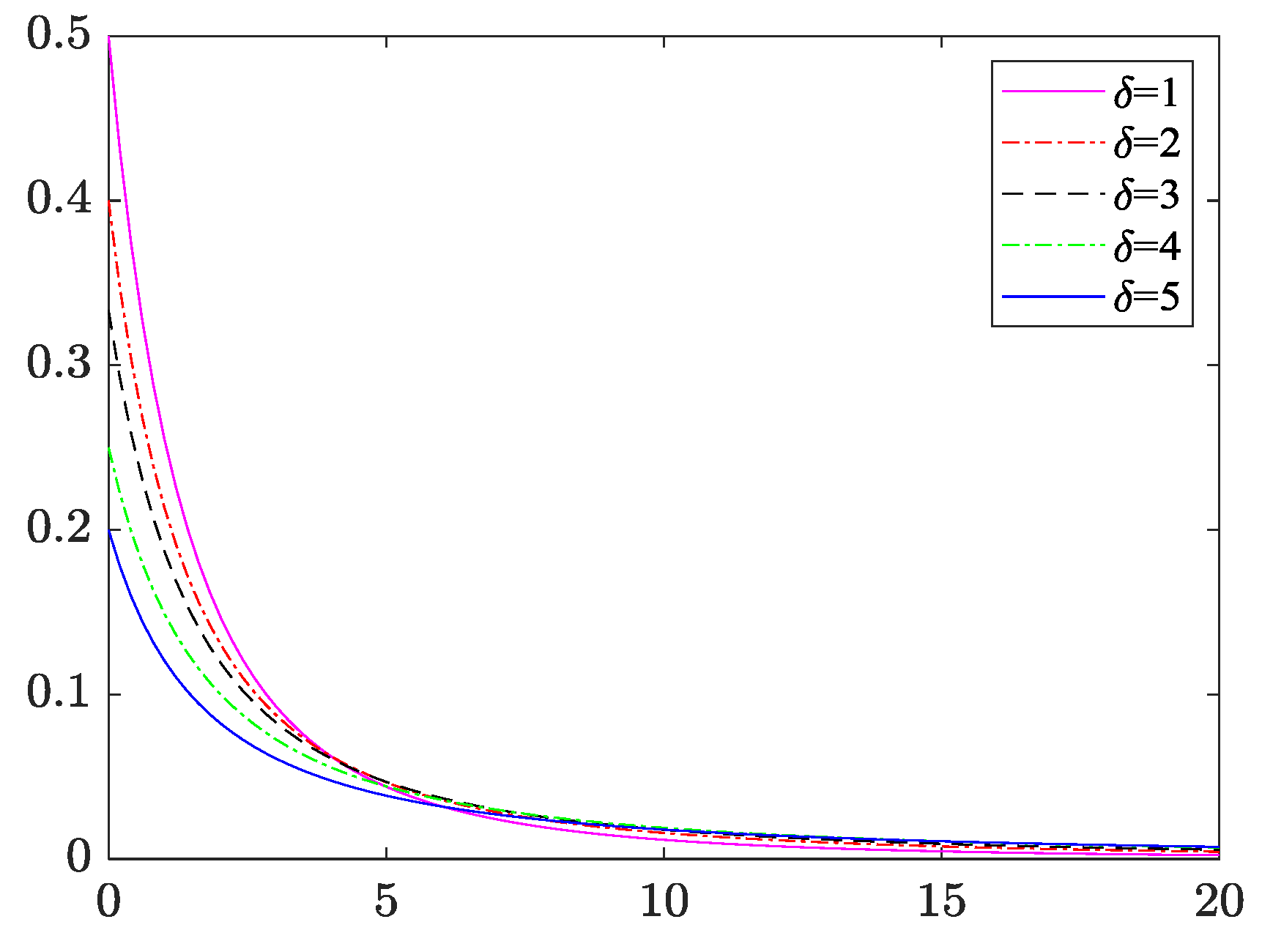
Figure 1. Probability Density Distribution of GPD with Different Shape Parameters.
Figure 2. Probability Density Distribution of GPD with Different Scale Parameters.
Preprints 121043 g001
Figure 3. Simulation sequences of the fGPm model under different conditions (a) H = 0.85, α = 1.1 ; (b) H = 0.85, α = 1.4 ; (c) H = 0.85, α = 1.7 ; (d) H = 0.85, α = 2 . Time representation in the figure is specified as time steps, where each time step represents the simulated sequence count.
Preprints 121043 g002
Figure 4. Original Wind Power Data.
Preprints 121043 g003
Figure 5. Wind farm power generation forecasting model framework.
Preprints 121043 g004
Figure 6. Winter Wind Power Forecasting Results for Wind Turbine Generators; (a) predicting 12 steps; (b) predicting 24 steps; (c) predicting 36 steps; (d) predicting 48 steps.
Preprints 121043 g005aPreprints 121043 g005b
Figure 7. Summer Wind Power Forecasting Results for Wind Turbine Generators; (a) predicting 12 steps; (b) predicting 24 steps; (c) predicting 36 steps; (d) predicting 48 steps.
Preprints 121043 g006aPreprints 121043 g006b
Figure 8. Comparison of Prediction Curves from Different Models in Winter.(a) 6 h (b) 12 h (c) 18 h (d) 24 h.
Preprints 121043 g007
Figure 9. Comparison of Prediction Curves from Different Models in Summer.(a) 6 h (b) 12 h (c) 18 h (d) 24 h.
Preprints 121043 g008
Table 1. Forecasting Model Parameter Estimation
H α μ δ
Case 1 0.8315 1.7142 640.2534 3.1201
Case 2 0.7915 1.7235 750.4211 2.6617
Table 2. Forecast Model Performance Analysis.
Season Forecast Length Evaluation Metrics
RMSE(MW) MAPE(%) R 2


Winter
12 0.842 22.456 0.9614
24 1.141 23.412 0.9721
36 1.021 25.321 0.9717
48 1.332 26.334 0.9711


Summer
12 0.772 5.047 0.9750
24 0.956 5.678 0.9711
36 1.121 6.123 0.9817
48 1.242 7.123 0.9830
Table 3. Comparative Analysis of Forecasting Results Across Various Models.
Season Prediction time CNN-GRU CNN-LSTM Adaptive fGPm
RMSE(MW) MAPE(%) RMSE(MW) MAPE(%) RMSE(MW) MAPE(%)


Winter
6h 0.887 30.321 1.223 37.125 0.505 19.231
12h 0.997 31.151 1.321 38.243 0.609 20.421
18h 1.552 32.321 1.421 39.354 0.891 21.504
24h 1.921 33.256 1.521 40.321 0.997 22.022


Summer
6h 0.778 7.126 0.899 8.121 0.231 5.231
12h 0.887 8.326 0.951 8.231 0.401 4.355
18h 0.901 8.541 0.996 9.332 0.586 5.501
24h 0.998 9.231 1.211 9.512 0.799 6.521
Average 1.115 20.034 1.193 23.800 0.627 13.098
Disclaimer/Publisher’s Note: The statements, opinions and data contained in all publications are solely those of the individual author(s) and contributor(s) and not of MDPI and/or the editor(s). MDPI and/or the editor(s) disclaim responsibility for any injury to people or property resulting from any ideas, methods, instructions or products referred to in the content.
Copyright: This open access article is published under a Creative Commons CC BY 4.0 license, which permit the free download, distribution, and reuse, provided that the author and preprint are cited in any reuse.
Prerpints.org logo

Preprints.org is a free preprint server supported by MDPI in Basel, Switzerland.

Subscribe

© 2024 MDPI (Basel, Switzerland) unless otherwise stated