Stochastic Models for Ontogenetic Growth

Preprint

Article

Stochastic Models for Ontogenetic Growth

Altmetrics

Downloads

Views

Comments

A peer-reviewed article of this preprint also exists.

This version is not peer-reviewed

Submitted:

14 October 2024

Posted:

15 October 2024

You are already at the latest version

Alerts

Abstract

Based on allometric theory and scaling laws, numerous mathematical models have been proposed to study ontogenetic growth patterns of animals. Although deterministic models have provided valuable insight into growth dynamics, animal growth often deviates from strict deterministic patterns due to stochastic factors such as genetic variation and environmental fluctuations. In this study, we extend a general model for ontogenetic growth proposed by West et al. to stochastic models for ontogenetic growth by incorporating stochasticity using white noise. According to data variance fitting for stochasticity, we propose two stochastic models for ontogenetic growth, one is for determinate growth and one is for indeterminate growth. To develop a universal stochastic process for ontogenetic growth across diverse species, we approximate stochastic trajectories of two stochastic models and apply random time change and obtain a geometric Brownian motion with a multiplier of an exponential time factor. We conduct detailed mathematical analysis and numerical analysis for our stochastic models. Our stochastic models predict well not only average growth, but also variations of growth within species. This stochastic framework may be extended to studies of other growth phenomena.

Keywords:

Subject: Computer Science and Mathematics - Applied Mathematics

1. Introduction

The ontogenetic growth pattern has been a fascinating research topic in history. Based on individual growth data sets, previous researchers scaled the time to “physiological time”to obtain ontogenetic growth curves [1,2]. Von Bertalanffy proposed a first mathematical model to describe individual growth [3,4]. Specifically, the rate of change in body mass is equal to the rate of acquisition of nutrients and energy by the growing individual minus the maintenance requirement of accumulated tissue, with appropriate parameters for converting inputs to body mass, the growth rate and maintenance rate. Von Bertalanffy assumed that tissue maintenance would be proportional to mass but that nutrient provisioning would follow a surface rule and increase with the

\frac{2}{3}

power of mass. After this, several subsequent ontogenetic growth models have been proposed [5,6,7]. Most of these models are derived from metabolic scaling theory or allometric theory and fitted with specific species data sets. The growth rate is observed to vary considerably between species and is less variable within species [8,9,10]. West et al. proposed a general ontogenetic growth model [11]. Rather than provision nutrients with the mass power

\frac{2}{3}

, this general model assumes the scaling exponent

\frac{3}{4}

for energy acquisition with respect to mass [12,13]. Makarieva et al. extended this model to incorporate energy conservation in ontogenetic development [14]. There are also other modifications of the general ontogenetic growth model [15]. Hou et al. developed a general model for ontogenetic growth under food restriction [16]. Shi et al. compared several ontogenetic models for crop growth [17]. Based on metabolic scaling and fitting of fish data, Sibly et al. estimated that the scaling exponent for energy acquisition is in the range

0.65 - 0.77

[18]. Hatton et al. conducted a comprehensive study on scaling and body mass [19]. Recently, Escala used the heart frequency to define a time scale for ontogenetic growth that can recover a general ontogenetic growth model [20].

All these mathematical models for ontogenetic growth have useful and explanatory powers. However, these mathematical models were estimated on the basis of partial information provided by their data sets. All of them do not fully utilize the data sets in their modeling studies. We may say that the data fitting was only fitted for averages of the data sets, and so solutions or solution curves at most were an approximation of averages of the data sets. The only information from the data sets that was used for the construction of the model was the averages of the data sets. There are other data sets information that was not used. For example, the variances of the data sets were not used in all these studies. For the variance of a data set of an individual growth, the variance can be considered as a result of environmental uncertainty, environmental noise, or environmental stochastic factors. Variances may also be interpreted as variations among individuals within a species. In this study, we seek to incorporate more information provided by data sets into mathematical models for ontogenetic growth. Ito’s stochastic differential equations are a good mathematical device to handle both averages and variances when building mathematical models. There is a study that applied a stochastic differential equation for ontogenetic growth [21]. Unfortunately, it is difficult to interpret its linear noise term as data variances.

In the research of a general ontogenetic growth model [11], the authors proposed two types of growth patterns, determinate growth and indeterminate growth. However, the mathematical model itself cannot distinguish these two patterns, and there was no mathematical character that could distinguish these two growth patterns. In the present study, we construct stochastic models for ontogenetic growth in terms of stochastic differential equations. It turns out that our stochastic model is capable of distinguishing determinate growth from indeterminate growth.

The rest of the article is organized as follows. In Section 2, we recall the general model for ontogenetic growth proposed by West et al. Based on the data sets in [11], we propose two stochastic models for ontogenetic growth, one for determinate growth and one for indeterminate growth. In Section 3, we perform parameter estimation and model fitting. Firstly, we fit the average growth trajectory to a deterministic curve. Secondly, we incorporate stochasticity by identifying the best-fitted white noise term to represent growth variance. By combining these two fits, we obtain stochastic differential equation models that improve the prediction of growth trajectories, capturing the variability of ontogenetic growth. In Section 4, we provide rigorous mathematical analysis for our stochastic models. In Section 5, we make some approximations for our stochastic models and obtain a universal stochastic growth process. The article ends with a discussion section, where we propose some interesting questions and give some new perspectives on the research field.

2. Mathematical Model Setup

2.1. General Deterministic Model for Ontogenetic Growth

In this subsection, we recall the deterministic models for ontogenetic growth. We focus on a general ontogenetic growth model proposed by West et al. [11]. This model is quantitatively based on fundamental principles that at any time

t > 0

, the average resting metabolic rate of an entire organism, denoted by B, can be expressed as a sum of two components:

B = \sum_{c} [N_{c} B_{c} + E_{c} \frac{d N_{c}}{d t}] .

(1)

Here,

N_{c}

is the total number of cells,

B_{c}

accounts for energy for the maintenance of an existing cell, and

E_{c}

corresponds to the energy for the creation of a single new cell. Under the assumption that any potential variations between cells are ignored, a typical average cell mass is considered the fundamental unit

m_{c}

. Furthermore, it is assumed that all

E_{c}

B_{c}

, and

m_{c}

are independent of total biomass m, and remain constant throughout growth and development processes. At any time t, we assume that

m : = m (t) = m_{c} N_{c}

where

N_{c} = N_{c} (t)

is the function of time t that represents the total number of cells of a species over time. Then equation (1) can be written as

\frac{d m}{d t} = (\frac{m_{c}}{E_{c}}) B - (\frac{B_{c}}{E_{c}}) m

(2)

Now, if we allow the relation

B = B_{0} m^{3 / 4}

to be adopted where

B_{0}

is a constant for a given species, then the equation (2) can be rewritten as

\frac{d m}{d t} = a m^{3 / 4} [1 - {(\frac{m}{M})}^{1 / 4}],

(3)

where

a = B_{0} m_{C} / E_{C}

is the combined parameter, which represents the growth rate of a species, and

m = m (t)

is the variable that represents the total biomass of a species at time t. Supported by extensive data on mammals, birds, fish, mollusks and plants, the 3/4-power scaling, attributed to “growth spurts”, characterizes the general allometry of B from birth to reproductive maturity. The model provides the basis for deriving an allometric relationship for growth rates and the timing of life-history event. The different exponents of m in the two terms on the right-hand side of

()

demonstrate the mechanism that the network restricts the total number of supply units to scale differently from the total number of cells supplied. This imbalance between supply and demand ultimately limits growth, and therefore, with the growth rate a, an asymptotic maximum body size M is reached. Let

m_{0}

denote the initial mass of the organism at birth. Integration of the equation results in a classical sigmoidal curve, illustrating the growth trajectory of the organism over time,

m (t) = M {\{1 - [1 - {(\frac{m_{0}}{M})}^{1 / 4}] e^{- a t / 4 M^{1 / 4}}\}}^{4}

(4)

The parameters a,

m_{0}

, and M vary between species. In their study, they estimated these parameters for 13 species from various taxons, including mammals, birds, fish, and crustaceans, and showed that the growth trajectories of all these species align with the deterministic curves

()

. From data analysis, the authors proposed two growth patterns: determinate growth, which attains the maximum size at a certain point in their lifespan and ceases growing, and indeterminate growth, which never reach the maximum size and exhibit a continuous growth throughout their life span. Furthermore, the solution curves seem to suggest some potential frameworks for visualizing data beyond individual species, unveiling universal growth properties across taxonomic groups.

2.2. Stochastic Models for Ontogenetic Growth

Our objective is to improve the accuracy of the model in representing growth dynamics in diverse species of animals. In practical scenarios, animal growth does not adhere solely to deterministic principles, and stochasticity plays a significant role in shaping outcomes. Factors such as genetic variation, environmental factor fluctuations, and chance events introduce randomness into growth processes. Therefore, incorporating stochastic elements into the model will enable us to create enhanced models that more faithfully reflect the complexities of nature, enhancing our understanding of animal growth dynamics, and improving our ability to predict and manage biological systems in a variety of contexts.

Now, let us start with the equation (3). To facilitate the complexity of this equation, we introduce the variable

R (t) = 1 - {(m (t) / M)}^{1 / 4}

which stands for the relative proportion of total available metabolic energy expended on growth of a species. Then differentiating

R (t)

and using equation (3) give us the following simple equation.

d R (t) = - \frac{a}{4 M^{1 / 4}} R (t) d t .

(5)

Noise is well known in the process of energy transformation and the variation in metabolic energy expenditure during cell growth is a key factor influencing the diversity of growth patterns. Observe that growth parameters a and M vary among different species and also carry “noises”. Therefore, we aim to represent this variation by perturbing the ratio of these two parameters with white noise. The question is how to find a good representation for the noise intensity.

We tackle this question by examining the impact of noise through studying the significant proportion of total metabolic energy allocated to growth throughout an organism’s lifetime. To facilitate the following process, we introduce the variable

r (t) = 1 - R (t) = {(m (t) / M)}^{1 / 4}

that represents the relative proportion of the total available metabolic energy that fuels the maintenance of a species. Suppose

0 < t_{d}

represents the death time of a species. Whether the individual exhibits determinate or indeterminate growth, under the assumption that in initiation most of the energy is allocated to cell growth and metabolic energy for cell maintenance is ignored, the total metabolic energy

E_{t o t}

expended since birth to a time

0 < t < t_{d}

can be calculated by integrating B up to that time. The details are as follows:

\begin{matrix} E_{t o t} & = \int_{0}^{t} B (s) d s = \int_{0}^{t} B_{0} m^{3 / 4} (s) d s = \int_{0}^{t} B_{0} r {(s)}^{3} M^{3 / 4} d s \\ = \int_{0}^{t} B_{0} r {(s)}^{3} M^{3 / 4} \cdot \frac{4 M^{1 / 4}}{a} \cdot \frac{d r (s)}{1 - r (s)} = \frac{4 B_{0} M}{a} \int_{0}^{t} \frac{r {(s)}^{3}}{1 - r (s)} d r (s) \\ = \frac{4 B_{0} M}{a} [- \frac{1}{3} r {(s)}^{3} - \frac{1}{2} r {(s)}^{2} - r (s) - ln (1 - r (s))] |_{0}^{t} \\ \approx \frac{4 B_{0} M}{a} [- \frac{1}{3} r^{3} (t) - \frac{1}{2} r {(t)}^{2} - r (t) - ln (1 - r (t))] . \end{matrix}

Meanwhile, the allocation of resources to support cell growth within the same time frame depends on how the rate of change of total cell counts in the organism evolves over time. This allocation can be determined by examining the following integral

\begin{matrix} E_{g} = \int_{0}^{t} E_{C} (\frac{d N_{C}}{d t}) d t = \int_{0}^{t} \frac{E_{C}}{m_{C}} d m & = \frac{B_{0}}{a} \frac{E_{C}}{m_{C}} (m (t) - m_{0}) \approx \frac{B_{0} M}{a} r^{4} (t) . \end{matrix}

Consequently, considering that the mass ratio remains within a range between 0 and 1 for any time

t \geq 0

, we can examine the ratio of two quantities

E_{t o t}

and

E_{g}

\begin{matrix} \frac{E_{g}}{E_{t o t}} & \approx \frac{r^{4} (t)}{4 [- \frac{1}{3} r^{3} (t) - \frac{1}{2} r^{2} (t) - r (t) - ln (1 - r (t))]} \\ \leq \frac{1 / 4}{1 - r (t) + min [- 1 - ln (1 - r (t)) - \frac{1}{3} r^{3} (t) - \frac{1}{2} r^{2} (t)]} \\ = \frac{1 / 4}{R (t) + min [- 1 - ln (R (t)) - \frac{1}{3} r^{3} (t) - \frac{1}{2} r^{2} (t)]} . \end{matrix}

(6)

For a species, the energy ratio

E_{g} / E_{t o t}

represents the percentage of its total energy in life that is spent on cell growth. This ratio should be different for different species. From the growth data set of 13 species in [11], we observed that there are 3 species (Salmon, Cod, and Shrimp) belonging to indeterminate growth type and the remaining 10 species belonging to determinate growth type. From the fitted results in [11], it is noticeable that the indeterminate group has a much smaller fitted growth rate a and birth biomass

m_{0}

. Thus, the data variation in this group is much smaller than that in determinate group. Because of this, we adopt two functions

g_{1} (R)

and

g_{2} (R)

to represent the intensity of noise for the determinate and indeterminate groups, respectively. The forms of these two functions are based on the ratio

E_{g} / E_{t o t}

, since it can estimate the intensity of noise in the percentage of energy expended for cell growth during energy transformation.

For simplicity, first we approximate the right-hand side of inequality (6) with a function of the form

g_{1} (R) = σ / (δ + R)

for the determinate group, where

σ

and

δ

are some constants that keep the inequality right. Therefore, we adopt the function

g_{1} (R)

to represent the intensity of noise in the determinate group and introduce the following perturbation method to the growth rate ratio

\frac{- a}{4 M^{1 / 4}} \to \frac{- a}{4 M^{1 / 4}} + g_{1} (R (t)) \frac{d W (t)}{d t},

where

W (t)

is a standard Wiener process. With this setup, equation

()

becomes a stochastic differential equation that describes the dynamics of the proportion of energy expended for cell growth in determinate group

d R (t) = \frac{- a}{4 M^{1 / 4}} R (t) d t + \frac{σ R (t)}{δ + R (t)} d W (t) .

(7)

Taking into account that the five parameters a, M,

m_{0}

σ

and

δ

vary between different species in the determinate group. For the indeterminate group, since this group shows a smaller data variation compared with the determinate group, we adopt the function

g_{2} (R) = σ (1 - R) / (δ + R)

to represent the noise intensity in the indeterminate group. Then we incorporate this function into the growth rate ratio as follows

\frac{- a}{4 M^{1 / 4}} \to \frac{- a}{4 M^{1 / 4}} + g_{2} (R (t)) \frac{d W (t)}{d t} .

This leads to another stochastic differential equation that describes the dynamics of the proportion of energy used for cell growth in the indeterminate group

d R (t) = \frac{- a}{4 M^{1 / 4}} R (t) d t + \frac{σ R (t) [1 - R (t)]}{δ + R (t)} d W (t) .

(8)

In Section 4, we will analyze theoretically these two stochastic equations (7) and (8) and explain why we choose these two equations for understanding the data set of 13 species in [11] from mathematical point of view. In the next section, we will showcase how to fit the growth data set of 13 species using two proposed stochastic differential equations.

3. Parameter Fitting

3.1. Dataset

In this study, we used a diverse data set consisting of 206 samples collected from a wide range of animal species, encompassing 13 different types, including mammals, birds, fish, and crustaceans. The species represented in the data set are Guppy, Heron, Hen, Salmon, Rat, Atlantic Cod, Robin, Shrew, Guinea Pig, Domestic Rabbit, Domestic Pig, Cow and Shrimp. These species were chosen to provide a comprehensive representation of various growth patterns that include both determinate and indeterminate growth. The data set provides measurements of time (denoted as t and reported in days) and organism size (denoted as m and reported in grams). Time serves as the independent variable, representing the duration of growth observation, while the size of the organism serves as the dependent variable, representing the size of the organism at each time point.

3.2. Fitting Method

We start with the relative rate of change

\frac{\dot{R}}{R}

in the proportion of energy expended on growth of a species. Then we allow

\frac{\dot{R}}{R} = f (R) + g (R) ξ (t)

where

f (R)

represents the intrinsic deterministic growth rate,

ξ (t)

represents white noise, and

g (R)

represents the strength of white noise. To parameterize the model, we will need to perform two data fitting steps to determine

f (R)

and

g (R)

from our data, separately [22]. First, we use equation (4) to fit the deterministic intrinsic growth rate of each species, where parameter values of a,

m_{0}

, and M vary within the taxon. Then we perform scatter plots of m versus t for different species and record the values of the three parameters. There is a significant positive correlation between life span and individual biomass. From the fitted results,

f (R) = \frac{- a}{4 M^{1 / 4}}

with the initial value

R (0) = 1 - {(m_{0} / M)}^{1 / 4}

was the best fit.

Next, we fit the strength of the white noise. We work with the mass ratio R against time t. Based on different species, we put 206 data points of form

(t, m (t))

into 13 groups

D_{i}

for

i = 1, . . ., 13 .

For each group

D_{i}

, we compute the standard deviation

s_{j} (t) = |R (t) - R_{e s t i m a t e} (t)|

. As results, we obtain 206 computed pairs of the form

(t, s_{j})

. Then, we utilize the function

g_{1} (R) = σ / (δ + R)

to fit the computed pairs belonging to the determinate group and the function

g_{2} (R) = σ (1 - R) / (δ + R)

to fit the computed pairs belonging to indeterminate group. The values of parameters

σ

and

δ

are recorded for each group.

3.3. Drift Term Fitting

The data set comprises points in the form

(t, m (t))

, and the units of time and mass are day and gram, respectively. Each group of species is examined separately. Scatter plots of biomass m versus t depicting growth patterns of selected species are analyzed. The solution curve

()

is used to fit the deterministic intrinsic growth rate a, the initial mass

m_{0}

and the maximum biomass M. These values are listed in Table 1. Notice that there are 3 species which are of indeterminate growth types: Salmon, Cod, and Shrimp. The parameter values for these indeterminate growth species we obtained are different from those presented in the West et al. paper [11].

For 13 different animal species, we fit the data using equation (4). In Figure 1, we give four examples of fitting curves, where two are determinate growth and the other two are indeterminate growth.

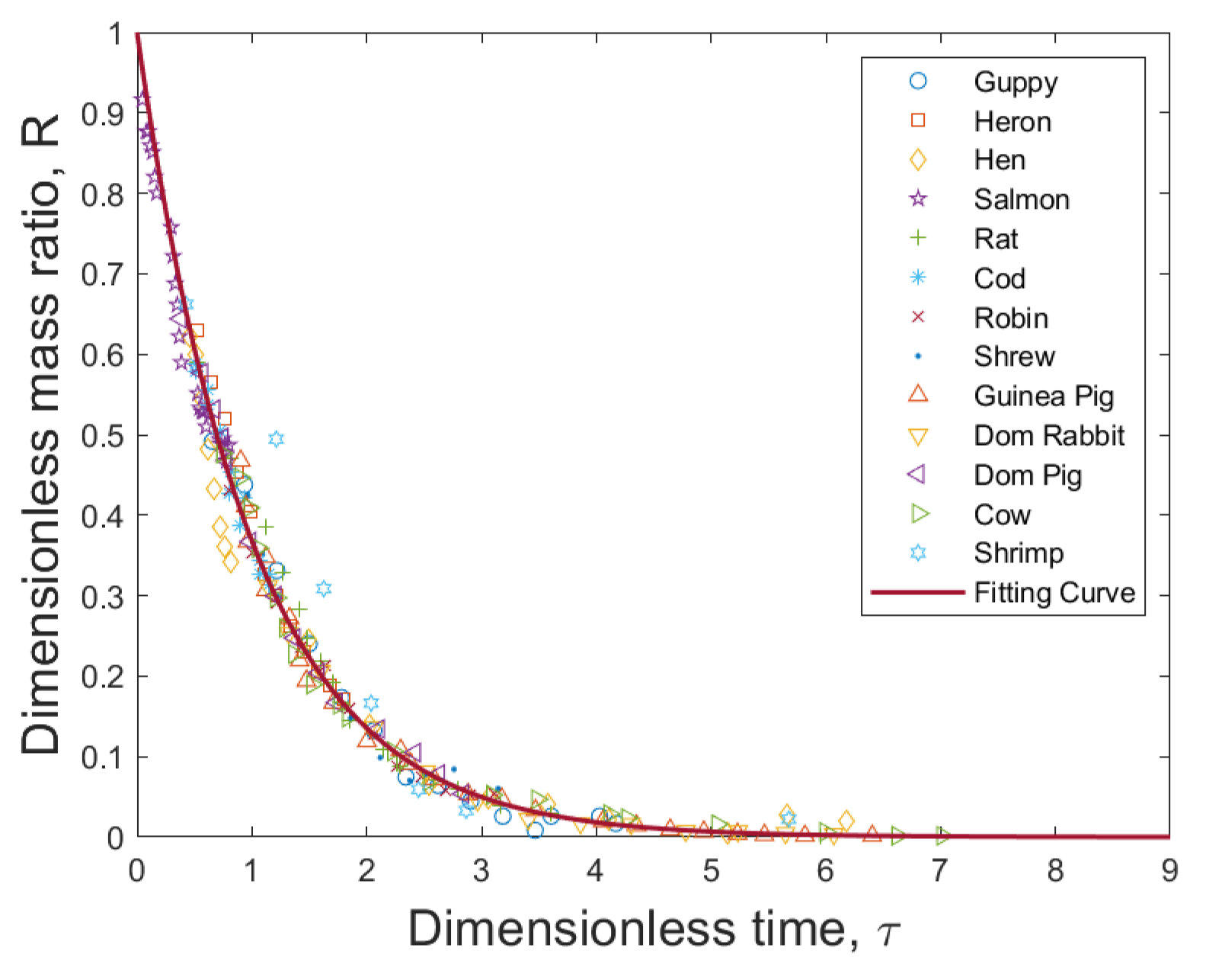
Furthermore, the solution curves suggest some potential frameworks for visualizing data beyond individual species, unveiling universal growth properties across taxonomic groups. In fact, solving equation (5) gives

R (t) = R (0) exp {- \frac{- a t}{4 M^{1 / 4}}}

. If the dimensionless mass ratio R is plotted against a dimensionless time variable

τ = \frac{a t}{4 M^{1 / 4}} - ln (R (0))

, the resulting graph predicts that the body size of all species should adhere to a parameterless universal curve of

R (τ) = e^{- τ}

. The slopes for the growth curves of the 13 animal species closely approximate

- 1

, which implies that growth decelerates as body size increases due to limitations in resource provision by biological networks. Figure 2 shows a plot of the universal deterministic growth curve.

3.4. Diffusion Term Fitting

The patterns of determinate growth species are characterized by a continuous and bounded trajectory. In contrast, the indeterminate growth group exhibits unbounded growth punctuated by intermittent interruptions during the reproduction process. The two groups of growth pattern can be fitted well with the two proposed stochastic models for ontogenetic growth.

Noise intensity

In the following data fitting process, we employ the re-scaled time

τ = - \frac{a}{4 M^{1 / 4}} t

in conjunction with the metabolic distribution

R (τ) = 1 - {(\frac{m (τ)}{M})}^{1 / 4}

. After applying the time-rescaling technique, the stochastic differential equations

()

and

()

are transformed into the following forms.

d R (τ) = - R (τ) d τ + \frac{\bar{σ} R (τ)}{\bar{δ} + R (τ)} d W (τ),

(9)

and

d R (τ) = - R (τ) d τ + \frac{\bar{σ} R (τ) (1 - R (τ))}{\bar{δ} + R (τ)} d W (τ),

(10)

where

\bar{σ}

and

\bar{δ}

are positive constant. The detailed proof of the transformation will be presented later in Section 5.

This transformation involves the conversion of data points from the study by West et al., originally represented as

(t, m (t))

, into an alternative format of

(τ, R (τ))

. Subsequently, we proceed with a comparative analysis, aligning these data points with their corresponding estimated values which are generated from the output of the universal growth curve

R (τ) = e^{- τ}

. We compute the standard deviation

|R_{r e a l} (τ) - R_{e s t i m a t e} (τ)|

, the resulting values are then assigned labels

s_{i}

(

i = 1, 2, . . .

) according to the order of the data samples provided within the dataset.

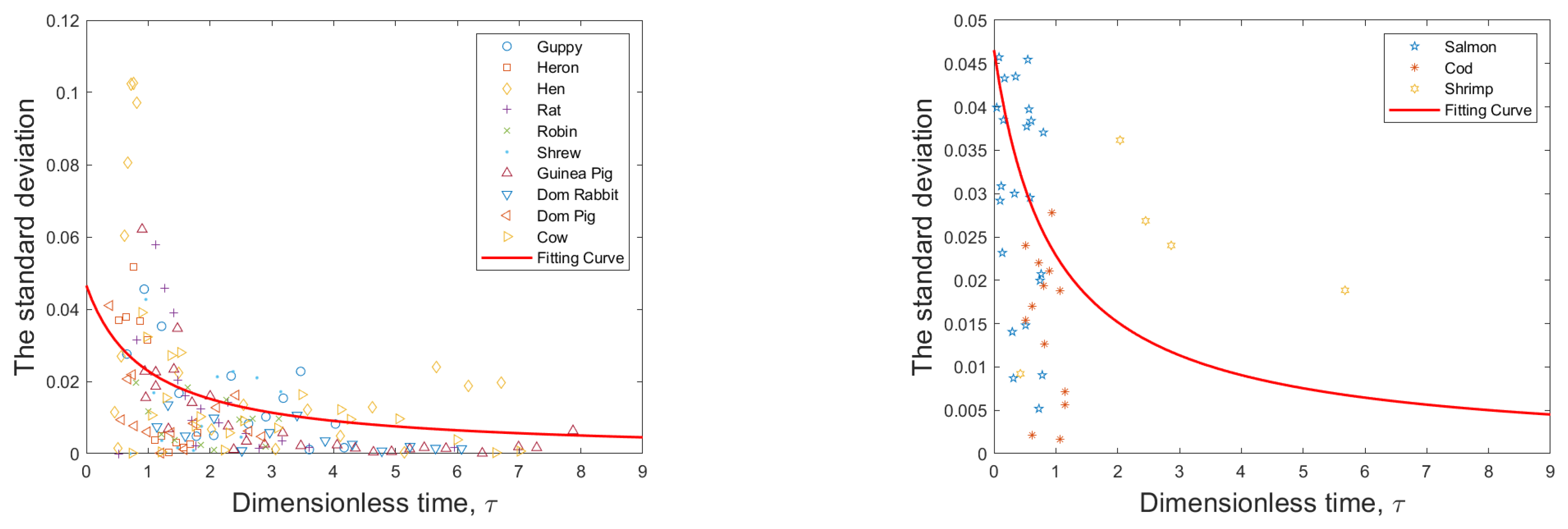
For species with determinate growth patterns, our objective is to ensure that white noise effectively captures the variability within the data set; therefore, we seek to adjust the noise intensity function

g_{1} (R) = \frac{\bar{σ}}{\bar{δ} + R}

to align with the observed standard deviations

(τ, s_{i})

. The optimal fit occurs when

\bar{σ} = 0.045

and

\bar{δ} = 0.9667

, resulting in

R M S E = 0.0215

. For a group of organisms with indeterminate growth patterns, we fit the standard deviations

(τ, s_{i})

to the noise intensity function

g_{2} (R) = \frac{\bar{σ} (1 - R)}{\bar{δ} + R}

. The optimal fit occurs when

\bar{σ} = 0.0181

and

\bar{δ} = 0.2843

, resulting in

R M S E = 0.0426

. Figure 3 shows the fit of the dimensionless standard deviation versus the dimensionless time.

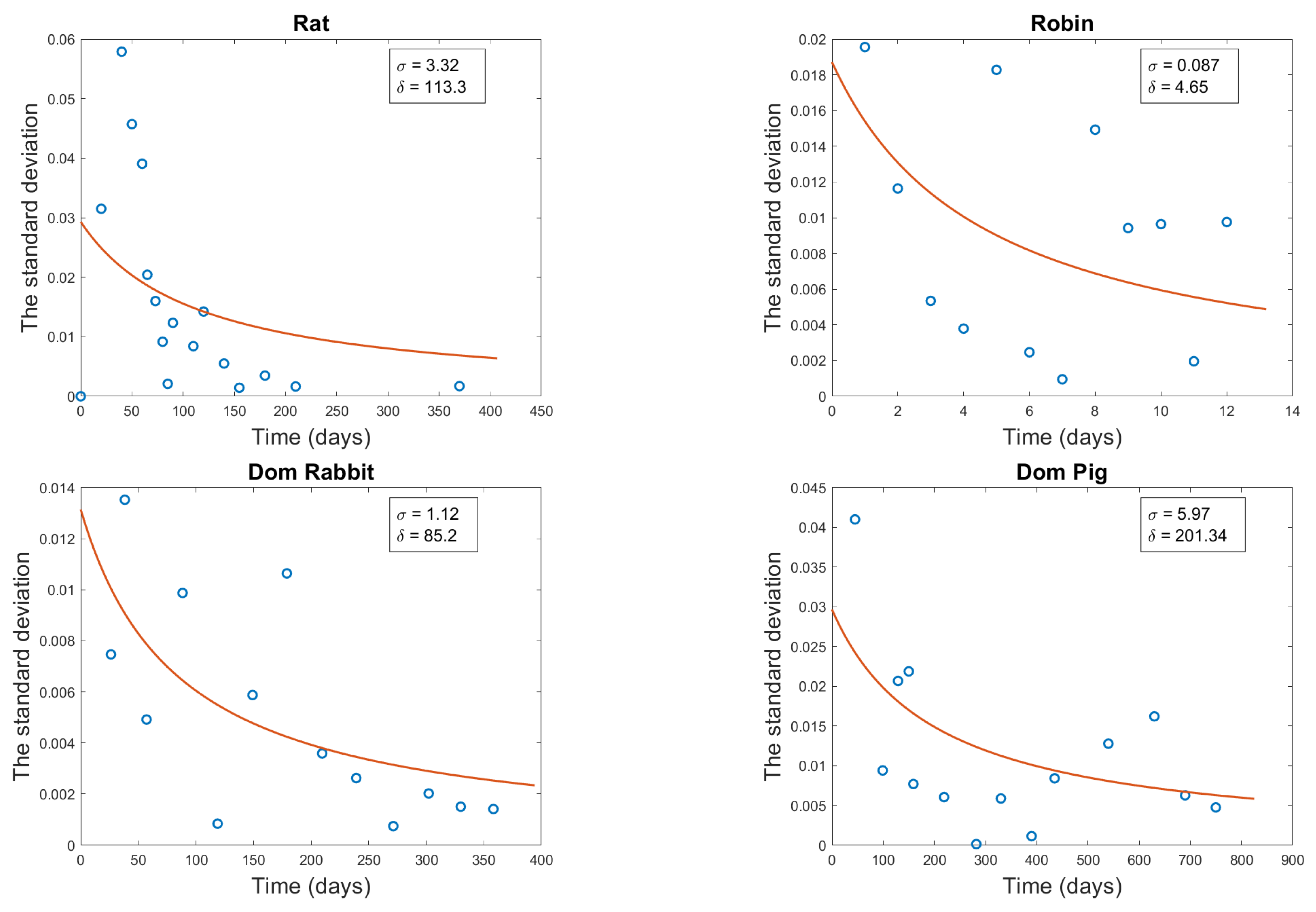
Next, a similar procedure will be performed individually for each animal group to ensure precision. One point to note is that the metabolically distributed

R (t)

is employed but no time rescaling will be carried out; we transform the original data into the format of

(t, R (t))

. We proceed by aligning these real data points with their corresponding estimated value which is generated from the output of the deterministic solution curve

R (t) = R (0) \cdot exp {- \frac{a t}{4 M^{1 / 4}}}

. We compute the standard deviation

|R_{r e a l} (τ) - R_{e s t i m a t e} (τ)|

and present the results as scatter plots. The fitted function

g_{1} (R) = σ / (δ + R)

is used to fit the standard deviations of the determinate group data set. Figure 4 shows four examples of standard deviation fits. These four species are all of the determinate growth type.

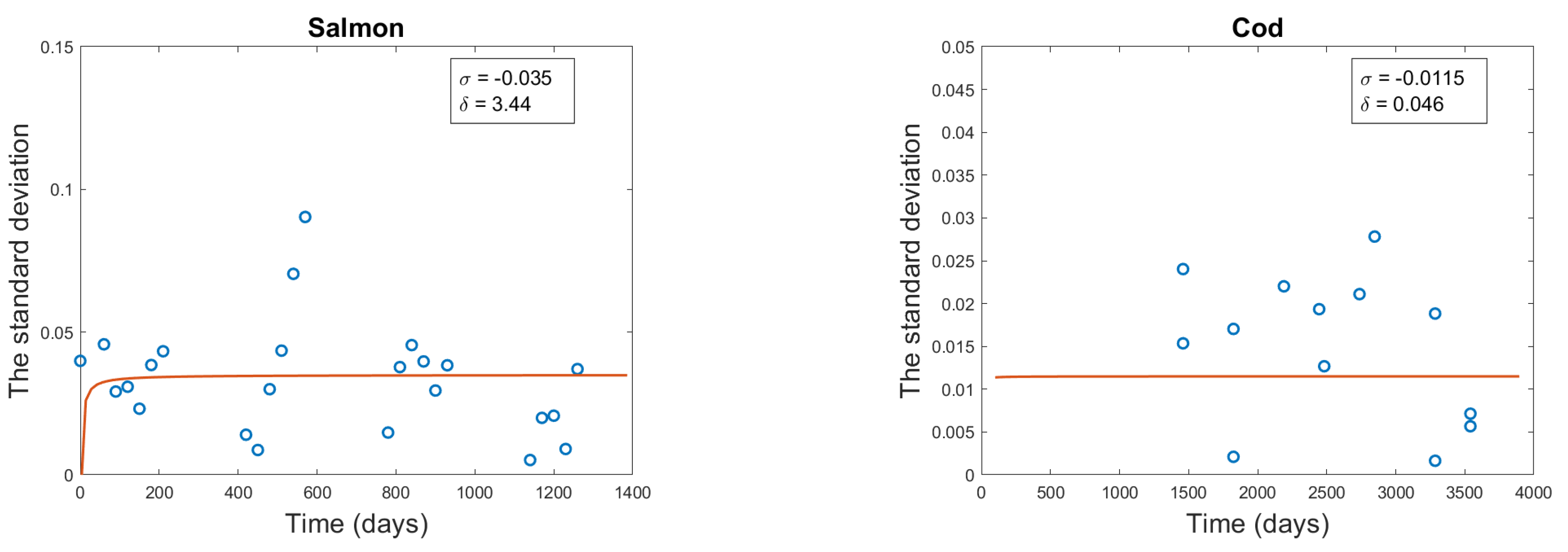
For the indeterminate growth, we take

g_{2} (R) = σ (1 - R) / (δ + R)

to fit the standard deviations for the data set of the indeterminate group. Figure 5 shows two examples of the fitted results.

The optimal fits for the parameters

σ

and

δ

for each species with determinate growth are listed in Table 2.

The optimal fits for the parameters

σ

and

δ

for each species with indeterminate growth are listed in Table 3.

Stochastic solution paths

From the stochastic differential equation (7) for determinate growth, Ito’s formula gives us the solution as follows

R (t) = R (0) exp \{- \frac{a t}{4 M^{1 / 4}} - \int_{0}^{t} \frac{σ^{2}}{2 {(δ + R (s))}^{2}} d s + \int_{0}^{t} \frac{σ}{δ + R (s)} d W (s)\} .

(11)

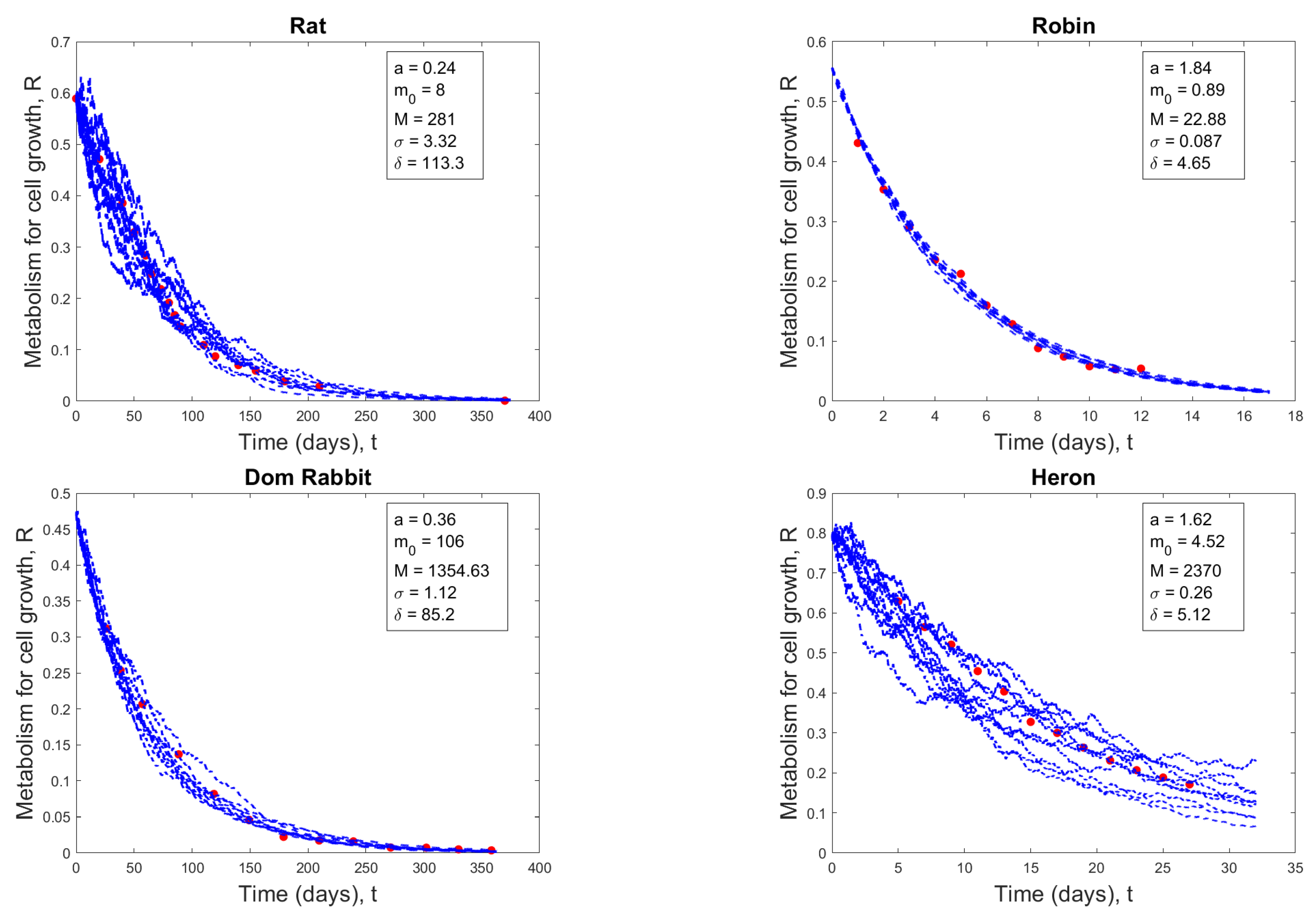
Based on 206 biomass data, we use

R (0)

as an initial condition for SDE and simulate 10 solution sample paths for each species (which makes up to 100 in total). By comparing the data points of each species with the stochastic solution paths corresponding to the set of fitted parameters

(a, m_{0}, M, σ, δ)

, we can see that the above equation (11) captures well the growth pattern of 10 species in the determinate growth. Equation (11) generates a band for each species, with a central curve representing the average biomass and a width indicative of the variance in mass over time.

From these solution sample paths, we obtain an empirical distribution at time t that provides the mean tumor size

μ_{t}

and standard deviation

σ_{t}

. We check if

|R (t) - μ_{t}| \leq 3 σ_{t}

, which gives us a confidence interval of 99%. The results are shown below, which show how the real body sizes will fall in the region of our model prediction if we give a 99% confidence level.

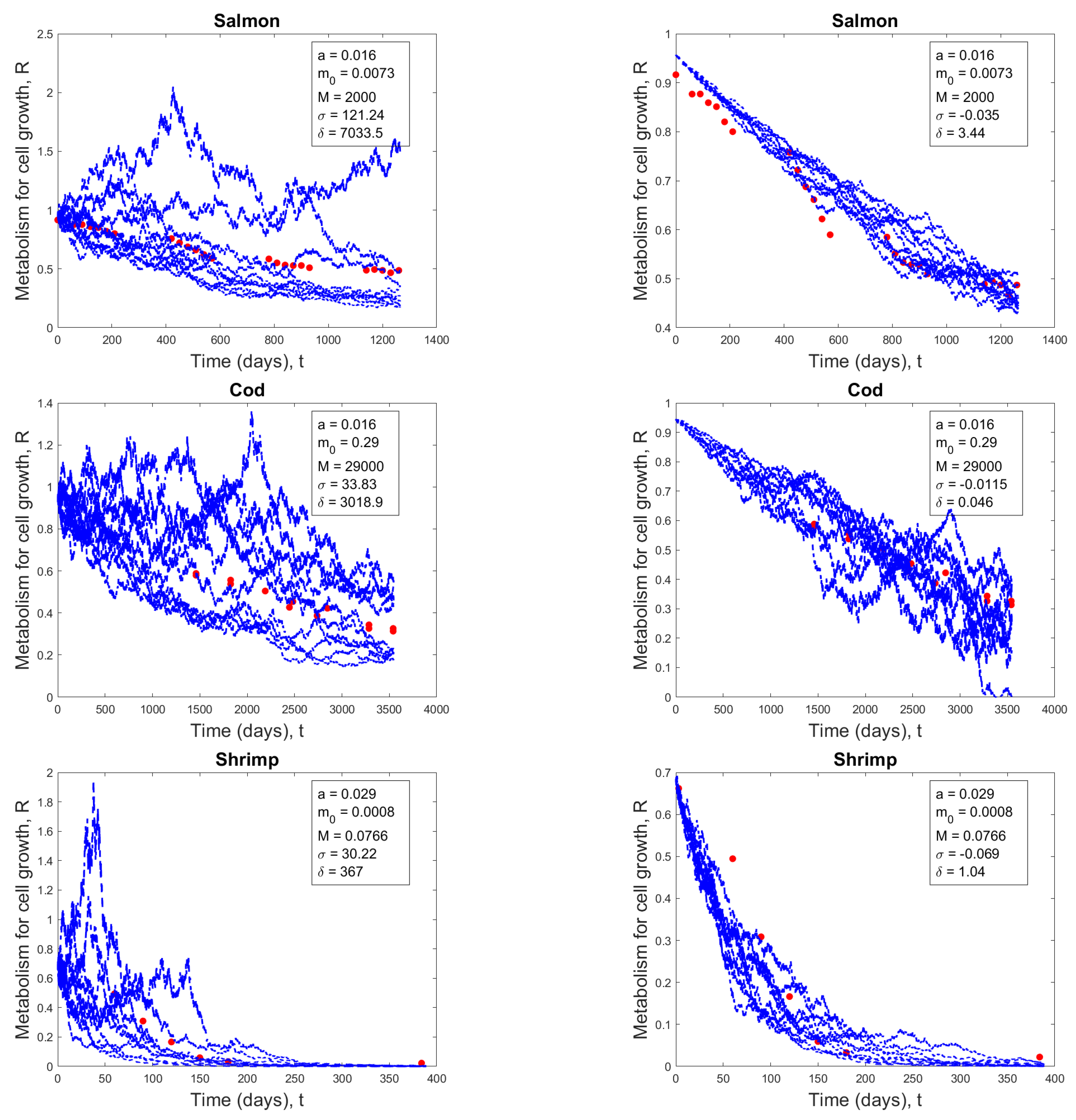
For three species exhibiting indeterminate growth (Salmon, Cod, and Shrimp), when an organism reaches the age for reproduction, a substantial portion of its metabolic energy is allocated to reproduction, resulting in a reduction in the growth rate. We use the stochastic differential equation (8) to catch up on the growth dynamics of these species. To demonstrate the robustness of capturing the noise intensities in the data set of these species using the function

g_{2} (R)

, we use both stochastic differential equations (7) and (8) to fit these data to see which one gives better fitted results. Figure 7 shows the fitted solution paths of (7) and (8) for species in an indeterminate group.

4. Theoretical Analysis

In this section, we will examine the theoretical behaviors of two proposed stochastic differential equations (7) and (8) and explain why these equations are biologically relevant for fitting the data set of 13 species.

Assume that we are working on a complete probability space

(Ω, F, {\{F_{t}\}}_{t \geq 0}, P)

with filtration

{\{F_{t}\}}_{t \geq 0}

satisfying the usual conditions. Since the drift term

- \frac{a R}{4 M^{1 / 4}}

and the two diffusion terms

\frac{σ R}{δ + R}

and

\frac{σ R (1 - R)}{δ + R}

are continuously differential functions and hence locally Lipschitz continuous, there exists a unique locally almost surely continuous solution

R (t)

for both equations (7) and (8). Using standard arguments as in [23], these two equations have unique globally almost surely continuous solutions

R (t)

(0, \infty)

whenever their initial conditions start in

(0, \infty)

. The following two theorems will summarize the dynamical behavior of the solutions of the two equations.

Theorem 1.

For any initial value

R (0) \in (0, \infty)

, there exists a unique almost surely continuous solution

R (t)

to the equation (7) that remains in

(0, \infty)

for all time

t \geq 0

, and

R (t)

is a strong Markov process that satisfies the Feller property. Furthermore, if

R (0) \in (0, \infty)

, then

R (t)

converges exponentially to 0 a.s.

Proof. By applying the Ito’s formula to the equation (7), we obtain

\begin{matrix} R (t) & = R (0) exp \{- \frac{a t}{4 M^{1 / 4}} - \int_{0}^{t} \frac{σ^{2}}{2 {(δ + R (s))}^{2}} d s + \int_{0}^{t} \frac{σ}{δ + R (s)} d W (s)\} \end{matrix}

Because the Brownian Motion

W (t)

can take either negative values or positive values with positive probability, so without loss of generality we can assume that

σ > 0

. Note that all the other parameters are assumed to be positive. Since

R (t) > 0

a.s. for all

t > 0

, the function

\frac{σ}{δ + R (s)}

is bounded and hence, by law of large number, we get

lim_{t \to \infty} \frac{1}{t} \int_{0}^{t} \frac{σ}{δ + R (s)} d W (s) = 0 a . s .

On the other hand,

\frac{1}{t} \int_{0}^{t} \frac{σ^{2}}{2 {(δ + R (s))}^{2}} d s

is always bounded for all time

t > 0

. Therefore,

R (t)

converges exponentially to 0 a.s.

Theorem 2.

For any initial value

R (0) \in (0, 1)

, there exists a unique almost surely continuous solution

R (t)

to the equation (8) that remains in

(0, 1)

for all time

t \geq 0

, and

R (t)

is a strong Markov process that satisfies the Feller property. Furthermore, if

R (0) \in (0, 1)

, then

R (t)

converges exponentially to 0 a.s.

Proof. The argument is totally similar to the proof of Theorem 1. Note that, when

R (0) \in (0, 1)

R (t) \in (0, 1)

a.s. for all times t and hence the function

\frac{σ (1 - R (t))}{δ + R (t)}

is always bounded.

We will end this section with several remarks. First, the two above theorems guarantee that the solutions of both equations (7) and (8) are quickly drawn to the boundary point 0. This is an important property for both equations to fit the data set of 13 species well because if we translate the data set into the form

(t, R (t))

then the data will show a tendency towards zero. Biologically, this makes sense since, over time, each species uses fewer and fewer metabolic energies for its cell growth, and finally this energy decays to 0. Second, the diffusion term

g_{2} (R)

in (8) differs from

g_{1} (R)

in (7) by a factor

1 - R

. We use this factor in

g_{2} (R)

to dampen the function

g_{1} (R)

since the data variation in the indeterminate growth group is much smaller than in the determinate growth group. The other reason is that it makes sure that the solution of equation (8) will live within the interval

(0, 1)

whenever it starts in

(0, 1)

and therefore it will capture the small variations in the indeterminate group.

5. Universal Stochastic Growth Process

Since growth patterns vary between different species that underlie the difference in the parameter set

(a, m_{0}, M, σ, δ)

, our aim is to propose a universal stochastic process that is capable of encapsulating growth patterns between diverse species. To perform this task, we employ the technique of random time change for a stochastic process.

Theorem 3

(Time change formula for Ito integral, see [26]). Suppose

c (s, ω)

and

α (s, ω)

are s-continuous functions such that

α (0, ω) = 0

and

E [α_{t}] < \infty .

Let

B (s)

be an m-dimensional Brownian motion and

v (s, ω)

is bounded, measurable and s-continuous. Define

\tilde{B} (t) = lim_{k \to \infty} \sum_{i}^{k} \sqrt{c (α_{j}, ω)} Δ B (α_{j}) = \int_{0}^{α_{t}} \sqrt{c (s, ω)} d B (s) .

Then

\tilde{B} (t)

is a Brownian motion and martingale with respect to

F_{α_{t}}

and

\int_{0}^{α_{t}} v (s, ω) d B (s) = \int_{0}^{t} v (α_{r}, ω) \sqrt{α^{'} (r, ω)} d \tilde{B} (r)

for almost surely P, where

α^{'} (r, ω)

is derivative of

α (r, ω)

with respect to r and so that

α^{'} (r, ω) = \frac{1}{c (α_{r}, ω)}, for a . a . r \geq 0, ω \in Ω .

First, we apply the theorem to the equation (7). Note that

v (t, ω) = \frac{σ R (t)}{δ + R (t)}

is measurable, bounded and continuous with respect to time t. We consider the inverse-time change

α (t) = τ (t) : = \frac{a t}{4 M^{1 / 4}} .

We can easily check that the time-rescale function is t-continuous, has output of 0 at initial time

t = 0

, and for any fixed t, we have

E [τ (t, R)] = \frac{a t}{4 M^{1 / 4}} < \infty .

Furthermore, by computing the derivative of

α (t)

with respect to time t, it yields the rate of change

c (t) = \frac{4 M^{1 / 4}}{a} .

Therefore, we can define a time-changed Brownian motion

\tilde{W} (t) = \int_{0}^{τ (t)} \sqrt{c (s)} d W (s) = \int_{0}^{τ} \sqrt{\frac{4 M^{1 / 4}}{a}} d W (s) = \sqrt{\frac{4 M^{1 / 4}}{a}} W (τ) .

Then

\int_{0}^{τ} \frac{σ R (s)}{δ + R (s)} d W (s) = \int_{0}^{t} \frac{σ R (τ)}{δ + R (τ)} \sqrt{\frac{a}{4 M^{1 / 4}}} d \tilde{W} (s) = \int_{0}^{t} \frac{σ R (τ)}{δ + R (τ)} d W (τ) .

Under the random time change, the equation (7) becomes a new SDE

d R (τ) = - R (τ) d τ + \frac{σ R (τ)}{δ + R (τ)} \sqrt{\frac{4 M^{1 / 4}}{a}} d W (τ) = - R (τ) d τ + \frac{\bar{σ} R (τ)}{\bar{δ} + R (τ)} d W (τ),

where

\bar{σ} = σ \sqrt{\frac{4 M^{1 / 4}}{a}} and \bar{δ} = δ

. By Ito’s formula, the equation (7) is equivalent to

R (τ) = R (0) exp \{- τ - \int_{0}^{τ} \frac{{\bar{σ}}^{2}}{2 {(\bar{δ} + R (s))}^{2}} d s + \int_{0}^{τ} \frac{\bar{σ}}{\bar{δ} + R (s)} d W (s)\}

With the same inverse-time change

τ (t)

and the same argument as above, the equation (8) is equivalent to

R (τ) = R (0) exp \{- τ - \int_{0}^{τ} \frac{{\bar{σ}}^{2} {(1 - R (s))}^{2}}{2 {(\bar{δ} + R (s))}^{2}} d s + \int_{0}^{τ} \frac{\bar{σ} (1 - R (s))}{\bar{δ} + R (s)} d W (s)\} .

It is challenging to derive a universal stochastic process from these equations after time change. Based on the theoretical result in Section 4, we know that both solutions to these two equations will converge exponentially to 0 a.s. Thus, we propose an estimation as follows. As

R (τ)

approaches 0 and as

τ

is large, we approximate the diffusion terms

\frac{\bar{σ} R (τ)}{\bar{δ} + R (τ)}

of (7) and

\frac{\bar{σ} R (τ) (1 - R (τ))}{\bar{δ} + R (τ)}

of (8) by a single term

\frac{\bar{σ}}{\bar{δ}} R (τ)

. Hence, we propose

d R (τ) = - R (τ) d τ + K R (τ) d W (τ)

(12)

with

K = \bar{σ} / \bar{δ}

. The idea is that with a large data set we can find universal noise that can be applied to all species. With the same mean and slightly larger variance, the equation offers an adequately good stochastic process to capture changes in variation of all species. By Ito’s formula, we can solve for

R (τ) = R (0) exp \{(- 1 - \frac{K^{2}}{2}) τ + K W (τ)\}

(13)

Let

T = τ + \frac{K^{2}}{2} τ

, by performing another time change, equation

()

gives

R (T) = R (0) exp \{- T + \frac{1}{\sqrt{1 + \frac{K^{2}}{2}}} \bar{W} (T)\}

(14)

with

\bar{W} (T)

is a standard Brownian motion. And we can evaluate

\frac{1}{\sqrt{1 + \frac{K^{2}}{2}}} \bar{W} (T)

as a Brownian motion

B (T)

with mean

\frac{1}{1 + \frac{K^{2}}{2}}

to get a universal stochastic process of the form

R (T) = exp \{- T + B (T)\} .

(15)

Given that two of our diffusion models lack closed-form solutions, we cannot obtain exact transition probability distributions for predicting organism sizes. However, we can make numerical predictions for sizes within the prescribed probability bounds. In theory, based on the proposed stochastic differential equations (7) and (8) together with their initial conditions, we can establish a confidence region of a specified probability for an individual’s size at any specific point in the future.

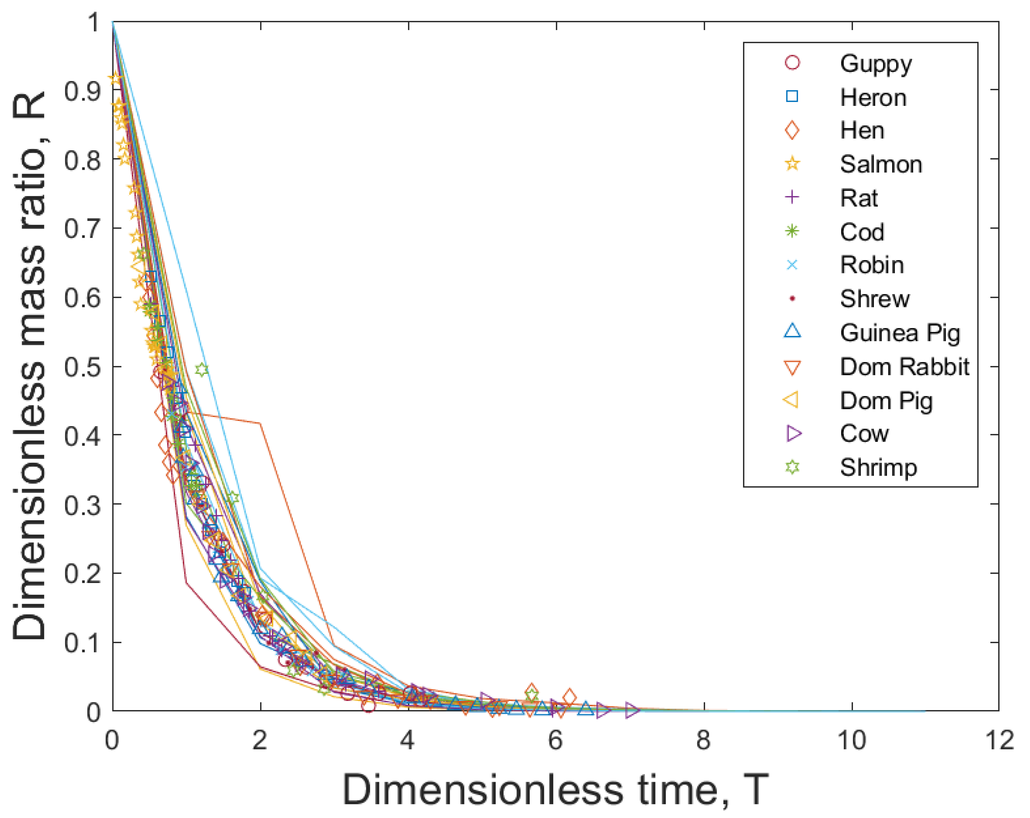
By running data fitting for 13 species for the equation, we have estimated K for each species listed in the following table

()

. Then by taking the mean of the fitted K, we can find a value of K that presents the universal noise for the 13 species. Figure 8 shows the general stochastic band with the fitted parameter

K = - 0.46

6. Discussion

This research was motivated by the broad idea that there should be a general stochastic model for ontogenetic growth if there was a general deterministic model for ontogenetic growth. We carefully studied most of the mathematical models for ontogenetic growth in history [6]. We decided to start with the model proposed by West et al. [11]. Based on the data sets in this study, we attempted to find the best fit for variances of the data under the condition that the fit should have two parameters and a simple mathematical form. It is surprising that this variance fit distinguishes two types of growth, determinate growth, and indeterminate growth. It turns out that we must have two variance fits, one for determinate growth and one for indeterminate growth. We do not achieve a general stochastic model for ontogenetic growth; instead, we obtain a general stochastic model for determinate ontogenetic growth and a general stochastic model for indeterminate ontogenetic growth if we could claim this, as West et al. did. However, we still can ask with what new variance form can we obtain a general stochastic model for ontogenetic growth based on the data sets in the study of West et al. This is an interesting question, and we will consider it in the future.

Based on their general model for ontogenetic growth, West et al. produced a universal growth curve. It is well known that, in the deterministic case, it is easy to obtain a universal solution curve after an appropriate time change. We plot such a universal growth curve as the dimensionless mass ratio R against dimensionless time. For two stochastic models for ontogenetic growth we obtained, we expect to get two universal stochastic growth curves, one for determinate growth and one for indeterminate growth. However, it was difficult to perform the stochastic time change without explicit solution forms. We may achieve them by numerical study. But, we made some approximation of noise terms and stochastic transformation of time, we then obtained an approximation of universal stochastic curve which is a geometric Brownian motion multiplied by an exponential time factor. The universal (deterministic and stochastic) growth curve should be a general phenomenon no matter what scaling exponent is used in modeling.

There were many studies about scaling law in ontogenetic growth. The researchers choose the scaling exponent

\frac{3}{4}

\frac{2}{3}

for energy acquisition with respect to mass, then perform data analysis to fit their models. Some research left the scaling exponent as an unknown and tried to estimate it from their data. It seems that a general study of the Bertalanffy-type ontogenetic growth equation is needed. For this, we may consider both metabolic power for maintenance and growth to be some scalings with respect to mass

\frac{d m}{d t} = a m^{α} - b m^{β}

. In the classical work [6], it has already proposed such a general mathematical model. This general equation may provide more freedom to build a general stochastic model for ontogenetic growth. This is an interesting idea that is worth exploring further.

It may be interesting to study the ontogenetic growth of a cell, starting from the birth of a new cell until cell division. This will require details of cell biology and related data. The precise mathematical model may be established for a cell.

Tumor growth modeling has been a significant research area that provides not only new theoretic mathematical problems but also, more importantly, insight and treatment suggestions for cancer researchers. There are several methods to construct mathematical models for tumor growth, for example, mass conservation law, fluid dynamics. Energy allometry is a new way to build tumor growth models. Some studies have applied energy allometric theory to tumor growth [24,25]. Energy allometry may provide new insight into the field.

Acknowledgments

TAP would like to thank the support of the National Institute of General Medical Sciences of the National Institutes of Health under Award Number P20GM104420.

References

Carrel, A. (1931) Physiological time. Science 74, 618.
Brody, S. (1945) Bioenergetics and Growth. Hafner, New York.
von Bertalanffy, L. (1938) A quantitative theory of organic growth. Human Biology 10, 181–213.
von Bertalanffy, L. (1957) Quantitative laws in metabolism and growth. Quarterly Review of Biology 32, 217–231.
Sibly, R.M. & Calow, P. (1987) Growth and resource allocation. Evolutionary Physiological Ecology, pp. 37–52. Cambridge University Press, Cambridge.
Reiss, M.J. (1989) The allometry of growth and reproduction.
Kooijman, S.A.L.M. (1993) Dynamic Energy Budgets in Biology Systems. Theory and Applications in Ecotoxicology. Cambridge University Press, Cambridge.
Ricklefs, R.E. (1967) A graphical method of fitting equations to growth curves. Ecology 48, 978–983.
Ricklefs, R.E. (2003) Is rate of ontogenetic growth constrained by resource supply or tissue growth potential? A comment on West et al. 17.
Case, T.J. (1978) On the evolution and adaptive significance of postnatal growth rates in the terrestrial vertebrates. Quarterly Review of Biology 29, 103–137.
Geoffrey, B. West, James H. Brown & Brian J. Enquist, A general model for ontogenetic growth, Nature volume 413, pages628–631 (2001).
West, G.B. , Brown, J. J. ( 1997) A general model for the origin of allometric scaling laws in biology. Science 276, 122–126.
West, G.B. , Enquist, B.J. & Brown, J.H. (2002) Modelling universality and scaling: reply. Nature 420, 626–627.
Makarieva A.M., V. G. Gorshkov, B.-L. Li, Ontogenetic growth: models and theory, Ecological Modelling 176 (2004) 15–26.
Moses M.E., C. Hou, W.H. Woodruff, G.B. West, J.C. Nekola, W. Zuo, and J.H. Brown, Revisiting a model of ontogenetic growth: estimating model parameters from theory and data, the American Naturalist, 2008. Vol. 171, (3) 632–645.
Hou, C. , Bolt K. R. Soc. B ( 2011) 278, 2881–2890.
Shi P-J., X-Y Men, H.S. Sandhu, A Chakraborty, B-L Li, F Ou-Yang, Y-C Sun, F Ge, The “general”ontogenetic growth model is inapplicable to crop growth, Ecological Modelling 266 (2013) 1– 9.
Sibly, R. M, J. Baker, J.M. Grady, S.M. Luna, A. Kodric-Brownb, C. Venditti, and J.H. Brown, Fundamental insights into ontogenetic growth from theory and fish, PNAS, 2015, Vol. 112, (45) 13934-13939.
Hatton I.A., A. P. Dobson, D. Storch, E.D. Galbraithe, and M. Loreau, Linking scaling laws across eukaryotes, PNAS, 2019, 116(43):21616–21622.
Escala A, Universal ontogenetic growth without fitted parameters: implications for life history invariants and population growth, Theoretical Ecology (2023) 16:315–325.
West, B.J. , and D. West, Stochastic ontogenetic growth model, A Letter Journal Exploring the Frontiers of Physics, 2012, 97, 48002. [Google Scholar]
Ziwei Ma, Ben Niu, Tuan Anh Phan, Anne Line Stensjoen, Chibawanye Ene, Timothy Woodiwiss, Tonghui Wang, Philip K. Maini, Eric C. Holland & Jianjun Paul Tian, Stochastic growth pattern of untreated human glioblastomas predicts the survival time for patients, Scientific Reports, Volume 10, Article number: 6642 (2020).
Phan, T.A.; Wang, S.; Tian, J.P. Analysis of a new stochastic Gompertz diffusion model for untreated human glioblastomas. Stochastics Dyn. 2022, 2250019. [Google Scholar] [CrossRef]
Guiot, C., P. G. Degiorgis, P.P. Delsanto, P. Gabriele, T.S. Deisboeck, 2003. Does tumor growth follow a “universal law”? J. Theor. Biol. 225, 147–151.
2024; 86.
Bernt Oksendal, An introduction to stochastic differential equations with applications, 5th edition, Springer-Verlag Heidelberg New York.

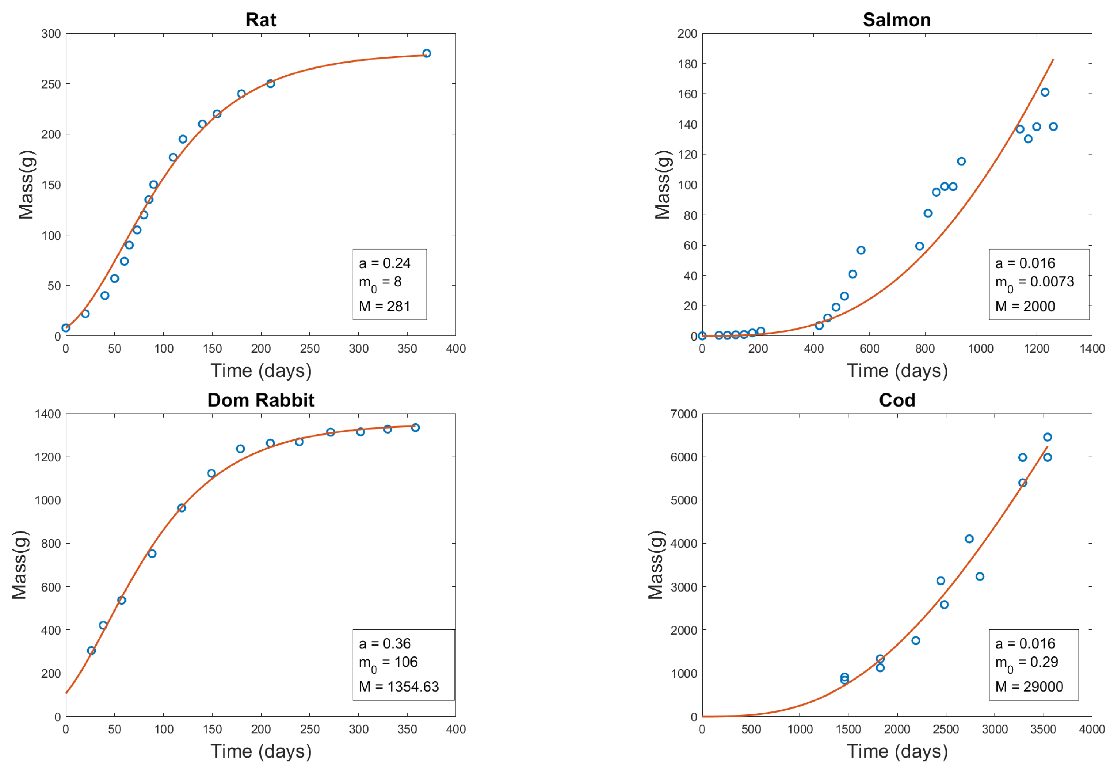
Figure 1. Four examples of fits to growth curves (solid line): left panel are determinate growth, right panel are indeterminate growth.

Figure 2. Universal Deterministic Growth Curve. A plot of the dimensionless mass ratio R, versus the dimensionless time variable

τ

for all 13 organisms (shown as a solid line).

Figure 2. Universal Deterministic Growth Curve. A plot of the dimensionless mass ratio R, versus the dimensionless time variable

τ

for all 13 organisms (shown as a solid line).

Figure 3. Plots of the dimensionless standard deviation s, versus the dimensionless time variable

τ

for determinate and indeterminate groups fits to the corresponding noise intensity functions

g_{1} (R)

and

g_{2} (R)

Figure 3. Plots of the dimensionless standard deviation s, versus the dimensionless time variable

τ

for determinate and indeterminate groups fits to the corresponding noise intensity functions

g_{1} (R)

and

g_{2} (R)

Figure 4. Four determinate growth examples of fitting standard deviations to the curve

g_{1} (R)

(solid lines).

Figure 4. Four determinate growth examples of fitting standard deviations to the curve

g_{1} (R)

(solid lines).

Figure 5. Two indeterminate growth examples of fitting standard deviations to the curve

g_{2} (R)

(solid lines).

Figure 5. Two indeterminate growth examples of fitting standard deviations to the curve

g_{2} (R)

(solid lines).

Figure 6. Four examples of comparing data points (red dots) with solution paths (11) (blue curves) of determinate growth.

Figure 7. Solution paths are generated by (7) (left panel) and (8) (right panel) when they are fitted to indeterminate growth data sets.

Figure 8. Universal Stochastic Growth Process. A plot of the dimensionless mass ratio R versus the dimensionless time variable T for all organisms falls in the band of the stochastic solution paths (15) with fitted parameters (solid lines).

Table 1. Values of estimated parameters a,

m_{0}

, and M for 13 organisms.

Table 1. Values of estimated parameters a,

m_{0}

, and M for 13 organisms.

Organism	a	$m_{0}$ (g)	M (g)
Guppy	0.1	0.008	0.15
Heron	1.62	4.52	2,370
Hen	0.47	38	2,100
Rat	0.24	8	281
Robin	1.84	0.89	22.88
Shrew	0.75	0.3	4.55
Guinea Pig	0.21	1.78	830.15
Domestic Rabbit	0.36	106	1,354.63
Domestic Pig	0.33	482	311,800
Cow	0.27	33,300	444,490
Salmon	0.016	0.0073	2,000
Cod	0.016	0.29	29,000
Shrimp	0.029	0.0008	0.0766

Table 2. Values of estimated parameters

δ

and

σ

for species with determinate growth.

Table 2. Values of estimated parameters

δ

and

σ

for species with determinate growth.

Organism	$σ$	$δ$	RMSE
Guppy	0.93	24.87	0.0098
Heron	0.26	5.12	0.0132
Hen	5.54	96.19	0.0315
Rat	3.32	113.3	0.0162
Robin	0.087	4.65	0.0061
Shrew	4.28	313.34	0.0133
Guinea Pig	1.11	40.6	0.0083
Domestic Rabbit	1.12	85.2	0.0033
Domestic Pig	5.97	401.34	0.0066
Cow	15.53	778.43	0.0102

Table 3. Values of estimated parameters

δ

and

σ

for species with indeterminate growth.

Table 3. Values of estimated parameters

δ

and

σ

for species with indeterminate growth.

Organism	$σ$	$δ$	RMSE
Cod	-0.0115	0.046	0.0087
Salmon	-0.035	3.44	0.00218
Shrimp	-0.069	1.04	0.0726

Table 4. Values of

\bar{σ}

\bar{δ}

and corresponding K for different species.

Table 4. Values of

\bar{σ}

\bar{δ}

and corresponding K for different species.

Organism	$\bar{σ}$	$\bar{δ}$	K
Guppy	4.64	24.87	0.1866
Heron	1.08	5.12	0.2108
Hen	42.05	96.19	0.4372
Rat	27.43	113.3	0.2421
Robin	0.19	4.65	0.0408
Shrew	11.95	313.34	0.0381
Guinea Pig	11.22	40.6	0.2764
Domestic Rabbit	9.2	85.2	0.1079
Domestic Pig	101.04	401.34	0.2517
Cow	303.74	778.43	0.3902
Cod	-0.66	0.092	-7.1397
Salmon	-1.43	3.44	-0.416
Shrimp	-0.59	1.04	-0.5652

Disclaimer/Publisher’s Note: The statements, opinions and data contained in all publications are solely those of the individual author(s) and contributor(s) and not of MDPI and/or the editor(s). MDPI and/or the editor(s) disclaim responsibility for any injury to people or property resulting from any ideas, methods, instructions or products referred to in the content.

© 2024 by the authors. Licensee MDPI, Basel, Switzerland. This article is an open access article distributed under the terms and conditions of the Creative Commons Attribution (CC BY) license (http://creativecommons.org/licenses/by/4.0/).

Copyright: This open access article is published under a Creative Commons CC BY 4.0 license, which permit the free download, distribution, and reuse, provided that the author and preprint are cited in any reuse.

MDPI Initiatives

Important Links

Choose an area of interest and we will send you notifications of new preprints at your preferred frequency.

Disclaimer

Stochastic Models for Ontogenetic Growth

Abstract

1. Introduction

2. Mathematical Model Setup

2.1. General Deterministic Model for Ontogenetic Growth

2.2. Stochastic Models for Ontogenetic Growth

3. Parameter Fitting

3.1. Dataset

3.2. Fitting Method

3.3. Drift Term Fitting

3.4. Diffusion Term Fitting

Noise intensity

Stochastic solution paths

4. Theoretical Analysis

5. Universal Stochastic Growth Process

6. Discussion

Acknowledgments

References

MDPI Initiatives

Important Links

Subscribe