Submitted:
15 October 2024
Posted:
17 October 2024
You are already at the latest version
Abstract
Keywords:
1. Introduction
2. Multi-Arm Mach-Zehnder Interferometer
3. Fiber optic MAMZI
4. MAMZI with Phase Noise Stabilization
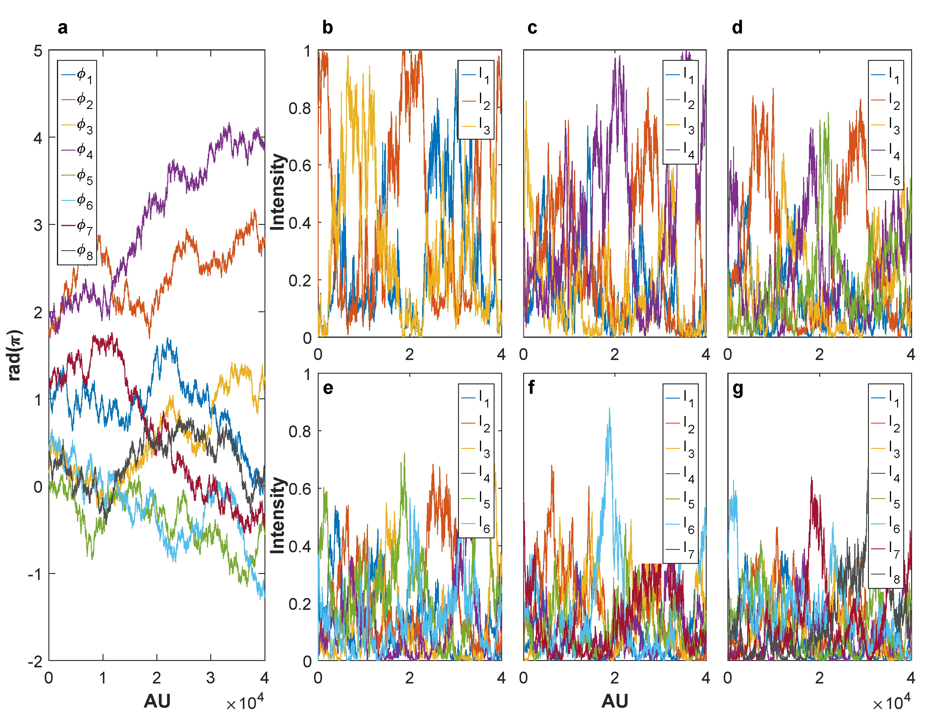
4.1. MAMZI Simulation with Phase Noise
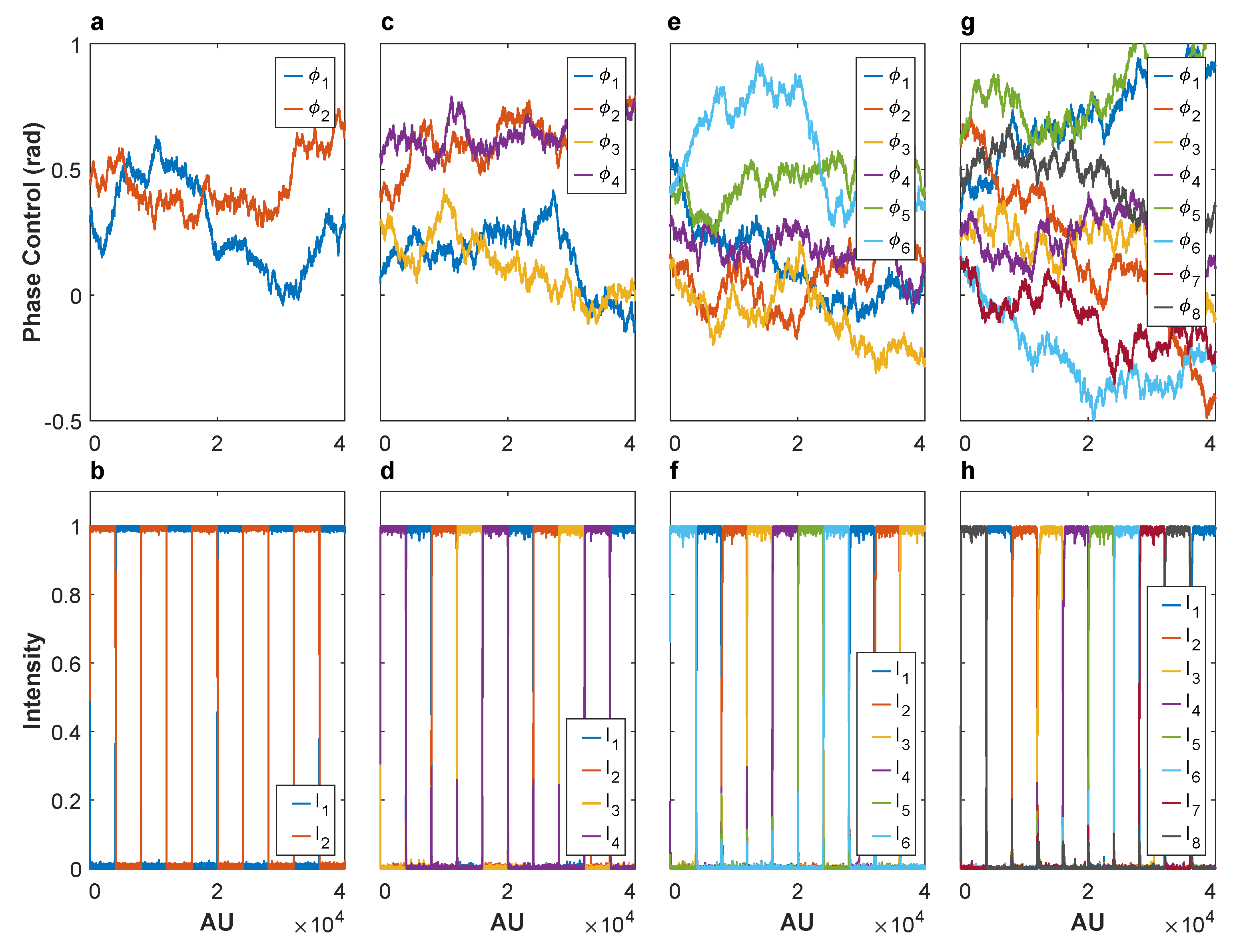
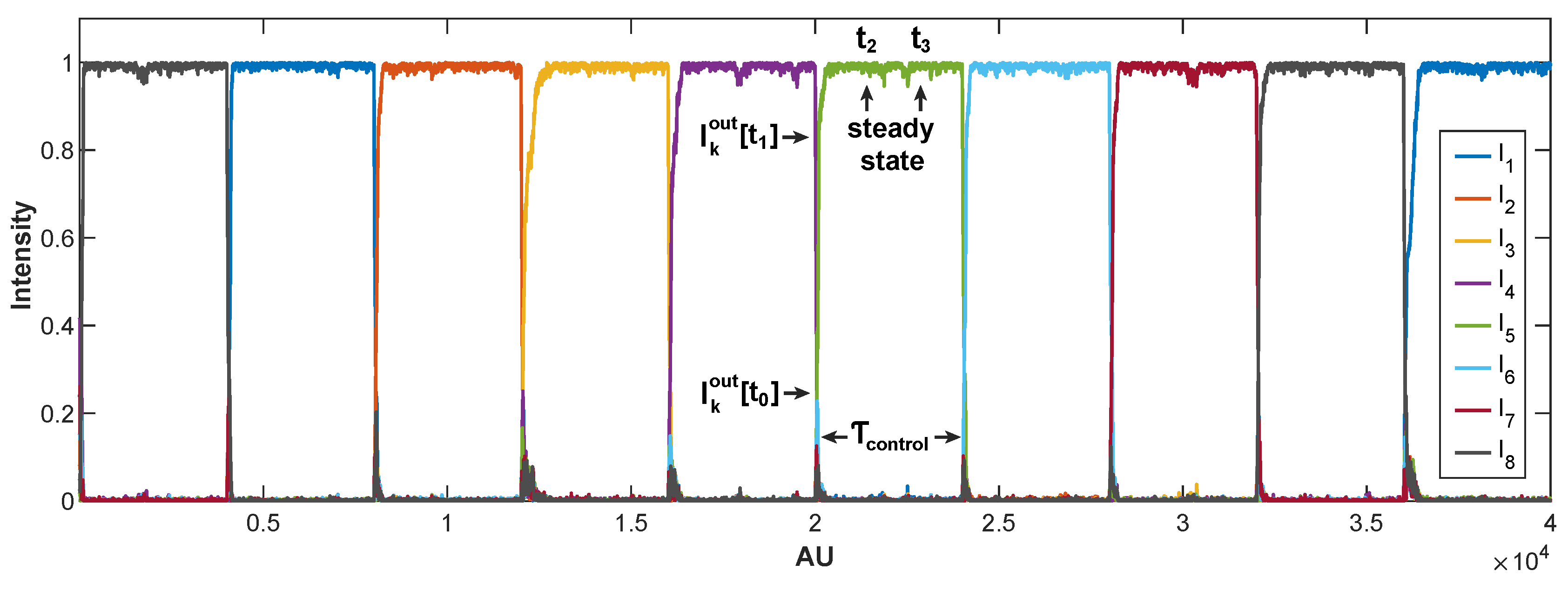
4.2. Operation of the Control Algorithm
- (i)
- The algorithm evaluates the error defined as , where is the measured intensity at output and is a reference value. If the error exceeds a predefined threshold (usually less than 0.001 to reach high visibility [22]), the optimization process starts in the initial work cycle ("").
- (ii)
- As the amplitude of random phase noise in this simulation is , the equation perturbs the phase control as: , where the step is a manually adjustable value. The sign of the disturbance depends on the variation of , indicating whether it increases or decreases, reaching a local maximum for output in its phase space.
- (iii)
- The algorithm then proceeds to perturb the next phase ("") of the other arm of the MAMZI, repeating step (ii).
- (iv)
- Once all phases have been processed, the system restarts the cycle from step (i), continuing the iterative optimization process.
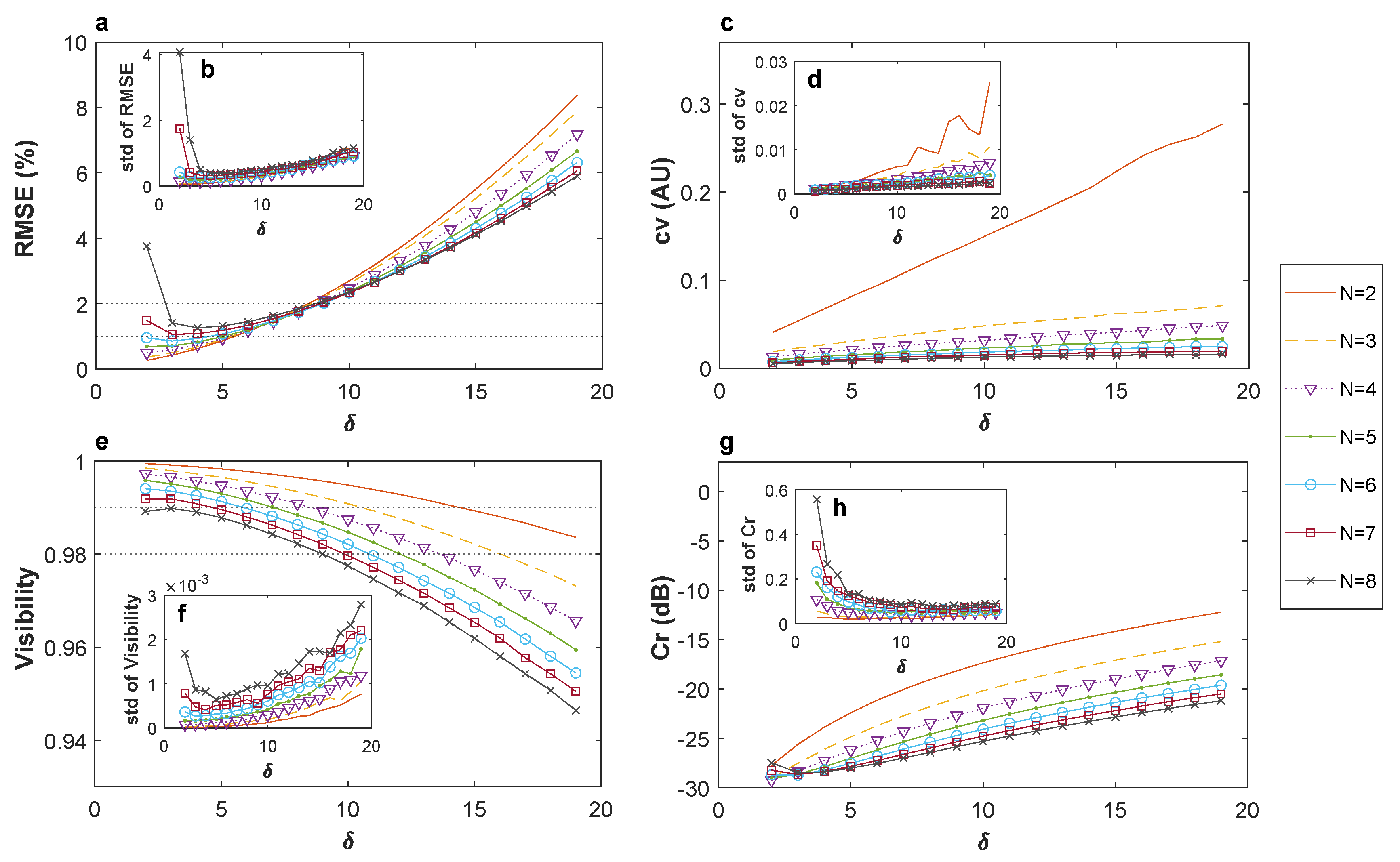
4.3. Analysis of the Results in Phase Noise Stabilization
5. Conclusions
Author Contributions
Acknowledgments
References
- Elsherif, M.,Salih, A.E., Muñoz, M.G., et al, Optical Fiber Sensors:Working Principle, Applications, and Limitations. Adv. PhotonicsRes., 3, 2699-9293(2022).
- Lecheng Li, Li Xia, Zhenhai Xie, and Deming Liu, "All-fiber Mach-Zehnder interferometers for sensing applications," Opt. Express.20, 11109-11120 (2012).
- Tetsuya K, Takahide S, Tetsuya M, et al, "High-speed optical DQPSK and FSK modulation using integrated Mach-Zehnder interferometers," Opt. Express 14, 4469-4478 (2006).
- N. Gisin, G. Ribordy, W. Tittel, and H. Zbinden, "Quantum Cryptography", Rev. Mod. Phys. 74, 145 (2002).
- A. Cuevas, G. Carvacho, G. Saavedra, et al.,"Long-distance distribution of genuine energy-time entanglement," Nat. Commun 4, 2871 (2013).
- F. Vedovato, C. Agnesi, M. Tomasin, M. Avesani, L. Jan-Åke, G. Vallone, and P. Villoresi, "Postselection-Loophole-Free Bell Violation with Genuine Time-Bin Entanglement", Phys. Rev. Lett. 121, 190401 (2018).
- D. Grassani, M. Galli, D. Bajoni, "Active stabilization of a Michelson interferometer at an arbitrary phase with subnanometer resolution", Opt. Lett., 39, 2530-2533 (2014).
- G. B. Xavier and J. P. V. der Weid, "Stable single-photon interference in a 1 km fiber-optic Mach–Zehnder interferometer with continuous phase adjustment", Opt. Lett. 36, 1764 (2011).
- G Carvacho, J. Cariñe, G. Saavedra, et al., "Postselection-Loophole-Free Bell Test Over an Installed Optical Fiber Network", Phys. Rev. Lett. 115, 030503 – Published 14 July 2015.
- V. Giovannetti, S. Lloyd, and L. Maccone, "Quantum-enhanced measurements: beating the standard quantum limit", Science, 306, 1330-1336, 2004.
- M. A. Nielsen and I. L. Chuang, "Quantum Computation and Quantum Information: 10th Anniversary Edition"., Cambridge: Cambridge University Press. 2010.
- B. P. Lanyon et al., "Simplifying quantum logic using higher-dimensional Hilbert spaces", Nature Physics, 5, pp. 134-140, 2009.
- N. J. Cerf, M. Bourennane, A. Karlsson, and N. Gisin, "Security of quantum key distribution using d-level systems", Phys. Rev. Lett. 88, 127902 (2002).
- V. Scarani et al., "The security of practical quantum key distribution", Reviews of Modern Physics, 81, pp. 1301-1350, 2009.
- G. Cañas, N. Vera, J. Cariñe, et al., "High-dimensional decoy-state quantum key distribution over multicore telecommunication fibers", Phys. Rev. A 96, 022317 (2017).
- Ding, Y., Bacco, D., Dalgaard, K. et al. High-dimensional quantum key distribution based on multicore fiber using silicon photonic integrated circuits. npj Quantum Inf, 3, 25 (2017).
- Lee, H.J., Choi, SK. and Park, H.S. Experimental Demonstration of Four-Dimensional Photonic Spatial Entanglement between Multi-core Optical Fibres. Sci Rep, 7, 4302 (2017).
- E.S. Gómez, S. Gómez, I. Machuca, et al., "Multidimensional Entanglement Generation with Multicore Optical Fibers", Phys. Rev. Applied, 15, 034024, (2021).
- L. Gan, R. Wang, D. Liu, L. Duan, S. Liu, S. Fu, B. Li, Z. Feng, H. Wei, W. Tong, et al., "Spatial-division multiplexed Mach–Zehnder interferometers in heterogeneous multicore fiber for multidimensional measurement", IEEE Photonics J. 8, 7800908 (2016).
- D. Balado, J. Liñares, X. Prieto-Blanco, and D. Barral, "Phase and polarization autocompensating N-dimensional quantum cryptography in multicore optical fibers," J. Opt. Soc. Am. B, 36, 2793-2803 (2019).
- Da Lio, B., Cozzolino, D., Biagi, N. et al. Path-encoded high-dimensional quantum communication over a 2-km multicore fiber. npj Quantum Inf,7, 63 (2021).
- J. Cariñe, G. Cañas, P. Skrzypczyk, et al., "Multi-core fiber integrated multi-port beam splitters for quantum information processing", Optica,7, 542-550, 2020.
- M.M. Taddei, J. Cariñe, D. Martínez, et al., "Computational advantage from the quantum superposition of multiple temporal orders of photonic gates", PRX Quantum,2,010320, (2021).
- Yatinkumar, P. "A Comprehensive Review of Maximum Power Point Tracking Techniques for Photovoltaic Systems". Renewable and Sustainable Energy Reviews, 112, 379-387. (2020). 2020.
- M. A. Elgendy, B. Zahawi and D. J. Atkinson, "Assessment of Perturb and Observe MPPT Algorithm Implementation Techniques for PV Pumping Applications," IEEE Transactions on Sustainable Energy,3, 21-33, (2012).
- T. Esram and P. L. Chapman, "Comparison of Photovoltaic Array Maximum Power Point Tracking Techniques," in IEEE Transactions on Energy Conversion, 22, 439-449,(2007).
- Y. Ji, B. Wu, Y. Hou and A. Ding, "A MZ Modulator Bias Control System Based on Variable Step P&O Algorithm", IEEE Photonics Technology Letters, 32, 1473-1476,(2020).
- K Mattle, M Michler, H Weinfurter, A Zeilinger, M Zukowski, "Nonclassical statistics at multiport beam-splitters", Applied Physics B-Lasers and Optics, 60, 111-117, (1995).
- G.Weihs, M. Reck, H.Weinfurter, and A. Zeilinger, “All-fiber three-path mach-zehnder interferometer," Opt. Lett., 21, 302-304, (1996).
- Thorlabs, Inc. Available at: https://www.thorlabs.com/ (Accessed: 01 October 2024).
- Preumont, A. "Controllability and Observability", Vibration Control of Active Structures. Solid Mechanics and Its Applications, 179, 275-297. Springer, (2011).


Disclaimer/Publisher’s Note: The statements, opinions and data contained in all publications are solely those of the individual author(s) and contributor(s) and not of MDPI and/or the editor(s). MDPI and/or the editor(s) disclaim responsibility for any injury to people or property resulting from any ideas, methods, instructions or products referred to in the content. |
© 2024 by the authors. Licensee MDPI, Basel, Switzerland. This article is an open access article distributed under the terms and conditions of the Creative Commons Attribution (CC BY) license (http://creativecommons.org/licenses/by/4.0/).


