1. Introduction
Recent advances in robotics technology have demonstrated that robots are capable of assisting people or even labor in certain tasks that are repetitive and physically demanding for human workers such as material handling, assembly, quality control in manufacturing settings [
1] or picking and transporting fruit in agricultural applications [
2]. Autonomous mobile robots often face issues from external or uncontrollable factors, including unexpected dynamic obstacles and variations in uneven terrain layout, which is typical in outdoor applications such as agriculture and forestry. Indeed, if one focuses on outdoor applications, navigating uneven terrain conditions usually represents challenges such as dealing with slopes, declines, structural rigidness, flexibility, and other terrain characteristics. The slippage phenomenon may occur in such situations, which can lead to trajectory tracking errors and potential robot damage when the system works in confined spaces. However, previous motion controllers have not accounted for the navigation terrain, which could be considered as the primary terra-mechanical constraint that may impact on the control performance of the autonomous ground vehicles through reduced tractive force exertion and wheel slippage [
3].
A robotic arm mechanically attached to a mobile base is often referred to as a mobile manipulator [
4]. This coupling stands for interactions between forces generated by object manipulation, the manipulator-base joint and the wheel-terrain contact. These interactions usually result in bidirectional disturbances in the robotic system. In addition to maneuverability, obstruction with dynamic obstacles appearing unexpectedly around mobile robots, tractive force losses caused by low-friction terrain or noncontact conditions become a critical disturbance source as they lead to performance degradation and, consequently, to the potential risk of slippage or wheel entrapment. Formulating a motion model of the mobile manipulator dynamics under ideal conditions without slip could yield not enough motion accuracy [
5]. In the analyses of autonomous mobile robots and motion controllers, some authors assume the fulfillment of nonholonomic constraints [
6,
7,
8], which could lead mobile robots to navigate without experiencing slippage [
9]. However, wheel slippage occurs frequently in real-world scenarios, particularly on low-friction surfaces, uneven terrain, or in relative high-speed maneuvers. The slip conditions could be considered as model uncertainties within its formulation as they are not often known and accounted for motion models of the vehicle dynamics. Thus, it is required to investigate mobile robot control approaches that integrate aspects related to wheel slip, modeling errors, and external disturbances.
Combined control strategies for manipulation systems that integrate the dynamics of both the mobile base and robotic arm have been extensively studied in the literature [
7,
10,
11,
12]. However, further research is needed to address disturbance rejection in tire-terrain interactions and the resulting propagation of these disturbances through motion coordination to the robot’s arms and joints. Traditional techniques such as PID, backstepping, and adaptive control have been widely investigated to coordinate mobile manipulators and mitigate uncertain dynamics caused by the wheel slip and nonholonomic constraints [
7]. For instance, works on feedback linearization or Lyapunov techniques with parametrized robot models can be found in [
13]. However, they are limited to search of applicable Lyapunov functions or nonlinear simplifications of the robot model. The application of these techniques inevitably results in the loss of the system fidelity from the original system. Classical control approaches and algorithms such as fuzzy logic-based or neural network control [
14,
15,
16,
17], can restrict model fidelity, specially in terra-mechanical models. Meanwhile, Model Predictive Control (MPC) is model-based control scheme designed to deal with constrained linear systems [
18]. MPC approaches such as Hybrid MPC, Explicit MPC, and its nonlinear counterpart Nonlinear MPC (NMPC) arises as an optimal control framework capable of directly handling complex nonlinear and uncertain dynamics of mobile manipulator robots subject to constraints and disturbances [
19,
20]. The NMPC strategy can efficiently account for complex kinematic and dynamic relationships in multi-degree-of-freedom robotic manipulators. The design of Nonlinear Model Predictive Control (NMPC) has evolved to incorporate passivity constraints, which enhances system stability by ensuring energy dissipation during interactions. This adaptation leverages passivity-based control principles within the NMPC framework, allowing for better handling of nonlinear and dynamic environments. By integrating passivity as an additional condition, NMPC could achieve more robust performance in applications where interaction forces are significant, such as in robotic articulations, autonomous vehicles, and maneuverability [
21,
22]. Passivity is motivated by the idea that a network cannot provide more energy to its surrounding environment than was initially supplied [
21]. Then, for this purpose, an analysis of the robotic system is performed to identify a called
storage function that can be used to define an additional constraint for the optimization problem of NMPC. Such constraint ensures that the system maintains stability and performance properties.
Motion control strategies can be addressed considering two main control objectives being trajectory tracking and disturbance regulation. However, specific controllers may not ensure consistent performance under certain conditions that can affect the system. These conditions in mobile manipulators can be attributed to unpredictable weather conditions, unanticipated obstacles on uneven terrain, significant slopes, confined spaces, and variations in workload. In such cases, robust strategies are incorporated into the control systems [
23]. Robustness enables the controller to maintain its performance within a specified range of unfavorable conditions, thus ensuring that the controlled system meets its control objectives. Active Disturbance Rejection Control (ADRC) is a strategy that could ensure the robustness of the controller. The ADRC strategy has been designed to minimize the impact of uncertainties in both Single-Input Single-Output (SISO) and Multiple-Input Multiple-Output (MIMO) systems [
24]. The structure of ADRC is based on the real-time estimation and compensation of internal and external disturbances, without being necessary to have knowledge of the system model. Furthermore, the nonlinear ADRC structure incorporates nonlinear mathematical equations in the design a observer and control law. This nonlinear design allows the effectiveness of the control strategy to tolerate uncertainties and internal/external disturbances [
25,
26]. Then, ADRC is able to provide robustness to the control problem. The ADRC has been applied to robotic systems such as manipulators [
27,
28] and mobile robots [
25,
29]. This would allow taking advantage of the compatibility with the Skid-Steer Mobile Manipulator (SSMM).
The purpose of this research work is to desgined a Robust NMPC strategy (R-NMPC) for SSMM subject to wheel-terrain interactions that will minimize the impact produced by modeling errors and disturbances in real-time scenarios. A novel approach that combines NMPC and ADRC strategies is proposed for the control of nonlinear systems. The NMPC will generate a response based on the prior knowledge of the robotic system; thereby enabling continuous position and orientation compensation for the mobile base and robotic arm. The main contribution of this work is to further improve the robust control performance of NMPC control strategies by enabling accurate tracking of the 5-DoF trajectory while mitigating the effects of unmeasurable disturbances that could disrupt SSMM movement within the workspace. Furthermore, incorporating a passivity constraint into the optimization problem contributes to maintaining stability and enhancing the overall performance of the controlled system. This work also incorporates a modification to the ADRC strategy to couple the NMPC method. The ADRC actually is used as a compensator with the aim of enhancing robustness of the manipulator even under unpredictable conditions. It is used an Extended State Observer (ESO) of the ADRC to predict the modeling errors and uncertainties, generating compensation to nominal responses of the SSMM against possible slippage and bidirectional disturbances. The bidirectional disturbances in the SSMM are generated by the motion of the robotic arm as it reaches a certain tracking point. As the motion could induces unpredictable displacements in the moving base, and in turn, variations in the moving base affect the behavior of the robotic arm. Such disturbances occur due to the existing mechanical coupling between the mobile base and the robotic arm. The control performance of the proposed controller is assessed using metrics associated with the cumulative control input effort, accumulative tracking error, and accumulative total cost in several trajectory tracking and disturbance rejection tests [
30]. For the trajectory tracking tests, three reference trajectories are proposed to assess the continuous variation of position and orientation. Moreover, linear and angular speed disturbances are introduced in the mobile base to stimulate slipping situations due to the interaction ground-wheel. Additionally, intentional variations in the mobile manipulator model are introduced into the proposed controller’s prediction model to assess the robustness of the motion control system. These variations are applied to parameters such as mass, inertia, and the lengths of the links and chassis, allowing for a comprehensive evaluation of the system’s resilience to model uncertainties.
The paper is organized as follows:
Section 2 provides a review of work related to the control methods used for the controller proposed in this research. In
Section 3 the dynamical model of the mobile manipulator is described, which is used as a prediction model for the NMPC strategy in
Section 4. In addition, the nonlinear approach that considers motion constraints for the Skid-Steer Mobile Manipulator (SSMM) is detailed. In
Section 5, the proposed robust control approach is designed as a combination of nonlinear control and a compensatory control action based in the ADRC formulation.
Section 6 presents the experimental tests and a detailed analysis of the results. In addition, it is included trajectory tracking and terrain disturbance rejection tests, as well as the robust test with model parameter variations. Finally,
Section 7 presents the findings and conclusions drawn from this work.
2. Related Works
Skid steer mobile manipulators have drawn more attention lately due to their potential benefits of flexibility and dexterity to integrate simultaneous multi-tasks under constrained operability workspace [
4]. Developments of mobile manipulators were mainly motivated by the imitation and handling of operator skills in complementary tasks. For example, in the existing literature, several robotic arms were currently integrated into mobile bases for agriculture tasks that would require autonomous motion such as soil preparation, nutrient management, agro-chemical application, irrigation, product extraction, harvesting, pruning, among others [
10,
31,
32,
33]. Although mobile manipulators have broad applications, this research focuses specifically on the reachability of the manipulator to a target point for locating agricultural products, rather than encompassing object handling or completing full agricultural tasks..
The implementation of mobile manipulators in industrial contexts needs the development of control strategies for autonomous navigation and manipulation [
34]. For instance, due to high payload characteristics, Skid-steer Mobile Manipulators (SSMMs) are able to operate autonomously and safely in dynamic environments of the industry. The robot in [
34] had to face obstacles such as service objects, markers on walls and floors. On the other hand, an SSMM can perform specific tasks such as reaching objects from a source to a target location, avoiding unexpected objects appearing from above, and facing unexpected motion reactions while moving over terrain. Such challenges showed that is is required to develope mobile manipulation systems that can autonomously navigate and perform manipulation tasks in variable and challenging environments.
Motion controllers have been developed for trajectory tracking of mobile manipulators [
35,
36,
37,
38]. For example, in [
36], the authors designed a motion controller based on backstepping techniques, assisting the control allocation for a four-wheel steering system to improve coordination of steerability with traction while tracking headlines trajectories within crop rows. In [
37], it was presented a sliding-mode control scheme for an articulated manipulator to avoid side skidding effects and external disturbances exerted by impact forces on the end-effector. In [
39], such a technique was combined with a fuzzy approach to obtain speed-tracking control gains that best adjust the center of gravity of the agricultural machinery with relative heavy loads. In [
40], the work proposed a filtering approach for an adaptive control strategy in a two-link robotic mobile manipulator. The aforementioned techniques relied on solving complex algorithms, including filtering and sub-steps of control compensation but most of them with overloaded computation burden. To reduce computational requirements, several control strategies have been implemented model simplification strategies, separate analysis of the mobile base and robotic arm, and limit the number of joints. Thus, it is necessary to implement a control strategy that includes most motion dynamics of the robotic system without limiting number of DoF that could compromise the dexterity of the mobile manipulator robot.
Model-based Predictive Control (MPC) has been selected as a primary solution to applications involving mobile robotic systems [
41,
42,
43]. In [
44], a dexterity motion control framework was introduced to tackle manipulation, balancing, and interaction as a unified optimization approach for unstable mobile actuators. The approach used an MPC strategy to optimize end-effector tasks, encompassing position, orientation, and contact forces. The linear model and soft constraints applied to the MPC did not fully allowed fast responses to disturbances. Instead, the controlled system presented continuous oscillations that had to be compensated for. In [
45], a combination of an instantaneous dynamical model and an adaptive MPC method was applied to a mobile manipulator for transportation tasks. In [
11], an MPC scheme was used to introduce a set of constraints to encode a motion sequence for base or end-effector pose tracking to face heavy resistive load. The MPC was modified to compensate for the modeling error that was caused by the linear approximation. In [
46], an MPC was used for position and speed control in a mobile manipulator considering motion constraints. The controller stabilizeed the robotic system taking into account the kinematics of the manipulator and a predefined reference trajectory. In the presence of disturbances or a deviated operating point, the output system could be unable to respond suitably, potentially leading to unstable control characteristics. Alternative methodologies have been developed to address robustness and nonlinear responses of complex industrial problems [
47,
48].
Model Predictive Control (MPC) can be effectively adapted for complex dynamic systems through the integration of a nonlinear prediction model. This enhanced approach, known as Nonlinear Model Predictive Control (NMPC) is able to addresses the trajectory-tracking problem in robotic systems. For example, in [
49], a Nonlinear Model Predictive Control (NMPC) approach for a mobile manipulator achieved a reduction in computational time by utilizing parameterized control inputs and eliminating terminal constraints. However, the removal of terminal constraints raises concerns regarding the system’s ability to converge to the desired state and maintain stability over time. In [
50], NMPC was applied to a tunnel-following task for a 7 DoF manipulator. The approach allowed to exploit acceptable position deviations around a reference path. The NMPC used
convex-over-nonlinear functions and constraints to solve the Optimal Control Problem (OCP). In [
51] an NMPC-based Reinforcement Learning (NMPC-based RL) technique for 6 DoF robot manipulators was developed to address the trajectory tracking control while motion planning of manipulators under the presence of obstacles. A Q-Learning algorithm fine-tuned parameters of an NMPC strategy to enhance the closed-loop performance. However, both approaches introduced significant computational complexity, which can extend the response time of the controlled system. Therefore, it was relevant to prioritize the acquisition of accurate data rather than solely relying on models, as this can further increase the robustness and effectiveness of the control strategy. In [
52], a motion control strategy was devoted to minimize the lateral slip. The controller was implemented combining advantages of a model-based predictive scheme and fuzzy control methods. The problem related to the fuzzy strategy was the prior knowledge about the control requirements to state fuzzy rules, which led the system to become complex. In [
53], a Stochastic NMPC (SNMPC) algorithm was used for active target tracking. The controller penalized tracking errors by predicting uncertainty for target position estimation and robot pose. In [
54], a robust NMPC approach included the slip parameter which was the source of uncertainty in the constrained mobile robot. The robot was modeled with bounded additive disturbances. The performance of the robotic systems was affected by external disturbances and model uncertainties. Therefore, robust strategies have been introduced to take advantage of the NMPC performance and improved its responses in mobile robots. However, to the known of the authors, the use of model predictive controllers has not been fully extended to coupled mobile manipulators.
Some research has enhanced robustness of NMPC strategies through various modifications. These include robust model prediction using the virtual decomposition control method combined with a time-varying state feedback control law [
55]. A robust predictive control law with a weight matrix applied at different stages of dynamic prediction time [
56], and an event-triggered robust tracking control approach was applied for motion control in [
57]. However, the existing literature indicates a lack of effective strategies for rejecting uncertainties in dynamic robotic systems with limited knowledge of their dynamics. The Active Disturbances Rejection Control (ADRC) was proposed by [
24] as an alternative to traditional industrial control strategies that aid to further enhance robust performance. The ADRC strategy was designed to work without relying on the system dynamic model, incorporating mechanisms for disturbance estimation and rejection approaches [
58]. For instance, mobile robots are sensitive to disturbances such as wheel friction and drifting, where the ADRC was a suitable controller for mobile robots, effectively addressing such challenges [
25]. In [
59], the robot motion control used the ADRC methodology to enable the robot to navigate through a bumpy road without experiencing destabilization. In [
60], ADRC scheme was designed for the stabilization problem of wheeled mobile robots with uncertainties. In addition, applying a decouple strategy ensure the system converge. In [
29], ADRC controlled disturbances occurring in the four-wheel speeds by adjusting the motor output torque and tracking the optimal wheel speed associated with the optimal slip rate. The control strategy was effective in preventing wheel slip when driving on roads with low adhesion coefficients. In [
61], the work suggested combined a state feedback controller with ADRC approach to deal with trajectory tracking subject to slip and external environmental disturbances. The Extended State Observer (ESO) was desgined to estimate the robotic system states and the extended states which represent the total effects of slip and the external environmental disturbances. The ADRC strategy was used as a complement to other controllers to strengthen the controlled system; however, a principal controller used linearization strategies to deal with complex dynamic systems.
The ADRC has been widely used in robotic applications due to its transversal design, which can work as an additional control loop as a compensation strategy. For instance, in [
62], an ADRC strategy incorporating a dual-stage disturbance observer was implemented to enhance the backward trajectory-tracking performance of generalized N-trailers under non-ideal operational conditions. In [
63], a robust MPC framework was developed in conjunction with ADRC approaches and applied to a robotic autonomous underwater vehicles. Such integration allowed the ADRC to incorporate disturbances and uncertainties into a total disturbance, which was estimated using a discrete Extended State Observer (ESO) and effectively rejected through feedback control. Furthermore, the ADRC strategy has been extended to robotic manipulator applications by incorporating a linear ESO [
25]. In [
27], linear ADRC was applied to a 2-degree-of-freedom (DoF) rigid link manipulator for trajectory tracking, addressing high nonlinearity and substantial uncertainties. Additionally, in [
28], the ADRC framework was used to tackle the system nonlinearities, strong mechanical coupling, and uncertainty associated with a two-link manipulator system. This research presented a robust feedback control mechanism designed to achieve trajectory tracking despite unknown disturbances.
3. Dynamic Model of the Skid-Steer Mobile Manipulator
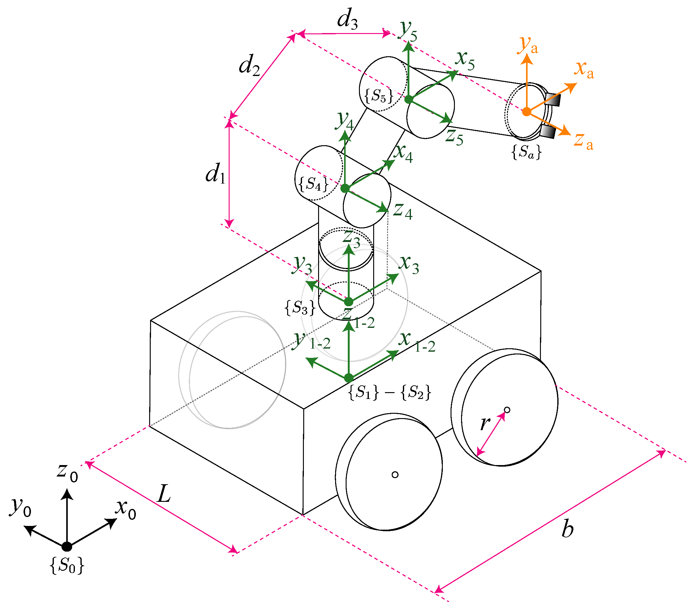
To obtain forward equations of the overall SSMM dynamics, it was considered that there is bi-directional force propagation, encompassing transmission forces both from the manipulator towards the mobile base and vice versa (see
Figure 1). This bi-directional force exchange is essential to account for the propagation of uncertainties and external disturbances such as the navigation terrain throughout the mobile robot. The Newton-Euler formulation [
64] was used in this study to set momentum and forces acting on each arm joint as a function of the state variables, external forces and constraints.
The robot base was considered as joint that can simultaneously possess both rotational and translacional motion dynamics. To apply the recursive N-E method, it was necessary to obtain the Denavit-Hartenberg (DH) parameters for a 5 DoF mobile manipulator [
64]. The DH convention allowed a homogeneous transformation matrix that described the position and orientation of a
i-th link with reference to the previous one
. Such matrix is formed by the product of 2 translation and 2 rotational transformations [
64]. In this paper, the transformation matrix is denoted by
, where
j represents the actual link respect to the
i link for a fixed coordinate axis. The DH convention designated values of rotation and translation between local coordinate axis, as specified in
Table 1 and
Figure 1. Then, the position vector for the SSMM is defined by:
where the orientation and translation of the mobile base are described by
and
. Movement of the robot arm joints is given by angular coordinates
,
, and
. Distances of each link are
, as shown in
Figure 1. Arm positions are
in
coordinates. Then, the variables
q and
denote states of position and speed for the robotic arm and base, respectively. Such varialbes are used to defined the nonlinear state space model for SSMM.
In the SSMM used in this work, the rotational and translational motion of the robot base are considered as two additional DoF. As a result, frames
and
overlap at the same coordinate origin (see
Figure 1). To apply the N-E procedure, it was necessary to obtain the rotation matrix and its inverse. Since the base reference frame
had the same orientation as the global reference frame
, the rotation matrix and its inverse are the identity matrix. Moreover, the system of the basis
is located at the center of gravity, which is also the gravity center of the mobile base. Both coordinate systems were aligned with the reference frame of the robot base and did not required rotation. Therefore, the vector
was equal to zero.
The proposed methodology used force and angular momentum equations to describe motion dynamics. Thus, it was necessary to obtain angular speed
and accelerations
of the robotic mobile base. These speed vectors were obtained as follows:
where
R is the rotation matrix, and
is the auxiliary transformation vector. To calculate the linear acceleration of the robotic system, it was considered that the mobile base exhibits translational motion, speed, and linear acceleration along the x-axis. Consequently, the
-vector in this case has to be
. Thus, the linear acceleration of the robot base could be expressed by Eq. (
4).
To obtain joint torques at the arm and base of mobile manipulator, it was assumed that the mobile base performed both rotational and translational motion concurrently. Then, the linear force in the new coordinate frame is as follows:
where
f denotes forces, and
T is transfer function. The forces and torques transferred from the manipulator to the base are included forces in both directions, from the manipulator to the base and vice versa. Considering both the joints and the mobile base, the resultant matrix becomes:
where
M,
C,
G, and
are mass, inertia matrix, Coriolis matrix, and the gravitational forces vector, and input torque vector of each joint, respectively.
The nonlinear states space
used in the proposed robust motion controller is then as follows:
where is the state vector of the nonlinear system represented in state space; is the input control vector, and is the output vector of the SSMM.
The dynamic model disregards motion constraints such as workspace limitations, environmental interactions, and payload capacity. Instead, dynamic and kinematic constraints are accounted in the proposed control strategy. As a result, it is assumed that joints cannot achieve a full range of motion control. The arm’s workspace is restricted by the lengths of its links and the geometric constraints of the mobile base. Additionally, the maximum speeds of the motors associated with the wheels and joints are given by the specifications of the mechanical actuators, while a maximum payload is set to prevent structural damage.
4. Nonlinear Model Predictive Control Strategy
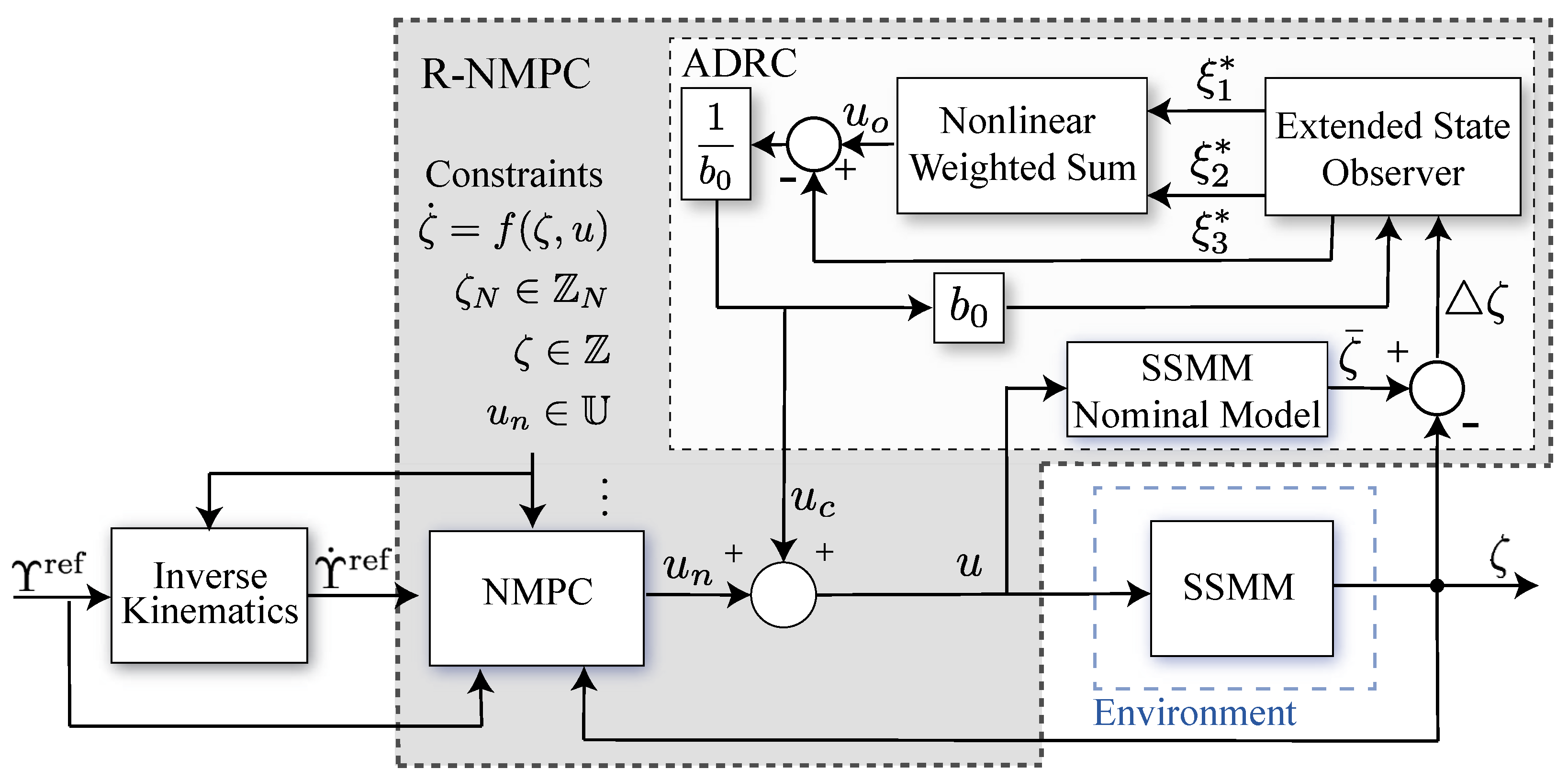
This Section describes the control architecture layout of the robust NMPC (R-NMPC) approach, encompassing the nominal controller (disturbance-free) and the ancillary control strategy designed to complement the nominal one and mitigate uncertainties and terrain disturbances, as illustrated in
Figure 2. This Section presents the dynamic model of motion for the SSMM and details the wheel-terrain interaction between the mobile base and the attached manipulator, which is also integrated into the prediction model for the proposed controller. A 3D reference trajectory is proposed for the manipulator and a 2D reference trajectory for the mobile base. Inverse kinematics is then applied to generate rotational and translational speed, which completes the references of the robotic arm and the wheels of the mobile base. Constraints are imposed taking into account the range of motion of the joint coordinates, as well as the maximum speed achievable by the physical elements of the robot. The NMPC controller uses the reference trajectory, constraints, and system outputs to optimize nominal inputs
. The NMPC stategy is addressed to control position and orientation of the mobile base and robotic arm. Furthermore, an additional strategy based on ADRC is developed to obtain the complementary control action
, which incorporates the error model to compensate for potential uncertainties and modeling errors. The combination of the predictive controller and its compensator results in a robust control signal
u according to the Eq. (
8).
The NMPC strategy uses the nonlinear dynamic model of the SSMM, as set by Eq. (
7) to predict the future system response in a finite prediction horizon
N. A control sequence is optimized in accordance with the minimization of the cost function, whereby the tracking error is subject to a state and control input constraints. Moreover, the control system uses prescribed references for position and orientation trajectories of the SSMM, constraints according to model boundaries, and the actuators of the robotic system (see
Figure 2). The NMPC uses the sliding horizon technique, which solves an optimization problem along the
N horizon that is continuously updated at each time instant. The solution of the optimization problem provides an optimized sequence of control actions
. However, only the first control action of this sequence is applied to the robotic system. The optimization problem is given by:
with:
where
denotes time horizon for an
N number of predictions;
and
are positive definite matrices weighting control objectives of the cost function
J. The cost function
J is associated with predetermined trajectory tracking objectives. The matrix
imposes penalty on the trajectory tracking errors
, thereby enabling prioritization of tracking of the mobile base over the control effort on the robotic arm. Matrix
penalizes the control input effort, minimizing abrupt changes in the control actions. On the other hand,
is the terminal cost function, which in charge of guarantee to achieve global optimal responses. In this paper
is defined for the position and orientation coordinates of SSMM with the objective of penalizing the controlled system states at the end of the prediction horizon. The function
addresses the system towards the reference and converge to zero error. The system states are constrained based on the physical limits of the SSMR joints. The mobile base can translate and rotate without restrictions, beyond that of lateral motion constraints. However, the joints of the robotic arm are constrained by their physical construction, requiring a range of operation. Constraints on the control inputs are set according to the maximum value that can be driven on each motor associated with wheels and joints of the SSMM. The mechanical coupling of the SSMM generates a bidirectional distribution of disturbances, demanding an additional constraint in the optimization problem to ensure system convergence. This constraint is closely related to the concept of passivity, which asserts that a system must not generate more energy than it receives. By incorporating this passivity constraint, the optimization process effectively handles energy exchange within the system, thereby enhancing stability and ensuring that the controlled system can robustly handle disturbances without exhibiting unstable behaviour.
The interaction between an input control space
to an output space
has been defined by Eq. (
7). With that consideration and using the definition of Hatanaka [
22], the robotic system is set to be passive if there exists a positive semi-definite storage function
V such that the following inequality is satisfied:
Equation (
10) is required to all
when the set
satisfies the system dynamics of Eq.
7. If
V is differentiable as a function of time, then inequality in (
10) can be written by:
Accounging for the dynamic system of the SSMM with 5 DoF, as defined by Equation (
7), the gravity vector
G is found to have a relationship with the potential energy matrix
P, as defined through Eq. (
12) [
22].
The sum of the kinetic energy and the potential energy
P of the robotic system is used to define the storage function
V as follows:
Then, the time derivative of
V satisfies:
Equation (
14) is used to determine the passivity function of the SSMM from torque input
at joint speed
. Then, the inequality constraint (
11) is satisfied, and the last equality constraint in (
14) may be integrated into the optimization problem (
9) to minimize the input control
.
5. Passivity-Based Robust Control Strategy
The proposed robust controller was designed to be able to maintain suitable robust performance even in the presence of external disturbances, variations of system parameters, and mismatch model errors. Robust control strategies set up an operating range that limits the extent to which the controller can mitigate adverse effects on the robotic system. Such range prevents the analysis and algorithms used from becoming excessively complex. This work examines the operating range for robustness testing in relation to the variation of model parameters. In particular, the impact of varying the inertia and mass values of the mobile manipulator components is examined. In addition, external disturbances that could impact on the robot speed when the mobile base is displaced over terrain is also addressed. Such disturbances are related to the terrain type, sliding, presence of rocks or skidding situations, and reflect the terra-mechanical interaction between the wheel and the surface.
The ADRC strategy is particularly suitable for multi-input/multi-output (MIMO) systems, especially when certain parameters remain unknown. In this paper, the ADRC approach is used as a compensator based on the error model. The core concept of ADRC involves encapsulating the unmodeled or unknown dynamics of the robotic system as a total disturbance, which is subsequently estimated and actively compensated using an Extended State Observer (ESO)-based controller [
24,
62]. The ADRC control loop, as proposed by [
24], consists of three key components: i) a transient profile generator, ii) an ESO, and iii) a disturbance rejection law. The initial component of the ADRC strategy takes as input the reference
r and generates a transient profile from the reference,
, and its derivatives
[
58]. Within the proposed controller, the compensator is designed to address the discrepancies between the nominal model and the actual response of the SSMM. Ideally, when the error is zero, the transient profile generator component can be omitted, allowing the ESO to directly provide estimated state information to generate the control output.
An ESO is designed here to estimate the robotic system output, its derivative and disturbances including external disturbances and unmodeled system dynamics. In the proposed strategy, an ESO requires a nominal model, which represents the SSMM system response without disturbances or uncertainties. The uncertainty-free model is then described as follows:
where
is the nominal state vector;
is the nominal input control vector of the SSMM. The error model is defined by the difference between the real system (
7) and nominal model (
15). Hence, The difference between the SSMM and the nominal model response generate an error variable
, which is defined by Eq. (
16). Disturbance and uncertainties information are contained in
and will be used as input for the compensator based on ADRC strategy.
Notation
is included in the variables related to the observer. Then, it is considered a state space representation for ESO, as shown in (
17):
where
w represents a weight indicating the
load disturbances affecting the system dynamics. Additionally, the parameters
and
are considered unknown, while an approximate value for the critical gain
is assumed to be available. The first two terms in the expression for
are combined into a single function, denoted by the
total disturbanceh. This term
h encompasses both
w and the discrepancy between the actual value of
and its nominal value
, formulated as:
Then, the new state space model for the ESO is as follows:
The total disturbance is unknown; therefore,
h is assigned to an additional state
. This state is estimated and compensated by the inner control loop proposed by the ADRC strategy (see
Figure 2). Thus, the extended state space model (
20) is obtained assuming that
and
is unknown:
The evolution of the system states in (
20) is obtained from the extended state observer (ESO), whose inputs correspond to the control action
acting on the state space system and measured output
, as follows:
where
denotes the estimate of the
i-th state
;
are gain coefficients, and
corresponds to nonlinear functions of the estimation error
e that define the observer correction terms. In the proposed strategy, the measured output signal is represented as
. Active reject of disturbances is achieved by subtracting the total disturbance contained in
, from the control law
, according to (
22) [
24].
Replacing (
22) in (
19) and assuming that
, the new state space system can be written as follows:
The state space model (
23) represents a disturbance-free modified model and the control action was proposed by:
Different combination of arguments makes it possible to evaluate the nonlinear expressions of the ESO according to
.
The control of system (
17) by ADRC requires the selection of the following parameters, i.e., the observer gains
, the constants
and
for the evaluation of the nonlinear observer functions, the gains
together with the constants
, as well as
for the design of the control law. The ADRC gains correspond to the bandwidth response of both the observer and the controller. However, in this work, heuristic methods are applied to determine the gains for
, which define the disturbance rejection capability of the compensator
, thus forming the proposed robust controller for the SSMM.
6. Experimental Tests and Results
This Section presents results of trajectory tracking tests conducted in a 5 DoF SSMM. Three trajectories have been proposed: i) squared-type, ii) circle-type, and iii) Lemniscata-type trajectories. The square trajectory enables the assessment of abrupt orientation changes of the robot when reaching corners. The other two trajectories allow to assess the SSMR response for recurrent robot position and orientation changes over time. This test is aimed at evaluating trajectory tracking performance of the robotic arm with respect to both longitudinal tracking control and three-dimensional positioning. The assessment encompasses the mobile manipulator’s responses, along with the evaluation of the arm tracking in three-dimensional space. This entails measurement of deviations from the target coordinates. The manipulator response will be evaluated in accordance with defined travel speeds conditions, which will be considered in order to ascertain the manipulator’s performance. To tune parameters of the NMPC controller, a heuristic method was used by considering the trade-off between tracking errors and control input effort of both base and arm (see
Table 2). The matrix of weights
,
and
are used for the NMPC and R-NMPC configuration. The first five elements of the diagonal in
Q and Pn penalize the tracking error for position variables of the SSMM according to Equation (
1). The variable
is taken as a priority because it is the manipulator base and it is highly susceptible with respect to changes in the other joints. Second priority is the translational motion of the robot base. Weights of the following variables were set according to non-oscilatory and stable responses. Using a similar insights, values for the penalization of control inputs by means of
were found, prioritizing the control of the second and third joint coordinates of the SSMM. In addition, the remaining model parameters required for the ADRC compensator in the mobile base are further detailed in
Table 3. For normalization purposes [
24], the configuration parameters
and
for the observer and control were set to values less than 1. The parameter
was found based on how fast the system compensates for disturbances. The parameter
was chosen to prevent the system overshoot in the SSMM responses. The remaining parameters were chosen according to the best system response of the experimental tests.
Tests were conducted using three benchmark controllers: i) a standard PID, ii) NMPC, and iii) R-NMPC. Two principal tests were carried out with such controllers. The first one consisted of assessing performance of controllers for trajectory tracking in the presence of disturbances. Meanwhile, in the second test, a variation of the model parameters was introduced. In this case, the mass of the mobile base, its rotational inertia, and the length of the first two links of the robotic arm were modified. This second test consisted of testing robustness of the proposed controller under the presence of an inaccurate prediction model. To assess the results of the proposed robust controller and the two additional controllers, 3 performance indices were used: i) the cumulative tracking error
, ii) the total control effort
, and iii) the total cost
[
20,
23,
30]. Each performance index was obtained while controlling the mobile base and the robotic arm, denoting the robot link as sub-indices (
b) for base and (
a) for arm, respectively.
6.1. Experimental Setup
The optimization problem related to the proposed R-NMPC approach is solved using nonlinear programming. Such programming uses the
fmincon function with the Sequential Quadratic Programming (SQP) algorithm, which requires the
Optimization Toolbox in Matlab. To implement the algorithm, the Matlab software is used on a computer with an Intel® Core(TM) i7-10750H @2.6 GHz processor and 16GB of memory. For this paper, a 5 DoF skid steer mobile manipulator was used, which has a 4 wheeled mobile base mechanically coupled with a robotic arm of three links. The mechanical coupling generates bidirectional disturbances from the base by the wheel-terrain interaction to the mobile arm and vice versa. The model used in the simulation workspace was debugged in [
64].
Table 3 describes parameters of the SSMR model used here, where
is the base mass without the robotic arm;
is the mobile base inertia;
is the friction coefficient;
is the mass of each link;
is the length of each link; and
g is the gravity acceleration.
Control input constraints were set to and . In addition, state constraints were set according to rotation limits for the joint axes by , , , and .
6.2. Trajectory Tracking Test & Terrain Disturbance Rejection
A circular trajectory was used due to its recurrent variation with respect to orientation and position reference and its constant speed (see
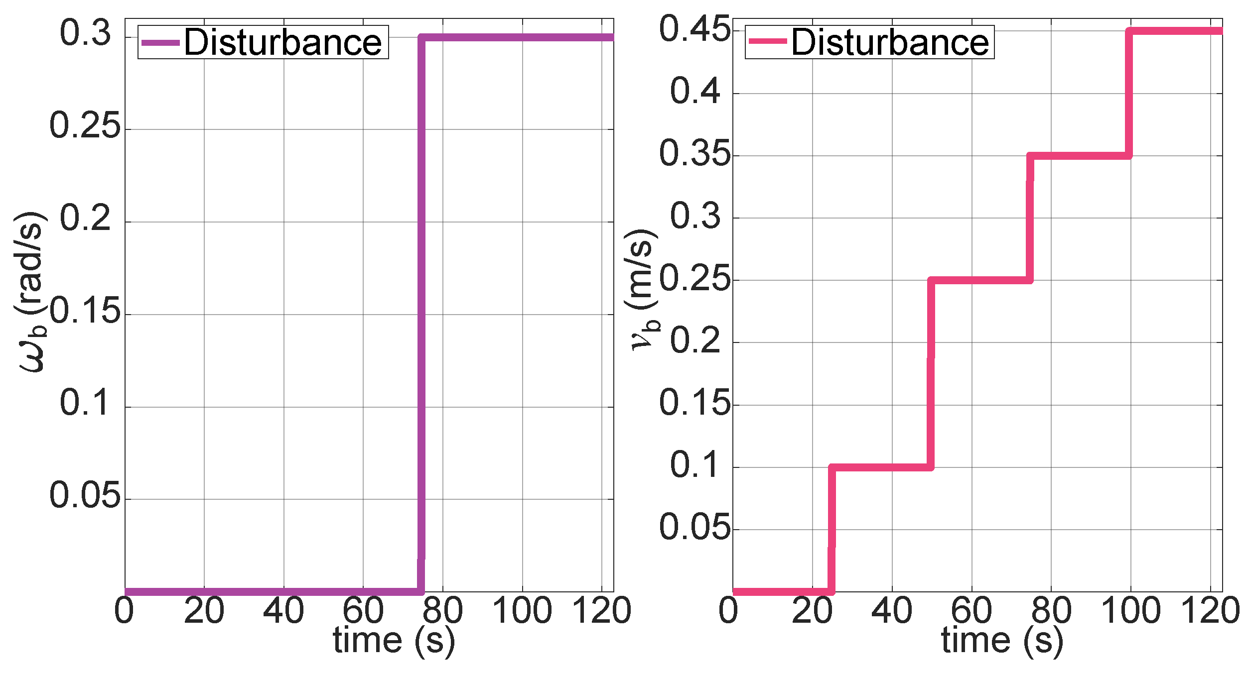
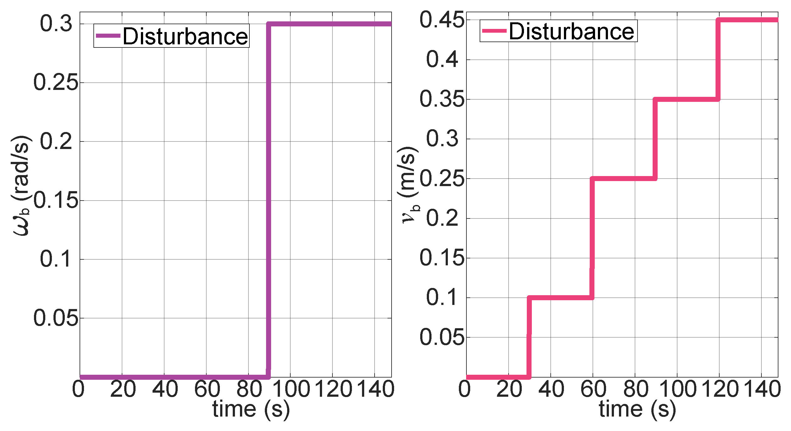
Figure 3). The aim of this evaluation is to assess performance of the robot in designated sections with terrain changes. To simulate slip corresponding to possible irregular sections through the terrain, linear and angular speed disturbances were introduced to the base of the SSMM. Linear speed disturbance was introduced at regular intervals of 20 % throughout simulation, varying in amplitude according to the vector
. On the other hand, the disturbance in angular speed was introduced under the consideration of step-type signal with amplitude 0.3
at 60 % of the total simulation time. These conditions are designed to simulate challenging terrain scenarios that the mobile manipulator would traverse to allow the base to advance toward the target and ensure that the robotic arm reaches the predetermined height. A square-type trajectory for the robotic arm was used. The reference changes of each joint coordinate introduces disturbances, which are reflected in the moving base due to its mechanical coupling. A comparative analysis of the three proposed controllers was performed to show which controller achieved the greatest reduction in tracking error.
The first trajectory to be considered for the robot base is a circle with radius of 15
m. A square trajectory with a width of 0.35
m and a height 0.25
m is used for the robotic arm. In addition, a constant speed of 0.5
is considered for the calculation of position and orientation coordinates.
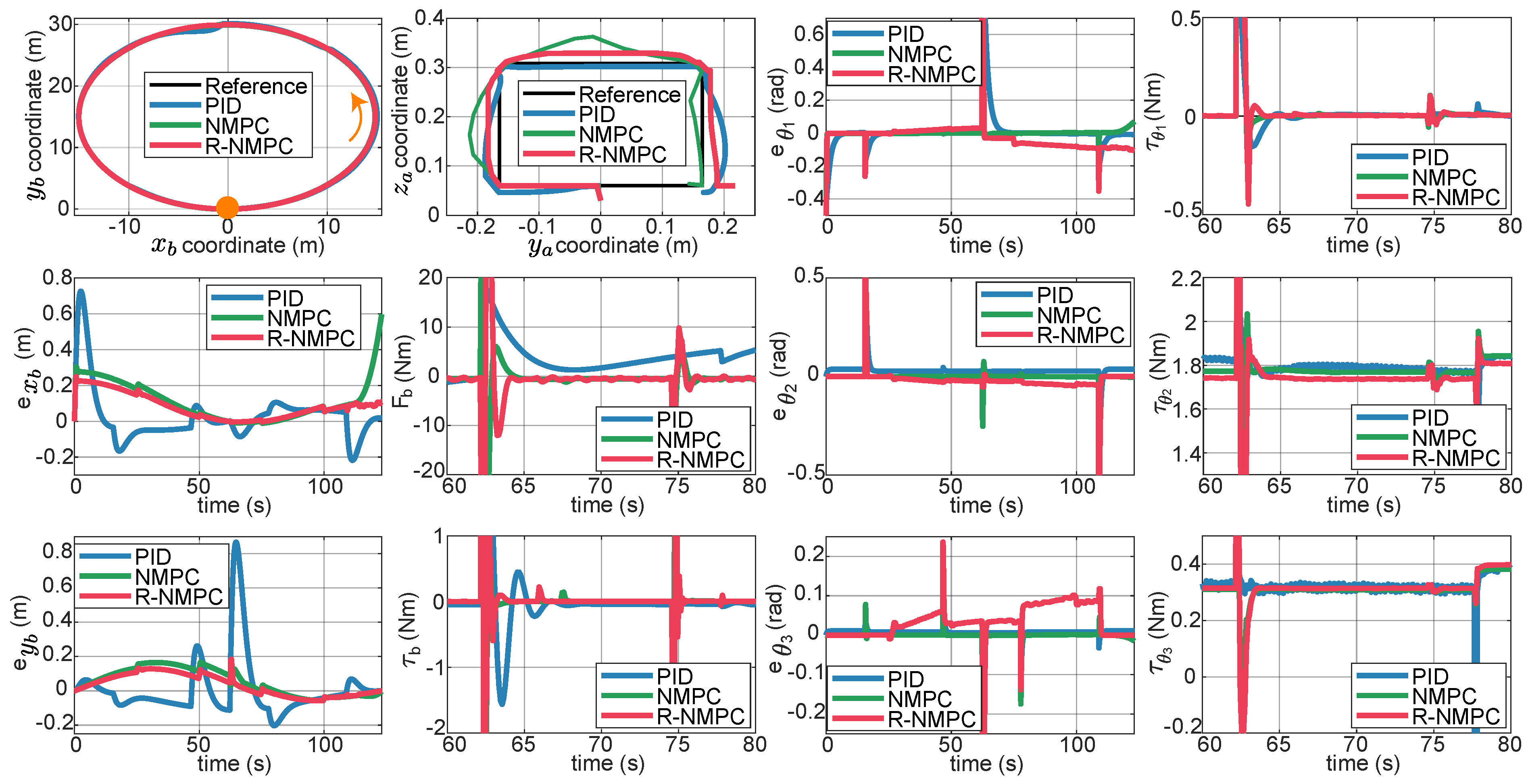
Figure 4 and
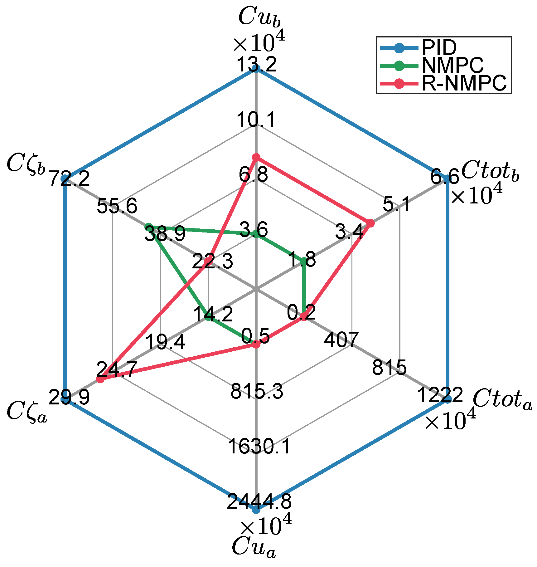
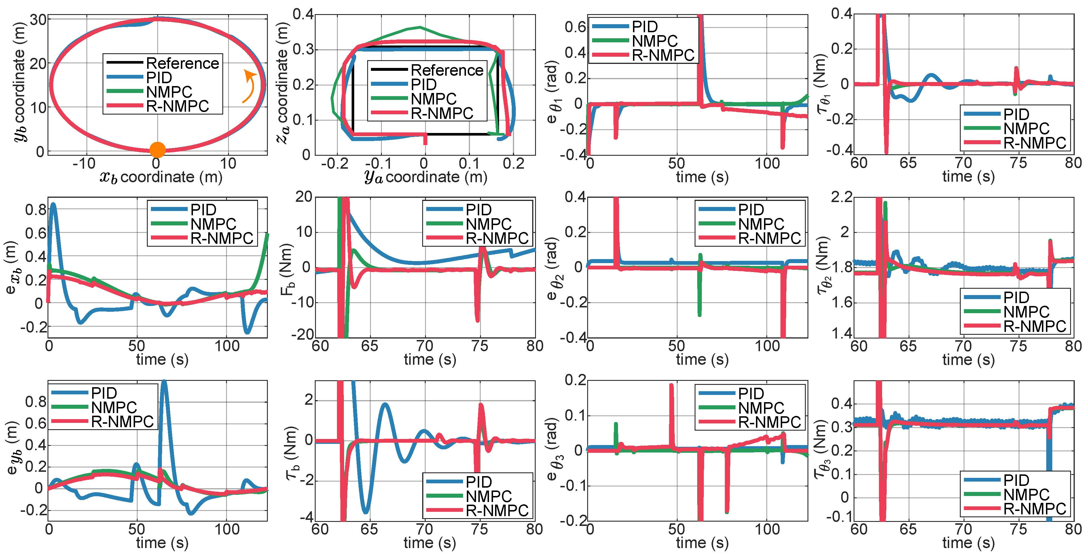
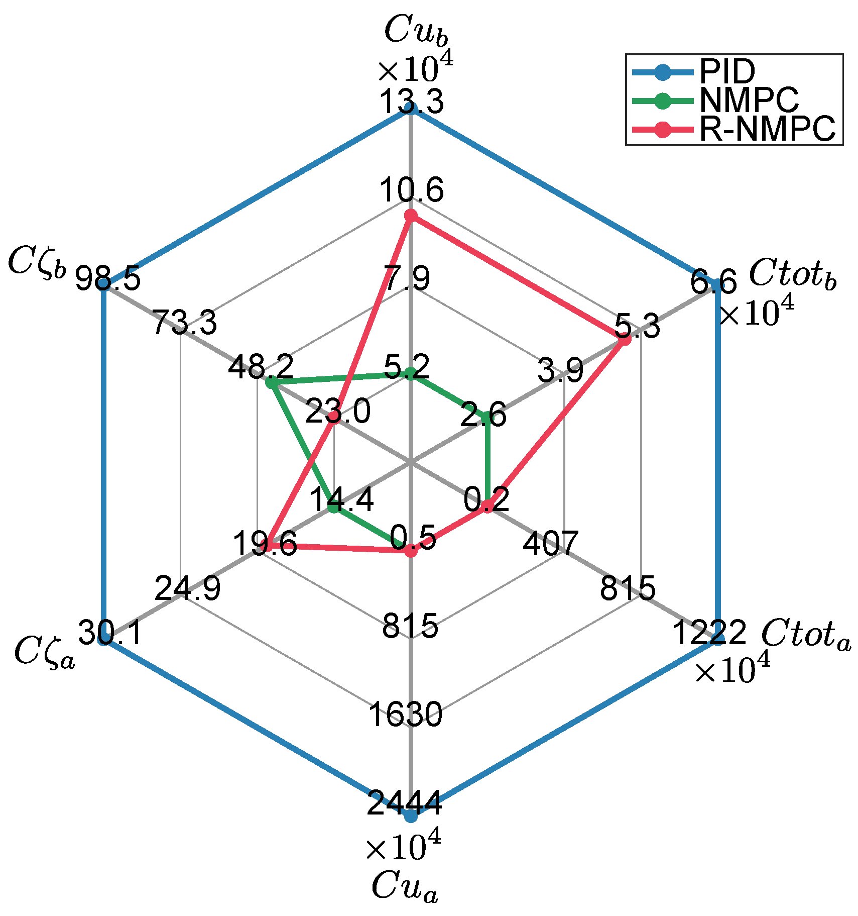
Figure 5 show trajectories an performance metrics achieved by the three controllers under analysis. It is important to note that a portion of total test time is extracted to show the transient response of the control signal performance for each signal. Position changes in the robotic arm were given at time 15, 65, and 115 (s), which caused an overshoot in the tracking error of the robotic arm and in the manipulated variable. This phenomenon is also reflected in the base and is taken as the bidirectional disturbance due to the mechanical coupling. The NMPC and R-NMPC controllers minimize the effect of disturbances and prioritize trajectory tracking. Because of this, the
of NMPC and R-NMPC is smaller than PID by 40% and 69% respectively. The PID controller is the least effective rejecting disturbances. The R-NMPC is the controller with the lowest error in the positions coordinates of the mobile base (
), as shown in
Figure 5. Similarly, disturbances in the moving base are reflected in the robotic arm, but with smaller overshoots. A positional discrepancy is observed in the robotic arm’s motion under the influence of the R-NMPC. This could be attributed as the controller prioritizes the trajectory tracking of the base and partially sacrifices the performance of the joints. For this R-NMPC
is 19% higher than NMPC. Despite the control efforts to prioritize the movement on the ground (see
Figure 4), the NMPC and R-NMPC performance indexes
and
have an improvement of 72 % and 40 % compared to PID, respectively (see
Figure 5).
The second trajectory used follows a lemniscate-type trajectory, with a height of 30 m and a width of 15 m. Linear speed disturbances were introduced at regular intervals of 20% throughout the simulation, while angular speed disturbances were applied at 60% of the total simulation time (see
Figure 6). To assess abrupt changes in joint positions at corners, a square-type trajectory was maintained for the manipulator (see
Figure 7), which indirectly propagates disturbances from the mobile base to the robot arm. A time range of 30 s was selected for the time axis to better visualize the transient behavior of the control signal.
To evaluate performance of the proposed controller against unexpected disturbances, a time range between disturbances followed by a change of joint position was also set. Then, there was a more control requirement, which can be seen in
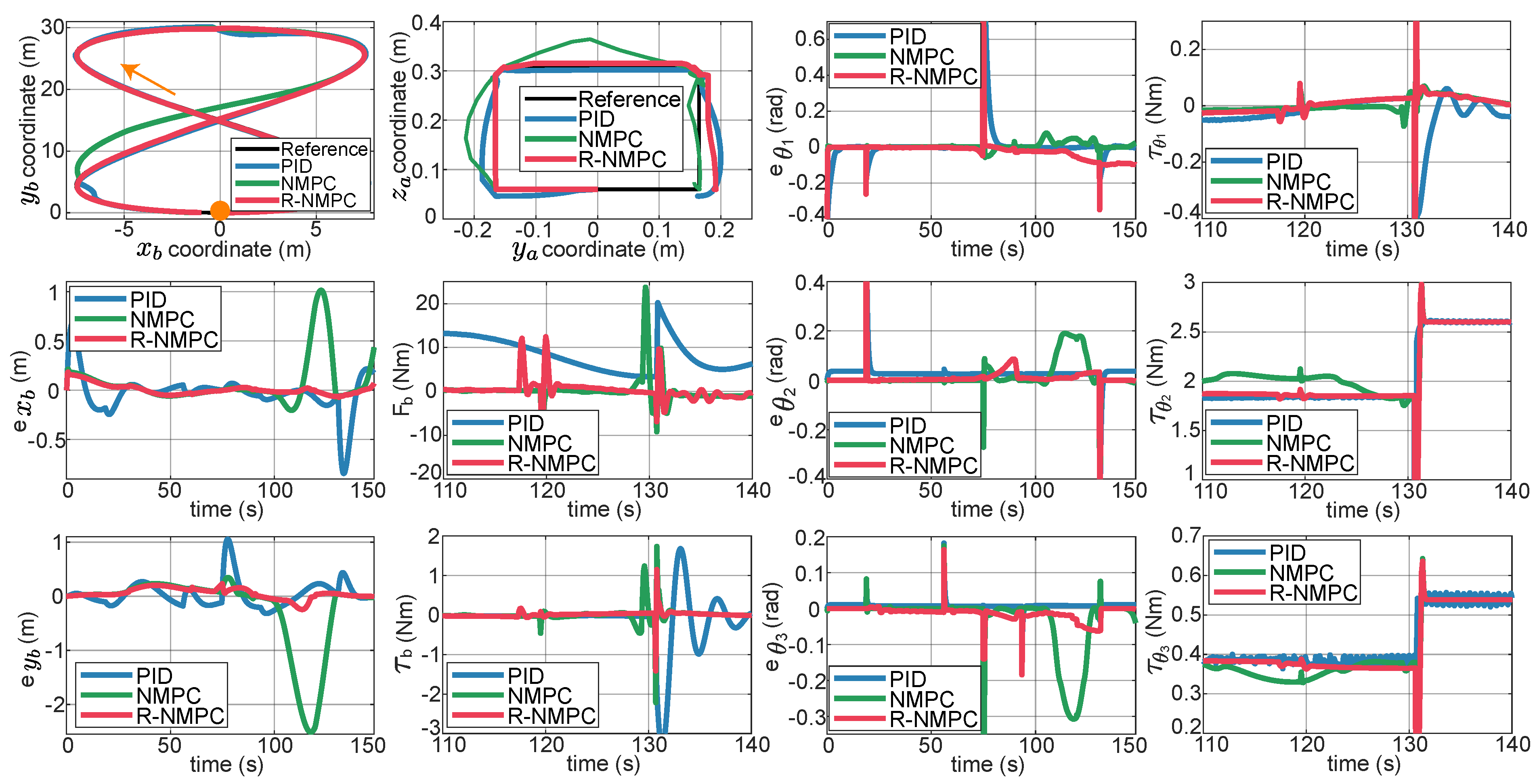
Figure 7. In this instance, it can be observed that both PID and NMPC tend to generate control responses with overshoots. On the other hand, the R-NMPC controller maintained a stable response without compromising its performance in the mobile base.
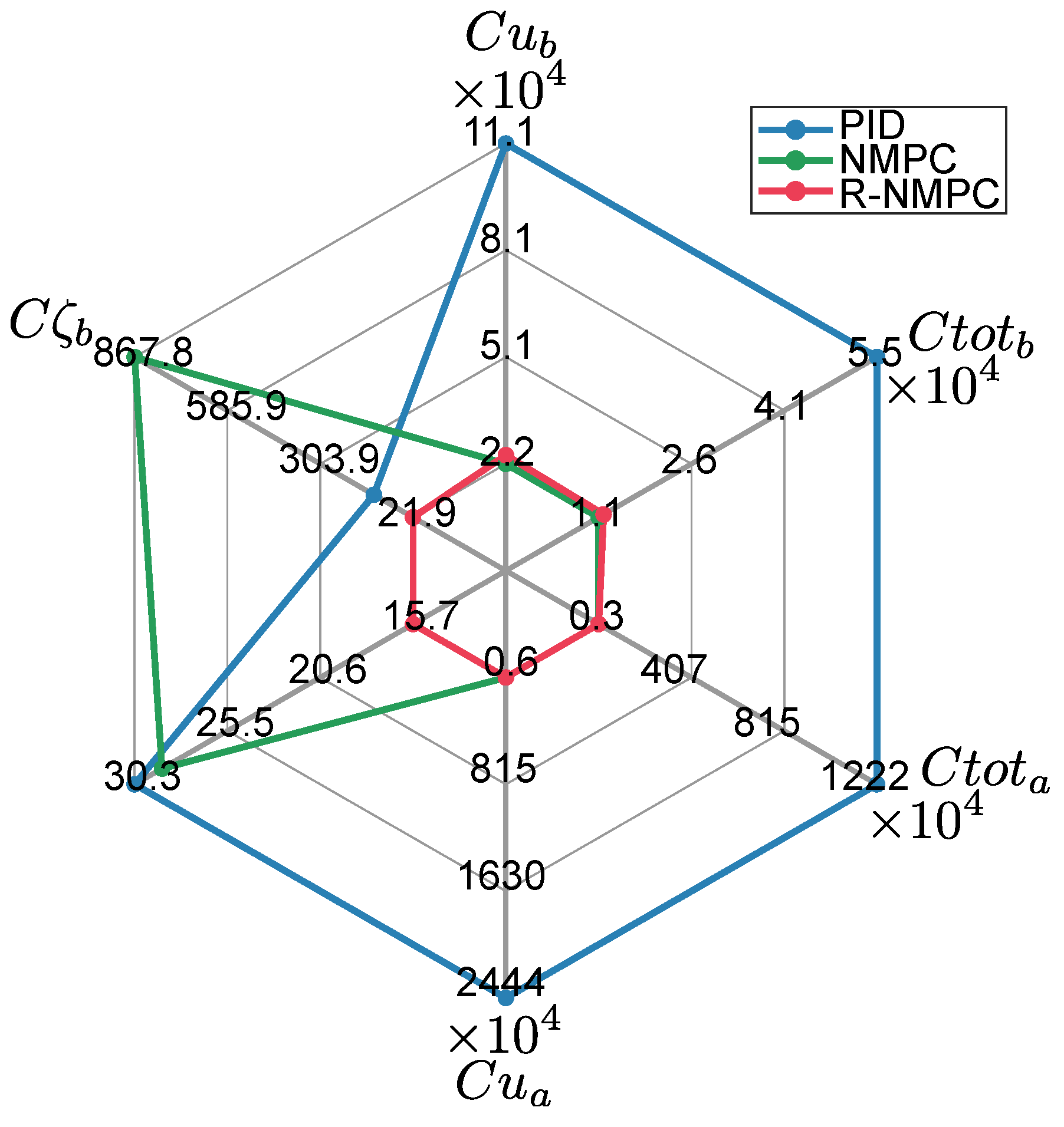
Figure 8 illustrates that the R-NMPC showed an improvement of 89 % and 79 % in terms of tracking error for the mobile base compared to the PID and NMPC, respectively. The robotic arm shows a tracking error at this time but meets prioritizing the mobile base and the reference motion on the ground.
Figure 8 shows that the R-NMPC obtained an improvement of 14 % and 27 % over the PID and NMPC in terms of tracking error for arm coordinates. With respect to the control effort, RNMPC and NMPC set a 76 % and 58 % of improvement, respectively, in comparison to PID. These values correspond to a reduction of the tracking error compensation. In both trajectory tracking tests, the R-NMPC controller demonstrated better performance while minimizing the trajectory tracking error of the mobile base. Indeed, the proposed control strategy could mitigate the impact of recurrent disturbances in the SSMR system and facilitated the generation of a less oscillatory control effort.
6.3. Test of Robustness with Model Parameter Variations
To assess performance of the robust controller, various trials wer conducted under conditions of mismatch model errors. Then, a circular, Leminscata and square trajectories were used as references for SSMM subject to model parameter variations. The same previously trajectories from
Section 6.2 were used in this test. The prediction model used in the NMPC controller and the proposed R-NMPC controller is subject to parameter variations, including a 30 % mass of mobile base and a 10 % of robotic arm, a 30 % inertia of mobile base, and a 35 % of length of the first link. Such variations comprises the maximum values under which the mobile base and arm are able to operate under feasible constraints. The introduction of an off-line parameter variation resulted in the generation of a modeling error and an increase of model uncertainty. The proposed R-NMPC controller had to be capable of compensating for such variations, thereby minimizing the tracking error and maintaining a stable control signal over time.
Tests are carried out on two trajectories for the mobile base. The first one was a circular trajectory.
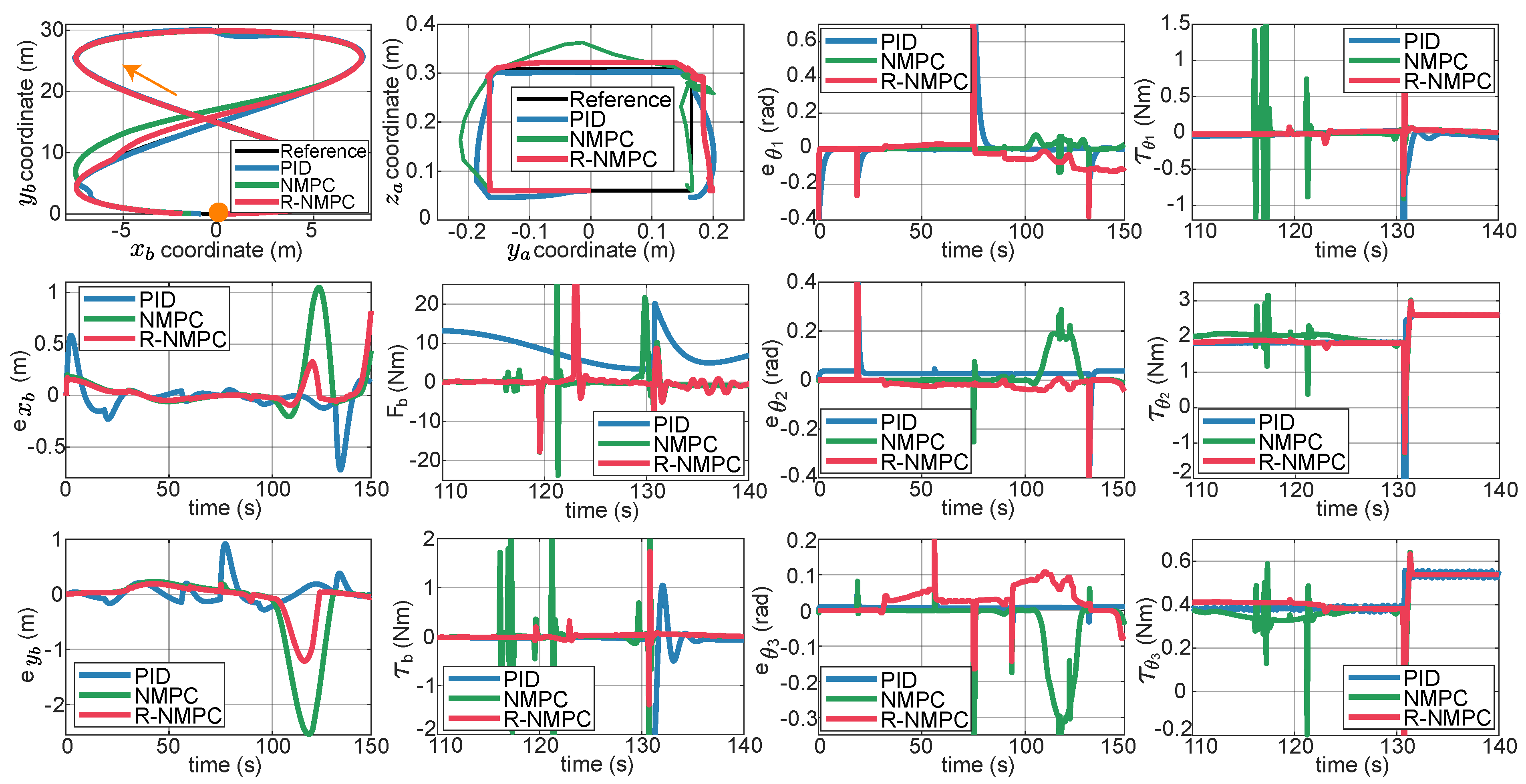
Figure 9 shows the tracking error for the mobile base. The PID controller still presented overshoots when the controlled system was affected by lineal and rotational speed disturbances, as well as under indirect disturbances caused by the motion of the robotic arm joints. The NMPC and R-NMPC mitigated this phenomenon by maintaining the tracking error close to zero. However, the NMPC tends to show larger errors and even loses efficiency. It was also shown that the tracking error in
increased up to 0.6 m, indicating that the system’s response was delayed and that it did not return to the original point. Analyzing the performance indexes (
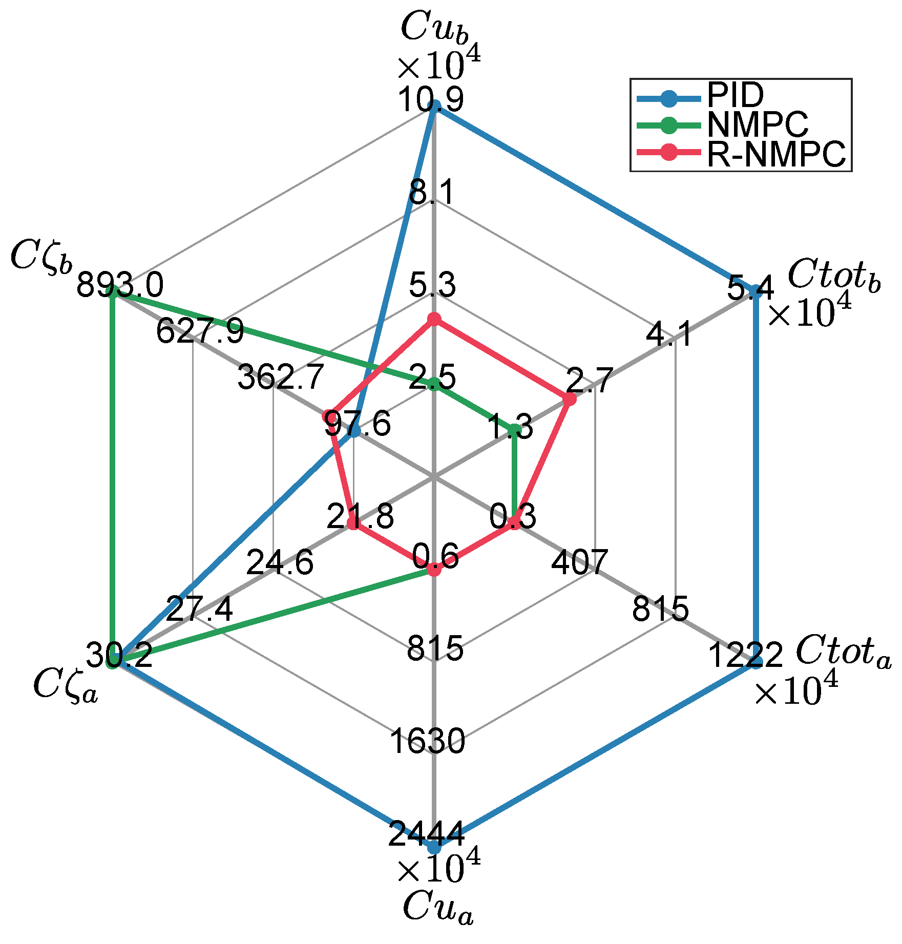
Figure 10), it can be seen that the NMPC and R-NMP controller had a 55 % and 76 % improvement, respectively, compared to the PID. In the worst-case scenario, the R-NMPC showed a reduction in tracking error for joint coordinates, with a maximum error of 0.1 rad when prioritizing base trajectory tracking.
Figure 9 demonstrated that the R-NMPC controller achieved smaller overshoots compared to NMPC and PID controllers. Overall, the proposed controller maintained the tracking error near zero during all the simulation test. Analyzing the total tracking error,
Figure 10 shows that NMPC and R-NMPC achieve improvements of 52% and 37% over PID, respectively.
Figure 9 illustrates the controlled system response between 60 and 80 s. It was shown that the PID controller exhibited larger overshoots and oscillations compared to the predictive controllers, a behaviour that also raised in the joint control signals of the robotic arm. When analyzing these control efforts, NMPC and R-NMPC demonstrated improvement of 60% and 24%, respectively, over the PID controller for the mobile base, resulting in lower values in their control signals.
Figure 10 shows that the control effort of the R-NMPC is 30 % greater than that of the NMPC. This corresponds to the effort required to minimize the trajectory tracking error. In addition, the control effort for the joints of the robotic arm, the NMPC and R-NMPC present an improvement of 90 % with respect to the PID.
Figure 9 shows that the R-NMPC control signals present reduced oscillations and more stable curves over time.
The second trajectory for the mobile base follows a Lemniscate-type reference trajectory.
Figure 11 illustrates performance of the three controllers along such path. In this scenario, the NMPC controller begins to deviate from the reference at approximately 100 s, as evidenced by tracking errors in the
and
coordinates. Speed disturbances, bidirectional disturbances, and modeling inaccuracies inhibit the NMPC from maintaining proper control. However, the R-NMPC compensated for these disturbances and modeling errors, then reducing tracking errors.
Figure 12 indicates that both the PID and R-NMPC controllers yield improvements of 80% and 95%, respectively, over NMPC, effectively mantaining the mobile base close to its reference. Additionally, due to mechanical coupling, disturbances in the mobile base trajectory affect the robotic arm’s response, resulting in oscillations, particularly at the third corner of the square trajectory.
Figure 11 shows that the NMPC controller produced tracking errors up to 0.3 rad, with overshoots exceeding those of the PID. Analysis of performance in
Figure 12 further demonstrated that the R-NMPC achieved a 48% improvement in tracking error over the PID, while the NMPC provides only a 4% enhancement.
Figure 11 shows the response of the controllers under analysis. In the mobile base, the PID generates oscillatory control efforts in the presence of disturbances. The NMPC and R-NMPC tend to generate responses with overshoot. However, NMPC presented a more abrupt response that affects the overall system performance.
Figure 11 shows that the performance index related to the control effort on the robot base for NMPC and R-NMPC presented an improvement of 81 % and 79 %, respectively, with respect to the PID. On the other hand, in the robotic arm the control efforts of the NMPC and R-NMPC show a relevant improvement in comparison with the PID. The R-NMPC applied to the mobile manipulator outperformed the other test controllers with respect to trajectory tracking at the base, despite minimal addition of control effort.
Figure 1.
Local coordinate systems and DH considerations of the SSMM.
Figure 1.
Local coordinate systems and DH considerations of the SSMM.
Figure 2.
The proposed Robust Nonlinear Model Predictive Control (R-NMPC) structure.
Figure 2.
The proposed Robust Nonlinear Model Predictive Control (R-NMPC) structure.
Figure 3.
Characterization of disturbances used in tests using circular-type reference trajectory.
Figure 3.
Characterization of disturbances used in tests using circular-type reference trajectory.
Figure 4.
Tracking tests were also considered on a circular trajectory profiling linear and angular speed disturbances on the mobile base and the robotic arm motion. The first top row from left to right depicts results of tracking a reference trajectory for the mobile base, robot arm. In the next two figures it is shown the tracking error in the joint coordinate and the control effort on the joint coordinate . The second row from left to right shows the tracking error in the x-coordinate of the mobile base, the control effort for the linear displacement of the mobile base, the tracking error of the joint coordinate , the control effort of the joint coordinate . The third row from left to right presents the tracking error in the y-coordinate of the mobile base, the control effort for the angular displacement of the mobile base, tracking error of the joint coordinate , the control effort of the joint coordinate .
Figure 5.
Results of performance indexes. Tracking tests for circular trajectory considering linear and angular speed disturbances in the mobile base. The indices correspond to the mobile base and the indices correspond to the robotic arm of the SSMM.
Figure 5.
Results of performance indexes. Tracking tests for circular trajectory considering linear and angular speed disturbances in the mobile base. The indices correspond to the mobile base and the indices correspond to the robotic arm of the SSMM.
Figure 6.
Disturbances used while testing the Lemniscata-type trajectory.
Figure 6.
Disturbances used while testing the Lemniscata-type trajectory.
Figure 7.
Tracking tests on a Lemniscata trajectory considering linear and angular speed disturbances on the mobile base and the influence of the robotic arm motion. The first top row from left to right consists of: the trajectory of the mobile base, the trajectory of the robotic arm, the tracking error in the joint coordinate , the control effort of the joint coordinate . The second row from left to right has: the tracking error in the x-coordinate of the mobile base, the control effort for the linear displacement of the mobile base, the tracking error of the joint coordinate , the control effort of the joint coordinate . The third row from left to right consists of: the tracking error in the y-coordinate of the mobile base, the control effort for the angular displacement of the mobile base, tracking error of the joint coordinate , the control effort of the joint coordinate .
Figure 8.
Performance index: Tracking tests for Lemniscata trajectory considering linear and angular speed disturbances in the mobile base. The indices correspond to the mobile base and the indices correspond to the robotic arm of the SSMM.
Figure 8.
Performance index: Tracking tests for Lemniscata trajectory considering linear and angular speed disturbances in the mobile base. The indices correspond to the mobile base and the indices correspond to the robotic arm of the SSMM.
Figure 9.
Robustness tests on a circular trajectory considering linear and angular speed disturbances on the mobile base, the influence of the robotic arm motion, and parameter variation. The first top row from left to right consists of: the trajectory of the mobile base, the trajectory of the robotic arm, the tracking error in the joint coordinate , the control effort in the joint coordinate . The second row from left to right has: the tracking error in the x-coordinate of the mobile base, the control effort for the linear displacement of the mobile base, the tracking error of the joint coordinate , the control effort of the joint coordinate . The third row from left to right consists of: the tracking error in the y-coordinate of the mobile base, the control effort for the angular displacement of the mobile base, tracking error of the joint coordinate , the control effort of the joint coordinate .
Figure 10.
Performance index: Robustness tests for circular trajectory considering linear and angular speed disturbances and parameter variations in the mobile base. The indices correspond to the mobile base and the indices correspond to the robotic arm of the SSMM.
Figure 10.
Performance index: Robustness tests for circular trajectory considering linear and angular speed disturbances and parameter variations in the mobile base. The indices correspond to the mobile base and the indices correspond to the robotic arm of the SSMM.
Figure 11.
Robustness tests on a Lemniscata trajectory considering linear and angular speed disturbances on the mobile base, the influence of the robotic arm motion, and parameter variation. The first top row from left to right consists of: the trajectory of the mobile base, the trajectory of the robotic arm, the tracking error in the joint coordinate , the control effort in the joint coordinate . The second row from left to right has: the tracking error in the x-coordinate of the mobile base, the control effort for the linear displacement of the mobile base, the tracking error of the joint coordinate , the control effort of the joint coordinate . The third row from left to right consists of: the tracking error in the y-coordinate of the mobile base, the control effort for the angular displacement of the mobile base, tracking error of the joint coordinate , the control effort of the joint coordinate .
Figure 12.
Performance index: Robustness tests for Lemniscata trajectory considering linear and angular speed disturbances and parameter variations in the mobile base. The indices correspond to the mobile base and the indices correspond to the robotic arm of the SSMM.
Figure 12.
Performance index: Robustness tests for Lemniscata trajectory considering linear and angular speed disturbances and parameter variations in the mobile base. The indices correspond to the mobile base and the indices correspond to the robotic arm of the SSMM.
Table 1.
Denavit-Hartenberg parameters for the SSMM robot.
Table 1.
Denavit-Hartenberg parameters for the SSMM robot.
| i |
Articulation |
|
|
|
|
| 1 |
Mobile base |
0 |
0 |
0 |
0 |
| 2 |
Auxiliary joint |
0 |
0 |
0 |
0 |
| 3 |
Manipulator base |
|
|
0 |
|
| 4 |
Shoulder joint |
|
0 |
|
0 |
| 5 |
Arm joint |
|
0 |
|
0 |
Table 2.
Weight matrices and configuration parameters used in NMPC and R-NMPC.
Table 2.
Weight matrices and configuration parameters used in NMPC and R-NMPC.
| Weight Matrix |
Values |
|
diag(60, 100, 150, 70, 90, 0.1, 1, 1, 0.1, 0.1) |
|
diag(0.1,1,1,0.1,0.1) |
|
diag(60, 100, 150, 70, 90) |
|
[0.9,0.9] |
|
[1.2, 1.2] |
|
[0.2,1.2] |
|
[0.5,0.8] |
|
[1,10] |
|
[20,20] |
Table 3.
Parameter of articulated Skid-Steer Mobile Manipulador (SSMM).
Table 3.
Parameter of articulated Skid-Steer Mobile Manipulador (SSMM).
| Parameter |
Value |
Parameter |
Value |
|
12
|
|
0.5
|
|
1 |
|
0.07 |
|
0.12 |
|
0.12 |
|
0.12 |
|
2.867
|
|
0.633
|
|
0.79
|
|
0.06 m
|
|
0.019 m
|
|
0.139 m
|
g |
9.8062
|
