Preprint
Article

Mapping the Future: Climate-Induced Changes in Biomass Density Across Mexico’s Coniferous Forests

Altmetrics

Downloads

46

Views

34

Comments

0

A peer-reviewed article of this preprint also exists.

Submitted:

17 October 2024

Posted:

18 October 2024

You are already at the latest version

Alerts
Abstract
Climate variations in temperature and precipitation significantly impact forest productivity. Precipitation influences the physiology and growth of species, while temperature regulates photosynthesis, respiration, and transpiration. This study developed bioclimatic models to as-sess how climate change will affect the carbon density of aboveground biomass (cdAGB) in Mex-ico's coniferous forests for 2050 and 2070. We used cdAGB data from the National Forest and Soils Inventory (INFyS) of Mexico and 19 bioclimatic variables from WorldClim ver. 2.0. The best predictors of cdAGB were obtained using machine learning techniques with the 'caret' library in R. The model was trained with 80% of the data and validated with the remaining 20% using Generalized Linear Models (GLM). Current cdAGB prediction maps were generated using the best predictors. Future cdAGB was calculated with the average of three general circulation mod-els (GCMs) of future climate projections from the Coupled Model Intercomparison Project Phase 5 (CMIP5), under four Representative Concentration Pathways (RCPs): 2.6, 4.5, 6.0, and 8.5 W/m². The results indicate cdAGB losses in all climate scenarios, reaching up to 15 Mg C ha-1, and could occur under the RCP 8.5 scenario by 2070 in the central region of the country. Tempera-ture-related variables are more important than precipitation variables. Bioclimatic variables can explain up to 20% of the total variance in cdAGB. The temperature in the study area is expected to increase by 2.66 °C by 2050 and 3.36 °C by 2070, while precipitation is expected to fluctuate by ±10% relative to the current values, which. could geographically redistribute the cdAGB of the country's coniferous forests. These findings underscore the need for forest management to focus not only on biodiversity conservation but also on the carbon storage capacity of these ecosys-tems.
Keywords: 
Subject: Environmental and Earth Sciences  -   Environmental Science

1. Introduction

Forests occupy approximately 31% of the Earth’s terrestrial surface, equivalent to around 4.06 billion hectares, and play a pivotal role in climate regulation by acting as major carbon sinks. It is estimated that global forests sequester approximately 662 gigatonnes (Gt) of carbon, distributed as follows: 44% in living biomass, 45% in soil organic matter, and 11% in dead wood and litter [1].
In Mexico, forests cover approximately 64.8 million hectares, accounting for about 33% of the national land area [1]. These forests encompass a wide range of types, including temperate, broad-leaved, mixed, and tropical forests [2], and are estimated to store around 1.69 Gt of carbon [3]. Changes in temperature and precipitation patterns driven by climate change have been shown to adversely affect forest growth, biomass accumulation, and carbon sequestration at a global scale [4,5].
The scientific foundation for studying climate change is unequivocal, and the corresponding findings are irrefutable. Between 2011 and 2020, the global average surface temperature rose by 1.09 °C compared to the 1850-1900 baseline, with more pronounced warming observed in the Northern Hemisphere, particularly over land (1.59 °C) compared to oceans (0.88 °C). Precipitation patterns are shifting, with increases observed at higher latitudes and decreases in the subtropics. Climate extremes are projected to become more frequent and intense, while the efficiency of carbon sinks is expected to diminish [6].
In Mexico, the average temperature increased by 0.31 °C per decade between 1971 and 2020, with the most pronounced effects occurring in the northern plateau during the summer months. According to projections under the SSP3-7.0 climate scenario, the average temperature is expected to rise by 0.82 °C between 2020 and 2039, and by 1.63 °C between 2040 and 2059. Moreover, certain northern states are likely to experience significant reductions in precipitation [7].
Precipitation and temperature are well-established as primary drivers of forest biomass productivity. Precipitation plays a pivotal role in plant physiology by regulating processes such as transpiration, nutrient uptake, stomatal conductance, and nutrient availability [8,9], in addition to shaping species-specific growth strategies. Variations in precipitation availability also impact water use efficiency [10,11], creating a direct relationship between precipitation levels and biomass productivity [2].
Likewise, temperature exerts significant control over plant growth by modulating fundamental physiological processes, including photosynthesis, respiration, and transpiration [4,12]. It also governs the rate of chemical reactions and CO2 assimilation [13]. While rising temperatures may stimulate biomass accumulation in boreal forests, they tend to suppress growth in tropical forests [14]. Excessively high temperatures reduce growth rates, alter leaf pigmentation, impair root system development, and induce water stress, thereby disrupting normal growth patterns [15].
Plants from temperate climates exhibit a degree of cold tolerance, but extremely low temperatures negatively affect processes such as cell division, photosynthesis, and metabolic activity, leading to reduced productivity [16].
Climatic variations are driving forests to become increasingly dynamic systems [17], resulting in changes in tree species composition within ecosystems [11]. Simultaneous shifts in temperature and precipitation lead to either reductions or increases in ecosystem biomass, thereby altering global forest distribution patterns [18].
It has been well established that temperature exerts both positive and negative influences on aboveground forest biomass [4,19,20]. Furthermore, precipitation has been consistently shown to have a positive correlation with aboveground biomass [12,21]. These effects have been observed across various forest biomes, including temperate, tropical, and boreal ecosystems [14], as well as at the species level [8].
To estimate aboveground biomass in forest ecosystems, both dynamic variables (related to climate) and static variables (such as diameter at breast height, basal area, stand density, slope, aspect, and elevation, among others) have been jointly applied [8,22,23,24]. These mixed models, which incorporate intrinsic and extrinsic factors influencing aboveground biomass, have demonstrated moderate predictive capacity, with determination coefficients (R²) ranging from 0.19 to 0.86 [8,22,23]. In some cases, these models include nine or more explanatory variables [8].
While these models are useful in identifying correlations between biomass and environmental variables, they are limited in their ability to quantify the direct impacts of climate change on aboveground biomass [8,23,25]. Furthermore, forests are highly dynamic systems that undergo temporal changes due to natural disturbances, anthropogenic activities, and climatic fluctuations, which introduces additional complexity to the modeling process [24,26].
The research conducted by [27] indicated that, among ten conifer species, precipitation demonstrated a positive correlation with aboveground biomass density (0 ≤ ρ ≤ 0.20), whereas temperature exhibited a negative correlation (−0.20 ≤ ρ ≤ 0). Importantly, the magnitude and direction of the correlation between climatic variables and aboveground biomass in forest ecosystems are highly contingent upon several factors, such as spatial scale [28], forest type [4], and species-specific traits [12,29].
In order to deepen our understanding of how climate change specifically influences aboveground biomass, it is imperative to develop new modeling frameworks. These models should integrate dynamic climatic data to directly assess the effects of climate variability and enable future projections—an objective that cannot be fully achieved by models that rely solely on static stand or site-level variables.
Building upon the aforementioned considerations, this study's primary objective was to develop bioclimatic and dynamic models specifically designed to evaluate the impacts of climate change on the geospatial distribution of aboveground live biomass carbon density in Mexico's pine forests. The analysis incorporated four distinct climate scenarios based on Representative Concentration Pathways (RCPs) 2.6, 4.5, 6.0, and 8.5 W/m², projected for the years 2050 and 2070. These models are intended to provide highly accurate information that can enhance forest management practices and contribute to climate change mitigation efforts. It is hypothesized that the future climate projections will exert a significant influence on the aboveground biomass carbon density in the pine forests of Mexico.

2. Materials and Methods

2.1. Study Area Description

Conifers in Mexico are found from sea level up to over 4,000 m in altitude, with the highest diversity concentrated in the Sierra Madre Occidental (SMOc) and the Sierra Madre Oriental (SMO), and Mexico hosts 49 species of pine, representing 40% of the approximately 120 pine species worldwide [30]. They span approximately from 32 °N north latitude to 19 °N, and from 105 °W west longitude to 98 °W, on soils derived from igneous and metamorphic rocks [31]. These ecosystems are characterized by a temperate to cold climate, with annual precipitation ranging from 350 to 1200 mm and average temperatures ranging from 6 to 28 °C [32], with rainy summers and dry, cold winters, dominated by coniferous trees such as pines (Pinus spp.), firs (Abies spp.), cedars (Cupressus spp.), and junipers (Juniperus spp.) [33].

2.2. Data Acquisition and Cleaning Process

A total of 22 parameters including type, topographic, species richness, biomass, and carbon (aboveground and belowground), health indices, climate, geographic, and dasometric factors were obtained from [2]. From these, we used data on carbon density in aboveground live biomass (henceforth referred to as cdAGB), geographic coordinates (lat, long), and ID of each cluster, exclusively from the parameter type='coniferous forests'. The cdAGB is the carbon stock per unit area of live biomass contained in living trees, including stems, branches, leaves, and seeds [34]. These data were calculated from the National Forest and Soil Inventory (INFyS) of Mexico (2009-2012) [2]. Additionally, we utilized 19 bioclimatic variables from WorldClim version 2.0, covering the period from 1970 to 2000 (Appendix A), in raster format with a resolution of 30 arcseconds, published in January 2020 [35]. These variables have been previously used in similar studies [8,9,12,14,28,36].
Using the 'raster' library in R [37], we employed the geographic coordinates of each cluster to extract values for the 19 bioclimatic variables (Bios). To identify erroneous or atypical data in cdAGB, we applied a Principal Component Analysis (PCA) to the centered and scaled matrix of cdAGB and 19 Bios, using the 'FactoMineR' v.2.9 library [38]. We considered outliers as those falling outside the 95% confidence ellipse of the PCA, which were subsequently excluded from the dataset to ensure the coherence and reliability of the results.

2.3. Predictive Modeling of cdAGB

Due to the significant climatic variability recorded in the pine forests of the country [31], and aiming to enhance predictions of cdAGB, a bioclimatic stratification of Mexico's pine forest areas was conducted. We utilized 19 bioclimatic variables in raster format, employing the "GeoStratR" library [39], to create strata (geographical space) in the same format. The clusters from INFyS located within each generated stratum were separated for independent analysis.
For the selection of predictors (Bios) of cdAGB, within each stratum, the 'machine learning' (ML) technique employing 10-fold cross-validation was utilized, employing backward selection. A tuning grid ranging from 1 to 7 predictors (nvmax = 1:7) was considered [40]. From each subset of predictors identified by ML, the statistical significance of regression coefficients (p < 0.05) and the variance inflation factor (VIF) were evaluated to mitigate multicollinearity effects.
With the subset of predictors that met these criteria, the model was trained using the Generalized Linear Models (GLM) method with the 'identity' link function. For this purpose, 80% of the data (randomly obtained and by quantiles) from the previously cleaned matrix was used. This approach (GLM) is suitable for continuous and positive response variables [2,9] in this type of study.
The model fitting was performed using the 'caret' package in R [40]. Hypothesis tests ( = 0.05 ) were conducted on the regression coefficients ( H 0 : β i = 0 v s H 1 : β i 0 , , β i j ) of the final model. We utilized the "lmg" metric to calculate the importance of each bioclimatic variable (as a percentage of model explained variance), which provides a decomposition of the model's explained variance into non-negative contributions [41]. With the remaining 20% of the data, the model was validated using various techniques: Leave-One-Out Cross-Validation (LOOCV), Cross-Validation (CV; k=10), Repeated Cross-Validation (RCV, k=10, rep=10), and Bootstrap (reps=100). The evaluation included calculations of Root Mean Square Error (RMSE), Pseudo Coefficient of Determination (Rsquared), and Mean Absolute Error (MAE) to assess the model's performance. These validations were conducted using the 'caret' R package [40].

2.4. Current and Future Prediction and Rate of Change of cdAGB

Using the generated bioclimatic models, current predictions of cdAGB were made for each stratum, employing the corresponding bioclimatic predictors. The raster library of the R software [37] was utilized with the argument `type = "response"` to generate raster maps of cdAGB predictions.
To predict future cdAGB, raster layers from three different General Circulation Models (GCMs) were obtained: MIROC-6, GISS-E2, and CMCC-ESM2. From these models, only the bioclimatic predictors of cdAGB for each stratum were selected. The GCMs are derived from future climate projections of the Coupled Model Intercomparison Project Phase 5 (CMIP5), at a resolution of 2.5 degrees. Four Representative Concentration Pathways (RCPs) developed by the Intergovernmental Panel on Climate Change [42] were used, characterized by their projected Total Radiative Forcing (TRF) for the year 2100, ranging from 2.6, 4.5, 6.0, to 8.5 W/m², considering the years 2050 and 2070. These RCP scenarios are used to project potential future trajectories of climate change based on different emission levels and mitigation efforts.
Through raster algebra, the 3 raster layers of each GCM, RCP, and year were averaged. Using this average and the corresponding bioclimatic model, future prediction of cdAGB was conducted for each stratum. Similarly, the R raster library [37] was employed with the argument `type = "response"` to generate raster maps of future cdAGB predictions. To identify changes in future cdAGB relative to the current scenario, the following expression was used: cdAGB (future) - cdAGB (current). The results are as follows: 0 if pixel values are equal in both scenarios; positive if cdAGB is higher in the future; and negative if cdAGB is higher in the current scenario.
To visualize the vulnerable areas of Mexico's coniferous forests to changes in cdAGB due to climate change, a 40 km radius buffer was created around each site from the National Forest and Soil Inventory. This delineated the forested areas potentially affected. Subsequently, the number of pixels for each cdAGB change category or rate within these buffer polygons was quantified. The resulting change rate was then presented in map form for each RCP and year.
In addition, uncertainty in future predictions of cdAGB was quantified using the standard error: EE(θ) = √[Var(θ). This involved repeated predictions of cdAGB from MIROC-6 + GISS-E2 + CMCC-ESM2, for each RCP and year, which were averaged using the raster library (Hijmans, 2010), and generating a raster map of EE(θ).

2.5. Bioclimatic Predictors: Current Analysis and Future Projections

In order to determine the influence of future bioclimatic predictors on the changes in cdAGB of Mexican forests, the non-parametric Wilcoxon signed-rank test was employed. This test was used to evaluate whether there are significant differences between the medians of two samples: the current bioclimatic predictor and the future bioclimatic predictor (e.g., current Bio1 vs. Bio1 2050, RCP 4.0). A significance level of 95% was used.
For this purpose, the current and future values (average of 3 GCM, RCP, and year) of the predictors for each stratum (Bios) were extracted using the geographic coordinates of each cluster and employing the raster library [37]. These analyses were represented in violin plots, with temperature-derived Bios shown in orange and precipitation-derived Bios in blue, with statistical significance indicated by the * symbol at the top.
All statistical analyses, figures, and geographic processing were performed using R software [43].

3. Results

3.1. Distribution Carbon Density Of Aboveground Live Biomass

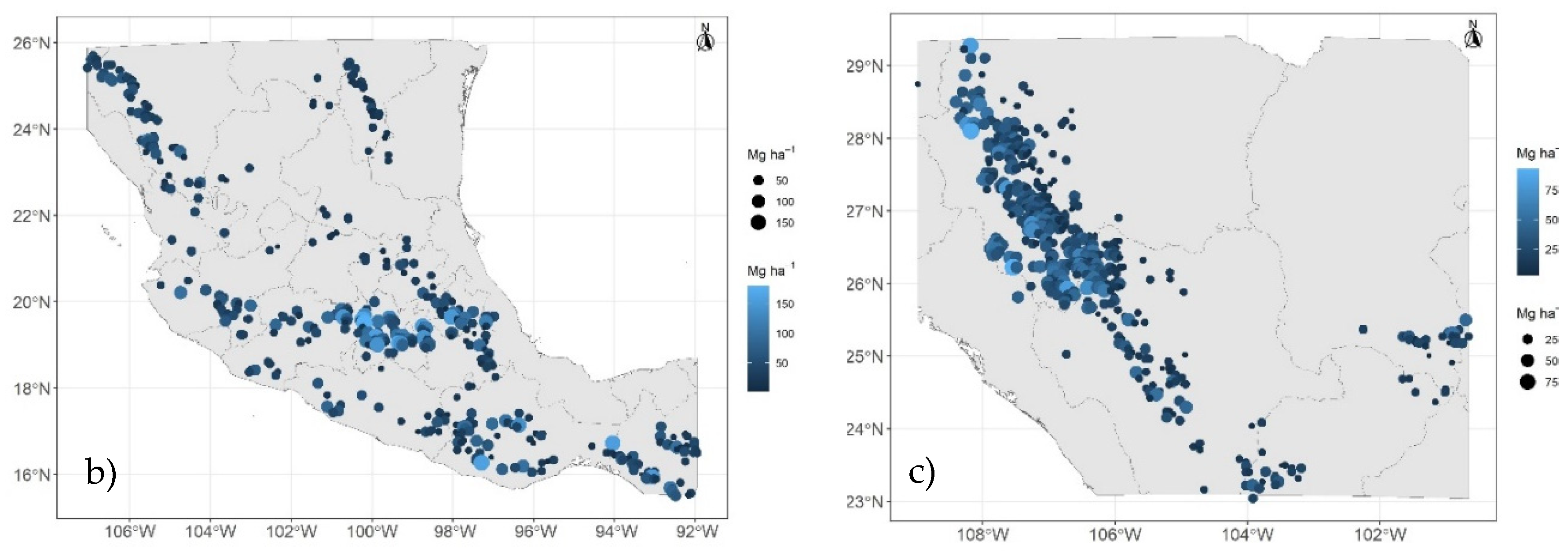
The stratification process of the coniferous forests in Mexico resulted in three strata: Stratum I, in the northwest of the country (Figure 1a; n = 60), Stratum II, in the central-southern part of the country (Figure 1b; n = 450), and Stratum III, located in the Sierra Madre Occidental, SMO (Figure 1c; n = 463).

3.2. Models For Predicting Carbon Density in the Aboveground Live Biomass

The bioclimatic variables selected by the algorithms were statistically significant (p < 0.05) for predicting cdAGB. The predictors (Bios) of cdAGB were representative of both precipitation variables (3 out of 6) and temperature variables (3 out of 6). However, at the stratum level, temperature variables are more important (Imp., Table 1) than precipitation variables. Bio 5 (Max Temperature of Warmest Month) was the best predictor of cdAGB in 2 strata (I and II). No model exhibited multicollinearity (VIF < 1.16), which ensures that cdAGB predictions are not overestimated.
The equations for estimating cdAGB in each stratum are as follows:
Stratum I: cdAGB (Mg C ha-1) = 64.8332 + -0.1897*Bio 5 (°C x10) + 0.0586*Bio 18 (mm)
Stratum II: cdAGB (Mg C ha-1) = 87.6362 + -0.2572*Bio 5 (°C x10) + 0.0190*Bio 12 (mm)
Stratum III: cdAGB (Mg C ha-1) = 26.6379 + -0.0959*Bio 10 (°C x10) + 0.0933*Bio 13 (mm)
The mean of cdAGB does not follow a pattern among strata; that is, it is not lower in stratum I and higher in stratum III. The mean cdAGB in stratum II represents, on average, up to 1.6 times more than in strata I and III; and it ranges from 23.14 Mg C ha-1 (stratum I) to 42.57 Mg C ha-1 (stratum II), with maximum values reaching almost 180 Mg C ha-1 (Table 2), but it also has the highest variability (CV > 60%). None of the variables showed normality (p < 0.0001) according to the Shapiro-Wilk and Anderson-Darling tests (Table 2).

3.3. Validation of Predictive Models for cdAGB

According to the pseudo R² derived from the validation procedure, bioclimatic variables explain an average of 19% of the cdAGB (Table 3). The LOOCV method calculates the lowest R² (0.10), while the other methods yield an average R² of 0.22. According to the validation, when using the models to predict aboveground biomass carbon density with independent data from the training set, the estimation errors (RMSE) could range from 13.18 Mg C ha⁻¹ (stratum III) to 42.42 Mg C ha⁻¹ (stratum I), with the best estimates observed in stratum III.

3.4. Current And Future Prediction of Carbon Density of Aboveground Live Biomass

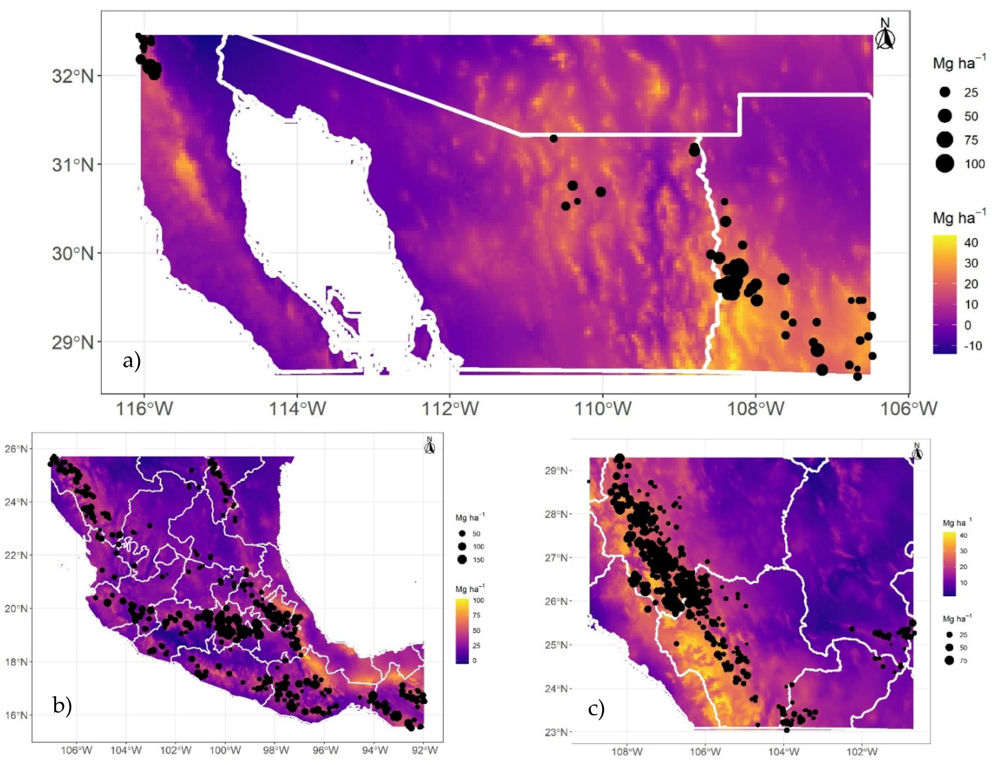
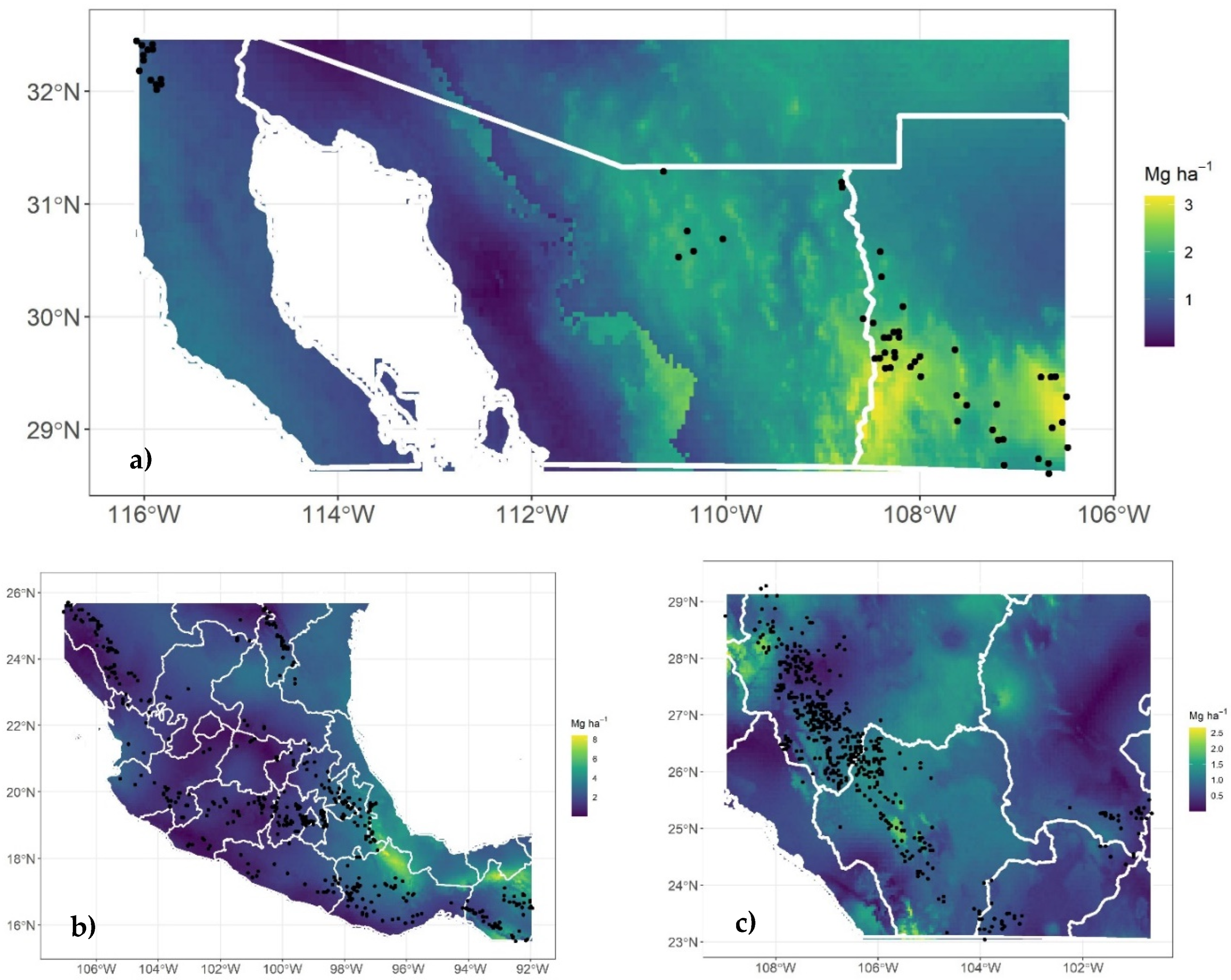
Using the bioclimatic models generated here, at the INFyS sites, predictions range from 7.48 to 34.79 Mg C ha-1; from 16.68 to 71.29 Mg C ha-1; and from 10.98 to 41.91 Mg C ha-1 for strata I, II, and III, respectively (Figure 2a-Figure 2c). The highest cdAGB is observed/predicted in stratum II (Figure 2b) in the central region of the country. The highest differences between observed cdAGB – estimated cdAGB are -19 and +30; -52 and +124; -29 and +56 Mg C ha-1, respectively for strata I, II and III.
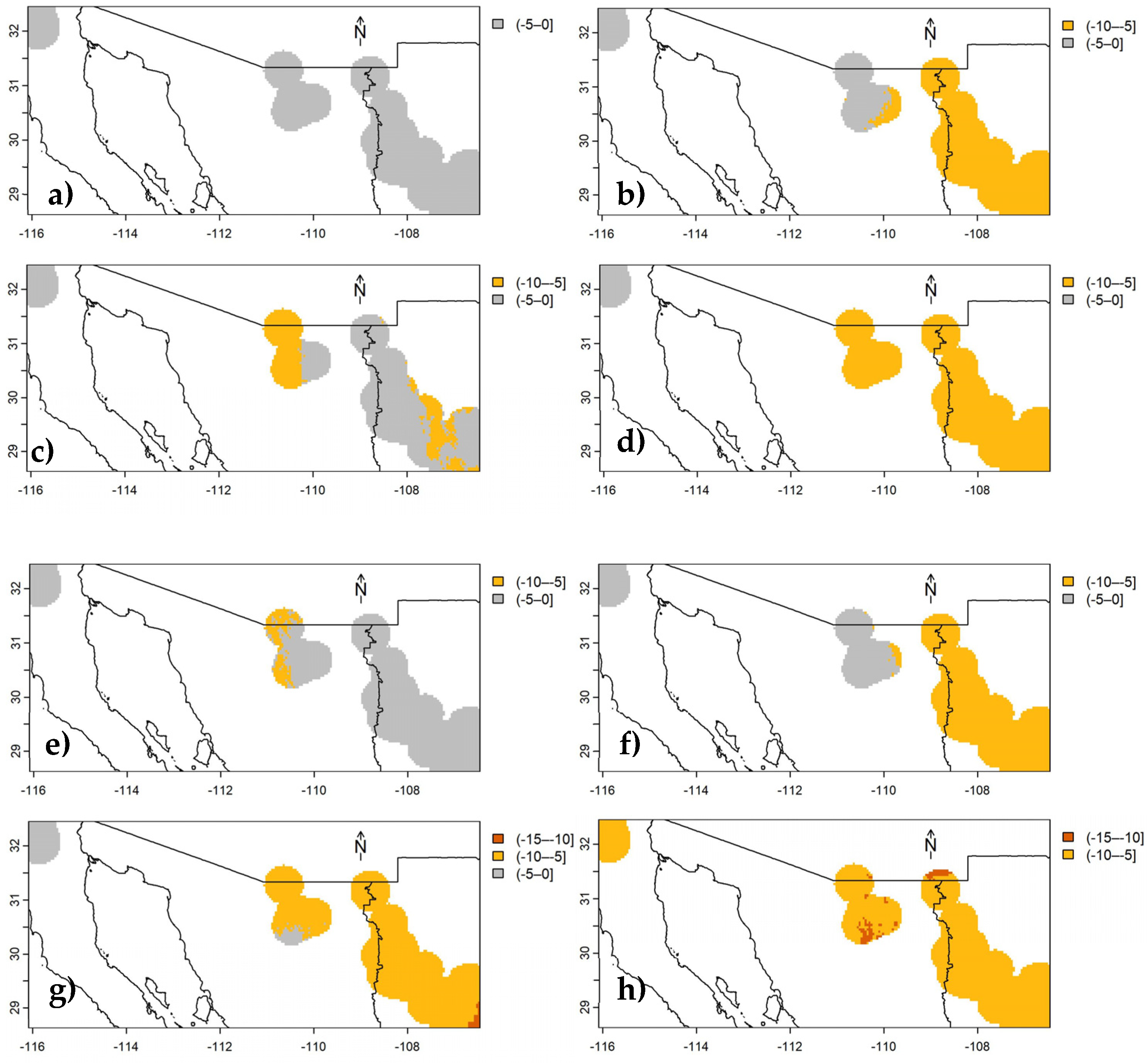
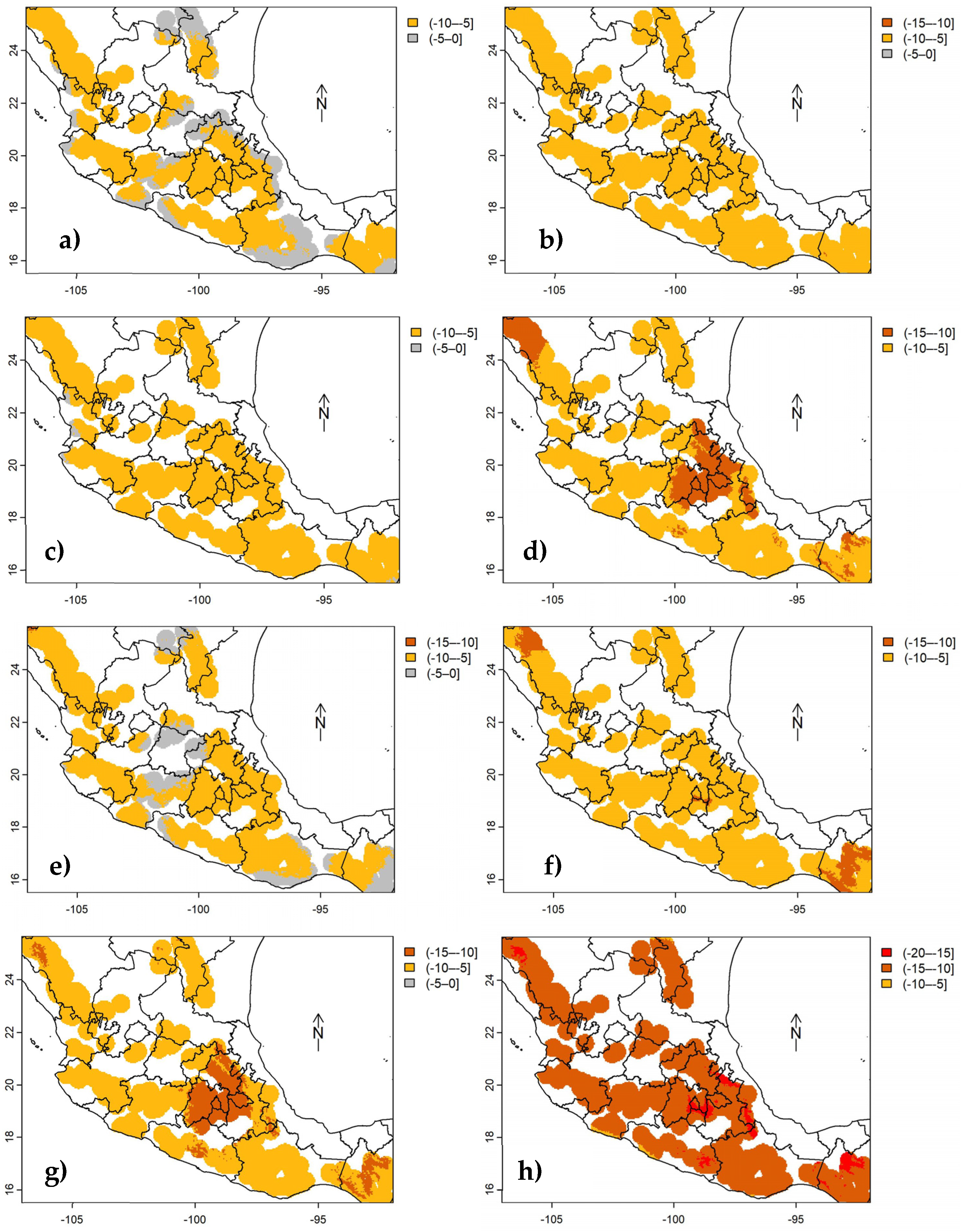
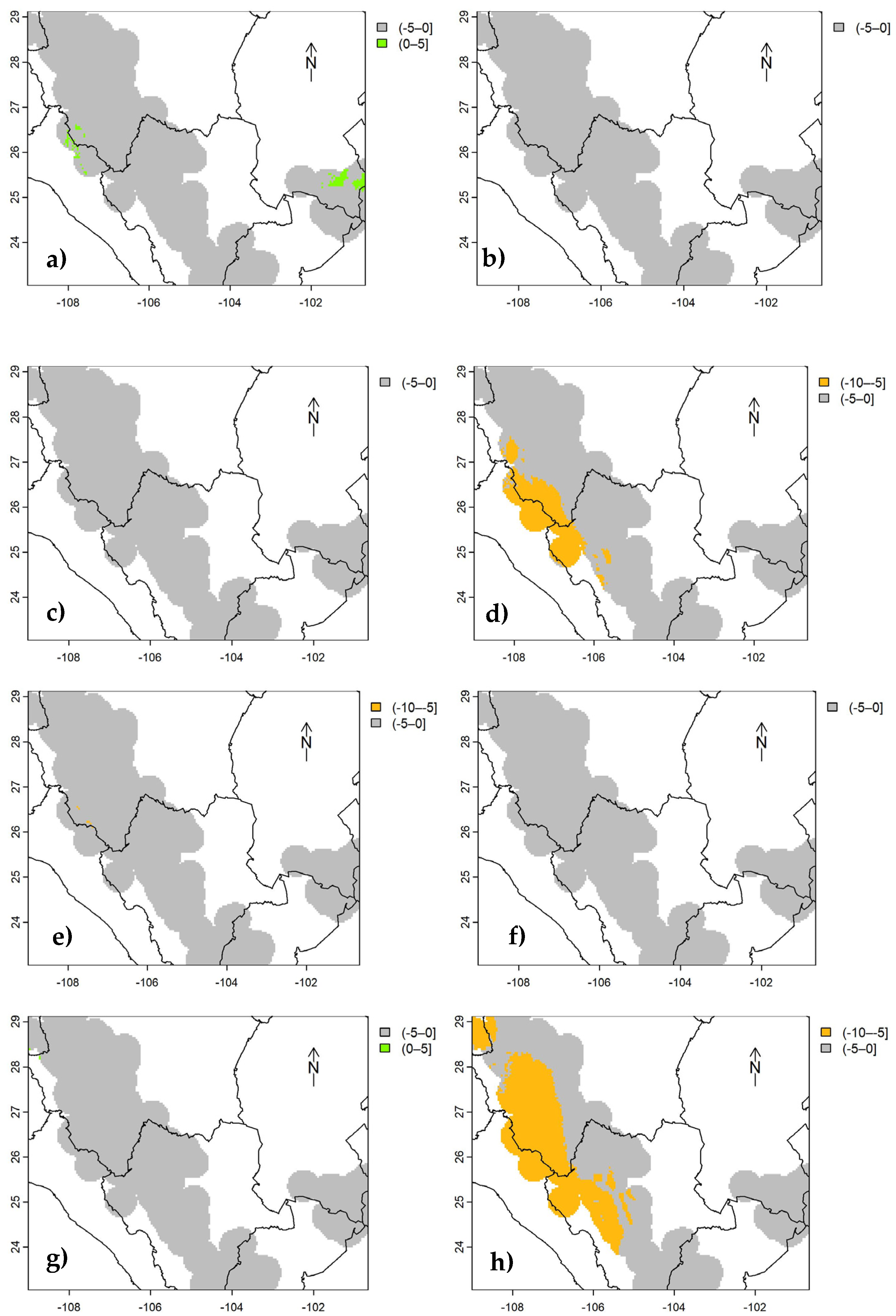
According to future predictions of cdAGB up to 2050 and 2070 (Figure 3, Figure 4 and Figure 5) using the bioclimatic model for each stratum (equations 1-3), under any climate scenario (RCP), only reductions in cdAGB are expected. Forests in stratum II (Figure 4a - Figure 4h, situated in the central and southern regions of the country) would be the most affected, with decreases ranging from -5 to -10 Mg ha-1, potentially up to -20 Mg C ha-1 by 2070, whereas those in stratum III (Figure 5a – Figure 5h, SMO) would experience lesser impacts ranging from 0 to -5 Mg C ha-1. The most significant losses of cdAGB are expected under RCP 8.5 and are anticipated to be greater by 2070.
Table 4. Number of pixels contained within the 40 km radius buffer around each sampling site of INFyS to differentiate changes in carbon density of aboveground live biomass in the conifer forests of Mexico under future climatic scenarios. Each pixel represents 0.98 x 0.98 km on each side.
Stratum Changes in
cdAGB
RCP 26 RCP 45 RCP 60 RCP 85
2050 2070 2050 2070 2050 2070 2050 2070
I (-20 – -15 | Preprints 121568 i001 ) 0 0 0 0 0 0 0 0
(-15 – -10 | Preprints 121568 i002 ) 0 0 0 0 0 35 0 107
(-10 – -5 | Preprints 121568 i003 ) 0 240 2361 2280 906 2885 3011 3180
(-5 – 0 | Preprints 121568 i004 ) 3287 3047 926 1007 2381 367 276 0
(0 – 5 | Preprints 121568 i005 ) 0 0 0 0 0 0 0 0
II (-20 – -15 | Preprints 121568 i001 ) 0 0 0 0 0 0 0 1148
(-15 – -10 | Preprints 121568 i002 ) 0 30 6 1526 0 3928 4796 22466
(-10 – -5 | Preprints 121568 i003 ) 17750 19473 23821 22317 23571 19912 19047 229
(-5 – 0 | Preprints 121568 i004 ) 6093 4340 16 0 272 3 0 0
(0 – 5 | Preprints 121568 i005 ) 0 0 0 0 0 0 0 0
III (-20 – -15 | Preprints 121568 i001 ) 0 0 0 0 0 0 0 0
(-15 – -10 | Preprints 121568 i002 ) 0 0 0 0 0 0 0 0
(-10 – -5 | Preprints 121568 i003 ) 0 6 0 0 0 0 1290 3281
(-5 – 0 | Preprints 121568 i004 ) 9680 9819 9825 9825 9825 9822 8535 6544
(0 – 5 | Preprints 121568 i005 ) 145 0 0 0 0 3 0 0
Where: Observed carbon density of aboveground live biomass (Mg C ha-1); RCP = Representative Concentration Pathways. The color of the box in column two corresponds to the color of the pixel in Figure 3, Figure 4 and Figure 5.

3.5. Evaluation of Climate Projections on Variables Predicting cdAGB

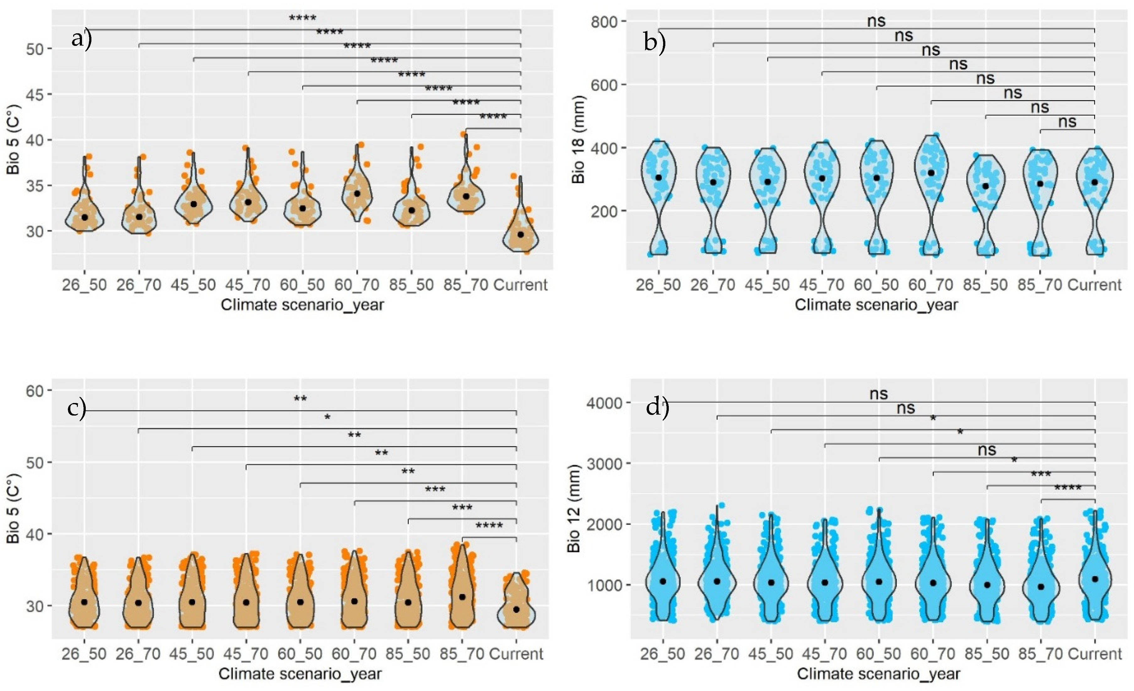
The Wilcoxon test provided sufficient evidence (p<0.0001) to reject the null hypothesis (H0) of equal medians between the current Bio and the same Bio under a future climate scenario. In all cases, the median of the estimated temperature Bios for 2050 and 2070, projected by three General Circulation Models (GCMs), in any climate scenario (RCP; left, Figure 6), will be higher than the current median (Table 2). Generally, the temperature is expected to increase by 2.66 °C (2050) and 3.36 °C (2070) compared to the present (Figure 6a, Figure 6c, and Figure 6e). The coniferous areas in stratum II are predicted to be vulnerable due to a likely increase of +2.7 °C by 2050, whereas the less vulnerable areas will be in stratum III (+2.5 °C).
Generally, the test demonstrated that in the coniferous forests of Mexico, precipitation levels in 2050 and 2070 could statistically be the same (p < 0.05) as those currently recorded in stratum I (Figure 6b). In stratum II, precipitation is projected to decrease (p < 0.0001) by 5.3% (2050) and 6.4% (2070) (Figure 6d), while in stratum III, it could either increase or decrease (Figure 6f). When analyzed individually (Current vs Bio-RCP-Year), significant differences exist only for precipitation variables (right, Figure 6), and not for temperature variables (left, Figure 6).
The uncertainty (represented by the standard error) estimated for cdAGB shown here (Figure 7), for the most critical scenario (RCP 85 | 2070), indicates that the standard error ranges from 2.5 Mg C ha-1 (stratum III) to 6 Mg C ha-1 (stratum II), well below the RMSE (Table 3) estimated with independent data. This uncertainty is similar in less critical climatic scenarios (RCP 26 | 2050; Figures not shown).

4. Discussion

The selection of cdAGB predictors through automated algorithms (stepwise, Machine Learning, neural networks, etc.) is generally efficient. These algorithms have been tested in natural forests [44,45], tropical rainforests [46], and even in plantations [19]. Although the variables selected by these algorithms are statistically significant, p<0.05 [36], the models generated here exhibited multicollinearity effects (VIF > 10), consequently, these models had to be evaluated to mitigate this effect and enhance the accuracy of the predictions.
Some authors [47] have used linear procedures (lm) for predicting NPP (Net Primary Production) in grasslands, with favorable results. We tested this technique; however, it was demonstrated that in this type of study, it is difficult to meet all the assumptions of a regression model ( ε i ~ N 0 , σ 2 , which is why the 'glm' procedure was ultimately employed, as has been done in such studies [2,9]. In addition to these procedures, Random Forest [8,48,49] and Bayesian models [20] have also been used for predicting AGB (Above-Ground Biomass) from temperature and precipitation variables.

4.1. Predictor Variables of Aboveground Biomass

In this study, the algorithms selected both temperature variables (Bio5 and Bio10) and precipitation variables (Bio12, Bio13, and Bio18) as the best predictors of cdAGB. Temperature variables were the most important in the model (contributing 8 to 10% to the pseudo R2) for strata I and II (Table 1, Figure 1a and Figure 1b), but not for stratum III. According to some authors [21,47], on a global scale, precipitation and temperature variables are the best predictors of AGB. Specifically, annual mean temperature (Bio1) and temperature of the warmest quarter (Bio10) are climatic variables associated with biomass distribution on broad scales. Metrics demonstrate that temperatures appear to be more important than precipitation variables [28].
It has been demonstrated that bioclimatic variables of temperature (Bio1 and Bio5) and precipitation (Bio12) are associated with the accumulation of AGB in forests [20], in boreal ecosystems [19], temperate seasonal ecosystems [18], tropical rainforests [50], and tropical seasonal ecosystems [4,5]. As can be noted, Bio5 and Bio12 (Appendix A) are good predictors of AGB across different types of ecosystems. For instance, a study conducted in the SMO (stratum II of this same study) indicates that average temperature (Bio1) is the most important predictor for AGB in temperate forests [24].
In Australian forests, encompassing 15 types of forests predominantly dominated by eucalypts [8], it has been demonstrated that climatic variables are better predictors of AGB than soil variables, with Bio 9 (Mean Temperature of Driest Quarter) being the most important variable. Regardless of the metrics, as in our study, temperature variables appear to be the most important for predicting AGB (Table 1).
However, the relationship between bioclimatic variables and AGB is entirely dependent on the type of ecosystem, the species, and the region of the world. For this reason, other authors emphasize that mean annual precipitation (MAP) has a relatively greater importance (0.19%) than mean annual temperature (MAT) (0.05%) for predicting AGB in Larix plantations in northern and northeastern China. Furthermore, its importance is also dependent on the model structure [19].
Continuing with the previous narrative, the relationship between precipitation and AGB can be complex, as different responses can be observed depending on the type of forest and climatic conditions. This variable significantly influences the accumulation of different components of AGB (branches, stems, roots, and needles) in conifer plantations. Therefore, it is important to consider it in predictive models and in the evaluation of the climate-forest relationship [12]. However, climatic variables such as temperature and precipitation together can improve AGB estimates [21]. In tropical forests [51], 13 predictor variables of AGB were used, including geographical, topographical, hydrological, soil, and even species-related variables (coverage), etc. They found that the relative influence of MAP on AGB is 37.6%, making it the most important, while MAT has a relative influence of less than 1%.

4.2. Correlation Between Bioclimatic Variables and Carbon Density

The correlation of cdAGB with temperature variables (Bio 5 and Bio 10) in temperate forests of Mexico is negative but positive with precipitation variables (Table 1). Similar findings were reported by [29], who observed a negative correlation (-0.46 > r < -0.63; -0.43 > r < -0.60) between the stem biomass of Larix gmelinii and Betula platyphylla with MAT. Likewise, other studies demonstrate that MAT is negatively correlated with AGB, either at the species level [12] or at the stand level [36].
Similar to this study, in temperate and dry forests, a positive correlation between cdAGB and MAP has been observed [26]. This same relationship is found in other studies; for instance, [29] discovered that MAP positively correlates with the stem biomass of Larix gmelinii (0.84 > r < 0.92) and Betula platyphylla (0.76 > r < 0.88). Additionally, [12] observed that MAP positively and significantly (p < 0.05) correlates with the AGB of Pinus koraiensis Siebold & Zucc., Larix olgensis A. Henry, and Pinus sylvestris var. mongolica Litv.
Furthermore, the study conducted by [28] reveals that on a global scale (> 6200 forests and 61 countries), MAT is positively correlated with foliage biomass, although the geographical patterns of correlation are inconsistent. [14] found that while temperature correlates positively in boreal forests, the opposite occurs in tropical forests. Studies conducted by [4] in boreal forests demonstrate that MAT can explain (R²) between 26% and 45% of carbon density and is positively correlated; whereas MAP can explain between 28% and 67% of carbon density (both aboveground and belowground); however, the correlation between these two variables is positive when precipitation is between 0 to 1000 mm, and negative when it exceeds 1000 mm.
In contrast to this study, in boreal and temperate forests, a positive relationship has been found between cdAGB and MAT [18], but a negative one in humid regions [26].

4.3. Predictive Capacity of Bioclimatic Models

Model validation is crucial for assessing the predictive capacity of a model based on new data. In reality, within this context (AGB-climatic predictors relationship), few studies undertake this process [19,47,48,52]. As known, when generating a model using the 'glm' procedure, statistics such as R2, RMSE, MAE, etc., are not computed. Upon validating our models, we were able to calculate these metrics and evaluate the predictive capacity of each model. We observed that bioclimatic variables can explain up to 22% of cdAGB in these types of forests (Table 3), a reasonably significant value at the eco-region level [4], but not at the species level [12,29], where variables can explain up to 84% of AGB at this scale.
In general, the 'cross-validation' technique has been the most commonly used to validate models for estimating AGB [19,36,52,53]; in this study, we used it along with three other techniques (Table 3). It is noteworthy that, when dealing with climatic predictors, these can explain around 20% (Table 3), whereas predicting AGB from predictors derived from vegetation indices, e.g., normalized difference vegetation index (NDVI), spectral information [52], or satellite optical images and unmanned aerial vehicles [53], can explain (R2) up to 80% of AGB. The inclusion of different predictor variables such as MAP, MAT, clay content, pH, dryness index, and stand age can explain up to 44.4% of cdAGB in temperate forests [4].
However, exclusive stand predictors (diameter at breast height, age, stand density) can explain up to 98% of the ABG variance [19]. The RMSE metric is entirely dependent on the units and scale of the dependent variables, which is why such distant differences are observed across studies.

4.4. Current and Future Projection of cdAGB

Under any climate scenario (RCP - year), our models predict losses in cdAGB ranging from 5 Mg C ha-1 (2050) to 20 Mg C ha-1 by 2070 (Figure 3, Figure 4 and Figure 5) in Mexico's coniferous forests. Globally, positive changes in Total Carbon Density (TCD) are projected for temperate forests, averaging 2.23 Mg C ha−1 (RCP 26, 45, and 85; 2050) and 1.99 Mg C ha−1 by 2070. Specifically for Mexico, these authors [4] predict changes of ±20 Mg C ha−1. It's important to note that, for the country, only two plots were considered in [4], whereas our study was conducted at a finer scale, generating models from n=48 to n=370 (Table 2).
A study conducted by [54] under various simulation scenarios, altering temperature and precipitation, in Yunnan Province, China, suggests that the combined effects of these variables are more complex than anticipated. They can result in both gains and losses (as observed in this study) in carbon sequestration across different forest types, attributed to decreased precipitation and increased temperature. Our study shows a decrease in cdAGB, primarily due to a temperature increase of 1 to 3°C and a precipitation decrease of approximately 10%. Nearly three decades ago [55], the vulnerability of Mexico's forests to climate change was assessed, revealing that under these conditions (+2°C and -10% precipitation), the area of humid and dry temperate forests would significantly decrease (to less than half of their current size).
In a study conducted in the Brazilian Atlantic Forest (AF) [56], it was found that in 34.7% of the existing forest fragments, AGB could increase, while in 2.6% it could decrease by the year 2100. Models predict an 8.5% increase in total carbon stock; additionally, 76.9% of AF would be suitable for a potential increase in AGB by 2100 under an RCP 4.5, solely due to climate change. This contrasts with findings here, possibly due to the type of forests and geographical location, but is similar to what was found by [36] in subtropical evergreen forests in China, showing a decrease in AGB by 2050-2070, varying according to different climate scenarios (RCP 2.6 > RCP 4.5 > RCP 6.0 > RCP 8.5).

5. Conclusions

The relationships between cdAGB and climate are more complex than they appear. Bioclimatic variables, especially those related to temperature, have proven to be significant predictors of cdAGB in the developed models and can explain up to 19% of cdAGB. Bio 5 (Max Temperature of Warmest Month) emerged as the most robust predictor. Predictions using bioclimatic models suggest that all strata of the country's coniferous forests, under any climate scenario (RCP - Year), will experience declines in cdAGB (in the absence of anthropogenic activities) by 2050 and 2070, particularly under the RCP 8.5 scenario. It is expected that forests in stratum II will be the most affected, with significant reductions that could reach up to -20 Mg C ha-1 by the year 2070. The temperature projected by the GCMs for 2050 and 2070 will be significantly higher than current levels, with increases of up to 3.55 °C in stratum I by 2070. Precipitation could remain unchanged in stratum I, decrease (-10%) in stratum II, and vary (±10%) in stratum III. These future climate projections are expected to lead to a redistribution of the cdAGB in Mexican forests. The conclusions suggest an urgent need for adaptation and mitigation strategies to conserve biodiversity and ecosystem services provided by conifer forests in Mexico. Forest management should consider not only biodiversity conservation but also the carbon storage capacity in these ecosystems.

Author Contributions

Conceptualization, J.M.G. and C.S.G.; methodology, J.M.G. and J.A.V.Q.; software, C.S.G.; validation, E.H.C.O., C.F.L. and A.F.; formal analysis, J.M.G.; investigation, F.P.P. and E.E.V.G.; resources, A.Z.G and L.S.D.; data curation, C.S.G., M.G.G. and A.F.; writing—original draft preparation, C.S.G.; writing—review and editing, E.H.C.O., A.Z.G. and E.E.V.G.; visualization, L.S.D. and M.G.G.; supervision, J.M.G; project administration, J.M.G. All authors have read and agreed to the published version of the manuscript.” Please turn to the CRediT taxonomy for the term explanation. Authorship must be limited to those who have contributed substantially to the work reported.

Funding

“This research was funded by AUTONOMOUS AGRARIAN UNIVERSITY ANTONIO NARRO, grant number 38111425103001-2185”.

Data Availability Statement

We encourage all authors of articles published in MDPI journals to share their research data. In this section, please provide details regarding where data supporting reported results can be found, including links to publicly archived datasets analyzed or generated during the study. Where no new data were created, or where data is unavailable due to privacy or ethical restrictions, a statement is still required. Suggested Data Availability Statements are available in section “MDPI Research Data Policies” at https://www.mdpi.com/ethics.

Acknowledgments

The authors are grateful to the AUTONOMOUS AGRARIAN UNIVERSITY ANTONIO NARRO, for funding all stages of this study through Project No 38111425103001-2185.

Conflicts of Interest

The authors declare no conflicts of interest. The funders had no role in the design of the study; in the collection, analyses, or interpretation of data; in the writing of the manuscript; or in the decision to publish the results.

Appendix A. Bioclimatic Variables

Variable Description Units Scale
Bio 1 Annual Mean Temperature °C Annual
Bio 2 Mean Diurnal Range (max temp - min temp) °C Monthly
Bio 3 Isothermality (Bio02/Bio07) (×100) % Annual
Bio 4 Temperature Seasonality (standard deviation × 100) % Annual
Bio 05 Max Temperature of Warmest Month °C Monthly
Bio 06 Min Temperature of Coldest Month °C Monthly
Bio 07 Temperature Annual Range (Bio5–Bio6) °C Annual
Bio 08 Mean Temperature of Wettest Quarter °C Quarterly
Bio 09 Mean Temperature of Driest Quarter °C Quarterly
Bio 10 Mean Temperature of Warmest Quarter °C Quarterly
Bio 11 Mean Temperature of Coldest Quarter °C Quarterly
Bio 12 Annual Precipitation mm Annual
Bio 13 Precipitation of Wettest Month mm Monthly
Bio 14 Precipitation of Driest Month mm Monthly
Bio 15 Precipitation Seasonality (Coefficient of variation) % Quarterly
Bio 16 Precipitation of Wettest Quarter mm Quarterly
Bio 17 Precipitation of Driest Quarter mm Quarterly
Bio 18 Precipitation of Warmest Quarter mm Quarterly
Bio 19 Precipitation of Coldest Quarter mm Quarterly

References

  1. FAO, 2022. El Estado de Los Bosques Del Mundo 2022; FAO, 2022; ISBN 978-92-5-136479-6.
  2. Arasa-Gisbert, R.; Vayreda, J.; Román-Cuesta, R.M.; Villela, S.A.; Mayorga, R.; Retana, J. Forest Diversity Plays a Key Role in Determining the Stand Carbon Stocks of Mexican Forests. For Ecol Manage 2018, 415–416, 160–171. [CrossRef]
  3. Rodríguez-Veiga, P.; Saatchi, S.; Tansey, K.; Balzter, H. Magnitude, Spatial Distribution and Uncertainty of Forest Biomass Stocks in Mexico. Remote Sens Environ 2016, 183, 265–281. [CrossRef]
  4. Guo, Y.; Peng, C.; Trancoso, R.; Zhu, Q.; Zhou, X. Stand Carbon Density Drivers and Changes under Future Climate Scenarios across Global Forests. For Ecol Manage 2019, 449. [CrossRef]
  5. Ma, Y.; Eziz, A.; Halik, Ü.; Abliz, A.; Kurban, A. Precipitation and Temperature Influence the Relationship between Stand Structural Characteristics and Aboveground Biomass of Forests—A Meta-Analysis. Forests 2023, 14.
  6. IPCC, 2021. In Climate Change 2021 – The Physical Science Basis; Cambridge University Press, 2021; pp. 3–32.
  7. 2024; 7. MEXICO CLIMATE RISK COUNTRY PROFILE; 2024;
  8. Bennett, A.C.; Penman, T.D.; Arndt, S.K.; Roxburgh, S.H.; Bennett, L.T. Climate More Important than Soils for Predicting Forest Biomass at the Continental Scale. Ecography 2020, 43, 1692–1705. [CrossRef]
  9. Cysneiros, V.C.; Coelho de Souza, F.; Gaui, T.D.; Pelissari, A.L.; Orso, G.A.; Machado, S. do A.; de Carvalho, D.C.; Silveira-Filho, T.B. Integrating Climate, Soil and Stand Structure into Allometric Models: An Approach of Site-Effects on Tree Allometry in Atlantic Forest. Ecol Indic 2021, 127. [CrossRef]
  10. Gao, J.; Zhao, P.; Shen, W.; Rao, X.; Hu, Y. Physiological Homeostasis and Morphological Plasticity of Two Tree Species Subjected to Precipitation Seasonal Distribution Changes. Perspect Plant Ecol Evol Syst 2017, 25, 1–19. [CrossRef]
  11. Yuan, J.; Yan, Q.; Wang, J.; Xie, J.; Li, R. Different Responses of Growth and Physiology to Warming and Reduced Precipitation of Two Co-Existing Seedlings in a Temperate Secondary Forest. Front Plant Sci 2022, 13. [CrossRef]
  12. Xin, S.; Wang, J.; Mahardika, S.B.; Jiang, L. Sensitivity of Stand-Level Biomass to Climate for Three Conifer Plantations in Northeast China. Forests 2022, 13. [CrossRef]
  13. Eamus, D. How Does Ecosystem Water Balance Affect Net Primary Productivity of Woody Ecosystems? Functional Plant Biology 2003, 30, 187–205. [CrossRef]
  14. Liu, Y.; Yu, G.; Wang, Q.; Zhang, Y. How Temperature, Precipitation and Stand Age Control the Biomass Carbon Density of Global Mature Forests. Global Ecology and Biogeography 2014, 23, 323–333. [CrossRef]
  15. Sim-Hee Han 2012.
  16. Devi, V.; Kaur, A.; Sethi, M.; Avinash, G. Perspective Chapter: Effect of Low-Temperature Stress on Plant Performance and Adaptation to Temperature Change;
  17. Pan, Y.; Birdsey, R.A.; Phillips, O.L.; Jackson, R.B. The Structure, Distribution, and Biomass of the World’s Forests. Annu Rev Ecol Evol Syst 2013, 44, 593–622.
  18. Keith, H.; Mackey, B.G.; Lindenmayer, D.B. Re-Evaluation of Forest Biomass Carbon Stocks and Lessons from the World’s Most Carbon-Dense Forests. Proc Natl Acad Sci U S A 2009, 106, 11635–11640. [CrossRef]
  19. He, X.; Lei, X.; Zeng, W.; Feng, L.; Zhou, C.; Wu, B. Quantifying the Effects of Stand and Climate Variables on Biomass of Larch Plantations Using Random Forests and National Forest Inventory Data in North and Northeast China. Sustainability (Switzerland) 2022, 14. [CrossRef]
  20. Chen, X.; Luo, M.; Larjavaara, M. Effects of Climate and Plant Functional Types on Forest Above-Ground Biomass Accumulation. Carbon Balance Manag 2023, 18. [CrossRef]
  21. Dai, L.; Ke, X.; Guo, X.; Du, Y.; Zhang, F.; Li, Y.; Li, Q.; Lin, L.; Peng, C.; Shu, K.; et al. Responses of Biomass Allocation across Two Vegetation Types to Climate Fluctuations in the Northern Qinghai–Tibet Plateau. Ecol Evol 2019, 9, 6105–6115. [CrossRef]
  22. Khan, D.; Muneer, M.A.; Nisa, Z.U.; Shah, S.; Amir, M.; Saeed, S.; Uddin, S.; Munir, M.Z.; Lushuang, G.; Huang, H. Effect of Climatic Factors on Stem Biomass and Carbon Stock of Larix Gmelinii and Betula Platyphylla in Daxing’anling Mountain of Inner Mongolia, China. Advances in Meteorology 2019, 2019. [CrossRef]
  23. David, H.C.; de Araújo, E.J.G.; Morais, V.A.; Scolforo, J.R.S.; Marques, J.M.; Péllico Netto, S.; MacFarlane, D.W. Carbon Stock Classification for Tropical Forests in Brazil: Understanding the Effect of Stand and Climate Variables. For Ecol Manage 2017, 404, 241–250. [CrossRef]
  24. López-Serrano, P.M.; Domínguez, J.L.C.; Corral-Rivas, J.J.; Jiménez, E.; López-Sánchez, C.A.; Vega-Nieva, D.J. Modeling of Aboveground Biomass with Landsat 8 Oli and Machine Learning in Temperate Forests. Forests 2020, 11. [CrossRef]
  25. Rezashobairi, S.; Lin, H.; Usoltsev, V.; Osmirko, A.; Tsepordey, I.; Ye, Z.; Anees, S. A Comparative Pattern for Populus Spp. and Betula Spp. Stand Biomass in Eurasian Climate Gradients. Croatian Journal of Forest Engineering 2022, 43, 457–467. [CrossRef]
  26. Stegen, J.C.; Swenson, N.G.; Enquist, B.J.; White, E.P.; Phillips, O.L.; Jørgensen, P.M.; Weiser, M.D.; Monteagudo Mendoza, A.; Núñez Vargas, P. Variation in Above-Ground Forest Biomass across Broad Climatic Gradients. Global Ecology and Biogeography 2011, 20, 744–754. [CrossRef]
  27. Girón-Gutiérrez, D.; Méndez-González, J.; Osorno-Sánchez, T.G.; Cerano-Paredes, J.; Soto-Correa, J.C.; Cambrón-Sandoval, V.H. Climate as a Driver of Aboveground Biomass Density Variation: A Study of Ten Pine Species in Mexico. Forests 2024, 15, 1160. [CrossRef]
  28. Reich, P.B.; Luo, Y.; Bradford, J.B.; Poorter, H.; Perry, C.H.; Oleksyn, J. Temperature Drives Global Patterns in Forest Biomass Distribution in Leaves, Stems, and Roots. Proc Natl Acad Sci U S A 2014, 111, 13721–13726. [CrossRef]
  29. Khan, D.; Muneer, M.A.; Nisa, Z.U.; Shah, S.; Amir, M.; Saeed, S.; Uddin, S.; Munir, M.Z.; Lushuang, G.; Huang, H. Effect of Climatic Factors on Stem Biomass and Carbon Stock of Larix Gmelinii and Betula Platyphylla in Daxing’anling Mountain of Inner Mongolia, China. Advances in Meteorology 2019, 2019. [CrossRef]
  30. Gernandt, D.S.; Pérez-De La Rosa, J.A. Biodiversity of Pinophyta (Conifers) in Mexico. Rev Mex Biodivers 2014, 85. [CrossRef]
  31. Rzedowski, J.; Huerta, L. Vegetación de México; 2006;
  32. Granados-Sánchez, D.; López-Ríos, G.F.; Hernández-García, M.A. Sistema de Información Científica;
  33. Challenger, A. Utilización y Conservación de Los Ecosistemas Terrestres de México: Pasado, Presente y Futuro. 1998.
  34. Penman, J.; Carruthers, I.; López, C. Capítulo 1: Panorama General AUTORES Y EDITORES REVISORES Autores Principales Coordinadores Editores Revisores;
  35. Fick, S.E.; Hijmans, R.J. WorldClim 2: New 1-km Spatial Resolution Climate Surfaces for Global Land Areas. International Journal of Climatology 2017, 37, 4302–4315. [CrossRef]
  36. Li, Y.; Li, M.; Wang, Y. Forest Aboveground Biomass Estimation and Response to Climate Change Based on Remote Sensing Data. Sustainability (Switzerland) 2022, 14. [CrossRef]
  37. Hijmans, R.J. Raster: Geographic Data Analysis and Modeling [Data Set]. En CRAN: Contributed Pa-Ckages. The R Foundation. 2010.
  38. Lê, S.; Josse, J.; Rennes, A.; Husson, F. FactoMineR: An R Package for Multivariate Analysis; 2008; Vol. 25;.
  39. Bivand, R., G.-R.V., & P.E. GeoStratR: Tools for Simple Stratification of Spatial Patterns. 2022.
  40. Kuhn, M. Journal of Statistical Software Building Predictive Models in R Using the Caret Package; 2008;
  41. Grömping, U. Relative Importance for Linear Regression in R: The Package Relaimpo; 2006; Vol. 17;.
  42. IPCC, 2013 Climate Change 2013: The Physical Science Basis. Contribution of Working Group I to the Fifth Assessment Report of the Intergovernmental Panel on Climate Change [Stocker, T.F., D. Qin, G.-K. Plattner, M. Tignor, S.K. Allen, J. Boschung, A. Nauels, Y. Xia, V. Bex and P.M. Midgley (Eds.)]. 2013.
  43. R Core Team. R: A Language and Environment for Statistical Computing; R Foundation for Statistical Computing. 2024.
  44. Luo, M.; Wang, Y.; Xie, Y.; Zhou, L.; Qiao, J.; Qiu, S.; Sun, Y. Combination of Feature Selection and Catboost for Prediction: The First Application to the Estimation of Aboveground Biomass. Forests 2021, 12, 1–22. [CrossRef]
  45. Bjork, S.; Anfinsen, S.N.; Naesset, E.; Gobakken, T.; Zahabu, E. On the Potential of Sequential and Nonsequential Regression Models for Sentinel-1-Based Biomass Prediction in Tanzanian Miombo Forests. IEEE J Sel Top Appl Earth Obs Remote Sens 2022, 15, 4612–4639. [CrossRef]
  46. Ortiz-Reyes, A.D.; Valdez-Lazalde, J.R.; Ángeles-Pérez, G.; de los Santos-Posadas, H.M.; Schneider, L.; Aguirre-Salado, C.A.; Peduzzi, A. Synergy of Landsat, Climate and LiDAR Data for Aboveground Biomass Mapping in Medium-Stature Tropical Forests of the Yucatan Peninsula, Mexico. Revista Chapingo, Serie Ciencias Forestales y del Ambiente 2021, 27, 383–400. [CrossRef]
  47. Zhang, H.; Feng, Z.; Shen, C.; Li, Y.; Feng, Z.; Zeng, W.; Huang, G. Relationship between the Geographical Environment and the Forest Carbon Sink Capacity in China Based on an Individual-Tree Growth-Rate Model. Ecol Indic 2022, 138. [CrossRef]
  48. Cartus, O.; Kellndorfer, J.; Walker, W.; Franco, C.; Bishop, J.; Santos, L.; Fuentes, J.M.M. A National, Detailed Map of Forest Aboveground Carbon Stocks in Mexico. Remote Sens (Basel) 2014, 6, 5559–5588. [CrossRef]
  49. Yan, M.; Xia, Y.; Yang, X.; Wu, X.; Yang, M.; Wang, C.; Hou, Y.; Wang, D. Biomass Estimation of Subtropical Arboreal Forest at Single Tree Scale Based on Feature Fusion of Airborne LiDAR Data and Aerial Images. Sustainability (Switzerland) 2023, 15. [CrossRef]
  50. Chen, L.; Ren, C.; Zhang, B.; Wang, Z.; Xi, Y. Estimation of Forest Above-Ground Biomass by Geographically Weighted Regression and Machine Learning with Sentinel Imagery. Forests 2018, 9. [CrossRef]
  51. Adhikari, H.; Heiskanen, J.; Siljander, M.; Maeda, E.; Heikinheimo, V.; Pellikka, P.K.E. Determinants of Aboveground Biomass across an Afromontane Landscape Mosaic in Kenya. Remote Sens (Basel) 2017, 9.
  52. Opelele, O.M.; Yu, Y.; Fan, W.; Chen, C.; Kachaka, S.K. Biomass Estimation Based on Multilinear Regression and Machine Learning Algorithms in the Mayombe Tropical Forest, in the Democratic Republic of Congo. Appl Ecol Environ Res 2021, 19, 359–377. [CrossRef]
  53. Wang, Z.; Yi, L.; Xu, W.; Zheng, X.; Xiong, S.; Bao, A. Integration of UAV and GF-2 Optical Data for Estimating Aboveground Biomass in Spruce Plantations in Qinghai, China. Sustainability (Switzerland) 2023, 15. [CrossRef]
  54. Zhou, R.; Zhang, Y.; Peng, M.; Jin, Y.; Song, Q. Effects of Climate Change on the Carbon Sequestration Potential of Forest Vegetation in Yunnan Province, Southwest China. Forests 2022, 13. [CrossRef]
  55. Villers-Ruiz, L.; Trejo-Vazquez, I. CLIMATE RESEARCH Clim Res Assessment of the Vulnerability of Forest Ecosystems to Climate Change in Mexico; 1997; Vol. 9;.
  56. Ferreira, I.J.M.; Campanharo, W.A.; Fonseca, M.G.; Escada, M.I.S.; Nascimento, M.T.; Villela, D.M.; Brancalion, P.; Magnago, L.F.S.; Anderson, L.O.; Nagy, L.; et al. Potential Aboveground Biomass Increase in Brazilian Atlantic Forest Fragments with Climate Change. Glob Chang Biol 2023, 29, 3098–3113. [CrossRef]
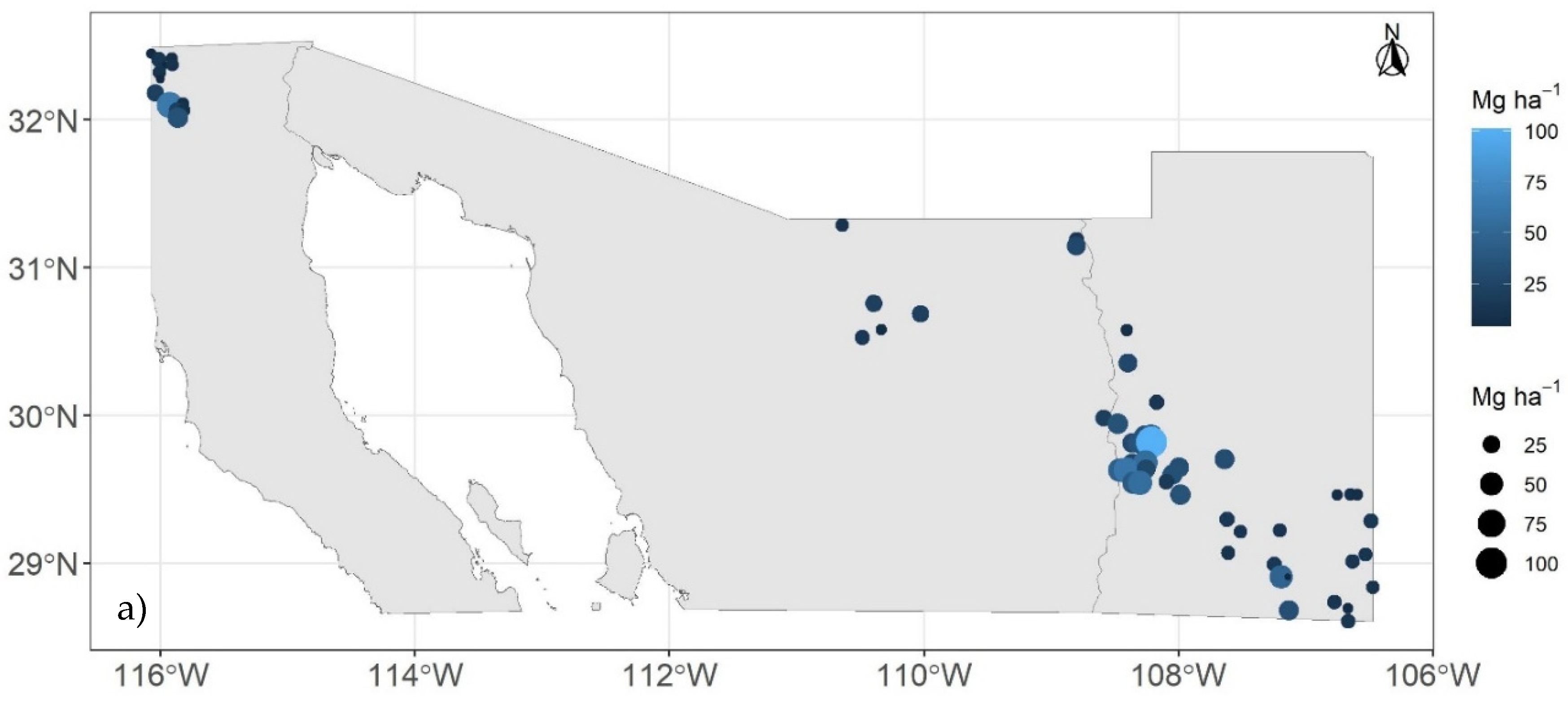
Figure 1. Distribution of sites from the National Forest and Soil Inventory (2009 - 2012): stratum I (a), stratum II (b), and stratum III (c). The size of the circles and the color gradient indicate the values of carbon density in the aboveground live biomass (Mg C ha-1).
Preprints 121568 g001aPreprints 121568 g001b
Figure 2. Prediction of current carbon density of aboveground live biomass in Mexican conifer forests through bioclimatic models: stratum I (a), stratum II (b), stratum III (c). Circle size and color gradient indicate values of carbon density of aboveground live biomass (Mg C ha-1).
Preprints 121568 g002
Figure 3. Changes in carbon density of aboveground live biomass in Mexican conifer forests under RCP 2.6 to 8.5 scenarios (from left to right), for the years 2050 (top) and 2070 (bottom), in stratum I. Colored areas represent 40 km radius buffers around each INFyS site; uncolored areas correspond to other vegetation types different from conifer forests.
Preprints 121568 g003
Figure 4. Changes in carbon density of aboveground live biomass in Mexican conifer forests under RCP 2.6 to 8.5 scenarios (from left to right), for the years 2050 (top) and 2070 (bottom), in stratum II. Colored areas represent 40 km radius buffers around each INFyS site; uncolored areas correspond to other vegetation types different from conifer forests.
Preprints 121568 g004
Figure 5. Changes in carbon density of aboveground live biomass in Mexican conifer forests under RCP 2.6 to 8.5 scenarios (from left to right), for the years 2050 (top) and 2070 (bottom), in stratum III. Colored areas represent 40 km radius buffers around each INFyS site; uncolored areas correspond to other vegetation types different from conifer forests.
Preprints 121568 g005
Figure 6. Wilcoxon test for comparing medians of the current variable with each climate scenario, in stratum I (a-b), II (b-c), and III (e-f). Bio 05: Max Temperature of Warmest Month (°C); Bio 10: Mean Temperature of Warmest Quarter (°C); Bio 12: Annual Precipitation (mm); Bio 13: Precipitation of Wettest Month (mm); Bio 18: Precipitation of Warmest Quarter (mm). Significance levels: NS (Not significant), * (Significant at 0.05%), ** (Significant at 1%), *** (Significant at 0.1%), **** (Significant at 0.01%).
Preprints 121568 g006aPreprints 121568 g006b
Figure 7. Estimated uncertainty (standard error) of carbon density of aboveground live biomass in Mexican conifer forests, for strata I (a), II (b), and III (c) under RCP 85 and for the year 2070.
Preprints 121568 g007
Table 1. Regression coefficients for the prediction of the carbon density of aboveground live biomass by stratum in the coniferous forests of Mexico.
Stratum Coefficient Estimate 2.5 97.5 Std. T Pr Residual VIF Imp.(%)
Err value (>|t|) deviance
I β0 (intercept) 64.8332 22.7606 97.3943 23.2221 2.79 0.00772 ** 13.246
(n=48) β1 (Bio 5) -0.1897 -0.2932 -0.0544 0.0737 -2.57 0.01355 * 1.02 10.33
β2 (Bio 18) 0.0586 0.0337 0.0829 0.0123 4.77 2.02e-05 *** 1.02 8.74
II β0 (intercept) 87.6362 66.3661 108.9076 10.4558 8.38 1.22e-15 *** 172.17
(n=360) β1 (Bio 5) -0.2572 -0.3296 -0.1841 0.0376 -6.84 3.37e-11 *** 1.03 8.04
β2 (Bio 12) 0.0190 0.0106 0.0272 0.0037 5.12 4.91e-07 *** 1.03 3.35
III β0 (intercept) 26.6379 12.3682 40.4383 8.4994 3.13 0.00186 ** 132.39
(n=370) β1 (Bio 10) -0.0959 -0.1571 -0.0293 0.0391 -2.45 0.01461 * 1.16 3.28
β2 (Bio 13) 0.0933 0.0708 0.1160 0.0135 6.93 1.8e-11 *** 1.16 14.95
Where: β0, β1 and β2: are the regression coefficients; 2.5 and 97.5: 95% confidence intervals of the regression coefficients; Std. Err: standard error of the regression coefficients; Pr (>|t|): The probability of obtaining a t-value more extreme than the observed one, assuming that the null hypothesis is true. VIF: variance inflation factor; Imp = importance value of the variables. Bio 05: Max Temperature of Warmest Month (°C); Bio 10: Mean Temperature of Warmest Quarter (°C); Bio 12: Annual Precipitation (mm); Bio 13: Precipitation of Wettest Month (mm); Bio 18: Precipitation of Warmest Quarter (mm). Statistical significance: "* p < 0.05": Significant; "** p < 0.01": Highly significant; "*** p < 0.001": Very highly significant.
Table 2. Descriptive statistics of the observed carbon density of aboveground live biomass and its predictors (1950-2000 period) in the coniferous forests of Mexico.
Stratum Parameter n Min P25 Mean Median P75 Max SD CV Shapiro Anderson
p-value p-value
I cdAGB 48 4.23 11.54 23.14 16.23 33.35 62.05 15.04 65 0.0001 0.0001
Bio 5 27.7 28.7 29.97 29.6 30.75 36 1.76 5.89 0.0001 0.0001
Bio 18 62 223 256.89 290 330.5 397 101.66 39.57 0.0001 0.0001
II cdAGB 360 4.46 19.87 42.57 34.35 54.75 179.69 33.01 77.54 0.0001 0.0001
Bio 5 17.5 22.78 25.72 25.3 28.7 34.6 3.93 15.28 0.0001 0.0001
Bio 12 426 895.25 1109.42 1092 1314.25 2216 367.25 33.1 0.0001 0.0001
III cdAGB 370 3.15 12.76 26.26 23.24 35.98 92.92 16.56 63.05 0.0001 0.0001
Bio 10 14.7 17.4 18.55 18.3 19.4 26.3 1.74 9.39 0.0001 0.0001
Bio13 53 154 184.03 181 219 357 52.54 28.55 0.0001 0.0001
Where: cdAGB: carbon density of aboveground live biomass (Mg C ha-1); Bio 5: Max Temperature of Warmest Month (°C); Bio18: Precipitation of Warmest Quarter (mm); Bio12: Annual Precipitation (mm); Bio10: Mean Temperature of Warmest Quarter (°C); Bio13: Precipitation of Wettest Month (mm); n = number of sites in the stratum; Min: minimum value; P25 and P75: 25th and 75th percentiles; Max: maximum value; SD: standard deviation; CV: coefficient of variation (%).
Table 3. Validation of bioclimatic regression models for predicting carbon density of aboveground live biomass in coniferous forests in Mexico.
Stratum Method Set n Pseudo R2 RMSE MAE
Training 48
I LOOCV Validation 12 0.031 38.319 30.806
CV Validation 12 0.177 29.908 29.379
RCV Validation 12 0.177 31.949 31.272
II Bootstrap Validation 12 0.316 42.426 34.457
Training 360
LOOCV Validation 90 0.128 29.938 21.789
CV Validation 90 0.249 28.493 21.720
RCV Validation 90 0.246 28.620 21.685
Bootstrap Validation 90 0.150 30.107 22.302
III Training 370
LOOCV Validation 92 0.153 13.887 10.699
CV Validation 92 0.231 13.181 10.543
RCV Validation 92 0.238 13.330 10.600
Bootstrap Validation 92 0.192 14.175 10.986
Where: LOOCV: Leave-One-Out Cross-Validation; CV: Cross-Validation; RCV: Repeated Cross-Validation; n: sample size; R2: Coefficient of Determination; RMSE: Root Mean Square Error; MAE: Mean Absolute Error.
Disclaimer/Publisher’s Note: The statements, opinions and data contained in all publications are solely those of the individual author(s) and contributor(s) and not of MDPI and/or the editor(s). MDPI and/or the editor(s) disclaim responsibility for any injury to people or property resulting from any ideas, methods, instructions or products referred to in the content.
Copyright: This open access article is published under a Creative Commons CC BY 4.0 license, which permit the free download, distribution, and reuse, provided that the author and preprint are cited in any reuse.
Prerpints.org logo

Preprints.org is a free preprint server supported by MDPI in Basel, Switzerland.

Subscribe

© 2024 MDPI (Basel, Switzerland) unless otherwise stated