1. Introduction
Advances in technology and industry have helped mankind to increase the quality of life and life expectancy. This includes the delegation of laborious processes traditionally performed by hand to machines, which can perform these tasks more efficiently. However, it has also brought with it several well-known problems such as overexploitation and non-rational use of the earth’s natural resources. For Smarter Agriculture, demonstrating how the accessibility of tools, methods, and software, as well as the increasing openness of heterogeneous data sources (the open data wave), will encourage more academic research, public sector initiatives, and entrepreneurial initiatives in the agricultural sector [
1].
Plants become more prone to disease due to the large number of pathogens surrounding them. Pest and disease attacks are significative causes of reduced crop yields. Accurate and timely prediction of plant diseases helps to apply appropriate prevention and protection measures. Therefore, it helps to improve yield quality and increase crop productivity. Plant diseases are detected by various symptoms such as lesions, color changes, damaged leaves, stem damage, abnormal growth of stem, leaf, bud, florm and/or root, etc. In addition, leaves show symptoms such as spotting, dryness, premature drooping, etc., as an indicator of disease [
2].
Early solutions to computer vision tasks relied on traditional machine learning methods, i.e. manual feature-based methods [
3].
Similarly, early classification of plant diseases will help farmers use the best strategies to combat them. Using sensors, machine vision, AI models, and robots allows harvesting processes to be performed on behalf of workers with greater accuracy and speed. In addition, it helps to reduce crop wastage in the field which is experienced with the traditional harvesting method. Finally, the process of early detection of pests in plants helps to reduce economic loss due to the execution of prevention protocols when pests are detected at an early stage [
4].
We will list some papers that were reviewed during the research related to precision agriculture and crop pest detection. It is essential to understand that in this list some papers use neural networks because these papers provide different ways to handle the problem.
In [
5] proposed a recommendation system for farmers in real-time using sensors, IoT devices, and machine learning algorithms in addition the proposed architecture consists of 3 layers which are the data acquisition layer which is the first layer that is responsible for the continuous monitoring of water level, temperature, humidity, light intensity, and rainfall level, The data processing layer helps the data processing through a master node that receives information from the previous layer and sends it via wifi to the cloud and finally the visualization and analysis layer that preprocesses the data in the cloud server with XGBoost and sends the recommendations in real time where the optimization of the system in the cloud is concluded.
In [
6] proposed analysis for the detection of pests in plants using images and implementing two machine learning models which are support vector machine and Alex-net deeplearning where 3 important factors of the architecture are taken into consideration which are the computational power and the amount of input data having as a result
% of the pressure in SVM and in the neural network 97% of accuracy.
In [
7] conducted a study on the population fluctuations of citrus with the whitefly in a 4-hectare orchard in the citrus region of Chlef, first by sampling the population of the pest from July 2013 to June 2014 every two weeks, then entering the stage of infestation rate where the townsmen-heuberger formula calculates it, the following stages are the rate of parasitism by C. noaki, phenology of the orange tree in relation to the climatic data and finally the statistical analysis. Naoki, phenology of the orange tree in relation to the climatic data, and finally the statistical analysis. It is worth mentioning that these stages go through the parasite count per 1cm square area, the growth cycles of the orange tree, and the data analyzed by the ANOVA and general linear model (GLM) methods, having as results the temporal variation of the pest as the evolution of the abundance indexes where 3 abundance peaks of the study are presented and it shows the periods of fluctuation of the pest.
In [
8] proposed a model for the prediction of apple orchard disease in apple orchards where it is carried out in the Kashmir valley and also makes use of different methods for data analysis, machine learning algorithms such as linear regression and IoT systems using WSN network by adding sensors and using ZigBee and finally tests the farmers, as a result, examines the different challenges that have to overcome the incorporation of technology in the agricultural area.
In [
9], a methodology was developed for the detection of pests and diseases in citrus, using Self-Attention YOLOV8, with hyperspectral and multispectral imaging techniques to analyze different wavelengths with a focus on artificial vision technology taking into account characteristics such as texture, color, and shape. However, in this work, they use convolutional neural networks such as YOLOV8 to detect pests, which require a large variety of data for training, and it is more difficult to understand how they reach these conclusions compared to more transparent conventional methods.
In [
10], a review is conducted for pest detection and classification using deep learning techniques. This study reviews different neural network models such as CNNs and their application in agriculture to improve the accuracy of disease identification. It also compares approaches with conventional methods and highlights the advantages and limitations of deep learning in this emerging field.
In [
11], a methodology for early detection of crop pests using CNN-type artificial neural networks was developed. This methodology considers several relevant attributes of plant images. Among the main results, the high accuracy in the identification of pests in the early stages of infestation is highlighted. However, the paper also discusses some limitations and areas for future improvements in the approach used.
In [
12] presents an approach for disease detection in citrus fruits and leaves using DenseNet, a deep convolutional neural network architecture. DenseNet takes advantage of dense connectivity between layers to improve detection efficiency and accuracy. The study demonstrates that this model is effective in identifying multiple citrus diseases, outperforming other techniques in terms of accuracy and speed, and offering a valuable tool for precision agriculture.
The aim of this article is to study a new proposal for machine learning and image processing techniques in the early detection of diseases in citrus plant leaves using machine learning and image processing techniques such as filters, transformations, and segmentation. The study used a drone installed with a digital camera to take photos of the leaves in the Pedregal region in Arequipa. Thus, 1200 images captured citrus leaves were used to obtain the results. Among the main contributions of this article is a proposed methodology for detecting Aleurothrixus floccosus in citrus plants, using a set of leaf images. In addition to this introductory section, this article is divided into 5 sections.
Section 1 presents the state of the art of this work detailing the preliminaries.
Section 2 presents background definitions.
Section 3 describes the proposed methodology for the detection of the pest Aleurothrixus floccosus.
Section 4 details the results of the proposed methodology and
Section 5 concludes and summarizes the achievement of the objectives of the article.
2. Background Definitions
2.1. Grayscale
A Grayscale image contains one-third of the data, the process requires less computational load and less calculation time. To load the memory, a scale image occupies one-third of the necessary RGB space. Now the coefficients used to calculate zinc scale values are identical to those used to calculate luminosity.
2.2. Equalization
The equalization process aims to obtain a new histogram, from the original histogram, with a uniform distribution of the different intensity levels. By transforming any continuous distribution into a uniform distribution, the amount of information it contains is maximized. Although it has already been said that in the discrete case, it is impossible to increase the amount of information, the equalization of the histogram improves the visual quality of saturated images. This effect is because the intensity values of the saturated areas are changed, in which originally some objects are not adequately distinguished when visually inspecting the image [
13]. Equalization helps the image so that the distribution of all the pixel intensities of an image can be equitably distributed along the color histogram.
2.3. Median Filter
The median filter selects the median value from each pixel’s neighborhood. Median values can be computed in expected linear time using randomized select algorithms and incremental variants. Since the shot noise value usually lies well outside the true values in the neighborhood, the median filter can filter away such bad pixels [
18].
It is mainly used to get rid of impulsive noise or salt and pepper noise, unlike linear filters, this filter preserves edges better which is ideal for image processing.
2.4. Salt and Pepper Noise
Salt and pepper noise is one of the types of image noise, which is usually a minimum extreme (0) and a maximum extreme (255) of a grayscale image for an 8-bit image [
19]. It can arise for different reasons such as bad camera calibration or unwanted energy. This type of noise is usually identified by black and white dots scattered throughout the image.
2.5. GLCM Matrix
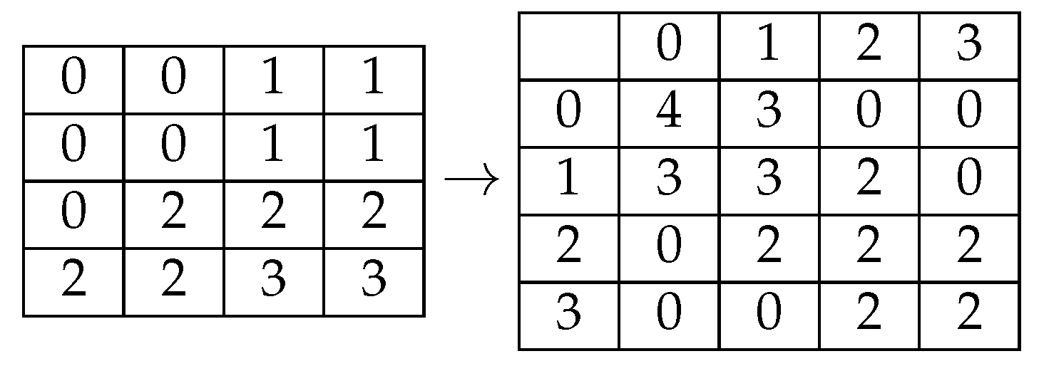
GLCM is a second-order statistical method that estimates the frequency of pixel pairs having the same gray levels in an image and applies additional knowledge gained from spatial relationships. The Co-occurrence matrix incorporates the distribution of grayscale transitions using information from edges. Since most of the information is needed to calculate threshold values in GLCM, it is a simple but effective technique. Consider as an image with 0 to L quantized gray levels, L is taken to be 256. Each element of the GLCM matrix contains the second-order statistics and probability values of the changes between gray levels i and j for a given shift and angle. For a given distance, four angular GLCMs are defined 0 for =
,
,
and
[
20]. Image textures are represented by texture features, which are extracted using texture operators. Gray-level co-occurrence matrices (GLCMs) are one of several texture operators. GLCM is a second-order statistical texture feature used to identify surface texture or microstructure. GLCM is an important tool in terms of ease of calculation and use, as well as its ability to determine surface structure and its ability to determine roughness, roughness, and orientation in a single calculation [
21]. The GLCM is a matrix of the frequency with which multiple sets of pixels exist in gray levels in an image. The GLCM is calculated for a selected pair of distance and angle. For a specific pair of distance and angle the relative recurrences of that pair are calculated for each pixel and its neighbors [
22]. The conclusion is that the GLCM matrix is a statistical method and is easily applicable in images to obtain characteristics related to texture.
2.6. Clustering
2.6.1. Elbow Method
The elbow method involves empirically identifying the best partition of objects by iteratively evaluating the inertia values for different numbers of clusters, aggregating the results, and selecting the optimal result [
23]. In addition to its simplicity by determining the ideal number of clusters that are determined with the sum of the mean square errors or also called inertia.
2.6.2. K-Means
Nowadays, the field of artificial intelligence has provided learning algorithms that have led to the automation of some processes both in industry and in technology. These algorithms are divided into supervised and unsupervised algorithms. The k-means algorithm allows determining the position of k centroids that evenly distribute a set of patterns. It should be noted that, unlike the previous algorithms, this algorithm has the particularity of needing to know a priori the number k of existing classes [
24]. The unsupervised algorithm k-means groups a set of data about its characteristics, forming k groups called clusters.
2.7. Data Augmentation
Data augmentation is one of the effective regularization techniques that aims to prevent overfitting of a network and increase the generalization performance. Data augmentation techniques create richer training data, transformed from the original so that the trained network obtains a higher generalization performance on unseen test data [
25]. Data augmentation is a strategy for increasing the number of records in a dataset when the problem arises of having an adequate level for the machine learning algorithm to learn. Data augmentation can regulate the dataset without increasing the bias. Although the data augmentation technique is well known in imaging, it can also be used in a dataset of numerical variables. The pairing of each cluster is performed by SMOTE, an oversampling technique to level each cluster as shown in
Table 1, identifying the nearest neighbors and generating new data.
Table 1 shows the description and number of clusters.
2.8. Machine Learning
Machine Learning (ML) is a subset of artificial intelligence, in which machines learn to complete a certain task without being explicitly programmed to do so. ML refers to the process of creating a mathematical model on sample data sets called prediction and decision data. ML, a sub-branch of artificial intelligence developed from learning, is a system that investigates the operating principle of algorithms that can make predictions through data [
14]. Depending on the problem posed and the data available, we can distinguish three types of ML: supervised learning, unsupervised learning, and reinforcement learning. While many applications in electronic markets use supervised learning, for example, to predict stock markets [
15]. For the detection of things, objects, and people in addition to automating processes in industries, it also provides many advantages in different areas of study.
2.8.1. SVM
SVM is a powerful method for building a classifier. Its goal is to create a decision boundary between two classes that allows the prediction of labels from one or more feature vectors [
33]. The SVM algorithm is one of the supervised machine learning algorithms based on statistical learning theory. It selects from the training samples a set of character subsets such that the classification of the character subset is equivalent to the division of the entire data set. SVM has been used to successfully solve different classification problems in many applications [
16]. The support vector machine algorithm is a type of learning model that allows us to find the best solution using as a fitting criterion the maximization of the margin, where the margin is understood as the shortest distance between the decision boundary and any of the samples.
2.8.2. Decision Tree
The decision tree method is a tree-like flowchart, where each branch represents the results of attribute tests and the leaf node represents certain classes [
17]. A classification tree is very similar to a regression tree, except that it is a classification used to predict a qualitative response rather than a quantitative one. Recall that in a regression tree, the predicted response for an observation is given by the average response of the training observations belonging to the same terminal node. In contrast, in a classification tree, we predict that each observation belongs to the class of training observations that is most frequent in the region to which it belongs [
31]. The decision tree algorithm is a widely used method for classification and prediction tasks, where it has become a great tool and has had good results in various investigations. The data set obtained is divided between 70 percent training and 30 percent test for the classification of the data. For the application of this algorithm on the obtained data set, it is essential to divide the data set into two parts which are a training part and a testing part and this result is compared with the accuracy of 2 other algorithms.
2.8.3. XGBoosts
XGBoost is a scalable, gradient-based implementation. In crop prediction, XGBoost could be used to improve decision trees by strengthening weak ones. Its syntax usually involves the use of XGBClassifier in the XGBoost library. XGBoost is noted for its predictive accuracy, graceful handling of missing data, and efficient processing of large data sets [
26]. It is suitable for tasks where accuracy is crucial, which makes it valuable for optimizing for farmers. It is suitable for tasks where accuracy is crucial, which makes it valuable for optimizing for farmers [
26]. The XGBoost algorithm is also applied to the obtained data set to obtain a clustered data prediction.
It is highly effective at the task of classification and prediction on large amounts of data, having built-in L2 regularization techniques that help prevent overfitting of the model as well as having capabilities to handle missing values.
3. Materials and Methods
3.1. Methodology
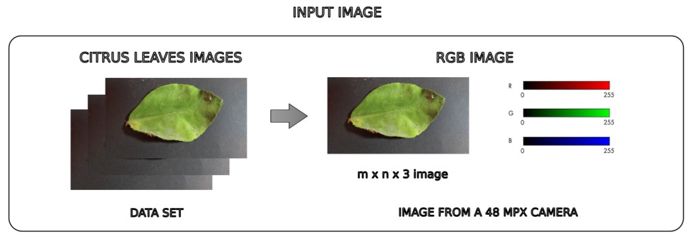
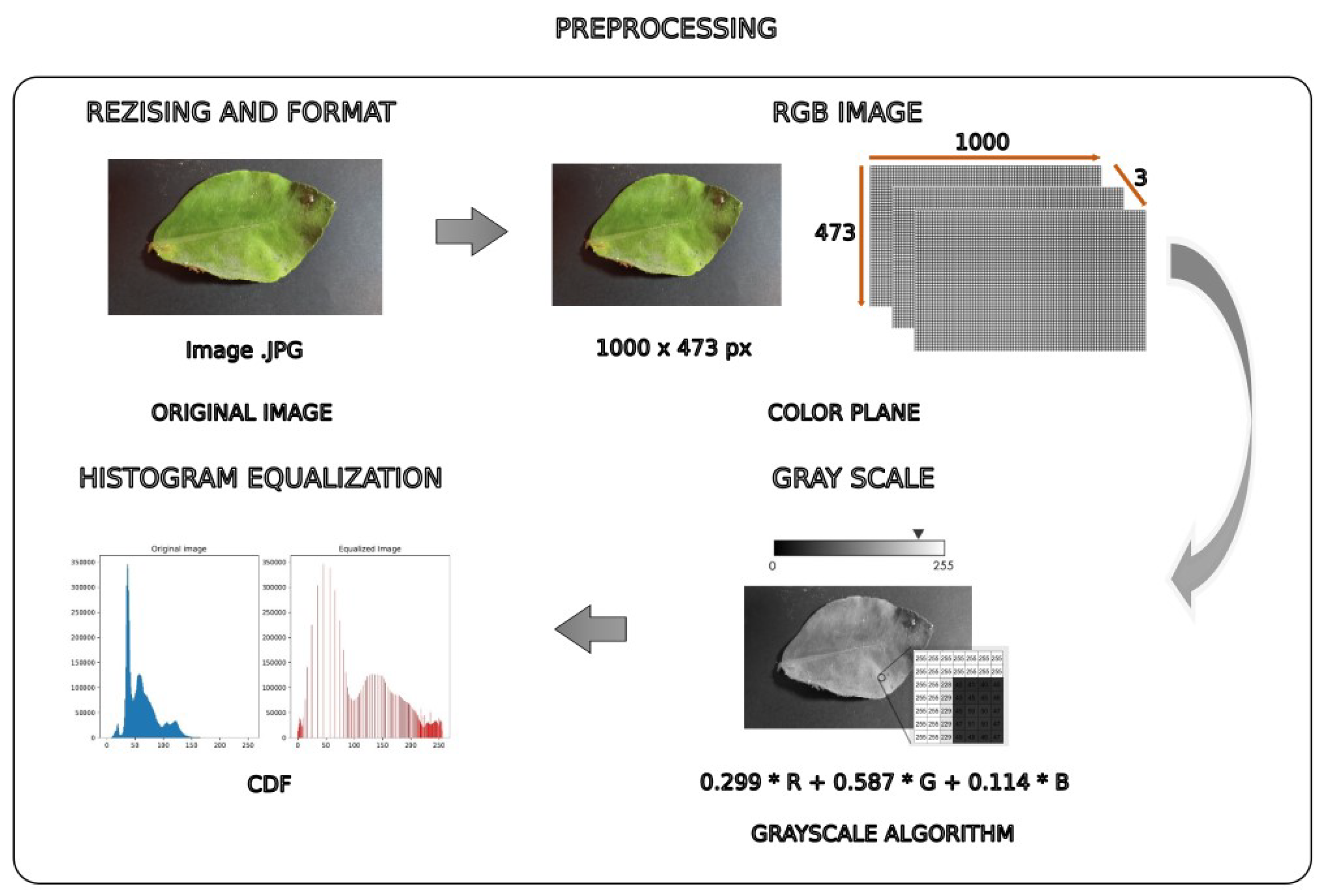
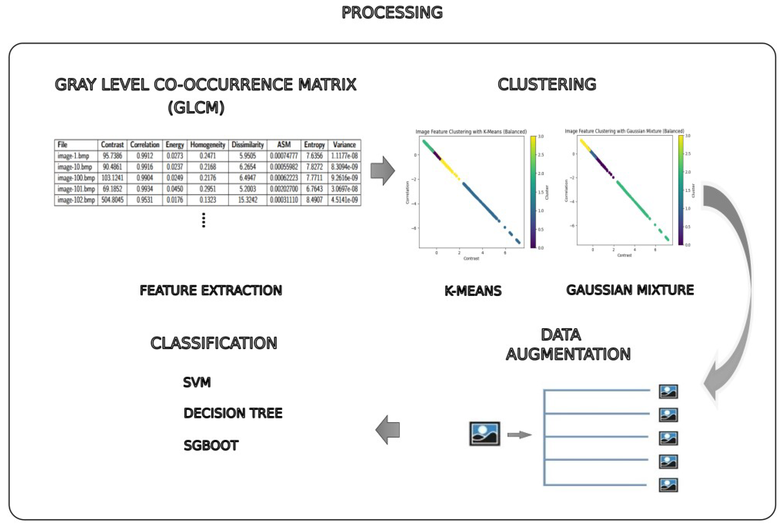
The methodology proposed in the following article is presented in a concise and summarized manner in the following block diagram
Figure 1:
Each of the parts involved in the methodology is a complex system, in which each one consists of a series of steps, which will lead us to achieve the objective of being able to detect the pest leurothrixus floccosus in citrus in
Figure 2,
Figure 3,
Figure 4 and
Figure 5:
3.2. Data Description
The sample obtained are images of leaves of a range of citrus fruits that have been obtained through photographs. In addition, this data has been collected in production centers located in the Valley of Majes, Arequipa, Peru. These photographs present different stages of the plant when the pest infiltrates and develops in the plant having consequences in the growth and production of citrus. In the collection of leaves a random sampling of different trees randomly selected to minimize the bias in the collection of samples is made.
3.3. Image Preprocessing
3.3.1. Image Type and Size
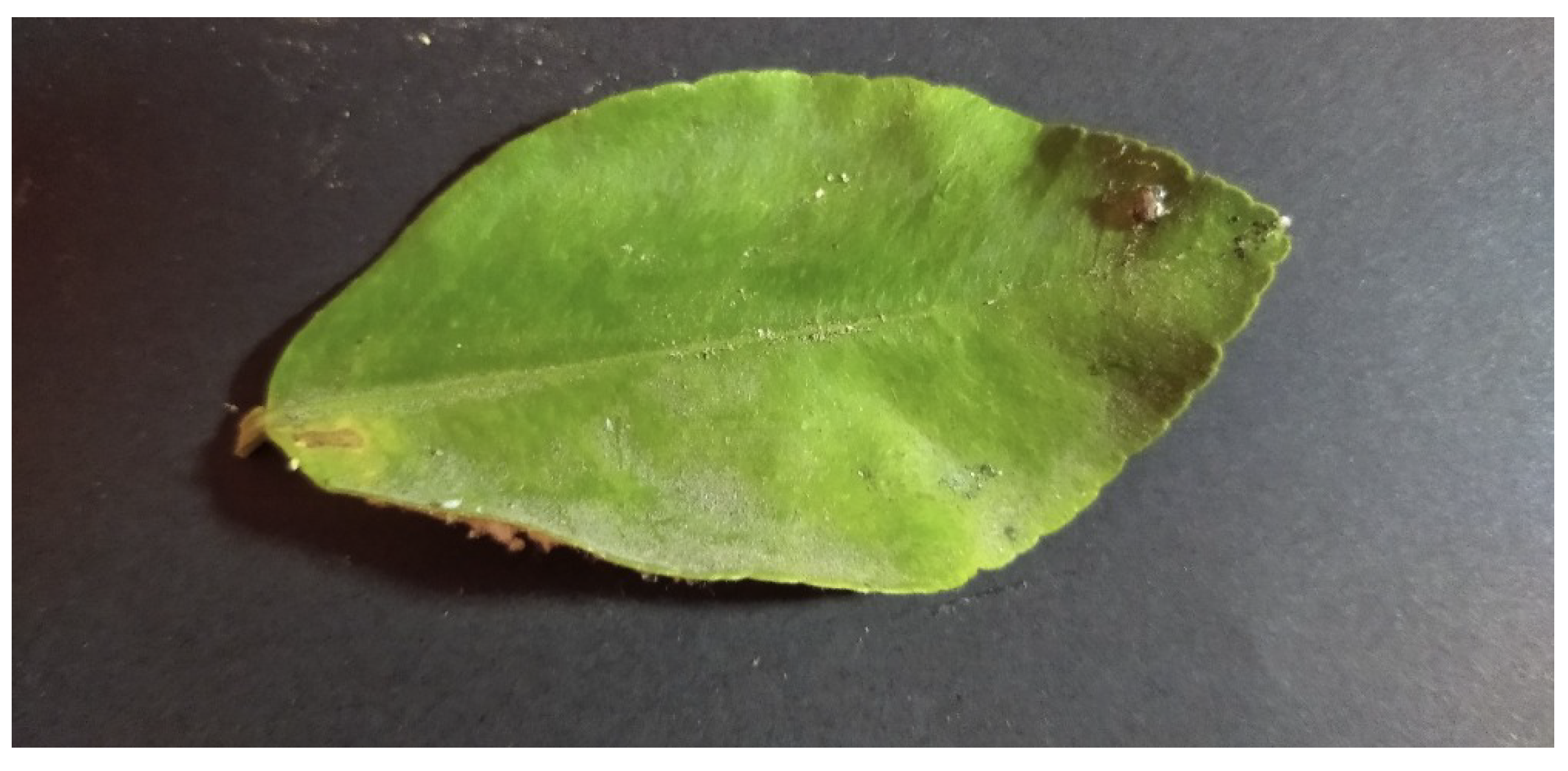
A drone installed with a digital camera was used to take photos of the leaves in the Pedregal region in Arequipa. The type and size of the image are essential for the preprocessing stage. The format used for the images is bmp (bitmap) a format without decompression which allows us to work with a wide variety of information in comparison with other formats such as .jpg which is a compressed format and presents a loss of information in the image, however, this also leads to the image having much less weight, on the other hand, the size of the images is rescaled to
px so that all the data is optimized uniformly in
Figure 6.
3.3.2. Transform
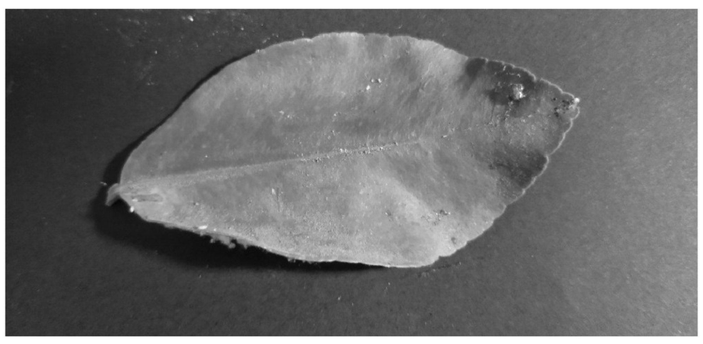
It transforms the rgb image into grayscale due to its easy processing and manipulation, making it easier to work in this format. When converting a color pixel with colors r, g, and b to a grayscale value gv, instead of taking the average of the RGB values, we apply the following conversion formula to calculate gv: [
29].
where:
is the function for color to grayscale conversion and the function round(x) rounds the value of X to an integer representing the grayscale value gv [
30].
Figure 7 is presented the Grayscale.
3.3.3. Histogram Equalization with the Cumulative Distribution Function (CDF)
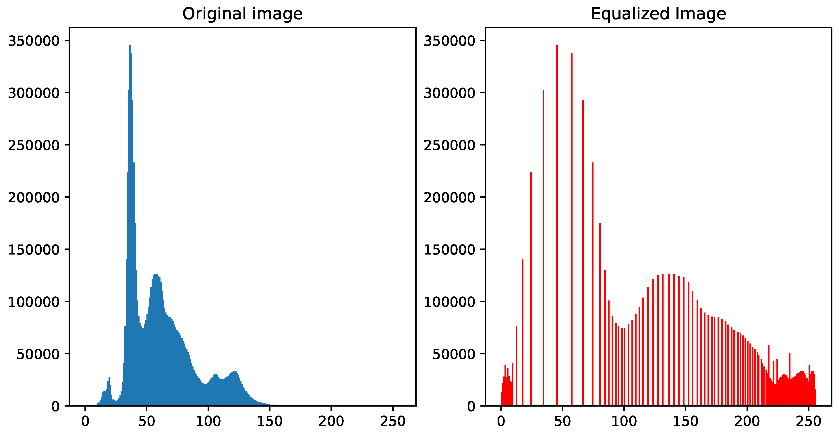
Equalization helps the image so that the distribution of all pixel intensities along the histogram can be distributed equally through equalization as can be seen in
Figure 8. However, it applies in the set of images to adjust the appropriate contrasts for each image. As a result, this leads to the captured images being able to obtain a greater definition of the image object since maintaining the set of pictures without preprocessing them can interfere with the extraction of features and image segmentation. Image equalization process for the distribution of all pixel intensities in the different gray intensities. It is a very common method to adjust the contrast of the image. This is done on all captured images to achieve an equalization of all images. In
Figure 8 is presented the Equalization Histogram.
3.3.4. Noise Reduction
Noise in images a small distortion along the pixel intensity in the image as shown in
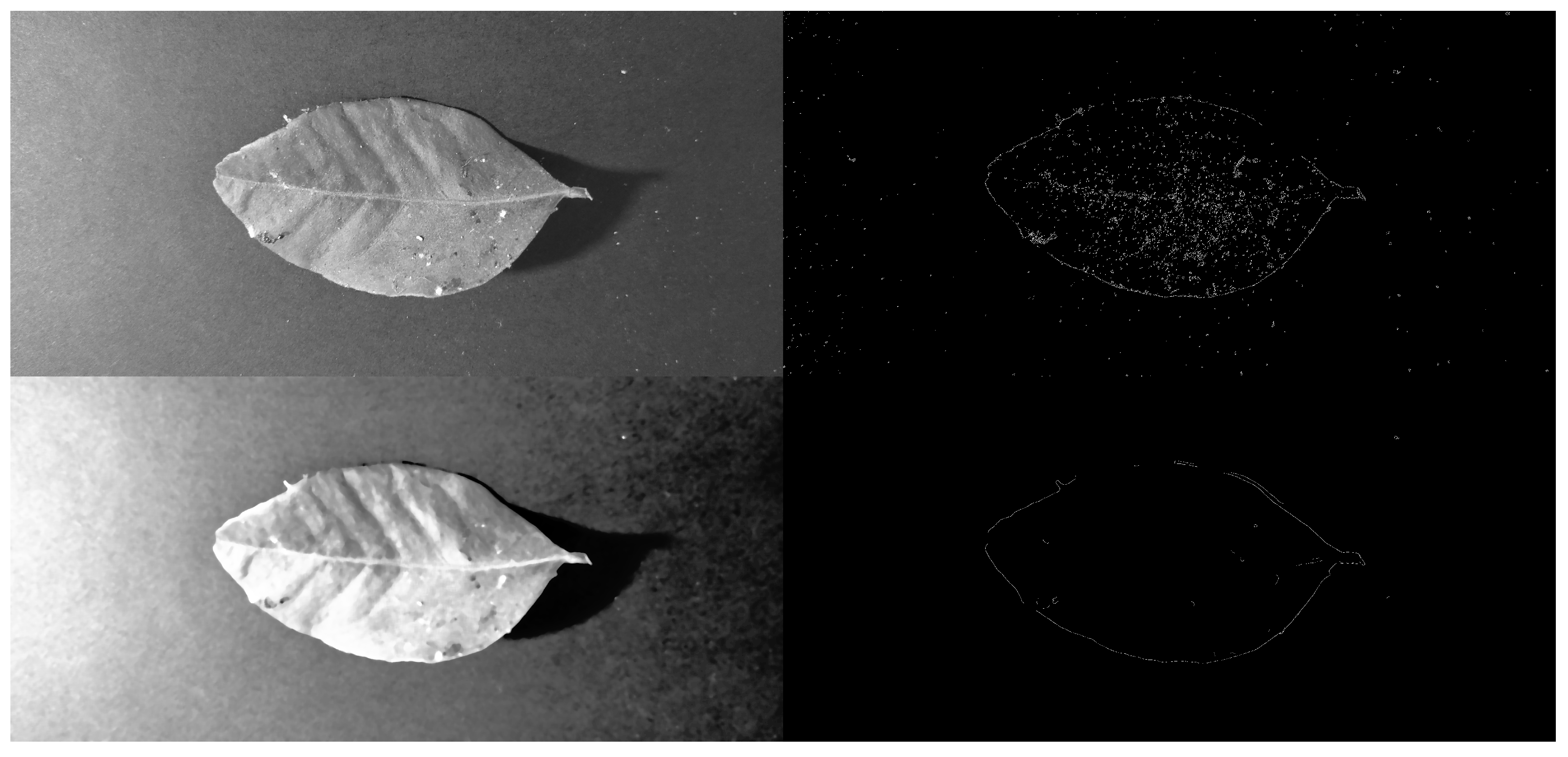
Figure 9, which can modify the result of various techniques that are sensitive to noise in image processing because of this it is essential to eliminate or reduce it. Consequently, in the image, you can identify the salt and pepper class noise that is very common in digital images as well. The median filter is applied on all sets of images for noise reduction with a
kernel that will convolve the entire image eliminating or reducing the white areas in the outer and inner areas of the sheet
Figure 9.
3.4. Image Processing
As seen in
Table 2, each GSLM cell shows how many times the corresponding pair occurs in the original matrix for the defined spatial relationship (d = 1.0°).
3.4.1. Feature Extraction
3.4.1.1. A. Feature description:
Features extracted from the GLCM matrix are as follows:
Constrast: Intensity level of the difference between the gray pixels of the neighboring pixels.
-
where: i, is j, is
Correlation: Correlation level of gray levels in GLCM matrix
Energy: Measurement of image homogeneity
Homogeneity: Measurement of the distance of the elements to the diagonal in the GLCM matrix
Dissimilarity: Difference between the gray levels concerning the neighboring pixels
ASM: Uniformity or regularity of the texture
Entropy:Texture randomness
Variance: Dispersion of the gray levels around the mean
B. Types of variables
In the following
Table 3, we can observe the variables used in the proposed processing.
3.4.2. Determining the Number of Clusters in K-Mean Using the Elbow Method
The elbow method involves empirically identifying the best partition of objects by iteratively evaluating the inertia values for different numbers of clusters, aggregating the results, and selecting the optimal result [
23].
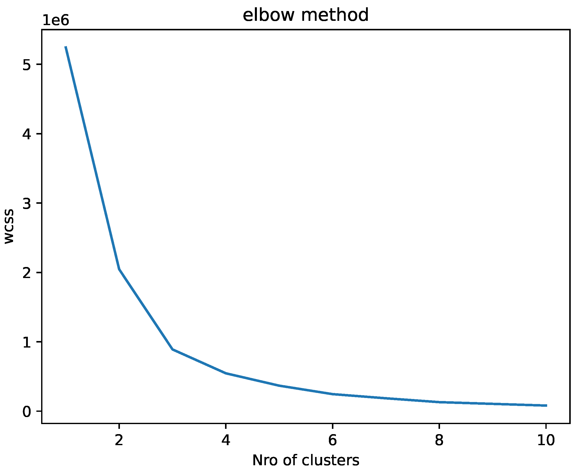
As can be seen in
Figure 10, shows us a graph of a curve, what is sought is to find a point of inflection where the decrease in the sum of least squares within the cluster becomes less pronounced. This point suggests that adding more clusters will not improve data compactness.
Then, using the elbow method we can conclude that the appropriate number of clusters for the analyzed data set is probably 3.
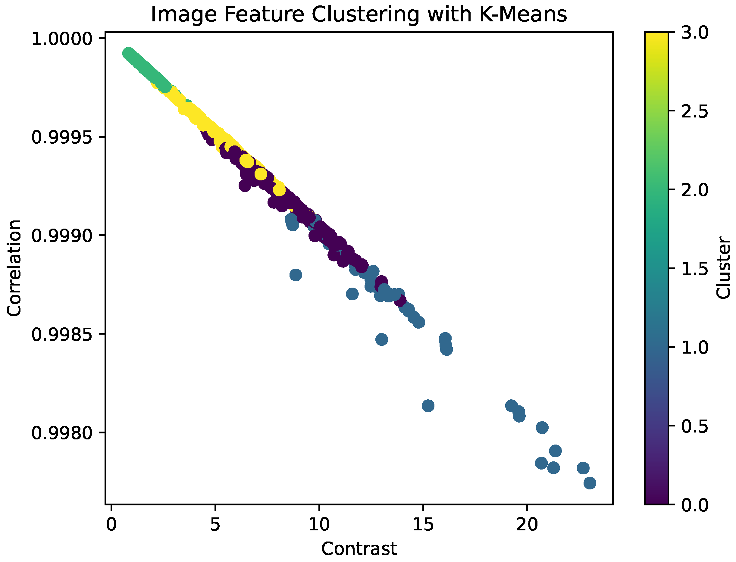
3.4.3. Clustering K-Means
This learning procedure can automatically find the number of clusters without any initialization or parameter selection. We first consider an entropy penalty term to adjust the bias and then create a learning scheme to find the number of groups. In
Figure 11 is shown the clustering K-means.
3.4.4. Clustering Gaussian Mixture
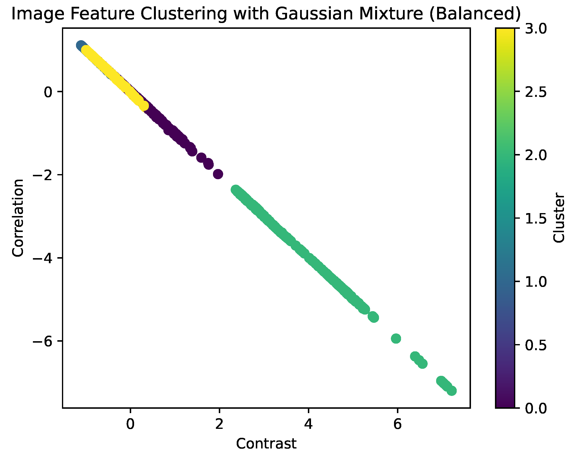
Gaussian mixture models (GMMs) are powerful statistical tools for complex data that do not fit a single distribution. distribution. One of the problems with GMMs is that they require the number of components to be specified in advance [
32]. The segmentation of the data into groups with the same characteristics will be carried out by clustering an unsupervised algorithm. In this process, 4 clustering groups are achieved.
Figure 12 is shown the Clustering. In
Table 4 is shows the Cluster description and number of clusters.
In
Table 5 is shown the quantity of data per cluster.
3.4.5. Segmentation
The segmentation in image processing is mainly one of the most important stages in the study since the detection of the object in the image must be obtained, and at present, there are several segmentation methods. The method employed in the research is edge detection by employing the large derivative of the derivative in the ratio of change from one pixel to another as can be seen in Equations (
11)–(
13) and the second derivative as shown in Equations (
14) and (
15). These equations represent approximations of the second derivative partial of
f with respect to y using finite difference.
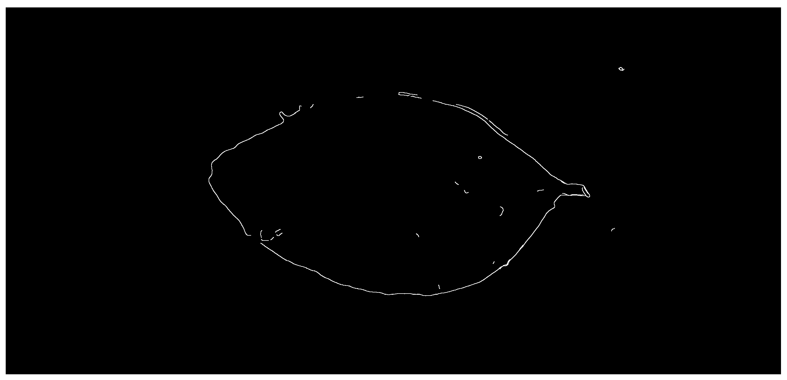
The Canny method works by using grayscale images as input and producing as output or edge images. In its application, the Canny method of edge detection consists of the following steps canny edge detection method, namely smoothing or noise filtering, calculation of gradient magnitude or gradient direction, implementation of non-maximal suppression, set the process of Hysteresis Thresholding. Clustering is a multivariate technique that aims to group similar observations into clusters based on the observed values of several variables for each individual in [
27]. However, the detected edges are not evident in the images because of this problem, and 2 additional methods are presented to strengthen the calculated edges called dilation and closure.
Figure 13 presents the Canny Segmentation.
Bounding Boxes
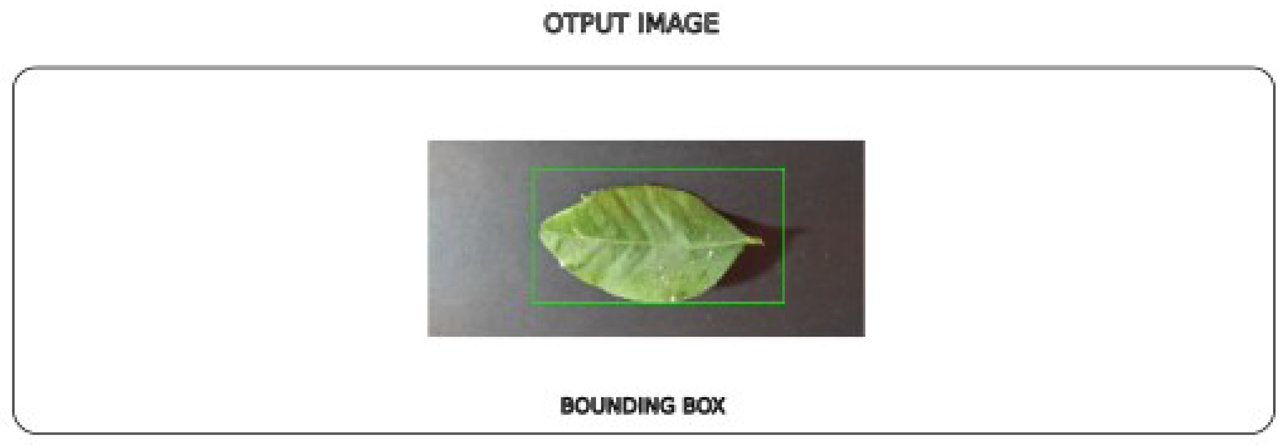
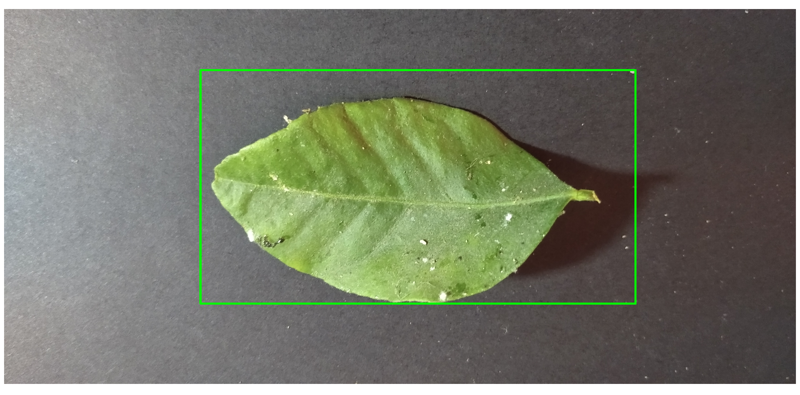
The bounding box is a box that will enclose the target of the image in this case is the leaf with the pest which will be marked in a box as shown in
Figure 14. The capture of the values obtained are the edges of the segmentation when having a sudden change of sharpness in the binary image where it will go through the image row by row looking for a value greater than zero. To finish, the maximum and minimum values of the box are obtained and drawn in the original image.
4. Results and Discussions
In this
Section 4, the results of the methodology proposed in
Section 3 will be presented. To achieve the proposed objectives, three cases will be presented, which are: (a) pre-processing, (b) processing, (c) clustering, (d) classification, and (e) metrics for the evaluation of results.
4.1. Pre-Processing
The data set collected from the leaves of citrus trees was exposed to preprocessing due to the noise they presented, going through the transformation to grayscale for better manipulation, Equalization for the improvement of the image for its intensities, and median filter for the reduction of noise that was presented in the images within the results can be observed in some images the reduction of the noise 87% having remained a little noise salt and pepper in the image and other images can be observed that the 98% of noise eliminating leaving few traces of noise in the image.
4.2. Processing
The processing stage focuses on the operations obtained on the image such as obtaining characteristics that are contrast, correlation, energy, homogeneity, dimilarity, ASM, Entropy, and variance calculated in the glcm matrix. The result is composed of the transformation of images into numerical characteristics converting the image into a vector of characteristics of eight variables.
4.3. Clustering
Clustering is applied in order to group the set of data obtained from the image in groups with the same characteristics due to not having the labeled data set is chosen to perform clustering for identification of the number of clusters is reached to perform the method of the elbow that suggests a range of 2 to 4 clusters so it has opted for 4 clusters in the process as a result we have 4 clusters where you can see the inequality of data for each cluster. Therefore, data augmentation is applied with the method of smote to match the data in each cluster and finally identifies the values of each cluster as shown in
Table 6 and
Table 7.
4.4. Classification
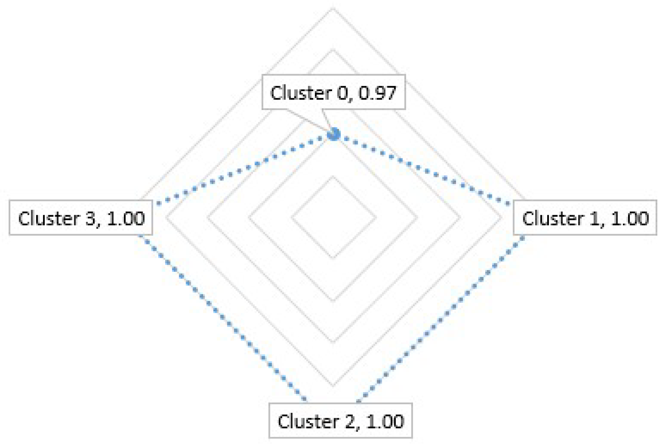
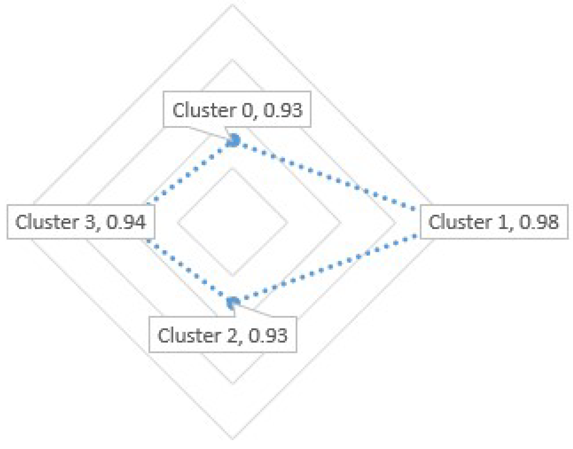
As a result of the proposed methodology for the SVM Model, an accuracy of 97% in the prediction of cluster 0, 100% in the prediction of cluster 1, 100% in the prediction of cluster 2, and 100% in the prediction of cluster 3 is obtained. In
Figure 15,
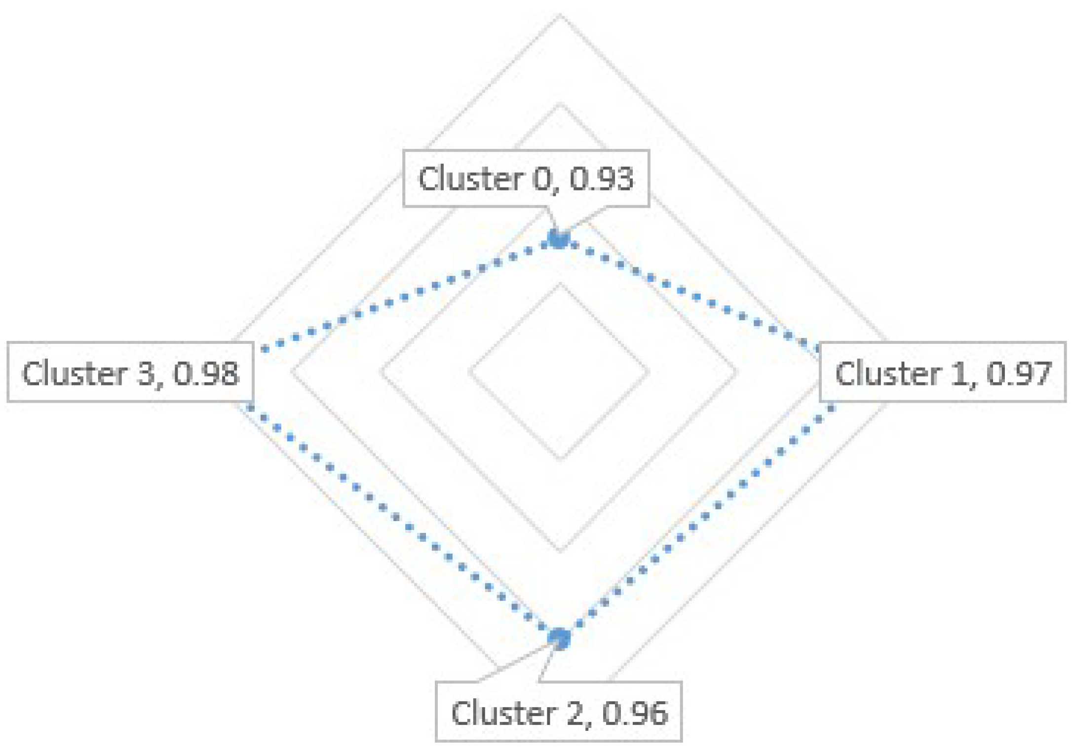
Figure 16 and
Figure 17 compare the accuracies of the SVM Model, XGBoost Model, and Decision Tree Model.
For the XGBoost Model, an accuracy of 93% in the prediction of cluster % in the prediction of cluster % in the prediction of cluster 2, and 98% in the prediction of cluster 3 were obtained.
Finally, for the Decision Tree Model, a precision of 93% in the prediction of cluster % in the prediction of cluster % in the prediction of cluster 2 and 94% in the prediction of cluster 3 was obtained. However, it should be mentioned that other texture methods were not considered to improve accuracy.
If we use the SVM classification method, the highest accuracy will be if we compare the 3 models presented.
4.5. Describe Evaluation Metrics
In
Table 8 is shows the units for Magnetic Properties.
As a result of the proposed methodology, we obtained an accuracy of 89% in the prediction of cluster 0 and 92% in the prediction of cluster 1. Furthermore, we obtained a accuracy of 87% in the prediction of cluster 2, and 100% in the prediction of cluster 3.
5. Conclusions
The aim of this article was to study a proposal for machine learning and image processing techniques in the early detection of diseases in citrus plant leaves using machine learning and image processing techniques such as filters, transformations, and segmentation. Using 1200 captured citrus leaves were used to obtain the results.
In the proposed methodology for the SVM Model, an accuracy of 97% in the prediction of cluster 0, 100% in the prediction of cluster 1, 100% in the prediction of cluster 2, and 100% in the prediction of cluster 3 was obtained. For the XGBoost Model, an accuracy of 93% in the prediction of cluster % in the prediction of cluster % in the prediction of cluster 2, and 98% in the prediction of cluster 3 were obtained. For the Decision Tree Model, a precision of 93% in the prediction of cluster % in the prediction of cluster % in the prediction of cluster 2 and 94% in the prediction of cluster 3 was obtained.
The solution of problems in the detection of patterns in images in some cases can be solved with image processing techniques without entering complex algorithms and robust models as demonstrated in the research, however, the complement of current techniques tends to a better development of research and other areas of knowledge.
The capture of images in different states of the pest greatly influences the results for its detection, being something essential for the understanding of the problem and the proposal of a solution, however, this is not usually a primary determinant of a solution being that also the bad capture of images can be a factor for other questions such as the reconstruction of this one.
Author Contributions
For research articles with several authors, a short paragraph specifying their individual contributions must be provided. The following statements should be used M.A.V.S., J.V.N., G.A.E.E., D.D.Y.A.C. and A.O.S. conceived and designed the study; M.A.V. S., J.V.N., G.A.E.E., D.D.Y.A.C. and J.M.M.V. were responsible for the methodology; M.A.V. S., J.V.N., and J.M.M.V. performed the simulations and experiments; M.A.V.S., J.V.N., J.M.M.V., E.R.L.V. reviewed the manuscript and provided valuable suggestions; M.A.V.S., J.V.N., J.M.M.V. and E.R.L.V. wrote the paper; G.A.E.E., D.D.Y.A.C. and A.O.S. were responsible for supervision. All authors have read and agreed to the published version of the manuscript.
Acknowledgments
This research was funded Universidad Nacional de San Agustin Arequipa (UNSA), through UNSA INVESTIGA (Contract No -UNSA.)
Abbreviations
The following abbreviations are used in this manuscript:
| GMM |
Gaussian mixture models |
| GLCM |
Gray level co-occurrence matrices |
| CDF |
Cumulative Distribution Function |
| SVM |
Support Vector Machine |
| IoT |
Internet of Things |
| WSN |
Wireless sensor networks |
| CNN |
Convolutional Neural Networks |
| DenseNet |
dense convolutional network |
| SMOTE |
Synthetic Minority Over-sampling Technique |
| ANOVA |
Analysis of variance |
| RGB |
Red Green Blue |
References
- Hachimi, C. E.; Belaqziz, S.; Khabba, S.; Sebbar, B.; Dhiba, D.; Chehbouni, A. Smart Weather Data Management Based on Artificial Intelligence and Big Data Analytics for Precision Agriculture. Agriculture (Switzerland) 2023, 13(1), 95. [Google Scholar] [CrossRef]
- Dhaka, V. S.; Meena, S. V.; Rani, G. Sinwar, D. ; Kavita, I. M. F. ; Wozniak, M. A survey of deep convolutional neural networks applied for prediction of plant leaf diseases. Sensors 2021, 21(12), 4749. [Google Scholar] [CrossRef] [PubMed]
- Zhang, Q.; Liu, Y.; Gong, C.; Chen, Y.; Yu, H. Applications of deep learning for dense scenes analysis in agriculture: A review. Sensors 2020, 20(5), 1520. [Google Scholar] [CrossRef] [PubMed]
- Elbasi, E. Mostafa, N. ; Alarnaout, Z. Zreikat, A. I. ; Cina, E. ; Varghese, G. Artificial Intelligence Technology in the Agricultural Sector: A Systematic Literature Review. IEEE Access 2023, 11, 171–202. [Google Scholar] [CrossRef]
- Choudhury, S.; Singh, R.; Gehlot, A.; Kuchhal, P.; Akram, S. V.; Priyadarshi, N.; Khan, B. Agriculture Field Automation and Digitization Using Internet of Things and Machine Learning. Journal of Sensors 2022, 2022(2), 1–17. [Google Scholar] [CrossRef]
- Abdu, A. M.; Mokji, M. M.; Sheikh, U. U. Machine learning for plant disease detection: An investigative comparison between support vector machine and deep learning. IAES International Journal of Artificial Intelligence 2020, 9(4), 670–683. [Google Scholar] [CrossRef]
- Mahmoudi, A.; Benfekih, L. A.; Yigit, A.; Goosen, M. F. A. An assessment of population fluctuations of citrus pest woolly whitefly Aleurothrixus floccosus (Maskell, 1896) (Homoptera, Aleyrodidae) and its parasitoid Cales noacki Howard, 1907 (Hymenoptera, Aphelinidae): A case study from Northwestern Algeria. Acta agriculturae Slovenica 2018, 111(2), 407–417. [Google Scholar] [CrossRef]
- Akhter, R. ; Sofi, S. A. Precision agriculture using IoT data analytics and machine learning. Journal of King Saud University - Computer and Information Sciences 2022, 234(8B), 5602–5618. [CrossRef]
- Luo, D.; Xue, Y.; Deng, X.; Yang, B.; Chen, H.; Mo, Z. Citrus Diseases and Pests Detection Model Based on Self-Attention YOLOV8. IEEE Access, 2023, 11, 139872–139881. [Google Scholar] [CrossRef]
- Li, L. ; Zhang, S. ; Wang. B. Plant Disease Detection and Classification by Deep Learning—A Review. IEEE Access, 2021, 9, 56683–56698.
- Hosny, K. M. El-Hady, W. M. ; Samy, F. M. Vrochidou, E. ; Papakostas, G. A. Multi-Class Classification of Plant Leaf Diseases Using Feature Fusion of Deep Convolutional Neural Network and Local Binary Pattern. IEEE Access, 2023, 11, 62307–62317. [Google Scholar] [CrossRef]
- Shireesha, G. ; Reddy, B. E. Citrus Fruit and Leaf Disease Detection Using DenseNet. 2022 International Conference on Smart Generation Computing, Communication and Networking (SMART GENCON), 2022, 1–5.
- Vélez Serrano, J. F. Vision por Computador. Chapter 3, p. 72. Madrid, España: Paraninfo, 2021.
- Bal, F. ; Kayaalp, F. Review of machine learning and deep learning models in agriculture. International Advanced Researches and Engineering Journal, 2021, 5(2), 309–323. [CrossRef]
- Janiesch, C. ; Zschech, P. ; Heinrich, K. Machine learning and deep learning. Electronic Markets, 2021, 31(3), 685–695. [CrossRef]
- Abdullah, D. M. ; Abdulazeez, A. M. Machine Learning Applications based on SVM Classification: A Review. Qubahan Academic Journal, 2021, 1(2), 81–90. [CrossRef]
- Muchlasin, M. ; Hasbi, M. ; Siswanti, S. Decision Tree Method for Automation of Plant Sprinklers and Monitoring Based On Soil Moisture. Journal Nasional Pendidikan Teknik Informatika (JANAPATI), 2023, 12(1), 25–32.
- Jain, A. K. Fundamentals of Digital Processing. Upper Saddle River, NJ, USA: Prentice-Hall, 1989.
- Kumar, A.; Rout, K. N.; Kumar, S. High Density Salt and Pepper Noise Removal by a Threshold Level Decision based Mean Filter. International Conference on Applied Electromagnetics, Signal Processing and Communication (AESPC), 2018, 1, 1–5. [Google Scholar]
- Xing, Z.; Jia, H. Multilevel Color Image Segmentation Based on GLCM and Improved Salp Swarm Algorithm. IEEE Access, 2019, 7, 37672–37690. [Google Scholar] [CrossRef]
- Prasad, G. ; Gaddale, V. S. ; Kamath, R. C. ; Shekaranaik, V. J. ; Pai, S. P. A Study of Dimensionality Reduction in GLCM Feature-Based Classification of Machined Surface Images. Arab J Sci Eng, 2024, 49(2), 1531–1553. [CrossRef]
- Alazawi, S. A. ; Shati, N. M. ; Abbas, A. F. Texture features extraction based on GLCM for face retrieval system. Periodicals of Engineering and Natural Sciences, 2019, 7(3). [CrossRef]
- Nikiforova, O.; Romanovs, A.; Zabiniako, V.; Kornienko, J. Detecting and Identifying Insider Threats Based on Advanced Clustering Methods. IEEE Access, 2024, 12, 30242–30253. [Google Scholar] [CrossRef]
- Velez Serrano, J. F. Vision por Computador. chapter 5, p. 182. Madrid, España: Paraninfo, 2021.
- Kim, Y.; Uddin, A.F.M.S.; Bae, S. H. Local Augment: Utilizing Local Bias Property of Convolutional Neural Networks for Data Augmentation. IEEE Access, 2021, 9, 15191–15199. [Google Scholar] [CrossRef]
- Ravisha, R. ; Sinha, N. Predictive Model for Smart Agriculture Using Machine Learning. Journal of Mountain Research, 2023, 18(2), 217–222. [CrossRef]
- Riyana Putri, F. N. ; Wibowo, N. C. H. ; Mustofa, H. Clustering of Tuberculosis and Normal Lungs Based on Image Segmentation Results of Chan-Vese and Canny with K-Means. Indonesian Journal of Artificial Intelligence and Data Mining, 2023, 6(1), 18–28. [CrossRef]
- Kalbasi, M.; Nikmehr, H. Noise-Robust, Reconfigurable Canny Edge Detection and its Hardware Realization. IEEE Access, 2020, 8, 39934–39945. [Google Scholar] [CrossRef]
- Hong, W.; Chen, J.; Chang, P. S.; Wu, J.; Chen, T. S.; Lin, J. A Color Image Authentication Scheme With Grayscale Invariance. IEEE Access, 2021, 9, 6522–6535. [Google Scholar] [CrossRef]
- Chen, R. C.; Dewi, C.; Zhuang, Y. C.; Chen, J. K. Contrast Limited Adaptive Histogram Equalization for Recognizing Road Marking at Night Based on Yolo Models. IEEE Access, 2023, 11, 92 926–92 942. [Google Scholar] [CrossRef]
- James, G. ; Witten, D. ; Hastie, T. ; Tibshirani, R. ; Taylor, J. An Introduction to Statistical Learning with Applications in Python. chapter 8, p.337. New York,NY, USA: Springer, 2023.
- Huang, H. ; Liao, Z. ; Wei, X. ; Zhou, Y. Combined Gaussian Mixture Model and Pathfinder Algorithm for Data Clustering. Entropy, 2023, 25(6), 946. [CrossRef]
- Huang, S. ; Nianguang, C. A. I. ; Pacheco, P. P. ; Narandes, S.; Wang, Y. ; Wayne, X. U. Applications of support vector machine (SVM) learning in cancer genomics. Cancer Genomics Proteomics, 2018, 15(1), 41–51. [CrossRef]
|
Disclaimer/Publisher’s Note: The statements, opinions and data contained in all publications are solely those of the individual author(s) and contributor(s) and not of MDPI and/or the editor(s). MDPI and/or the editor(s) disclaim responsibility for any injury to people or property resulting from any ideas, methods, instructions or products referred to in the content. |
© 2024 by the authors. Licensee MDPI, Basel, Switzerland. This article is an open access article distributed under the terms and conditions of the Creative Commons Attribution (CC BY) license (http://creativecommons.org/licenses/by/4.0/).
