Preprint
Article

Random Walk on T-Fractal with Stochastic Resetting

This version is not peer-reviewed.

Submitted:

22 October 2024

Posted:

24 October 2024

You are already at the latest version

A peer-reviewed article of this preprint also exists.

Abstract
In this study, we explore the impact of stochastic resetting on the dynamics of random walks on a T-fractal network. By employing the generating function technique, we establish a recursive relation between the generating function of the first passage time (FPT) and derive a relationship between the mean first passage time (MFPT) with resetting and the generating function of the FPT without resetting. Our analysis covers various scenarios for a random walker reaching a target site from the starting position, and for each case, we determine the optimal resetting probability γ* that minimizes the MFPT. We compare the results with the MFPT without resetting and find that the inclusion of resetting significantly enhances search efficiency, particularly as the size of the network increases. Our findings highlight the potential of stochastic resetting as an effective strategy for optimizing search processes in complex networks, offering valuable insights for applications in various fields where efficient search strategies are crucial.
Keywords: 
Subject: 
Computer Science and Mathematics  -   Probability and Statistics

1. Introduction

Stochastic processes are a fundamental concept in the study of systems that evolve over time in a probabilistic manner. These processes are characterized by randomness and uncertainty, making them ideal for modeling a wide range of phenomena in nature and various scientific disciplines. A particularly important subclass of stochastic processes is the Markov process [1], named after the Russian mathematician Andrey Markov. Markov processes possess the property of memorylessness, meaning that the future state of the system depends only on the present state, not on the sequence of events that preceded it. This property simplifies the analysis of these processes and makes them widely applicable in fields such as statistical physics [2], biology [3,4], finance [5], and computer science [6].
One of the simplest and most extensively studied examples of a Markov process is the random walk. In a random walk, a particle or entity moves step by step in a random direction, with each step being independent of the previous ones. This simple model can represent various real-world scenarios, such as the diffusion of particles in a medium [7], stock price fluctuations [8], and animal foraging behavior [9]. The mathematical tractability of random walks makes them a valuable tool for understanding complex systems and processes.
Applications of random walks span multiple domains. In physics, they are used to model diffusion and transport phenomena, where particles move randomly due to thermal energy [10,11]. In finance, random walks are employed in modeling asset prices and market dynamics, as seen in the famous Efficient Market Hypothesis [12]. In biology, random walks describe the movement patterns of organisms, such as bacteria searching for nutrients [13]. Additionally, random walks are utilized in computer science for algorithms like random search and randomized algorithms, which are used in optimization and data analysis [14].
Stochastic resetting is a fascinating extension of the classical random walk, introducing a mechanism where the walker intermittently returns to a designated position, often referred to as the “resetting point”. This process adds a layer of complexity and control to the otherwise purely random nature of the walk. In a random walk with stochastic resetting, the walker moves according to standard random walk rules but, with a certain probability at each time step, the walker is reset to the initial position. This mechanism can significantly alter the statistical properties of the system, particularly the mean first passage time (MFPT) to a target state.
The concept of stochastic resetting has garnered significant attention due to its counterintuitive ability to optimize certain processes. For example, it has been shown that resetting can minimize the MFPT in search processes, providing a mechanism to escape long periods of inefficient wandering. This has practical implications in various fields, such as optimizing search algorithms [15], enhancing sampling [16], and improving transport phenomena [17]. The idea of resetting has also been linked to various real-world phenomena, such as the process of foraging in animals [9], where a return to a nest or starting point can be advantageous [18].
Theoretical studies of stochastic resetting have explored various aspects, including different resetting protocols (such as resetting to a maximum position instead of the initial one [19]) and the effect of resetting on different types of random walks, such as Lévy flights [20] and anomalous diffusion processes [21]. These studies have demonstrated that the inclusion of a resetting mechanism can lead to a steady-state distribution, even in systems that would otherwise not equilibrate, and can optimize the time to reach a target, under certain conditions [22].
The mathematical framework for analyzing stochastic resetting often involves calculating the MFPT, which measures the expected time for the walker to reach a target state for the first time. The generating function technique is a powerful tool used in these calculations, as it allows for the concise expression of recurrence relations and simplifies the analysis of complex stochastic processes [23]. This approach has been instrumental in deriving exact results for the MFPT and understanding the influence of the resetting rate on the system’s dynamics.
In this paper, we delve into the intricate behavior of random walks on a specific class of fractals known as T -fractals, which belong to the broader family of tree-like fractals. Tree-like fractals are constructed through an iterative process, governed by a positive integer parameter m, and exhibit self-similar patterns at different scales. The T-fractal, in particular, emerges as a special case when m = 1 , exhibiting unique structural properties that make it an ideal candidate for studying random walks and their response to stochastic resetting.
The investigation of random walks on fractals has long been a topic of interest due to their ability to model diffusion processes in complex geometries and heterogeneous media [24,25]. The T-fractal’s hierarchical structure, characterized by its branching nature and increasing complexity with each generation, provides a rich backdrop for exploring how the fractal dimension and other geometrical features affect random walk dynamics.
Our primary focus is on deriving analytical expressions for the Mean first passage time (MFPT) of random walks on the T-fractal, with and without stochastic resetting. Specifically, we consider various scenarios, including walks starting from the outermost nodes, the central node, and randomly selected nodes based on the stationary distribution. For each scenario, we employ generating functions as a powerful tool to tackle the recursive nature of the problem and obtain closed-form solutions for the MFPT.
Furthermore, we extend our analysis to include the effect of stochastic resetting on these random walks. By incorporating resetting events that occur at a fixed rate, we investigate how this mechanism modifies the MFPT and determine the optimal resetting probability that minimizes the MFPT. Such findings offer valuable insights into the design of efficient search strategies and the dynamics of diffusion-limited processes in fractal-like environments.
In summary, this paper contributes to the understanding of random walks on complex networks by providing a comprehensive analysis of random walks and stochastic resetting on the T-fractal. Our results not only deepen the theoretical foundation of this field but also have potential implications for various applications, including target search in complex media, diffusion-controlled reactions, and optimization problems on fractals.
and uncomment

2. Network Model and Some Porperties

2.1. The Construction of the Tree-Like Fractals

Firstly, let’s delve into the overarching network architecture of the T-fractal, which is categorically known as tree-like fractals [26]. These fractals are constructed through an iterative process and possess a fundamental positive integer parameter, m, which plays a pivotal role in their formation. Let F t signify the tree-like fractals at a particular generation t (where t is a non-negative integer).
The methodology employed in their creation commences with a rudimentary starting point involving two nodes that are linked by a solitary edge, which is denoted as F 0 . This foundational configuration serves as the building block for more complex iterations that follow. For t values that are greater than or equal to 1, the fractal F t is pieced together by inserting a new vertex at the midpoint of each existing edge within F t 1 . This innovative vertex is then seamlessly connected to both terminal points of the original initial edge. The process does not end there, as m additional edges are appended to the nodes that were recently introduced into the structure.
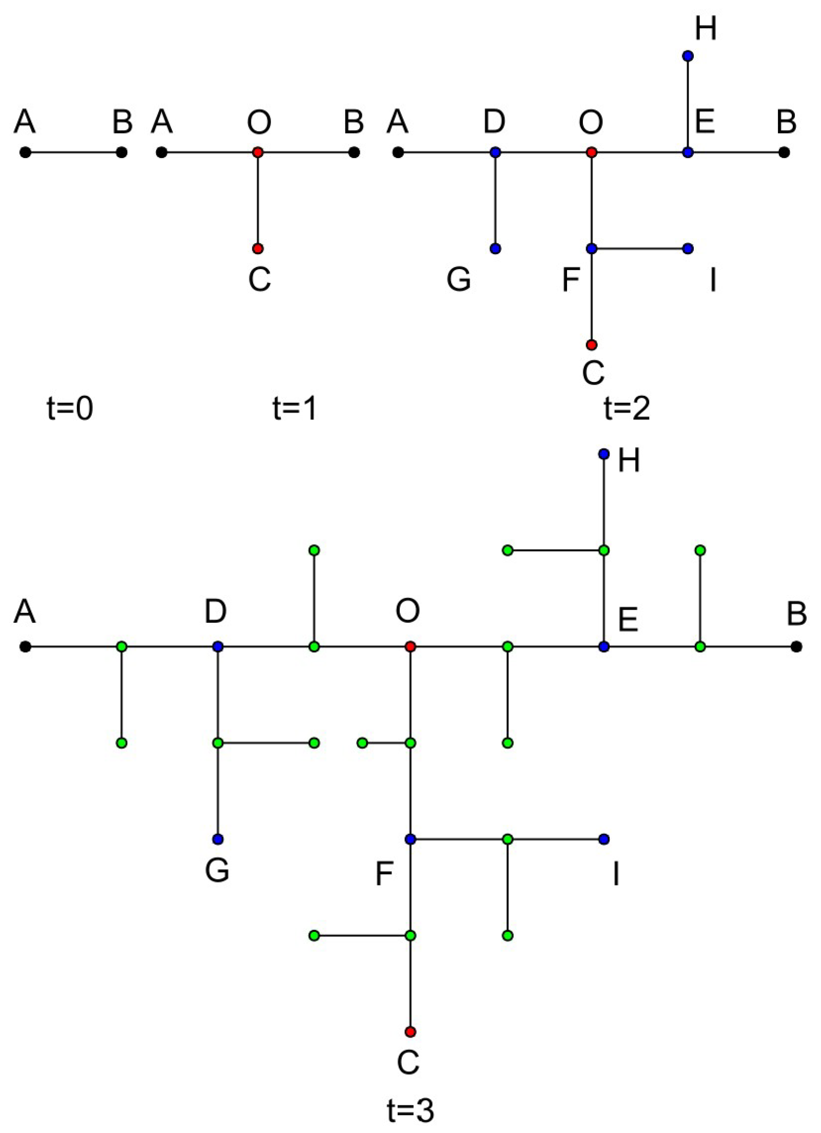
For visual clarity, Figure 1 provides a graphical representation of the initial generation network’s structure when various values of m are chosen. Figure 2 further elucidates the composition of each generation within the tree-like fractals when m is set to 1, a scenario also referred to as the T-fractal. In this figure, the nodes that are generated at disparate generations are depicted using a array of colors, which serves as a helpful tool for comprehending the composite nature of the T-fractal. In this vibrant depiction, the color black is utilized to designate nodes that are born in the zero generation, while the color red is employed to mark the nodes from the first generation. The hue blue is assigned to represent the nodes from the second generation, followed by green for the third generation, and so forth, thereby providing a vivid and clear illustration of the fractal’s generational growth.
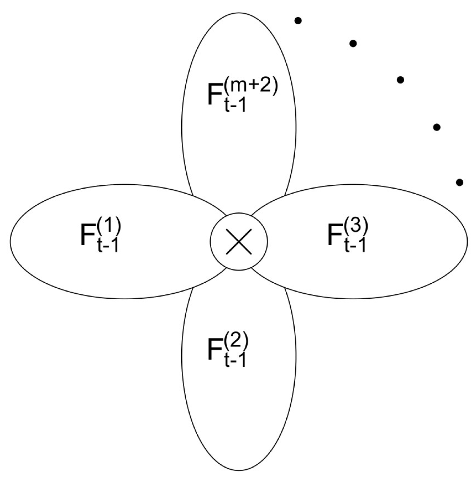
It is worth mentioning that there is another way to construct the tree-like fractals. If we look at it from the first generation, the central node O of the first generation is regarded as the innermost node, and the node farthest from the center is regarded as the outermost node. Then can be regarded as m+2 copies of , connecting the outermost vertex and the innermost vertex, as shown in Figure 3.

2.2. Some Basic Properties of the Tree-Like Fractals

According to the tree-like fractals construction method, the number of edges in each generation of the network is m + 2 times that of the previous generation. Therefore, we can easily conclude that the number of edges in the t-th generation of the tree-like fractals is E t = ( m + 2 ) t . According to the fact that the number of vertices in the tree structure is 1 more than the number of edges, we can conclude that the number of vertices in the t-th generation of the network is N t = ( m + 2 ) t + 1 .
In addition, after each iteration, the diameter of the fractals (i.e., the distance from the innermost node to the outermost node) doubles. Since the number of network edges increases by m + 2 times, we can conclude that the tree dimension is d f = ln ( m + 2 ) ln 2 . In addition, one found that [27] in the spectral for any two nodes i and j in the current generation, the mean first passage time (MFPT) from node i to node j will increase by 2 ( m + 2 ) times in the next generation. Therefore, the dimension of the tree walk is
d r = ln [ 2 ( m + 2 ) ] ln 2 = 1 + d f ,
and the spectral dimension is
d = 2 d f d r = 2 ln ( m + 2 ) ln [ 2 ( m + 2 ) ] = 2 d f 1 + d f .

3. Random Walk on T-Fractal

In this section, we will discuss the random walk on the T-fractal. The structure of T-fractal is shown in Figure 2. It is a special case of tree-like fractal when m = 2 . A similar method can be used to derive the expression of the walk when m takes other values. We will study the MFPT of random walks from the two outermost points (that is, the random walk between A and B), and then based on this, study the random walks in the two outer points (such as the random walk between D and E), and finally derive the random walk starting from the center O. Let’s start with the random walk between A and B.

3.1. Random Walk from A to B

In this subsection, we study the properties of the first passage time (FPT) from A to B (see Figure 2). In order to calculate the generating function of FPT, we set A as the starting point and B as the absorption domain, assuming that the FPT from A to B is a random variable T A B ( t ) , and let P ( t , n ) be the first passage probabilities (FPP). Suppose the generating function of T A B ( t ) is Φ T A B ( t , z ) . Therefore, according to the definition of the generating function (see Appendix A), we can get the probability generating function of T A B ( t ) as:
Φ T A B ( t , z ) = n = 0 + P ( t , n ) z n
Where t represents the generation of the T-fractal.
Now, we denote Ω the set of node in generation 1, which includes nodes A , B , C , O . For any path π starting at node A and reaches B, we use v i denote the node in F t that reaches at time i. In that way, we can denote the way as: π = ( v 0 = A , v 1 , , v T A B ( t ) = B ) . Also, we introduce the observable τ i = τ i ( π ) to represent the time taken to reach for the i-th time any node in Ω along with the path π . The time can be defined as the following way:
τ 0 ( π ) = 0 ,
τ i ( π ) = min { k : k > τ i 1 , v τ i Ω , v τ i v τ i 1 }
And we call N = min { i : v τ i = B } . In fact, N stands for the first passage time in the random walk on the generation 1 (or set Ω ). So if we only consider the random walk in the set Ω , the path π can be simplified as:
σ ( π ) = ( v τ 0 , v τ 1 , , v τ N )
The simplified path σ ( π ) only includes nodes that generated in generation 1, and of course, the interval time between the two steps in σ ( π ) is stochastic. So we can denote the random variable η i the interval time between v τ i 1 and v τ i , as to say,
η i = τ i τ i 1
According to the second T-fractal construction method, F t can be regarded as composed of three F t 1 , and there are two points in A, B, C, O as the endpoints of F t 1 . Therefore, we can infer that η i has the same distribution, and they have the same distribution as T A B ( t 1 ) , and the generating function is Φ T A B ( t 1 , z ) . Moreover, N is the FPT wandering in the first generation, and its generating function is Φ T A B ( 1 , z ) . According to the properties of the generating function (see Appendix A) and Equation (5), we can deduce that the generating function of T A B ( t ) satisfies:
T A B ( t ) = τ N τ 0 = i = 1 N η i
According to the second T-fractal construction method, F t can be regarded as composed of three F t 1 , and there are two points in A, B, C, O as the endpoints of F t 1 . Therefore, we can infer that η i has the same distribution, and they have the same distribution as T A B ( t 1 ) , and the generating function is Φ T A B ( t 1 , z ) . Moreover, N is the FPT wandering in the first generation, and its generating function is Φ T A B ( 1 , z ) . According to the properties of the generating function (see Appendix A) and Equation (5), we can deduce that the generating function of T A B ( t ) satisfies:
Φ T A B ( t , z ) = Φ T A B ( 1 , Φ T A B ( t 1 , z ) )
As for the initial condition Φ T A B ( 1 , z ) , it can be derived by transition probability matrix for random walks on T-fractal in generation 1, see exactly in Appendix B, the result is:
Φ T A B ( 1 , z ) = z 2 3 2 z 2
By solving the Equation (6) with initial condition Equation (7), we get:
Φ T A B ( t , z ) = z 2 t 27 36 z 2 3 2 z 2 2 t 1 × ( 3 2 z 2 ) 2 27 36 z 2
Now we turn to calculate the mean first passage time (MFPT) of the random walk Starting from node A and absorbing at node B, we denote it as E ( T A B ( t ) ) , which is the mathematical expectation for the random variable T A B ( t ) . We can derive it through taking derivatives on both sides of the Equation (6), and posing z = 1 (see exactly in Appendix C), we get:
E ( T A B ( t ) ) = 6 t

3.2. Random Walk from D to E

We now use the similar method to calculate the mean first passage time from node D to E. We suppose the random variable T D E ( t ) denotes the first passage time from node D to E in generation t ( t 2 ), where the starting point is D, and the absorbing domain is E. Let Ω 2 denotes the node in generation 2. Like the method to calculate MFPT from A to B, we can only consider the random walk in generation 2, and we use v i to denote the interval time between the random walk in Ω 2 . So the T D E ( t ) can also be written as:
T D E ( t ) = i = 1 N v i
We suppose the generating function of the random variable T D E ( t ) is Φ T D E ( t , z ) . So in this situation, the generating function of random variable N is Φ T D E ( 2 , z ) , since N stands for the random walk from node D to E in generation 2. Now, we analyze the generating function of the random variable v i . It is obvious that v i ( i = 1 , 2 , ) has the identical distribution. For each random walk in generation t, the interval time between the nodes in generation 2 can be seen as the random walk from A to B in generation t 2 . Because no matter what two nodes in generation 2 are, they have as only as two nodes on the edge of the random walk. So we can conclude that the generating function of v i ( i = 1 , 2 , ) are Φ T A B ( t 2 , z ) . So by using the Equation (10) and the properties of generating function (See Appendix A, Equation (A7)), we can conclude that:
Φ T D E ( t , z ) = Φ T D E ( 2 , Φ T A B ( t 2 , z ) )
As for the initial condition Φ T D E ( 2 , z ) , it can also be calculated by using the generating function of the matrix, also see in Appendix B. The result is:
Φ T D E ( 2 , z ) = z 2 6 5 z 2
Similar to the above method, we take derivation to both sides of the Equation (11), see exactly in Appendix C, we can get the MFPT of the random walk from D to E:
E ( T D E ( t ) ) = 2 · 6 t 1

3.3. Random Walk from O to B

Similar to the analysis from the above two situations, we can also use the generating function to calculate the MFPT from node O to B, where O as the innermost node is the starting point of the random walk and B is the absorbing domain. We suppose the random variable T O B ( t ) denote the FPT from O to B in generation t. And the generating function of T O B ( t ) denote as Φ T O B ( t , z ) , similar to the above method, we have:
T O B ( t ) = i = 1 N η i
Where η i is the interval time between random walks in generation 1. The generating function of random variable N is Φ T O B ( 1 , z ) , and the generating function of η i is Φ T A B ( t 1 , z ) . So we can get the following recursion:
Φ T O B ( t , z ) = Φ T O B ( 1 , Φ T A B ( t 1 , z ) )
The initial condition is (see exactly in Appendix B):
Φ T O B ( 1 , z ) = z 3 2 z 2
By taking derivation to both sides of Equation (15), we get (see in Appendix C):
E ( T O B ( t ) ) = 5 · 6 t 1

3.4. Random Walk from O to E

As a comparison of the random walk from O to B, we now discuss the random walk, starting at node O, and absorbing at node E (see in Figure 2). We denote T O E ( t ) as the FPT from O to E in generation t. And the generating function of it denotes as Φ T O E ( t , z ) . With the same method as the random walk from O to B, we get the recursion:
Φ T O E ( t , z ) = Φ T O E ( 2 , Φ T A B ( t 2 , z ) )
With the initial condition:
Φ T O E ( 2 , z ) = z ( 3 2 z 2 ) 6 5 z 2
By taking derivation to both sides of Equation (18), we also get:
E ( T O E ( t ) ) = 7 · 6 t 2

3.5. Random Walk to B with the Starting Node Selected Randomly

In this section, we will discuss a new problem, about the random walk from any point to a given absorbing point. The starting point is selected based on the stationary distribution. Here we first introduce the stationary distribution.
In the context of a random walk, the stationary distribution (also known as the invariant distribution or equilibrium distribution) refers to a probability distribution over the states of the system that remains unchanged as time progresses, assuming the process reaches equilibrium.
For a random walk on a finite state space (such as a Markov chain), the stationary distribution Π satisfies the following condition:
Π = Π P
Here, P is the transition matrix of the Markov chain, where each entry P i j represents the probability of transitioning from i to j.
In the random walk on network, we have the conclusion that:
Π = d 1 k = 1 N d k , d 2 k = 1 N d k , , d N k = 1 N d k
Where d k stands for the degree of the vertex k.
Then, we discuss the random walk to B with the starting site randomly selected according to the stationary distribution Π in Equation (22). We denote the first passage time (FPT) of this random walk in T-fractal as T Π B ( t ) in generation t. And the Φ T Π B ( t , z ) denotes the generating function of T Π B ( t ) . And we also introduce a new concept in random walk, the return time (RT). It is the time that the walker returns to the initial node. We denote the return time to B as T B B ( t ) in generation t of the T-fractal. And the generating function of the T B B ( t ) is Φ T B B ( t , z ) . It has been found that there is a relationship between Φ T Π B ( t , z ) and Φ T B B ( t , z ) (See [30] exactly):
Φ T Π B ( t , z ) = z 1 z × d B 2 E × 1 Φ T B B ( t , z )
Where d B stands for the degree of node B, and E is the total number of edges of the network. Replacing d B = 1 and E ( t ) = 3 t into Equation (23), we get:
Φ T Π B ( t , z ) = z 1 z × 1 2 × 3 t × 1 Φ T B B ( t , z )
About the Φ T B B ( t , z ) , we have the following equations (See Appendix ):
Φ T B B ( t , z ) = Φ T B B ( t 1 , z ) Ψ ( Φ T A B ( t , z ) )
with:
Ψ ( z ) = Φ T B B ( 0 , z ) Φ T B B ( 1 , z )
With the initial condition Φ T B B ( 0 , z ) = 1 1 z 2 and Φ T B B ( 1 , z ) = 3 2 z 2 3 ( 1 z 2 ) (see in Appendix B), we get:
Ψ ( z ) = 3 3 2 z 2
Combine with Equation (24) (25) (27), we get:
Φ T Π B ( t , z ) = 2 Ψ ( Φ T A B ( t 1 , z ) ) × Φ T Π B ( t 1 , z )
With the initial condition:
Φ T Π B ( 0 , z ) = 1 2 z ( z + 1 )
By calculating the derivatives to both sides of the Equation (29) and posing z = 1 , we get the MFPT of this random walk:
E ( T Π B ( t ) ) = 4 5 · 6 t + 7 10 4 5 · 6 t

4. Random Walk on Network with Stochastic Resetting

In this section, we provide a general method for calculating the MFPT in a general network with stochastic resetting. Then, we study the MFPT in general discrete-time random walk with a fixed resetting rate in general network. The findings in this section will help us to determine the random walk with stochastic resetting in a specific network, such as the T-fractal which we discuss in this article.

4.1. MFPT for the Discrete-Time First Passage Process under Resetting

Random walk with stochastic resetting are characterized by restarts occurring at a random time. We suppose the resetting was happened on random time R. Let T R refers to the first passage time under resetting, and T refers to first passage time without resetting. One obtain [28,29]:
T R = T T < R R + T R T R
Then, in this section, we will focus on the discrete-time random walk on network with resetting. We will investigate the relationship between the mean of T R and the generating function of T and R. Then, we will calculate the mean of T R by using the generating function. The method was presented by Ref. [29]. Let
I ( T R ) = 0 T < R 1 T R
So we can rewrite Equation (18) as:
T R = min ( T , R ) + I ( T R ) × T R
Let E ( ξ ) denote the first moment (i.e., the mathematical expectation) of the random variable ξ and Pr ( A ) denote the probability the event A occurs. So we obtain:
E ( T R ) = E ( min ( T , R ) ) + E ( I ( T R ) · T R ) = E ( min ( T , R ) ) + Pr ( T R ) · E ( T R ) = E ( min ( T , R ) ) + [ 1 Pr ( T < R ) ] · E ( T R )
Note that the random variable T R and T R are independent and identically distributed. Of course, their first moments are equivalent. So, we can get:
E ( T R ) = E ( min ( T , R ) ) Pr ( T < R )
By the definition of the first moment and some properties, we can get:
E ( min ( T , R ) ) = m = 0 Pr ( min ( T , R ) > m ) = m = 0 k = m + 1 Pr ( T = k ) l = m + 1 Pr ( R = l )
Pr ( T < R ) = m = 0 Pr ( T = m ) l = m + 1 Pr ( R = l )

4.2. MFPT for Random Walk on Network with a Fixed Resetting Rate

Now we discuss the discrete random walk on network with stochastic resetting at a fixed rate. At each step, there is a fixed probability γ to reset to the initial site, we call γ the resetting rate. While, there are probability 1 γ for the walker to walk to the adjacent nodes that the walker currently occupied. So, the random variable R discuss above, which is the time that takes walker to restart to the initial site, follows the geometric distribution with the parameter γ , that is to say, for any l 1 :
Pr ( R = l ) = ( 1 γ ) l 1 γ
This can be explained as, if the walker resets at time l, which means that he doesn’t reset in the ( l 1 ) times before, with the probability ( 1 γ ) l 1 . And he reset at time l, with the probability γ . Therefore, for any m 0 ,
l = m + 1 Pr ( R = l ) = l = m + 1 ( 1 γ ) l 1 γ = ( 1 γ ) m
Substituting Equation (26) in Equation (23) (24), we get:
E ( min ( T , R ) ) = m = 0 [ ( 1 γ ) m k = m + 1 Pr ( T = k ) ] = k = 1 [ Pr ( T = k ) m = 0 k 1 ( 1 γ ) m ] = k = 1 [ Pr ( T = k ) 1 ( 1 γ ) k γ ] = 1 γ [ 1 k = 0 [ Pr ( T = k ) ( 1 γ ) k ] ] = 1 Φ T ( 1 γ ) γ
Also, we get:
Pr ( T < R ) = m = 0 [ Pr ( T = m ) ( 1 γ ) m ] = Φ T ( 1 γ )
Where Φ T ( z ) is the generating function of the random variable T, can be written as:
Φ T ( z ) = k = 0 [ Pr ( T = k ) z k ]
Inserting the Equation (27) (28) into Equation (22), we get an important conclusion:
E ( T R ) = 1 Φ T ( 1 γ ) γ Φ T ( 1 γ )
This formula can be used to calculate mean first passage time (MFPT) with stochastic resetting. Through this formula, we can transform the problem of solving MFPT with resetting into the problem of solving generating function without resetting. It should be pointed out, for any random variable R, if R follows the geometric distribution with parameter γ , the result shown above are also true.
In section II, we have found some recursions about the generating function of the random walk on T-fractal without resetting. And in this section, we have found a relationship between the MFPT of the random walk with stochastic resetting at a fixed resetting rate and the generating function without resetting. So in the next section, we will combine the two findings above and conclude the MFPT of the random walk on T-fractal with stochastic resetting.

5. Random Walk on T-Fractal with Stochastic Resetting

In this section, we discuss the MFPT for different random walk on the T-fractal. We determine different resetting site. And the resetting site is the starting site. For each random walk, we will discuss the optimal γ to make the MFPT minimum. The results presented in this section will provide the resetting strategy to enhance the search efficiency, as measured as MFPT. So let’s start with random walk from O to B with resetting.

5.1. Random Walk with Resetting from O to B

We now discuss the random walk on T-fractal with resetting from O to B. The walker starts the random walk from node O, and the absorbing node is B. At each step, there is a probability γ for the worker to reset to the initial site O, and there is probability 1 γ for the walker to walk through the adjacent node. By solving the Equation (15) with the initial condition (16), we can get the generating function for the first passage time from node O to B without resetting. The result is:
Φ T O B ( t , z ) = ( 2 2 t 1 + t 4 ) z ( 3 2 t 1 × 2 2 t 1 + t 3 + 2 2 t + 2 t 7 ) z 2 + 3 2 t 1
Therefore,
Φ T O B ( t , 1 γ ) = 2 2 t 1 + t 4 2 2 t 1 + t 4 γ ( 3 2 t 1 × 2 2 t 1 + t 3 + 2 2 t + 2 t 7 ) γ 2 2 ( 3 2 t 1 × 2 2 t 1 + t 3 + 2 2 t + 2 t 7 ) γ
Let E ( T O B R ( t ) ) denote the first moment of the random walk from O to B with resetting in generation t. So, by the Equation (30), we have:
E ( T O B R ( t ) ) = 1 Φ T O B ( t , 1 γ ) γ ϕ T O B ( t , 1 γ ) = ( 3 2 t 1 × 2 2 t 1 + t 3 + 2 2 t + 2 t 7 ) γ 2 [ 2 ( 3 2 t 1 × 2 2 t 1 + t 3 + 2 2 t + 2 t 7 ) + 2 2 t 1 + t 4 ] γ 2 2 t 1 + t 4 2 2 t 1 + t 4 γ + 3 2 t 1 2 2 t 1 + t 4 2 2 t 1 + t 4 2 2 t 1 + t 4 γ
By taking the first-order derivative with respect to γ on both sides of Equation (46), and setting γ E ( T O B R ( t ) ) = 0 , we get:
[ ( 3 2 t 1 × 2 2 t 1 + t 3 + 2 2 t + 2 t 7 ) 2 2 t 1 + t 4 + 2 2 t + 2 t 8 ] γ 2 + [ 2 2 t + 2 t 7 2 ( 3 2 t 1 × 2 2 t 1 + t 3 + 3 2 t 1 ) 2 2 t 1 + t 4 ] γ + [ ( 3 2 t 1 × 2 2 t 1 + t 3 + 2 2 t + 2 t 7 ) 2 2 t 1 + t 4 2 2 t + 2 t 8 ] = 0
So we can get the root (the negative root was removed):
γ O B * = 1 2 2 t + 2 t 7 + 2 3 2 t 1 × 2 2 t 1 + t 3 + 2 2 t + 2 t 7 + 3 2 t 1 2 2 2 t 5 2 ( 3 2 t 1 × 2 2 2 t 4 + 2 2 t + 2 t 7 ) 2 2 t 1 + t 4 + 2 2 t + 2 t 8 2 2 t + 2 t 7 2 3 2 t 1 × 2 2 2 t 5 + 2 2 t + 2 t 7 + 3 2 t 1 2 2 2 t 5 2 ( 3 2 t 1 × 2 2 2 t 4 + 2 2 t + 2 t 7 ) 2 2 t 1 + t 4 + 2 2 t + 2 t 8
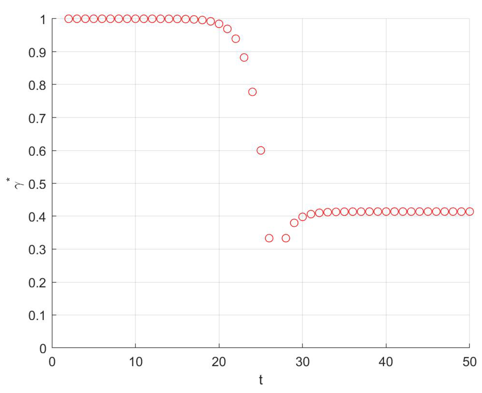
By plotting the γ O B * as a function of t (see Figure 4), we find for at any generation t, the optimal solution of the Equation (47) γ * ( 0 , 1 ) . We also find that from t = 20 , the γ * decreases, and from t = 27 , γ * increase again. And the minimum of the γ * is 0.33 when t=27. And when t , γ * 2 1 0 . 41 .
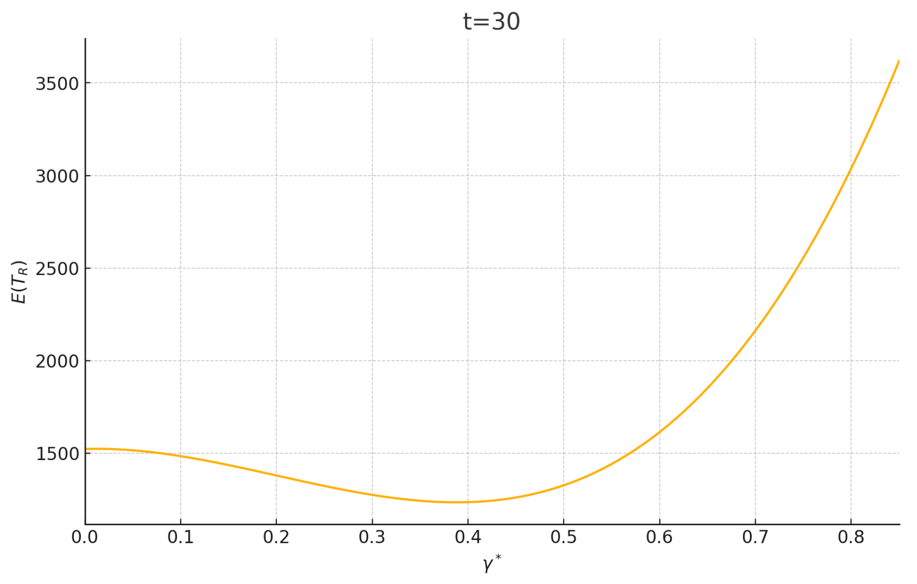
And Figure 5 shows that when t = 30 , the MFPT of the random walk from O to B with the resetting rate γ . We find the optimal γ is about 0.40 where the MFPT becomes the smallest. By performing numerical calculations, we find the ratio of MFPT in random walks with and without resetting when t :
lim t E ( T O B ( t , γ ) ) γ = γ * E ( T O B ( t ) ) 2 3
This shows that when the network size is very large, resetting can improve the efficiency of random search from the central O to the outer most side .

5.2. Random Walk with Resetting from O to E

We now discuss the random walk with resetting from O to E. At each step, there is probability γ for the walker to reset to the initial position O. And there is probability 1 γ for the walker to walk to the adjacent node from the current position. By solving the Equation (18) with the initial condition (19), we get the generating function of T O E ( t ) without resetting:
Φ T O E ( t , z ) = ( 9 × 2 t 4 2 t 1 × 3 2 t 2 5 t + 6 ) z 2 4 t 1 ( 2 2 t 3 × 3 2 t 2 6 t + 8 ) z + 4 t × 27 ( t 2 ) 2 z 2
Therefore,
Φ T O E ( t , 1 γ ) = ( 9 × 2 t 4 2 t 1 × 3 2 t 2 5 t + 6 ) ( 1 γ ) 2 4 t 1 ( 2 2 t 3 × 3 2 t 2 6 t + 8 ) ( 1 γ ) + 4 t × 27 ( t 2 ) 2 ( 1 γ ) 2
So, the MFPT with resetting can be calculated as:
E ( T O E R ( t ) ) = 1 Φ T O E ( t , 1 γ ) γ Φ T O E ( t , 1 γ ) = 4 t 1 ( 2 2 t 3 × 3 2 t 2 6 t + 8 ) ( 1 γ ) + 4 t × 27 ( t 2 ) 2 ( 1 γ ) 2 γ ( 9 × 2 t 4 2 t 1 × 3 2 t 2 5 t + 6 ) ( 1 γ ) 2 ( 9 × 2 t 4 2 t 1 × 3 2 t 2 5 t + 6 ) ( 1 γ ) 2 γ ( 9 × 2 t 4 2 t 1 × 3 2 t 2 5 t + 6 ) ( 1 γ ) 2
By taking the derivative to Equation (51), and letting d d γ E ( T O E R ( t ) ) = 0 , we get:
[ 4 t × 27 ( t 2 ) 2 ( 9 × 2 t 4 2 t 1 × 3 2 t 2 5 t + 6 ) ] γ 2 + [ 2 2 t 3 × 3 t 2 6 t + 8 2 × 4 t × 27 ( t 2 ) 2 + ( 9 × 2 t 3 2 t 1 × 3 2 t 2 5 t + 6 ) ] γ + 4 t 1 + 9 × 2 t 4 2 t 1 × 3 2 t 2 5 t + 6 = 0
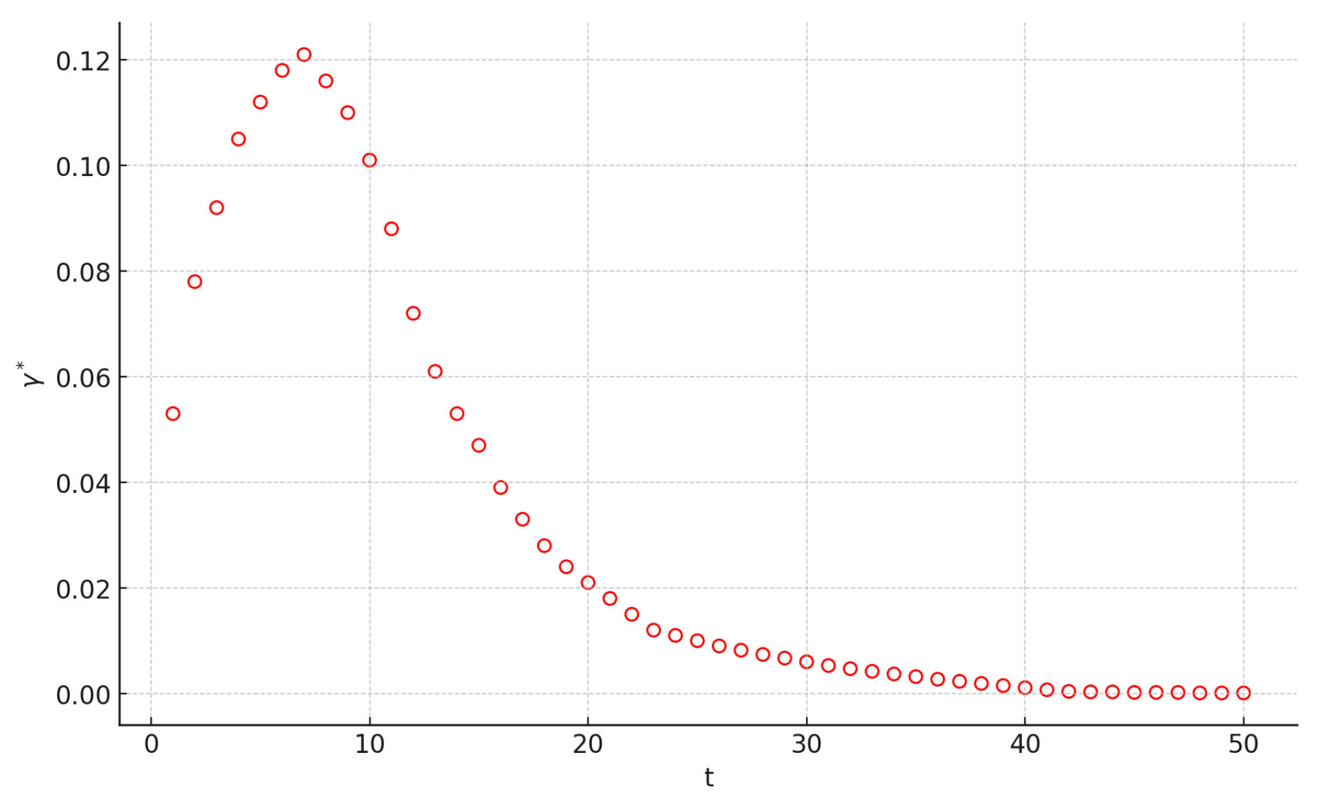
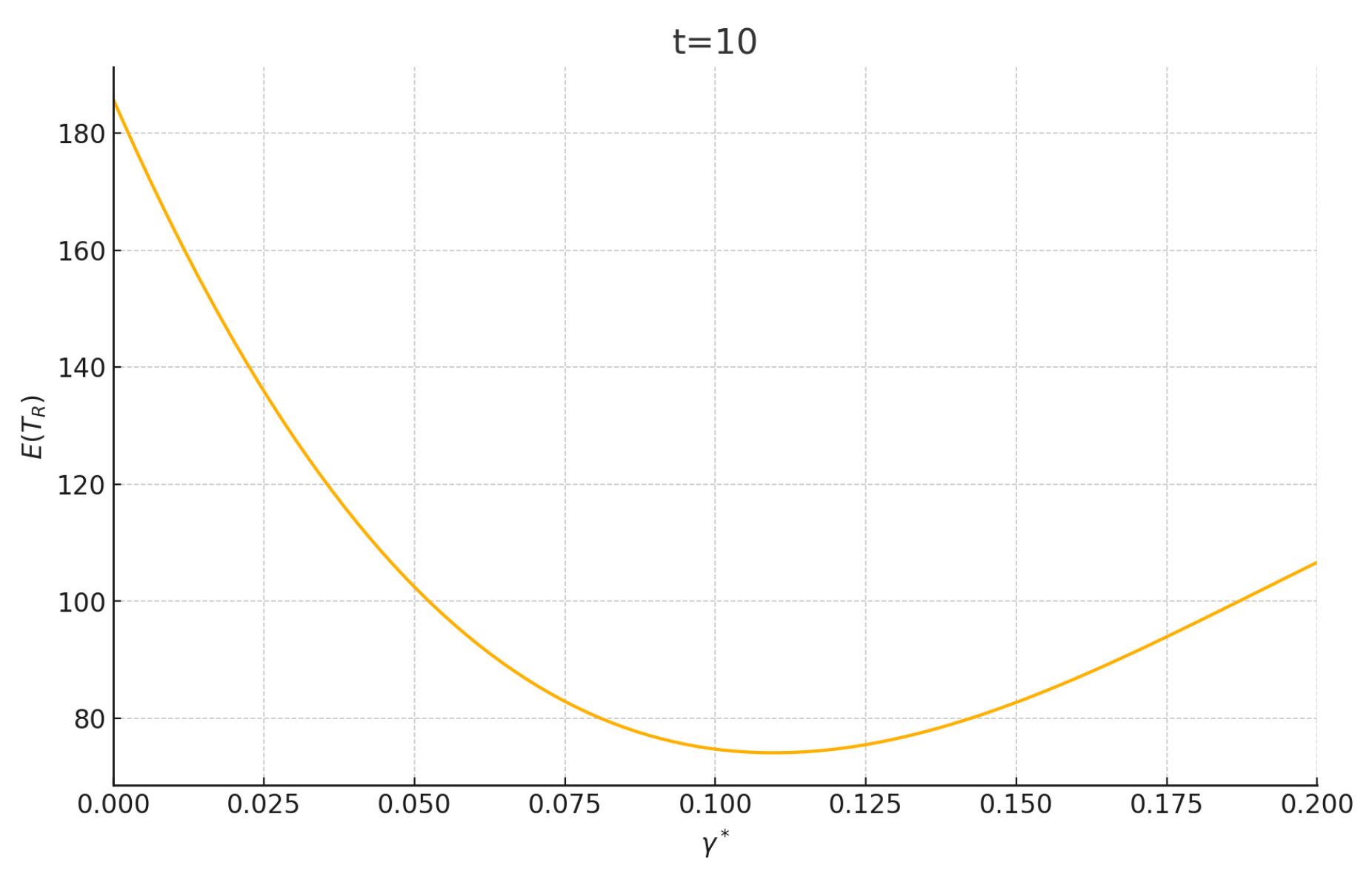
By solving this Equation, we can get the optimal γ * . The plot of γ * vs t see Figure 6. And Figure 7 shows that when t = 10 , the MFPT vs γ on the interval [ 0 , 1 ) .
And by taking the numerical calculations, we find when t , the ratio of the MFPT between the random walk with resetting with the optimal resetting rate and the random walk without resetting:
lim t E ( T O E ( t , γ ) ) γ = γ * E ( T O E ( t ) ) 4 5
So, in this situation, resetting can also improve the efficiency of random search.

5.3. MFPT for Random Walk on T-Fractal with the Resetting Position Selected Randomly

In this section, we discuss the random walk from a random starting node to the fixed node B. In each step, there is probability γ for the walker to reset to the initial position. The starting node is selected according to the stationary distribution, as mentioned in Section III. By solving Equation (28) with the initial condition (29), we get:
Φ T Π B ( t , z ) = 2 t 1 × 3 3 t 2 z 2 + 2 t 1 × 3 3 t 2 z 3 2 t 1 + t 2 ( t + 1 ) 3 t z 2
So, we get:
Φ T Π B ( t , 1 γ ) = 2 t 1 × 3 3 t 2 γ 2 2 t 1 × 3 3 t 2 γ 3 2 t 1 + t 2 ( t + 1 ) 3 t + 4 ( t + 1 ) 3 t γ 2 ( t + 1 ) 3 t γ 2
Therefore, the MFPT under resetting is:
E ( T Π B R ( t ) ) = 1 Φ T Π B ( t , 1 γ ) γ Φ T Π B ( t , 1 γ ) = [ 4 ( t + 1 ) 3 t 2 t 1 × 3 3 t 2 ] γ + 3 2 t 1 + t 2 ( t + 1 ) 3 t 2 t 1 × 3 3 t 2 γ 2 2 t 1 × 3 3 t 2
By taking the first-order derivative of both sides of Equation (57), and setting d d γ E ( T Π B R ( t ) ) = 0 , we get:
[ 4 ( t + 1 ) 3 t 2 t 1 × 3 3 t 2 ] × 2 t 1 × 3 3 t 2 γ 2 + [ 3 2 t 1 + t 2 ( t + 1 ) 3 t ] × 2 t × 3 3 t 2 γ + [ 2 ( t + 1 ) 3 t 3 2 t 1 + t ] × 2 t 1 × 3 3 t 2 = 0
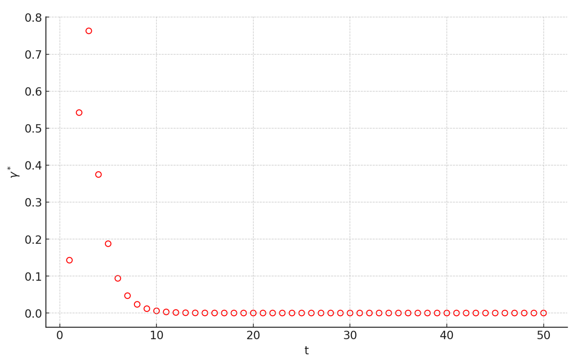
By solving Equation (58), we get the expression for the optimal γ Π B * . And Figure 8 plots the optimal γ Π B * as a function of generation t. We found that from generation 4, the optimal γ Π B * decreases monotonically with the increase of the generation t. And when t , γ Π B * 0 .
By calculating the ratio of MFPT at the optimal resetting rate and the MFPT without resetting, in the T-fractal with a sufficiently large size, we find:
lim t E ( T Π B ( t , γ ) ) γ = γ * E ( T Π B ( t ) ) 0
So, we can conclude that by taking resetting to a randomly drawn from the stationary distribution is a good strategy for the random research. The conclusion in this part provides insights into optimizing research in T-fractal and other large networks.

6. Conclusions

In this study, we explored the dynamics of a random walk on a T-fractal with stochastic resetting, focusing on the effects of resetting on the search efficiency of the random walker. By employing the generating function technique, we established a recursive relation between the generating function of the first passage time (FPT) and derived a connection between the mean first passage time (MFPT) with resetting and the generating function of the FPT without resetting. This analytical framework allowed us to gain deeper insights into how stochastic resetting influences the MFPT.
We examined various scenarios in which a random walker reaches a target site from the starting position, identifying the optimal resetting probability γ * for each case. This optimal γ * minimizes the MFPT, thereby enhancing the efficiency of the search process. Our findings indicate that, compared to the MFPT without resetting, the introduction of a resetting mechanism can significantly improve the search efficiency, especially as the size of the network model increases.
This work demonstrates the potential of stochastic resetting as a valuable strategy for optimizing search processes in complex networks. By minimizing the time to locate a target, resetting can be particularly beneficial in applications where quick and efficient searches are crucial. Our results contribute to the broader understanding of stochastic processes on fractal structures and provide a foundation for further exploration into optimizing search strategies in random environments.
The data that support the findings of this study are available from the corresponding author upon reasonable request.

Author Contributions

For research articles with several authors, a short paragraph specifying their individual contributions must be provided. The following statements should be used “Conceptualization, X.S. and A.L.; methodology, X.S. and A.L.; software, X.S.; validation, F.Z.; formal analysis, A.L.; investigation, X.S.; writing—original draft preparation, X.S.; writing—review and editing, X.S.; visualization, X.S. and S.Z.; supervision, X.S. and S.Z.; project administration, X.S. and F.Z.; funding acquisition, F.Z. All authors have read and agreed to the published version of the manuscript.

Funding

This research was funded by the the Practise Innovation Training Program Projects of Jiangsu University (Grant Y23A117).

Institutional Review Board Statement

Not applicable.

Data Availability Statement

No new data were created or analyzed in this study. Data sharing is not applicable to this article.

Acknowledgments

This work was supported by the Practise Innovation Training Program Projects of Jiangsu University (Grant Y23A117).

Conflicts of Interest

The authors declare no conflict of interest.

Abbreviations

The following abbreviations are used in this manuscript:
MFPT Mean first passage time
FFP First passage probability
FPT First passage time

Appendix A. Some Basic Properties of the Generating Function

Let ξ be a discrete random variable which takes only non-negative integer values. Suppose the probability distribution of the random variable ξ is p n , which means that:
Pr ( ξ = n ) = p n n = 0 , 1 , 2 ,
And the probability generating function of ξ is defined as:
Φ ξ ( z ) = n = 0 p n z n
As shown in the above formula, the generating function is determined by the probability distribution. Therefore, we can infer the probability distribution based on the Taylor expansion of the generating function at z = 0 :
p n = ( n Φ ξ ( z ) / z n ) z = 0 n !
Also, we can derive the mathematical expectation of the random variable ξ , by derivatives of Φ ξ ( z ) calculated at z = 1 :
E ( ξ ) = Φ ξ ( z ) z z = 1
Finally, we list two important properties of the generating function, which are helpful for the calculation of the generating function of the random walk.
If ξ 1 and ξ 2 are two random variables whose generating functions are Φ ξ 1 ( z ) and Φ ξ 2 ( z ) respectively, then the generating function of ξ 1 + ξ 2 is:
Φ ξ 1 + ξ 2 ( z ) = Φ ξ 1 ( z ) Φ ξ 2 ( z )
Let N, ξ 1 , ξ 2 , ⋯ be independent random variables, and ξ i ( i = 1 , 2 , , N ) are identically distributed, the generating function of ξ i are all Φ ξ ( z ) , and the generating function of N is Φ N ( z ) , the random variable S N defined as:
S N = i = 1 N ξ i
Then the generating function of S N is:
Φ S N ( z ) = Φ N ( Φ ξ ( z ) )

Appendix B. The Calculation of the Initial Condition

For a small network, the probability generating function can be calculated directly by using the symbolic toolbox of MATLAB. Here are the general methods to calculate the initial condition.
First, let M = ( P i j ) be the transition matrix of the random walk on the network, where
P i j = 1 d i if i links with j and i isn t in the absorbing domain 0 otherwise
Then, the probability generating function of the matrix M can be obtained by :
Π ( z ) = n = 0 ( z M ) n = ( I z M ) 1
Where I is the identity matrix, and Π ( z ) = ( Φ i j ( z ) ) , where Φ i j ( z ) represents the random walk starting at node i and ends at node j. And Φ i i ( z ) refers to the return time to node i. If j is in the absorbing domain, then Φ i j ( z ) can be referred to as the generating function of the first passage time from i to j. And Φ i i ( z ) refers to the first return time to node i.
In the T-fractal network, in generation 1, we now study the generating function of the first passage time from node A to B, denoted as Φ T A B ( 1 , z ) . First, the transition matrix can be written as (where node B is the absorbing node):
M 1 = 0 0 0 1 0 0 0 0 0 0 0 1 1 3 1 3 1 3 0
Where the nodes A, B, C, O can be denoted by the numbers 1, 2, 3, 4. Then we use MATLAB to calculate Π ( z ) and the generating function of the random walk from A to B is:
Φ T A B ( 1 , z ) = Π ( 1 , 2 ) = z 2 3 2 z 2
Also, we can calculate the generating function from O to B:
Φ T O B ( 1 , z ) = Π ( 4 , 2 ) = z 3 2 z 2
In order to calculate the return time to node B without a trap, we can rewrite the matrix as the situation without a trap:
M 2 = 0 0 0 1 0 0 0 1 0 0 0 1 1 3 1 3 1 3 0
Also, by calculating the Π ( z ) in Equation (A9), we get:
Φ T B B ( 1 , z ) = Π ( 2 , 2 ) = 3 2 z 2 3 ( 1 z 2 )
By the definition of the generating function in Equation (A2), it is obvious that:
Φ T B B ( 0 , z ) = 1 1 z 2
For the following calculation, we define:
Ψ ( z ) = Φ T B B ( 0 , z ) Φ T B B ( 1 , z ) = 3 3 2 z 2
As for generation 2, we can also use the same method to calculate Φ T D E ( 2 , z ) . First, we write the transition matrix of generation 2 where E is the absorbing domain:
M 3 = 0 0 0 1 3 1 3 1 3 0 0 0 0 0 0 0 0 1 0 0 0 0 0 0 0 0 0 0 1 0 0 0 0 0 0 0 0 0 0 1 0 0 0 1 3 1 3 0 0 0 0 0 1 3 0 0 0 0 0 0 0 0 0 0 0 0 1 3 0 0 1 3 0 0 0 0 0 1 3 0 0 0 0 1 0 0 0 0 0 0 0 0 0 0 1 0 0 0 0 0 0 0 0 0 0 1 0 0 0
So, we can derive the initial condition as:
Φ T D E ( 2 , z ) = Π ( 5 , 6 ) = z 2 6 5 z 2
and
Φ T O E ( 2 , z ) = Π ( 1 , 6 ) = z ( 3 2 z 2 ) 6 5 z 2

Appendix C. The Derivation of the Equation (9) (13) (17) in Section III

Let’s first introduce some notations to facilitate our subsequent discussion. First, we denote E ( T A B ( t ) ) as the first moment of the random variable FPT from node A to B in generation t. According to Equation (A4), it is obvious that:
E ( T A B ( 1 ) ) = d d z Φ T A B ( 1 , z ) z = 1 = 6
In the section on the random walk from A to B, we have found the recursion:
Φ T A B ( t , z ) = Φ T A B ( 1 , Φ T A B ( t 1 , z ) )
Now, we take the derivative on both sides of the equation and combine it with Equation (A4), setting z = 1 . We obtain:
E ( T A B ( t ) ) = d d z Φ T A B ( 1 , z ) z = 1 · z Φ T A B ( t 1 , z ) z = 1 = ( E ( T A B ( 1 ) ) ) t = 6 t
As to the random walk from D to E, the recursion is:
Φ T D E ( t , z ) = Φ T D E ( 2 , Φ T A B ( t 2 , z ) )
We can also take the derivative on both sides as the same method, we get:
E ( T D E ( t ) ) = d d z Φ T D E ( 2 , z ) z = 1 · z Φ T A B ( t 2 , z ) z = 1 = 2 · 6 t 1
For the random walk from O to B, the recursion is:
Φ T O B ( t , z ) = Φ T O B ( 1 , Φ T A B ( t 1 , z ) )
Using the same method, we can obtain:
E ( T O B ( t ) ) = d d z Φ T O B ( 1 , z ) z = 1 · z Φ T A B ( t 1 , z ) z = 1 = 5 · 6 t 1
E ( T O E ( t ) ) = d d z Φ T O E ( 2 , z ) z = 1 · z Φ T A B ( t 2 , z ) z = 1 = 7 · 6 t 2

Appendix D. The derivation of the Equation (25) (26)

Due to the symmetry of the network, the outermost nodes (such as A,B,C, see in Figure 2) are topologically equivalent. So without lose of generality, we only consider the return time for B. We denote T B B ( t ) the return time of B in generation t of the T-fractal (notice that this may not be the first return time). And we denote Φ T B B ( t , z ) the generating function of T B B ( t ) . Similar to the method used in Section III, we first consider an arbitrary path which starts from B and ends at B in generation t of T-fractal. It can be written as:
π = ( v 0 = B , v 1 , v 2 , , v T B B ( t ) = B )
Where v i is the node where the walker reaches at time i. And let Ω = { A , B } , the node generated in generation 0. Similar to the approach in Section III, we can obtain a simplified path whose nodes were in Ω :
σ ( π ) = ( v τ 0 = B , v τ 1 , , v N = B )
Where v τ i Ω and N stands for the return time for B on T-fractal in generation 0. So, the generating function of N is Φ T B B ( 0 , z ) . For any return path of B, maybe v τ N is not the last node in path π . That is to say, after v τ N , there may be a sub-path from B to B, which does not reach node A. We can regard this as the return time of B with the trap (or absorbing domain) A. We denote its length by T B B ( t ) in generation t of T-fractal. And the generating function of the random variable T B B ( t ) denote as Φ T B B ( t , z ) . Let T i = τ i τ i 1 denote the interval time between random walk in Ω , so we have:
T B B ( t ) = T 1 + T 2 + + T N + T B B ( t )
Here, T i ( i = 1 , 2 , , N ) are independent identically distributed random variables, each of them stands for the random walk from A to B (or B to A) in generation t of the T-fractal. So the generating function of the T i is Φ T A B ( t , z ) . So by the property of the generating function (A5) (A7), the generating function of T B B ( t ) can be written as:
Φ T B B ( t , z ) = Φ T B B ( 0 , Φ T A B ( t , z ) ) × Φ T B B ( t , z )
For the random variable T B B ( t ) , we set Ω = { A , B , C , O } , and T i stands for the interval time between the random walk in set Ω , it can be used the same method to derive:
T B B ( t ) = T 1 + T 2 + + T N + T B B ( t 1 )
The generating function of T i is Φ T A B ( t 1 , z ) , and the generating function of the random variable N is Φ T B B ( 1 , z ) . Due to the independence of the random variable T i ( i = 1 , 2 , , N ) and T B B ( t 1 ) , we have:
Φ T B B ( t , z ) = Φ T B B ( 1 , Φ T A B ( t 1 , z ) ) × Φ T B B ( t 1 , z )
Replacing Φ T B B ( t , z ) and Φ T A B ( t , z ) in Equation (A33) respectively to Equation (A31), we get the recurrence for Φ T B B ( t , z ) and can be simplified as:
Φ T B B ( t , z ) = Φ T B B ( t 1 , z ) Ψ ( Φ T A B ( t , z ) )
Where
Ψ ( z ) = Φ T B B ( 0 , z ) Φ T B B ( 1 , z )
Which is also the Equation (25) and (26).

References

  1. J. R. Norris, Markov chains. Cambridge university press, 1998, no. 2.
  2. C. Borgs, J. T. Chayes, A. Frieze, J. H. Kim, P. Tetali, E. Vigoda et al., “Torpid mixing of some monte carlo markov chain algorithms in statistical physics,” in 40th Annual Symposium on Foundations of Computer Science (Cat. No. 99CB37039). IEEE, 1999, pp. 218–229.
  3. A. Krogh, M. Brown, I. S. Mian, K. Sjölander, and D. Haussler, “Hidden markov models in computational biology: Applications to protein modeling,” Journal of molecular biology, vol. 235, no. 5, pp. 1501–1531, 1994.
  4. B.-J. Yoon, X. Qian, and S. M. E. Sahraeian, “Comparative analysis of biological networks: Hidden markov model and markov chain-based approach,” IEEE Signal Processing Magazine, vol. 29, no. 1, pp. 22–34, 2011.
  5. D. S. Myers, L. Wallin, and P. Wikström, “An introduction to markov chains and their applications within finance,” MVE220 Financial Risk: Reading Project, vol. 26, 2017.
  6. G. Bolch, S. Greiner, H. De Meer, and K. S. Trivedi, Queueing networks and Markov chains: modeling and performance evaluation with computer science applications. John Wiley & Sons, 2006.
  7. A. H. Gandjbakhche and G. H. Weiss, “V: Random walk and diffusion-like models of photon migration in turbid media,” Progress in optics, vol. 34, pp. 333–402, 1995.
  8. E. F. Fama, “Random walks in stock market prices,” Financial analysts journal, vol. 51, no. 1, pp. 75–80, 1995.
  9. B. C. Nolting, Random search models of foraging behavior: Theory, simulation, and observation. The University of Nebraska-Lincoln, 2013.
  10. C. Hall, “The simulation of particle motion in the atmosphere by a numerical random-walk model,” Quarterly Journal of the Royal Meteorological Society, vol. 101, no. 428, pp. 235–244, 1975.
  11. M. Kac, “Random walk and the theory of brownian motion,” The American Mathematical Monthly, vol. 54, no. 7P1, pp. 369–391, 1947.
  12. E. F. Fama, “Efficient capital markets,” Journal of finance, vol. 25, no. 2, pp. 383–417, 1970.
  13. H. C. Berg and D. A. Brown, “Chemotaxis in escherichia coli analysed by three-dimensional tracking,” nature, vol. 239, no. 5374, pp. 500–504, 1972.
  14. R. Motwani and P. Raghavan, Randomized algorithms. Cambridge university press, 1995.
  15. Y. Chen, Z. Yuan, L. Gao, and J. Peng, “Optimizing search processes with stochastic resetting on the pseudofractal scale-free web,” Physical Review E, vol. 108, no. 6, p. 064109, 2023.
  16. O. Blumer, S. Reuveni, and B. Hirshberg, “Stochastic resetting for enhanced sampling,” The journal of physical chemistry letters, vol. 13, no. 48, pp. 11 230–11 236, 2022.
  17. M. R. Evans and S. N. Majumdar, “Diffusion with stochastic resetting,” Physical review letters, vol. 106, no. 16, p. 160601, 2011.
  18. M. A. Lomholt, L. Lizana, R. Metzler, and T. Ambjörnsson, “Microscopic origin of the logarithmic time evolution<? format?> of aging processes in complex systems,” Physical review letters, vol. 110, no. 20, p. 208301, 2013.
  19. S. N. Majumdar, S. Sabhapandit, and G. Schehr, “Random walk with random resetting to the maximum position,” Physical Review E, vol. 92, no. 5, p. 052126, 2015.
  20. E. Raposo, S. Buldyrev, M. Da Luz, G. Viswanathan, and H. Stanley, “Lévy flights and random searches,” Journal of Physics A: mathematical and theoretical, vol. 42, no. 43, p. 434003, 2009.
  21. A. Chechkin and I. M. Sokolov, “Random search with resetting: a unified renewal approach,” Physical review letters, vol. 121, no. 5, p. 050601, 2018.
  22. R. D. Schumm, “Analytical and monte carlo methods for stochastic search processes with partially reactive domains,” Ph.D. dissertation, The University of Utah, 2023.
  23. S. Redner, A guide to first-passage processes. Cambridge university press, 2001.
  24. V. Balakrishnan, “Random walks on fractals,” Materials Science and Engineering: B, vol. 32, no. 3, pp. 201–210, 1995.
  25. S. Goldstein, “Random walks and diffusions on fractals,” Percolation theory and ergodic theory of infinite particle systems, pp. 121–129, 1987.
  26. Y. Lin, B. Wu, and Z. Zhang, “Determining mean first-passage time on a class of treelike regular fractals,” Physical Review E—Statistical, Nonlinear, and Soft Matter Physics, vol. 82, no. 3, p. 031140, 2010.
  27. J. Peng, R. Shao, L. Chen, and H. E. Stanley, “Moments of global first passage time and first return time on tree-like fractals,” Journal of Statistical Mechanics: Theory and Experiment, vol. 2018, no. 9, p. 093205, 2018.
  28. O. L. Bonomo and A. Pal, “The p∖’{o} lya and sisyphus lattice random walks with resetting–a first passage under restart approach,” arXiv preprint arXiv:2106.14036, 2021.
  29. ——, “First passage under restart for discrete space and time: application to one-dimensional confined lattice random walks,” Physical Review E, vol. 103, no. 5, p. 052129, 2021.
  30. S. Hwang, D.-S. Lee, and B. Kahng, “First passage time for random walks in heterogeneous networks,” Physical review letters, vol. 109, no. 8, p. 088701, 2012.
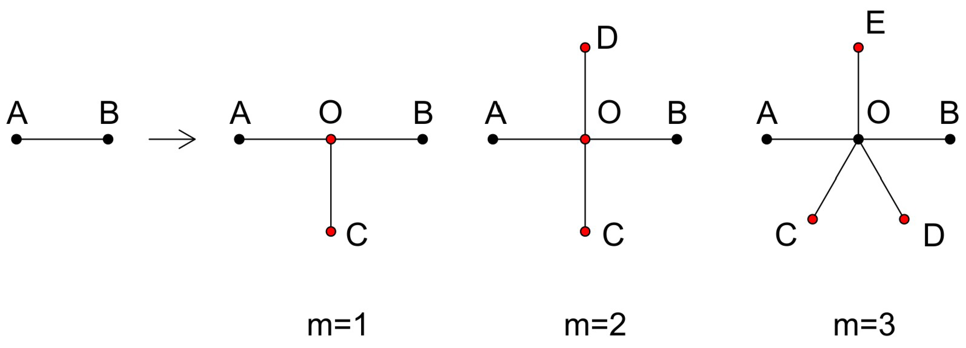
Figure 1. Iterative construction of the tree-like fractals from generation 0 to generation 1. The next generation was created by adding one vertex O between node A and B, then add m edges to O.
Preprints 122030 g001
Figure 2. The growing process for the T-fractal(a special case about tree-like fractals when m=1). The nodes with black colors were generated in generation 0, while red nodes in generation 1, blue nodes in generation 2, green nodes in generation 3 and so on.
Preprints 122030 g002
Figure 3. Another approach to obtain the tree-like fractal. F t can be regarded as m + 2 copies of F t 1 , connecting the outermost vertex and the innermost vertex.
Preprints 122030 g003
Figure 4. Plot of the optimal resetting probability γ O B * as a function of t. From t = 20, the γ * decreases, and from t = 27, γ * increase again. And when t , γ * 0 . 41 .
Preprints 122030 g004
Figure 5. Plot of the E ( T R ) vs γ when t = 30 , the optimal γ * is around 0.40 where the MFPT reaches its minimum.
Preprints 122030 g005
Figure 6. Plot of the optimal resetting probability γ O E * as a function of t. The γ O E * decreases from generation 7, and when t , γ O E * 0 .
Preprints 122030 g006
Figure 7. Plot of the MFPT of generation 10 as a function of γ , the optimal γ * is about 0.11 where the MFPT reaches its minimum.
Preprints 122030 g007
Figure 8. Plot of the optimal resetting probability γ Π B * as a function of t. The γ Π B * decreases from generation 3, and when t , γ Π B * 0 .
Preprints 122030 g008
Disclaimer/Publisher’s Note: The statements, opinions and data contained in all publications are solely those of the individual author(s) and contributor(s) and not of MDPI and/or the editor(s). MDPI and/or the editor(s) disclaim responsibility for any injury to people or property resulting from any ideas, methods, instructions or products referred to in the content.
Copyright: This open access article is published under a Creative Commons CC BY 4.0 license, which permit the free download, distribution, and reuse, provided that the author and preprint are cited in any reuse.
Alerts
Prerpints.org logo

Preprints.org is a free preprint server supported by MDPI in Basel, Switzerland.

Subscribe

© 2025 MDPI (Basel, Switzerland) unless otherwise stated