Compartmental Description of the Cosmological Baryonic Matter Cycle. II. Inclusion of Triggered Star Formation

Preprint

Article

Compartmental Description of the Cosmological Baryonic Matter Cycle. II. Inclusion of Triggered Star Formation

This version is not peer-reviewed.

Martin Kröger^*

Reinhard Schlickeiser^*

Martin Kröger^*

Reinhard Schlickeiser^*

This version is not peer-reviewed.

Altmetrics

Downloads

Views

Comments

Submitted:

18 October 2024

Posted:

24 October 2024

You are already at the latest version

Abstract

Context: The earlier introduced compartmental description, well-known from the description of infection diseases and epidemics, was applied here to describe the nonlinear temporal evolution of the baryonic matter in interstellar gas and stars in the presence of triggered star formation. Aims: The competition of triggered star formation, spontaneous star formation, stellar feedback and stellar evolution was theoretically investigated to understand the baryonic matter cycle including luminous baryonic matter in main-sequence stars and weakly luminous matter in white dwarfs, neutron stars and black holes. Of particular interest was the understanding of the cosmic star formation history and the redshift dependence of the gas and stellar fractions using compartmental models. Methods: For stationary rates of spontaneous and triggered star formation, continuous stellar feedback and stellar evolution exact and approximate analytical solutions of the time evolution of the fractions of stellar and locked-in stellar matter were derived involving the time dependence of the gaseous fraction G(t). The high accuracy of the analytical solutions is proven by comparison with the exact numerical solutions of the GSL equations. Results: The inclusion of the triggered star formation process explains the observed cosmological star formation rate, the integrated stellar density at redshifts below z=8, and the present-day gas and stellar fractions very well. The generalized GSL-model provides excellent fits to the observed redshift dependencies of the star formation rate and the integrated stellar density. Moreover, it explains the observed present-day gas and stellar fractions, and it makes predictions on the future evolution of these fractions in the universe.

Keywords:

Subject:

Physical Sciences - Astronomy and Astrophysics

1. Introduction

Recently ([1] - hereafter referred to as part I) the compartmental description, well-known from the description of infection diseases and epidemics, has been introduced to describe the temporal evolution of the baryonic matter in interstellar gas and stars. Such a description makes use of gaseous and stellar fractions of the total baryonic matter and transition rates between these fractions. In particular, the respective rates of spontaneous (

β (t) G (t)

) and triggered (

a (t) S (t) G (t)

) star formation regulate the transfer

G (t) \to S (t)

from gas to luminous main-sequence stars, whereas the stellar feedback rate (

b (t) S (t)

) determines the feedback

S (t) \to G (t)

from luminous stars to gas. Thirdly the stellar evolution rate (

c (t) S (t)

) regulates the transfer

S (t) \to L (t)

from luminous stars to locked-in stellar matter in the form of white dwarfs, neutron stars and black holes which are much less luminous and have no significant stellar feedback to the gaseous matter compartment.

In part I the process of triggered star formation has been ignored and the resulting exact analytical solutions for stationary rates of spontaneous formation, feedback and evolution have been compared with the observed cosmological star formation rate and the integrated stellar density. It has been demonstrated that the simplified GS-model ignoring stellar evolution cannot explain the observations. The comparison of the full gas-stars-locked-in (GSL) model including stellar evolution is more favorable but still far from being perfect. The non-perfect agreement of the GSL-model with only spontaneous star formation process therefore is a strong motivation to investigate the role of the additional triggered star formation process, which is the subject of the present part II.

Here, the competition of triggered and spontaneous star formation, stellar feedback and stellar evolution was theoretically investigated with analytical and numerical solutions of the nonlinear dynamical GSL equations. Following part I, baryonic matter exists as interstellar and intergalactic gas with the fraction

G (t)

and in two forms of stellar matter:

S (t)

denotes the fraction of luminous stellar matter in main-sequence stars while

L (t)

refers to the fraction of weakly luminous matter in white dwarfs, neutron stars and black holes (referred to as locked-in matter) which have no significant stellar feedback to the gaseous matter compartment. The temporal evolution of the three fractions is controlled by the respective rates of spontaneous star formation (

β (t) G (t)

) and of triggered star formation (

a (t) G (t) S (t)

of gas to stellar matter, of stellar feedback (

b (t) S (t)

) of stellar to gaseous matter, and of the formation (

c (t) S (t)

) of white dwarfs, neutron stars and black holes from stellar evolution. Obviously, the inclusion of triggered star formation introduces a nonlinearity in the GSL equations as it is depends on the product

G (t) S (t)

The organization of this manuscript is as follows. The GSL-compartmental model for the baryonic matter cycle is revisited in Section 2. While Section 3 is concerned with the GS-limit for negligible stellar evolution, the full GSL model for stationary ratios is investigated in Section 4. Having obtained general relationships between the compartments, and their limiting, stationary values, approximate solutions are derived and tested in Section 5. Section 6 connects the GSL fractions with the cosmic star formation history and discusses observational constraints that help us identifying the parameters of the GSL model. The resulting redshift dependency of the gas and stellar fractions is presented in Section 7. A summary and conclusions are provided in Section 8.

2. GSL-Compartmental Model for the Baryonic Matter Cycle

As in part I we considered the total system of matter either in stars or in interstellar gas and introduce the compartments G (gas), S (stars) and L (locked-in matter in white dwarfs, neutron stars and black holes) where

G (t)

S (t)

and

L (t)

denote the relative fractions of luminous matter in the three compartments, respectively, as a function of time t.

2.1. Starting Equations

The three fractions obey the sum constraint

G (t) + S (t) + L (t) = 1,

(1)

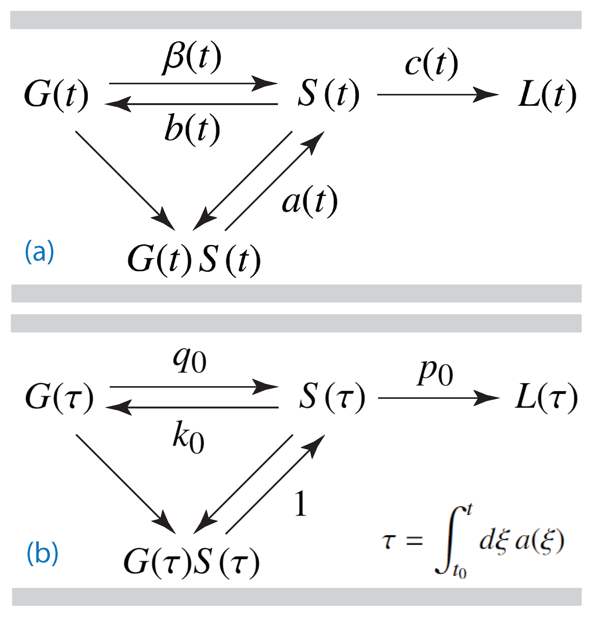
holding at all times t after the begin of the baryonic evolution at time

t = t_{0}

. The dynamical evolution of the three fractions is described by the nonlinear dynamical GSL equations (Figure 1)

\begin{matrix} \frac{d G}{d t} & = & - a (t) G (t) S (t) - β (t) G (t) + b (t) S (t), \end{matrix}

(2)

\begin{matrix} \frac{d S}{d t} & = & a (t) G (t) S (t) + β (t) G (t) - b (t) S (t) - c (t) S (t), \end{matrix}

(3)

and

\frac{d L}{d t} = c (t) S (t),

(4)

respectively. As initial condition in the presence of spontaneous star formation (

β (t) > 0

) we adopted

G (t_{0}) = 1, S (t_{0}) = 0, L (t_{0}) = 0 .

(5)

As an aside we note that in the absence of spontaneous star formation (

β = 0

) the initial conditions (5) had to be modified to

G (t_{0}) = 1 - η

S (t_{0}) = η

L (t_{0}) = 0

, with the small initial stellar fraction

η ≪ 1

. Without a finite albeit tiny initial fraction the process of triggered star formation does not start. The initial time

t_{0}

corresponds to the redshift

z = 1100

Of particular interest is the formation rate

\overset{˚}{J} (t)

of new stars as a function of time,

\overset{˚}{J} (t) = a (t) G (t) S (t) + β (t) G (t) .

(6)

The first term represents the rate from triggered star formation, whereas the second term is the rate from spontaneous star formation.

In contrast to part I we included in the analysis also the process of triggered star formation which is nonlinear as it depends on the product

G (t) S (t)

. Exact and approximate analytical solutions of the dynamical equations of the GSL-model (1)–(5) were derived which hold for stationary rates as well as for the case of the same time dependency of all rates.

2.2. Stationary Ratios

We here introduced the three ratios

k (t) = \frac{b (t)}{a (t)}, q (t) = \frac{β (t)}{a (t)}, p (t) = \frac{c (t)}{a (t)},

(7)

indicating the strength of stellar feedback, spontaneous star formation and stellar evolution with respect to triggered star formation, respectively.

For ease of exposition we considered, similar to part I, the case of stationary ratios

k (τ) = k_{0} =

const,

q (τ) = q_{0} =

const, and

p (τ) = p_{0} =

const, as shown in Figure 1. This case applies to stationary values of the rates

a (t) = a_{0}

b (t) = b_{0}

β = β_{0}

and

c (t) = c_{0}

as well as to any time-dependent star formation rate

a (t)

, provided

b (t) \propto a (t)

β (t) \propto a (t)

, and

c (t) \propto a (t)

have the same time variation while their absolute values can be different.

It is appropriate to introduce the dimensionless reduced time variable

τ = \int_{t_{0}}^{t} d ξ a (ξ) = a_{0} (t - t_{0})

(8)

in terms of the stationary triggered star formation rate

a_{0}

. This reduced time scale differs from the one introduced in part I:

\tilde{t} = β_{0} (t - t_{0})

. Obviously for stationary rates the relation

τ = \frac{a_{0}}{β_{0}} \tilde{t}

(9)

holds. In a flat

Λ

CDM Friedmann cosmology with

Ω_{m} = 0.3

and the Hubble constant

H_{0} = 70 h_{70}

km^s−1 Mpc^s−1 the relation (9) implies with Equations (I-42)1 the redshift dependency (for details see Appendix A)

\begin{matrix} τ (z) & ≃ & \frac{ϕ (z)}{{(1 + z)}^{3 / 2}}, ϕ (z) = ϕ ζ (z), ϕ = \frac{5.37 {\tilde{a}}_{0}}{h_{70}}, \end{matrix}

(10)

\begin{matrix} ζ (z) & = & \frac{{(1 + z)}^{3 / 2}}{\sqrt{\frac{7}{3} + {(1 + z)}^{3}}} ≃ 1 - (1 - \sqrt{\frac{3}{10}}) e^{- 4 z / 3}, \end{matrix}

(11)

\begin{matrix} ζ (0) & = & \sqrt{0.3} = 0.548, \end{matrix}

(12)

In the following the modification introduced by the factor (11) entered only Section 7 to calculate the present-day quantities at redshift

z = 0

whereas for finite redshift we set

ζ (z) = 1

. In Equation (10) the triggered star formation rate is scaled as

a_{0} = 10^{- 17} {\tilde{a}}_{0} Hz .

(13)

The Equations (1)–(4) then read

\begin{matrix} \frac{d G}{d τ} & = & - G (τ) S (τ) - q_{0} G (τ) + k_{0} S (τ), \end{matrix}

(14a)

\begin{matrix} \frac{d S}{d τ} & = & G (τ) S (τ) + q_{0} G (τ) - [k_{0} + p_{0}] S (τ), \end{matrix}

(14b)

\begin{matrix} \frac{d L}{d τ} & = & p_{0} S (τ), \end{matrix}

(14c)

\begin{matrix} 1 & = & G (τ) + S (τ) + L (τ), \end{matrix}

(14d)

obeying the initial conditions

G (τ = 0) = 1, S (τ = 0) = 0, L (τ = 0) = 0 .

(15)

In Equations (14) we introduced the dimensionless constant ratios

k_{0} = \frac{b_{0}}{a_{0}}, q_{0} = \frac{β_{0}}{a_{0}}, p_{0} = \frac{c_{0}}{a_{0}} .

(16)

The formation rate of new stars (6) as a function of reduced time is given by

j (τ) = G (τ) S (τ) + q_{0} G (τ) .

(17)

τ = \infty

Equation (14) attain a stationary state where all time derivatives vanish. For finite

p_{0} > 0

Equation (14c) then implies

S_{\infty} = 0

, so that

G_{\infty} = 0

according to Equation (14a) leading to

L (\infty) = 1

according to the sum constraint (14d). For later use we thus note

G_{\infty} = S_{\infty} = 0, L (\infty) = 1

(18)

Equation (14) could be simplified upon introducing

M (τ) = G (τ) - k_{0}, N (τ) = S (τ) + q_{0} .

(19)

Using

M (τ)

and

N (τ)

yielded for Equations (14)

\begin{matrix} \frac{d M}{d τ} & = & - M (τ) N (τ) - q_{0} k_{0}, \end{matrix}

(20a)

\begin{matrix} \frac{d N}{d τ} & = & M (τ) N (τ) + q_{0} k_{0} - p_{0} [N (τ) - q_{0}], \end{matrix}

(20b)

\begin{matrix} \frac{d L}{d τ} & = & p_{0} [N (τ) - q_{0}], \end{matrix}

(20c)

\begin{matrix} 1 & = & M (τ) + N (τ) + L (τ) + k_{0} - q_{0}, \end{matrix}

(20d)

with the initial conditions

M (τ = 0) = 1 - k_{0}, N (τ = 0) = q_{0}, L (τ = 0) = 0 .

(21)

In the following two sections we investigated analytical solutions of Equations (14)–(21): first, for the special GS-case of negligible stellar evolution (

c_{0} = p_{0} = 0

) in Section 3, before we investigated the general GSL-case (Section 4).

3. GS-Limit for Negligible Stellar Evolution

In the case of vanishing stellar evolution,

c_{0} = p_{0} = 0

, implying

L (τ) = 0

at all times (Figure 1). In that case the reduced GSL model Equations (14a)–(14b) and (14d) simplified to the GS model equation

\begin{matrix} \frac{d G}{d τ} & = & - G (τ) S (τ) - q_{0} G (τ) + k_{0} S (τ), \end{matrix}

(22a)

\begin{matrix} \frac{d S}{d τ} & = & G (τ) S (τ) + q_{0} G (τ) - k_{0} S (τ), \end{matrix}

(22b)

\begin{matrix} 1 & = & G (τ) + S (τ), \end{matrix}

(22c)

so that with Equations (19) we obtained

\begin{matrix} \frac{d M}{d τ} & = & - M (τ) N (τ) - q_{0} k_{0}, \end{matrix}

(23a)

\begin{matrix} \frac{d N}{d τ} & = & M (τ) N (τ) + q_{0} k_{0} . \end{matrix}

(23b)

Equation (23a) readily provided

N (τ) = - \frac{\frac{d M}{d τ} + k_{0} q_{0}}{M (τ)},

(24)

so that

S (τ) = - q_{0} - \frac{\frac{d (G (τ) - k_{0})}{d τ} + k_{0} q_{0}}{G (τ) - k_{0}} = - q_{0} - \frac{\frac{d G (τ)}{d τ} + k_{0} q_{0}}{G (τ) - k_{0}} .

(25)

Upon insertion of Equation (25) the sum constraint (22c) became

1 + q_{0} = G (τ) - \frac{\frac{d G (τ)}{d τ} + k_{0} q_{0}}{G (τ) - k_{0}},

(26)

or equivalently,

\frac{d G (τ)}{d τ} = G^{2} (τ) - (1 + q_{0} + k_{0}) G (τ) + k_{0} .

(27)

According to Equation (27) the fraction

G (τ)

approaches a stationary value

G_{\infty}

τ \to \infty

, which is given by

\begin{matrix} G_{\infty} & = & \frac{1}{2} (χ_{0} - ω_{0}) \\ = & \frac{1}{2} [1 + q_{0} + k_{0} - \sqrt{{(1 + q_{0})}^{2} + k_{0}^{2} - 2 k_{0} (1 - q_{0})}], \end{matrix}

(28)

where

χ_{0} \equiv 1 + k_{0} + q_{0} > 1, ω_{0} \equiv \sqrt{χ_{0}^{2} - 4 k_{0}} \geq 0 .

(29)

Taking into account the initial conditions (15), the solution of Equation (27) could be written as

\begin{matrix} τ & = & \int_{1}^{G (τ)} \frac{d x}{x^{2} - (1 + q_{0} + k_{0}) x + k_{0}} \\ = & - \int_{1}^{G (τ)} \frac{d x}{(x - G_{\infty}) (χ_{0} - G_{\infty} - x)} \\ = & - \int_{1 - G_{\infty}}^{G (τ) - G_{\infty}} \frac{d y}{y (χ_{0} - 2 G_{\infty} - y)} \\ = & - \frac{1}{ω_{0}} \int_{1 - G_{\infty}}^{G (τ) - G_{\infty}} d y [\frac{1}{y} + \frac{1}{ω_{0} - y}] . \end{matrix}

(30)

This integral evaluated to

\begin{matrix} ω_{0} τ & = & - {[ln \frac{y}{ω_{0} - y}]}_{1 - G_{\infty}}^{G - G_{\infty}} = {[ln (\frac{ω_{0}}{y} - 1)]}_{1 - G_{\infty}}^{G - G_{\infty}} \\ = & ln \frac{\frac{ω_{0}}{G - G_{\infty}} - 1}{\frac{ω_{0}}{1 - G_{\infty}} - 1}, \end{matrix}

(31)

or equivalently

G (τ) = G_{\infty} + \frac{ω_{0}}{1 + (\frac{ω_{0}}{1 - G_{\infty}} - 1) e^{ω_{0} τ}} .

(32)

The sum constraint (22c) then readily yielded

S (τ) = 1 - G (τ) = 1 - G_{\infty} - \frac{ω_{0}}{1 + (\frac{ω_{0}}{1 - G_{\infty}} - 1) e^{ω_{0} τ}},

(33)

providing

\begin{matrix} S_{\infty} & = & 1 - G_{\infty} \\ = & \frac{1}{2} [1 - q_{0} - k_{0} + \sqrt{{(1 + q_{0})}^{2} + k_{0}^{2} - 2 k_{0} (1 - q_{0})}] . \end{matrix}

(34)

Consequently, the dimensionless star formation rate (17) became

\begin{matrix} j (τ) & = & G (τ) [S (τ) + q_{0}] = [G_{\infty} + \frac{ω_{0}}{1 + (\frac{ω_{0}}{1 - G_{\infty}} - 1) e^{ω_{0} τ}}] \times \\ [1 + q_{0} - G_{\infty} - \frac{ω_{0}}{1 + (\frac{ω_{0}}{1 - G_{\infty}} - 1) e^{ω_{0} τ}}] \end{matrix}

(35)

where we recall that

ω_{0}

and

G_{\infty}

are both known in terms of

k_{0}

and

q_{0}

. The maximum of

j (τ)

is attained at

τ_{j}

solving

d j (τ) / d τ = 0

. This yielded the dimensionless peak time

τ_{j} = \frac{1}{ω_{0}} ln [\frac{1 + q_{0} - 2 (G_{\infty} + ω_{0})}{(\frac{ω_{0}}{1 - G_{\infty}} - 1) (2 G_{\infty} - q_{0} - 1)}],

(36)

as well, upon inserting

τ_{j}

into Equation (28), the peak amplitude

j_{\max} = \frac{{(1 + q_{0})}^{2}}{4},

(37)

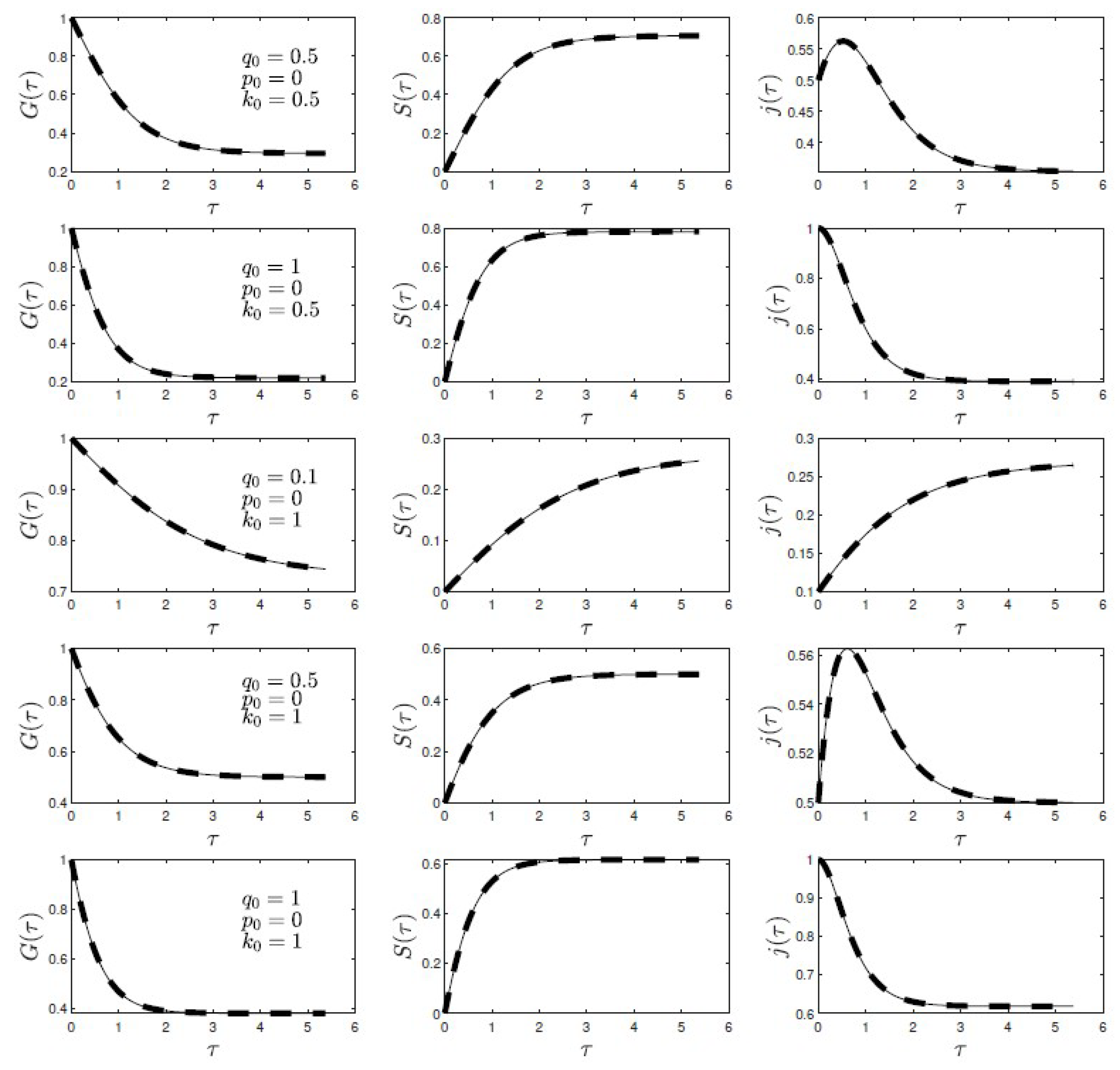
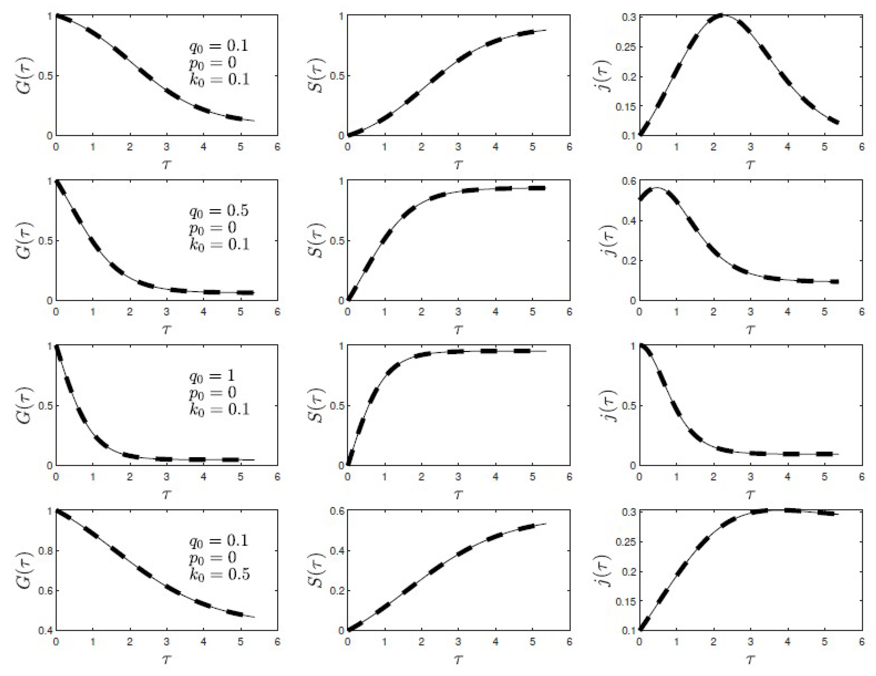
where we made use of the definitions of

χ_{0}

ω_{0}

, and

G_{\infty}

according to Equation (28) to simplify the final expression. For the present case of

p_{0} = 0

the analytical solutions (32), (33), (28) are shown to be identical with the numerical solution in Figure for various choices of

q_{0}

and

k_{0}

. Following [2] the numerical solution of the GSL equations we obtained using the 10th order predictor–corrector Adams method ([3,4]). Within 0.1% precision, a single-step solver based on a modified Rosenbrock formula of order 2, implemented by [5] as ode23s in Matlab^TM yielded practically indistinguishable results. The excellent agreement between the numerical and analytical solutions in Figure confirms the validity of our derivations.

4. The Full GSL Model for Stationary Ratios

4.1. Further Reduction

For the full GSL-model including stellar evolution

p_{0} > 0

we first reduced Equations (14) further. Equation (20a) readily yielded

N (τ) = - \frac{\frac{d M (τ)}{d τ} + q_{0} k_{0}}{M (τ)},

(38)

and Equation (20b) could be written as

\begin{matrix} p_{0} & = & M (τ) + \frac{q_{0} (k_{0} + p_{0})}{N (τ)} - \frac{d ln N (τ)}{d τ} . \end{matrix}

(39)

Substituting

N (τ) = q_{0} (k_{0} + p_{0}) X (τ)

(40)

the Equation (39) reads

p_{0} - M (τ) = \frac{1}{X (τ)} - \frac{d ln X (τ)}{d τ} = \frac{1}{X (τ)} [1 - \frac{d X (τ)}{d τ}],

(41)

or equivalently,

\frac{d X (τ)}{d τ} + [p_{0} - M (τ)] X (τ) = 1 .

(42)

This last Equation (42) was readily solved by

X (τ) = [c_{0} + \int_{0}^{τ} d x e^{p_{0} x - \int_{0}^{x} d τ^{'} M (τ^{'})}] e^{- p_{0} τ + \int_{0}^{τ} d τ^{'} M (τ^{'})}

(43)

with the integration constant

c_{0} = X (0)

. The solution (43) implied

N (τ) = q_{0} (k_{0} + p_{0}) [c_{0} + \int_{0}^{τ} d x e^{p_{0} x - \int_{0}^{x} d τ^{'} M (τ^{'})}] e^{- p_{0} τ + \int_{0}^{τ} d τ^{'} M (τ^{'})} .

(44)

The initial value

N (τ = 0) = q_{0}

then provided

c_{0} = 1 / (k_{0} + p_{0})

, so that

\begin{matrix} S (τ) & = & N (τ) - q_{0} \\ = & q_{0} [1 + (k_{0} + p_{0}) \int_{0}^{τ} d x e^{- U (x)}] e^{U (τ)} - q_{0}, \end{matrix}

(45)

where we introduced

U (τ) = \int_{0}^{τ} d τ^{'} M (τ^{'}) - p_{0} τ,

(46)

implying

\begin{matrix} M (τ) & = & G (τ) - k_{0} = \frac{d U (τ)}{d τ} + p_{0}, \\ \frac{d M (τ)}{d τ} & = & \frac{d G (τ)}{d τ} = \frac{d^{2} U (τ)}{d τ^{2}}, \end{matrix}

(47)

with

\begin{matrix} U (0) & = & 0, U^{''} (0) = G^{'} (0) = - q_{0}, \\ U^{'} (0) & = & G (0) - k_{0} - p_{0} = 1 - k_{0} - p_{0} . \end{matrix}

(48)

Inserting Equations (45) and (47) yielded for Equation (38)

\begin{matrix} - q_{0} k_{0} & = & \frac{d^{2} U}{d τ^{2}} + q_{0} [\frac{d U (τ)}{d τ} + p_{0}] e^{U (τ)} \times \\ [1 + (k_{0} + p_{0}) \int_{0}^{τ} d x e^{- U (x)}] . \end{matrix}

(49)

With

\frac{d U (τ)}{d τ} e^{U (τ)} = \frac{d}{d τ} e^{U (τ)},

(50)

and

\frac{d e^{U (τ)}}{d τ} \int_{0}^{τ} d x e^{- U (x)} = \frac{d}{d τ} [e^{U (τ)} \int_{0}^{τ} d x e^{- U (x)}] - 1

(51)

the Equation (49) could be further reduced to

\frac{d}{d τ} [\frac{d U (τ)}{d τ} + q_{0} e^{U (τ)} (1 + (k_{0} + p_{0}) \int_{0}^{τ} d x e^{- U (x)})]

= q_{0} p_{0} [1 - e^{U (τ)} (1 + (k_{0} + p_{0}) \int_{0}^{τ} d x e^{- U (x)})] .

(52)

Setting

Z (τ) = \frac{d U (τ)}{d τ} + q_{0} e^{U (τ)} (1 + (k_{0} + p_{0}) \int_{0}^{τ} d x e^{- U (x)}),

(53)

Equation (52) reads

q_{0} p_{0} + p_{0} \frac{d U (τ)}{d τ} = \frac{d Z (τ)}{d τ} + p_{0} Z (τ) = e^{- p_{0} τ} \frac{d}{d τ} [Z (τ) e^{p_{0} τ}] .

(54)

With the initial conditions

U (0) = 0

and

Z (0) = U^{'} (0) + q_{0} = 1 + q_{0} - k_{0} - p_{0} = ϵ,

(55)

Equation (54) integrated to

Z (τ) = q_{0} + (ϵ - q_{0}) e^{- p_{0} τ} + p_{0} e^{- p_{0} τ} \int_{0}^{τ} d x e^{p_{0} x} \frac{d U (x)}{d x} .

(56)

Inserting Equation (56) then provided for Equation (53)

\begin{matrix} \frac{d U (τ)}{d τ} & + & q_{0} e^{U (τ)} (1 + (k_{0} + p_{0}) \int_{0}^{τ} d x e^{- U (x)}) \\ = & q_{0} + (ϵ - q_{0}) e^{- p_{0} τ} + p_{0} e^{- p_{0} τ} \int_{0}^{τ} d x e^{p_{0} x} \frac{d U (x)}{d x} . \end{matrix}

(57)

We note that with

U^{'} (0) = 1 - (k_{0} + p_{0}) = ϵ - q_{0}

(ϵ - q_{0}) e^{- p_{0} τ} = ϵ - q_{0} - p_{0} e^{- p_{0} τ} \int_{0}^{τ} d x e^{p_{0} x} U^{'} (0),

(58)

so that Equation (57) could be written as

\begin{matrix} \frac{d U (τ)}{d τ} & + & q_{0} e^{U (τ)} (1 + (k_{0} + p_{0}) \int_{0}^{τ} d x e^{- U (x)}) \\ = & ϵ + p_{0} e^{- p_{0} τ} \int_{0}^{τ} d x e^{p_{0} x} [\frac{d U (x)}{d x} - {(\frac{d U}{d x})}_{x = 0}] . \end{matrix}

(59)

Equations (49), (52) and (59) represent exact determining nonlinear differential equations for the function

U (τ)

defined in Equation (46). In the Section 5 we solved Equation (59) approximately.

4.2. Final Values

G (τ) = U^{'} (τ) + k_{0} + p_{0}, G_{\infty} = U^{'} (\infty) + k_{0} + p_{0}

(60)

we inspected the limiting value of

U (\infty)

and

U^{'} (\infty)

. We considered first the limiting values of Equations (53) and (56) using L’Hospital’s rule for

\begin{matrix} lim_{τ \to \infty} \frac{(k_{0} + p_{0}) \int_{0}^{τ} d x e^{- U (x)}}{e^{- U (τ)}} & = & - \frac{k_{0} + p_{0}}{U^{'} (\infty)}, \end{matrix}

(61)

\begin{matrix} lim_{τ \to \infty} \frac{p_{0} \int_{0}^{τ} d x e^{p_{0} x} U^{'} (x)}{e^{p_{0} τ}} & = & U^{'} (\infty), \end{matrix}

(62)

so that Equation (56) provided

Z (\infty) = q_{0} + U^{'} (\infty),

(63)

whereas Equation (53) yielded

Z (\infty) = - \frac{q_{0} (k_{0} + p_{0})}{U^{'} (\infty)} + U^{'} (\infty) + q_{0} e^{U (\infty)} .

(64)

The last two Equations (63) and (64) only agree if

e^{U (\infty)} = 1 + \frac{k_{0} + p_{0}}{U^{'} (\infty)} .

(65)

Likewise, the limit (61) yielded for Equation (45)

S_{\infty} = q_{0} [e^{U (\infty)} - 1 - \frac{k_{0} + p_{0}}{U^{'} (\infty)}] = 0,

(66)

if we inserted Equation (65).

The additional requirement

U (\infty) = - \infty

so that

e^{U (\infty)} = 0

then demanded according to Equation (65) that

U^{'} (\infty) = - (k_{0} + p_{0}),

(67)

implying

G_{\infty} = 0, L (\infty) = 1 - G_{\infty} - S_{\infty} = 1 .

(68)

thus reproducing correctly the earlier noted stationarity property (18).

5. Approximate Solutions of Equation (59)

5.1. Ansatz

The ansatz

Y (τ) = e^{- U (τ)} = c_{1} e^{α_{1} τ} + (1 - c_{1}) e^{α_{2} τ},

(69)

where without loss of generality

α_{1} > α_{2}

, ensures that

U (0) = 0

and implies

\begin{matrix} U^{'} (τ) & = & - α_{1} - \frac{(1 - c_{1}) (α_{2} - α_{1}) e^{(α_{2} - α_{1}) τ}}{c_{1} + (1 - c_{1}) e^{(α_{2} - α_{1}) τ}} \\ = & - α_{1} + \frac{α_{1} - α_{2}}{\frac{c_{1}}{1 - c_{1}} e^{(α_{1} - α_{2}) τ} + 1} . \end{matrix}

(70)

The constants

c_{1}, α_{1}

and

α_{2}

will be determined later. We wrote Equation (59) as

\frac{d U (τ)}{d τ} + q_{0} e^{U (τ)} (1 + (k_{0} + p_{0}) \int_{0}^{τ} d x e^{- U (x)}) = ϵ + R (τ),

(71)

with

R (τ) = p_{0} e^{- p_{0} τ} \int_{0}^{τ} d x e^{p_{0} x} [U^{'} (x) - U^{'} (0)] .

(72)

By multiplying with

e^{- U (τ)}

, the Equation (71) in terms of

Y (τ) = e^{- U (τ)}

reads

\frac{d Y (τ)}{d τ} + [ϵ + R (τ)] Y (τ) - q_{0} (k_{0} + p_{0}) \int_{0}^{τ} d x Y (x) = q_{0},

(73)

which is still exact.

5.1.1. Small Times

For small times

τ ≪ p_{0}^{- 1}

, where

U^{'} (τ) ≃ U^{'} (0)

, the function (72) vanishes

R (τ \leq p_{0}^{- 1}) ≃ R (τ = 0) = 0,

(74)

which in the special case of vanishing stellar evolution (

p_{0} = 0

) holds at all times. The next subsection investigates the solution at small times using the approximation (74).

5.1.2. Parameter Relation for Non-Zero Values $p_{0} \neq 1$

For finite values of

p_{0}

we noted that with the limits (61) and (67) Equation (71) for

τ = \infty

provides

ϵ + R (\infty) = U^{'} (\infty) - \frac{q_{0} (p_{0} + k_{0})}{U^{'} (\infty)} = - (p_{0} + k_{0}) + q_{0},

(75)

so that

R (\infty) = q_{0} - (p_{0} + k_{0}) - ϵ = - 1 .

(76)

According to Equation (70)

U^{'} (x) - U^{'} (0) = (α_{1} - α_{2}) [\frac{1}{\frac{c_{1}}{1 - c_{1}} e^{(α_{1} - α_{2}) x} + 1} - (1 - c_{1})],

(77)

so that Equation (72) became

\begin{matrix} R (τ) & = & p_{0} (α_{1} - α_{2}) e^{- p_{0} τ} (\int_{0}^{τ} d x \frac{e^{p_{0} x}}{\frac{c_{1}}{1 - c_{1}} e^{(α_{1} - α_{2}) x} + 1} \\ - (1 - c_{1}) \int_{0}^{τ} d x e^{p_{0} x}) . \end{matrix}

(78)

Substituting

y = e^{(α_{1} - α_{2}) τ}

allowed us to express the function (78) in terms of the hypergeometric

{}_{2}F_{1}

function

\begin{matrix} R (τ) & = & p_{0} (α_{1} - α_{2}) e^{- p_{0} τ} [\frac{1}{α_{1} - α_{2}} \int_{1}^{e^{(α_{1} - α_{2}) τ}} d y \frac{y^{μ - 1}}{1 + \frac{c_{1}}{1 - c_{1}} y} \\ - \frac{1 - c_{1}}{p_{0}} (e^{p_{0} τ} - 1)] \\ = & (α_{1} - α_{2}) {{}_{2}F_{1} (1, μ; 1 + μ; - \frac{c_{1}}{1 - c_{1}} e^{(α_{1} - α_{2}) τ}) - (1 - c_{1}) \\ - e^{- p_{0} τ} [{}_{2}F_{1} (1, μ; 1 + μ; - \frac{c_{1}}{1 - c_{1}}) - (1 - c_{1})]}, \end{matrix}

(79)

with

μ = p_{0} / (α_{1} - α_{2})

. With the help of the linear transformation formula ([6])

{}_{2}F_{1} (a, b; c; z) = {(1 - z)}^{- a} {}_{2}F_{1} (a, c - b; c; \frac{z}{z - 1}),

(80)

we found for Equation (79)

\begin{matrix} R (τ) & = & (α_{1} - α_{2}) (1 - c_{1}) [\frac{{}_{2}F_{1} (1, 1; 1 + μ; \frac{1}{1 + \frac{1 - c_{1}}{c_{1}} e^{(α_{2} - α_{1}) τ}})}{1 + \frac{c_{1}}{1 - c_{1}} e^{(α_{1} - α_{2}) τ}} - 1 \\ - & e^{- p_{0} τ} ({}_{2}F_{1} (1, 1; 1 + μ; c_{1}) - 1)], \end{matrix}

(81)

indicating that for infinitely large times

R (\infty) = - (α_{1} - α_{2}) (1 - c_{1}) .

(82)

The function

R (τ)

is negative and monotonically decreases with

τ

. Equating the two limits (76) and (82) then required

1 - c_{1} = {(α_{1} - α_{2})}^{- 1}, c_{1} = 1 - \frac{1}{α_{1} - α_{2}} .

(83)

With this choice we obtained for Equation (70)

U^{'} (τ) = - α_{1} + \frac{1}{1 - c_{1} + c_{1} e^{\frac{τ}{1 - c_{1}}}},

(84)

implying immediately for

0 < c_{1} < 1

U^{'} (0) = 1 - α_{1}, U^{'} (\infty) = - α_{1},

(85)

so that with

α_{1} = p_{0} + k_{0}

(86)

the initial (48) and final conditions (67) for

U^{'} (0)

are exactly fulfilled. Consequently, Equation (84) reads

U^{'} (τ) = - (p_{0} + k_{0}) + \frac{1}{1 - c_{1} + c_{1} e^{\frac{τ}{1 - c_{1}}}},

(87)

depending on the single parameter

c_{1}

. Equation (87) is used in subsection to derive an approximative solution for all times. However, we emphasize that the relation (83) between

c_{1}

and

α_{1} - α_{2}

, respectively, and therefore Equation (87) are valid only for finite values of

p_{0}

and

R (τ)

5.2. Approximate Solution for Small Times

5.2.1. Solution

With the approximation (74) the ansatz (69) exactly solves Equation (73) being equivalent to

\frac{d Y (τ)}{d τ} + ϵ Y (τ) - q_{0} (k_{0} + p_{0}) \int_{0}^{τ} d x Y (x) = q_{0},

(88)

α_{1} = \frac{ω - ϵ}{2}, α_{2} = - \frac{ω + ϵ}{2} = α_{1} - ω,

(89)

with

ω = \sqrt{ϵ^{2} + 4 q_{0} (k_{0} + p_{0})} \geq ϵ

(90)

and

c_{1} α_{2} + (1 - c_{1}) α_{1} = α_{1} - ω c_{1} = \frac{α_{1} α_{2}}{p_{0} + k_{0}} = \frac{ϵ^{2} - ω^{2}}{4 (p_{0} + k_{0})} = - q_{0},

(91)

providing

c_{1} = \frac{ω - ϵ + 2 q_{0}}{2 ω}, α = \frac{c_{1}}{1 - c_{1}} = \frac{ω - ϵ + 2 q_{0}}{ω + ϵ - 2 q_{0}} .

(92)

The solution (69) then became

Y (τ) = c_{1} e^{α_{1} τ} [1 + α^{- 1} e^{- ω τ}],

(93)

implying

U_{s} (τ) = - ln Y (τ) = - ln (c_{1}) + \frac{ϵ - ω}{2} τ - ln [1 + α^{- 1} e^{- ω τ}],

(94)

and

U_{s}^{'} (τ) = \frac{ϵ - ω}{2} + \frac{ω}{1 + α e^{ω τ}},

(95)

so that

\begin{matrix} G_{s} (τ) & = & k_{0} + p_{0} + \frac{ϵ - ω}{2} + \frac{ω}{1 + α e^{ω τ}} \\ = & \frac{1 + p_{0} + k_{0} + q_{0}}{2} - \frac{ω}{2} tanh \frac{ω τ + ln α}{2} . \end{matrix}

(96)

Here the subscript s indicates that we consider the small time limit. Equations (94)–(96) correctly reproduce

U_{s} (0) = 0

U_{s}^{'} (0) = ϵ - q_{0} = 1 - (k_{0} + p_{0})

and

G_{s} (0) = 1

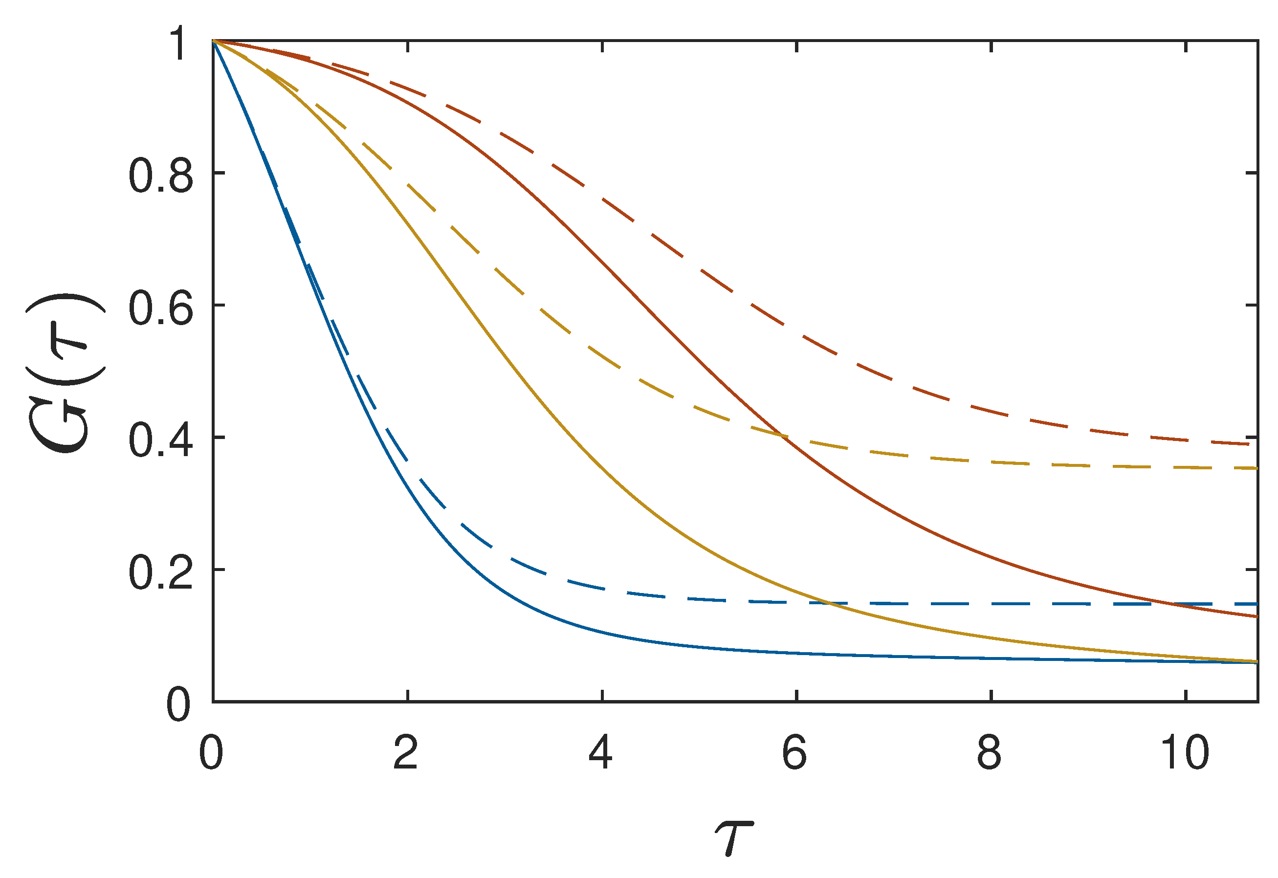
In Figure 3 we compared the resulting fractions

G_{s} (τ)

with the numerically calculated ones for several different choices of the parameters

p_{0}

k_{0}

and

q_{0}

. The agreement is reasonably good for small times but fails at large times. We therefore considered a modified approximate approach valid at all times in Sestion Section 5.3. We first note an important feature of the present solution for vanishing

p_{0} = 0

5.2.2. Comparison with Earlier Results for Vanishing Stellar Evolution $p_{0} = 0$

In the case of vanishing stellar evolution (

p_{0} = 0

) considered before in Section 3 the solution (96) holds for all times. Moreover, in this case the un-approximated full Equation (59) agrees exactly with the approximated Equation (88). Therefore the derived solution (96) had to agree with the solution (32). We checked this consistency noting that for

p_{0} = 0

one has according to Equation (55),

ϵ = 1 + q_{0} - k_{0} = ϵ_{0}

, so that according to Equation (90)

ω = \sqrt{{(1 + q_{0} + k_{0})}^{2} - 4 k_{0}} = \sqrt{χ_{0}^{2} - 4 k_{0}} = ω_{0}

(97)

in terms of the quantities defined in Equation (29) in Section 3. Then Equation (96) reduced to

G (τ) = G_{\infty}^{0} + \frac{ω_{0}}{1 + α_{0} e^{ω τ}},

(98)

with

G_{\infty}^{0} = k_{0} + \frac{ϵ_{0} - ω_{0}}{2} = \frac{χ_{0} - ω_{0}}{2},

(99)

and

α_{0} = \frac{ω_{0} - ϵ_{0} + 2 q_{0}}{ω_{0} + ϵ_{0} - 2 q_{0}} = \frac{ω_{0} + q_{0} + k_{0} - 1}{ω_{0} + 1 - q_{0} - k_{0}} = \frac{ω_{0}}{1 - G_{\infty}^{0}} - 1,

(100)

\begin{matrix} \frac{ω_{0}}{1 - G_{\infty}^{0}} - 1 & = & \frac{ω_{0} - 1 + G_{\infty}^{0}}{1 - G_{\infty}^{0}} = \frac{2 ω_{0} - 1 + χ_{0} - ω_{0}}{2 + ω_{0} - χ_{0}} \\ = & \frac{ω_{0} + q_{0} + k_{0} - 1}{ω_{0} + 1 - q_{0} - k_{0}} . \end{matrix}

(101)

Consequently, Equation (98) agrees exactly with the earlier solution (32). This completes the proof of consistency.

5.3. Modified Approximation for General Times

For non-zero values of

p_{0} > 0

we used the earlier derived Equation (87) based on relation (83) to obtain for the gas fraction

G (τ) = k_{0} + p_{0} + U^{'} (τ) = \frac{1}{1 - c_{1} + c_{1} e^{\frac{τ}{1 - c_{1}}}} .

(102)

We noted before that with the relation (83) the initial and final conditions for

U^{'} (τ)

are fulfilled, as can also be seen from Equation (102) yielding

G (0) = G_{\infty} = 0

. Equation (102) readily provided

G^{'} (τ) = U^{''} (τ) = - \frac{c_{1} e^{\frac{τ}{1 - c_{1}}}}{(1 - c_{1}) {[1 - c_{1} + c_{1} e^{\frac{τ}{1 - c_{1}}}]}^{2}} .

(103)

In order to determine the remaining parameter

c_{1}

we here used the exact condition (48) for

G^{'} (0) = - q_{0}

yielding

\frac{c_{1}}{1 - c_{1}} = q_{0},

(104)

so that

\begin{matrix} c_{1} & = & \frac{q_{0}}{1 + q_{0}}, α_{2} = p_{0} + k_{0} - 1 - q_{0} = - ϵ, \\ α_{1} & = & p_{0} + k_{0}, ϵ = 1 + q_{0} - (p_{0} + k_{0}) \end{matrix}

(105)

We then found for the gas fraction (102)

G (τ) = \frac{1 + q_{0}}{1 + q_{0} e^{(1 + q_{0}) τ}} = \frac{1 + q_{0}}{1 + e^{(1 + q_{0}) (τ - τ_{G})}},

(106)

with

τ_{G} = - \frac{ln q_{0}}{1 + q_{0}} .

(107)

This time scale is solely determined by the ratio

q_{0}

of spontaneous to triggered star formation. Likewise, Equation (69) reads

Y (τ) = \frac{q_{0} e^{α_{1} τ} + e^{- ϵ τ}}{1 + q_{0}},

(108)

providing for the luminous stellar matter fraction (45)

\begin{matrix} \frac{S (τ) + q_{0}}{q_{0}} & = & \frac{1 + (k_{0} + p_{0}) \int_{0}^{τ} d x Y (x)}{Y (τ)} \\ = & \frac{1 + q_{0} e^{α_{1} τ} + \frac{α_{1}}{ϵ} (1 - e^{- ϵ τ})}{q_{0} e^{α_{1} τ} + e^{- ϵ τ}} \\ = & 1 + \frac{(1 + \frac{α_{1}}{ϵ}) (1 - e^{- ϵ τ})}{q_{0} e^{α_{1} τ} + e^{- ϵ τ}}, \end{matrix}

(109)

so that

\begin{matrix} S (τ) & = & \frac{q_{0} (α_{1} + ϵ) [1 - e^{- ϵ τ}]}{ϵ [q_{0} e^{α_{1} τ} + e^{- ϵ τ}]} = \frac{q_{0} (1 + q_{0}) [1 - e^{- ϵ τ}]}{ϵ [q_{0} e^{α_{1} τ} + e^{- ϵ τ}]} \\ = & \frac{q_{0} (1 + q_{0}) [e^{ϵ τ} - 1]}{ϵ [q_{0} e^{(1 + q_{0}) τ} + 1]} = \frac{q_{0} (1 + q_{0}) [e^{ϵ τ} - 1]}{ϵ [1 + e^{(1 + q_{0}) (τ - τ_{G})}]} \\ = & \frac{q_{0} [e^{ϵ τ} - 1]}{ϵ} G (τ), \end{matrix}

(110)

which correctly reproduces

S (0) = S_{\infty} = 0

. The first derivative of the fraction (110) vanishes at the time

τ_{S}

given by the solution of the Eq.

[q_{0} e^{(1 + q_{0}) τ_{S}} + 1] ϵ e^{ϵ τ_{S}} = q_{0} (1 + q_{0}) e^{(1 + q_{0}) τ_{S}} [e^{ϵ τ_{S}} - 1],

(111)

leading to

(p_{0} + k_{0}) e^{(1 + q_{0}) τ_{S}} - (1 + q_{0}) e^{(p_{0} + k_{0}) τ_{S}} = \frac{ϵ}{q_{0}} .

(112)

As the first term dominates the left-hand side of the last Eq. we obtained approximately

τ_{S} ≃ \frac{1}{1 + q_{0}} (- ln (q_{0}) + ln \frac{ϵ}{p_{0} + k_{0}}) = τ_{G} + \frac{ln \frac{ϵ}{p_{0} + k_{0}}}{1 + q_{0}},

(113)

which is slightly larger than the time scale (107). Replacing

τ

in Equation (110) by

τ_{S}

from Equation (113) we found for the peak stellar matter ratio

S_{\max} = S (τ_{S}) ≃ e^{- (p_{0} + k_{0}) τ_{S}} ≃ {[\frac{q_{0} (1 + q_{0})}{1 + q_{0} - p_{0} - k_{0}}]}^{\frac{p_{0} + k_{0}}{1 + q_{0}}} .

(114)

According to Equations (14a) and (17) one has

j (τ) = - \frac{d G (τ)}{d τ} + k_{0} S (τ),

(115)

where

- \frac{d G (τ)}{d τ} = - U^{''} (τ) = \frac{{(1 + q_{0})}^{2}}{4 {cosh}^{2} \frac{(1 + q_{0}) (τ - τ_{G})}{2}} .

(116)

For small values of

k_{0}

, that is

k_{0} ≪ 1

k_{0} S (τ) \leq k_{0} S_{\max} ≃ k_{0} {[\frac{q_{0} (1 + q_{0})}{1 + q_{0} - p_{0} - k_{0}}]}^{\frac{p_{0} + k_{0}}{1 + q_{0}}}

(117)

is negligibly smaller than

| G^{'} (τ) |

, so that the formation rate of new stars (115) reduced to

j (τ) ≃ - G^{'} (τ) = \frac{{(1 + q_{0})}^{2}}{4 {cosh}^{2} \frac{(1 + q_{0}) (τ - τ_{G})}{2}} .

(118)

This formation rate attains its maximum value

j_{\max} = {(\frac{1 + q_{0}}{2})}^{2}

(119)

at the peak time

τ_{j} ≃ τ_{G}

, where

τ_{G}

is was introduced in Equation (107). Most noteworthy, both the maximum value and the peak time are solely determined by the ratio

q_{0}

of the spontaneous to triggered star formation rates, whereas the two other ratios

p_{0}

and

k_{0}

do not enter here.

Finally, the fraction of locked-in matter followed from the sum constraint as

\begin{matrix} L (τ) & = & 1 - G (τ) - S (τ) \\ = & 1 - \frac{1 + q_{0}}{1 + e^{(1 + q_{0}) (τ - τ_{G})}} - \frac{q_{0} (1 + q_{0}) [e^{ϵ τ} - 1]}{ϵ [q_{0} e^{(1 + q_{0}) τ} + 1]} \\ = & 1 - \frac{1 + q_{0}}{1 + e^{(1 + q_{0}) (τ - τ_{G})}} [1 + \frac{q_{0} (e^{ϵ τ} - 1)}{ϵ}], \end{matrix}

(120)

where we inserted Equations (106) and (110). The derived expressions (106), (110), and (120) for

G (τ)

S (τ)

, and

L (τ)

were used in the following sections.

6. Cosmic Star Formation History

As in part I we considered the cosmic star formation history (SFH) of the universe which is proportional to the star formation rate (6). In the following the SFR density and the integrated stellar density using our results from the earlier Section 5.3 are calculated, and compared with data collected by [7].

According to Equations (I-46) and (I-47) as well as Equations (9)–(10) for general

j (τ)

the theoretical cosmic SFR density and the integrated stellar density as a function of redshift are

ψ_{GSL} (z) = A_{1} \frac{j (τ (z))}{{(1 + z)}^{5 / 2}}

(121)

with

A_{1} = 2.78 \cdot 10^{- 10} a_{0}^{2} h_{70} = 2.78 \cdot 10^{- 44} {\tilde{a}}_{0}^{2} h_{70} kg m^{- 3} s,

(122)

and

\begin{matrix} ρ_{GSL}^{*} (z) & = & B_{1} \int_{z}^{1100} d z^{'} [1 - L (z^{'}) - G (z^{'})] \frac{j (τ (z^{'}))}{{(1 + z^{'})}^{5}} \\ = & B_{1} \int_{z}^{1100} d z^{'} S (z^{'}) \frac{j (τ (z^{'}))}{{(1 + z^{'})}^{5}}, \end{matrix}

(123)

with

B_{1} = 2.24 \cdot 10^{8} a_{0}^{2} = 2.24 \cdot 10^{- 26} {\tilde{a}}_{0}^{2} kg m^{- 3} .

(124)

In part I we have argued that the factor

1 - L (z)

enters the calculation of

ρ_{GSL}^{*} (z)

but not the calculation of the SFR density (121) because all stars are born as luminous main sequence stars but only the fraction

1 - L (z)

contributes to the observed integrated density of luminous stars. Here we refined this reduction factor to

1 - L (z) - G (z) = S (z)

as also the baryonic gas does not contribute to the integrated luminous stellar density.

6.1. Observational Constraints

For the comparison with the predictions of the GSL-model we required the same five constraints as in part I.

First, the observed peak SFR density is given by ´

\begin{matrix} ψ (z_{E}) & = & 0 . 178_{- 0.044}^{+ 0.372} M_{⊙} {yr}^{- 1} {Mpc}^{- 3} \\ = & (3 . 83_{- 0.95}^{+ 8.00}) \cdot 10^{- 46} kg s^{- 1} m^{- 3}, \end{matrix}

(125)

and occurs in the redshift range

1.62 - 1.88

([8]) and

1.7 - 2.5

([9]).

Secondly, we required for the observed peak redshift

z_{E} = 2.0 \pm 1.0 .

(126)

As third constraint we used the observed integrated stellar mass density at

z = 0

([10,11])

\begin{matrix} ρ^{*} (0) & = & (5 . 62_{- 1.35}^{+ 1.79}) \cdot 10^{8} \frac{M_{⊙}}{{Mpc}^{3}} \\ = & (3 . 80_{- 0.91}^{+ 1.21}) \cdot 10^{- 29} kg m^{- 3} \end{matrix}

(127)

As fourth constraint we demanded that

{(d ψ / d z)}_{z = 0} > 0

in order to have at least one maximum of

ψ (z)

at positive z. As fifth more stringent constraint we required that

ψ_{GSL} (z)

exhibits exactly one maximum within the redshift range

z \in [0, 8]

6.2. SFR Density

Using Equation (118) for

j (τ)

and Equation (10) for

τ (z)

the SFR density (121) became

\begin{matrix} ψ_{GSL} (τ (z)) & = & \frac{A_{1} {(1 + q_{0})}^{2} Ψ (τ)}{4 ϕ^{5 / 3}}, \end{matrix}

(128a)

\begin{matrix} Ψ (τ) & = & \frac{τ^{5 / 3}}{{cosh}^{2} \frac{(1 + q_{0}) (τ - τ_{G})}{2}} . \end{matrix}

(128b)

This SFR density (128) fulfills the fourth and fifth constraint mentioned in the last Section 6.1. With the first derivative

\begin{matrix} \frac{d Ψ (τ)}{d τ} & = & \frac{5}{3} \frac{τ^{2 / 3}}{{cosh}^{2} \frac{(1 + q_{0}) (τ - τ_{G})}{2}} \times \\ [1 - \frac{3}{5} (1 + q_{0}) τ tanh \frac{(1 + q_{0}) (τ - τ_{G})}{2}] \end{matrix}

(129)

we found that a single maximum occurs at

τ_{E}

given by the solution of the transcendental equation

tanh \frac{(1 + q_{0}) (τ_{E} - τ_{G})}{2} = \frac{5}{3 (1 + q_{0}) τ_{E}},

(130)

while

Ψ_{\max} = τ_{E}^{- 1 / 3} [τ_{E}^{2} - \frac{25}{9 {(1 + q_{0})}^{2}}] .

(131)

Using the following abbreviations,

X = \frac{(1 + q_{0}) τ_{E}}{2}, X_{u} = \frac{(1 + q_{0}) τ_{G}}{2} = - \frac{ln q_{0}}{2},

(132)

Equation (130) simplified to

tanh (X - X_{u}) = \frac{5}{6 X} .

(133)

For values of

0 \leq X_{u} < 3

, corresponding to

e^{- 6} = 2.48 \cdot 10^{- 3} \leq q_{0} \leq 1

, the positive solution of Equation (133) with a maximum relative deviation of 0.9% from the exact solution is given by

\begin{matrix} X (q_{0} \leq 1) & = & \frac{(1 + q_{0}) τ_{E}}{2} ≃ 1.06 (1 + \frac{X_{u}^{1.3}}{2}) \\ ≃ & 1.06 [1 + 0.192 {(- ln q_{0})}^{1.3}], \end{matrix}

(134)

where

X ≃ 1.06

is the numerical solution of

tanh (X) = 5 / (6 X)

. Values

q_{0} \in [0.01, 1]

correspond to values of

X_{u} \in [0, 2.3]

. For values

X_{u} < 0

, corresponding to values of

q_{0} > 1

, the positive solution of Equation (133) with a maximum relative deviation of 0.4% from the exact solution is given by

\begin{matrix} X (q_{0} > 1) & ≃ & \frac{5}{6} + (1.06 - \frac{5}{6}) e^{5 X_{u} / 3} \\ = & \frac{5}{6} [1 + 0.272 e^{5 X_{u} / 3}] = \frac{5}{6} [1 + \frac{0.272}{q_{0}^{5 / 6}}] . \end{matrix}

(135)

This approximation is exact at

X_{u} = 0

and

X_{u} \to - \infty

, and compared with the numerical solution in Figure 4. The cases

q_{0} \leq 1

and

q_{0} > 1

will be discussed in turn.

6.2.1. Values $q_{0} \leq 1$

With Equations (10) and (134) we found for the peak time

τ_{E} (q_{0} \leq 1) = \frac{2.12 [1 + 0.192 {(- ln q_{0})}^{1.3}]}{1 + q_{0}},

(136)

the peak redshift

z_{E} (q_{0} \leq 1) = {(\frac{2.533 {\tilde{a}}_{0} (1 + q_{0})}{h_{70} [1 + 0.192 {(- ln q_{0})}^{1.3}]})}^{2 / 3} - 1

(137)

and the the peak SFR density

\begin{matrix} Ψ_{\max} (q_{0} \leq 1) & = & 3.4986 {(\frac{1 + 0.192 {(- ln q_{0})}^{1.3}]}{1 + q_{0}})}^{5 / 3} \times \\ [1 - \frac{0.618}{{[1 + 0.192 {(- ln q_{0})}^{1.3}]}^{2}}], \end{matrix}

(138)

so that

ψ_{GSL} (z_{E}, q_{0} \leq 1) = 4.2205 \cdot 10^{- 46} {\tilde{a}}_{0}^{1 / 3} h_{70}^{8 / 3} {(1 + q_{0})}^{2} Ψ_{\max}

= 1.477 \cdot 10^{- 45} {\tilde{a}}_{0}^{1 / 3} h_{70}^{8 / 3} {(1 + q_{0})}^{1 / 3} {(1 + 0.067 {(- ln q_{0})}^{3 / 2})}^{5 / 3} \times

[1 - \frac{0.618}{{[1 + 0.192 {(- ln q_{0})}^{1.3}]}^{2}}] kg s^{- 1} m^{- 3},

(139)

Equating Equation (137) with the observed peak redshift (126) readily yielded

{\tilde{a}}_{0} (q_{0} \leq 1) = (2 . 05_{- 0.93}^{+ 1.11}) \frac{h_{70} [1 + 0.192 {(- ln q_{0})}^{1.3}]}{1 + q_{0}},

(140)

while the equality of Equation (139) with the observed peak SFR density (125) lead to

{\tilde{a}}_{0} (q_{0} \leq 1) = \frac{(0 . 0174_{- 0.010}^{+ 0.496}) h_{70}^{- 8} {(1 + q_{0})}^{- 1}}{{[1 + 0.192 {(- ln q_{0})}^{1.3}]}^{5} {[1 - \frac{0.618}{{[1 + 0.192 {(- ln q_{0})}^{1.3}]}^{2}}]}^{3}} .

(141)

Note that for

q_{0} = 1

Equations (140) and (141) provide (Figure 5)

\begin{matrix} {\tilde{a}}_{0} (q_{0} = 1) & = & (1 . 03_{- 0.47}^{+ 0.56}) h_{70}, \end{matrix}

(142a)

\begin{matrix} {\tilde{a}}_{0} (q_{0} = 1) & = & (0 . 156_{- 0.089}^{+ 4.449}) h_{70}^{- 8}, \end{matrix}

(142b)

which overlap very well.

6.2.2. Values $q_{0} > 1$

With Equations (10) and (135) we obtained for the peak time

τ_{E} (q_{0} > 1) = \frac{5}{3} \frac{0.272 + q_{0}^{5 / 6}}{q_{0}^{5 / 6} (1 + q_{0})},

(143)

the peak redshift

z_{E} (q_{0} > 1) = {(\frac{3.222 {\tilde{a}}_{0} q_{0}^{5 / 6} (1 + q_{0})}{h_{70} [0.272 + q_{0}^{5 / 6}]})}^{2 / 3}, - 1

(144)

and the peak SFR density

\begin{matrix} Ψ_{\max} (q_{0} > 1) = 2.343 [1 - \frac{q_{0}^{5 / 3}}{{(0.272 + q_{0}^{5 / 6})}^{2}}] {(\frac{0.272 + q_{0}^{5 / 6}}{q_{0}^{5 / 6} (1 + q_{0})})}^{5 / 3}, \end{matrix}

(145)

so that

ψ_{GSL} (z_{E}, q_{0} > 1)

= 4.2205 \cdot 10^{- 46} {\tilde{a}}_{0}^{1 / 3} h_{70}^{8 / 3} {(1 + q_{0})}^{2} Ψ_{\max}

= 9.889 \cdot 10^{- 46} {\tilde{a}}_{0}^{1 / 3} h_{70}^{8 / 3} {(1 + q_{0})}^{2} {(\frac{0.272 + q_{0}^{5 / 6}}{q_{0}^{5 / 6} (1 + q_{0})})}^{5 / 3} \times

[1 - \frac{q_{0}^{5 / 3}}{{(0.272 + q_{0}^{5 / 6})}^{2}}] kg s^{- 1} m^{- 3} .

(146)

Equating Equation (144) with the observed peak redshift (126) readily yielded

{\tilde{a}}_{0} (q_{0} > 1) = (1 . 61_{- 0.74}^{+ 0.87}) \frac{h_{70} [0.272 + q_{0}^{5 / 6}]}{q_{0}^{5 / 6} (1 + q_{0})},

(147)

while the equality of Equation (146) with the observed peak SFR density (125) lead to

\begin{matrix} {\tilde{a}}_{0} (q_{0} > 1) & = & \frac{(0 . 0581_{- 0.0334}^{+ 1.653})}{h_{70}^{8} (1 + q_{0})} {[\frac{q_{0}^{5 / 6}}{0.272 + q_{0}^{5 / 6}}]}^{5} \times \\ {[1 - \frac{q_{0}^{5 / 3}}{{(0.272 + q_{0}^{5 / 6})}^{2}}]}^{- 3} . \end{matrix}

(148)

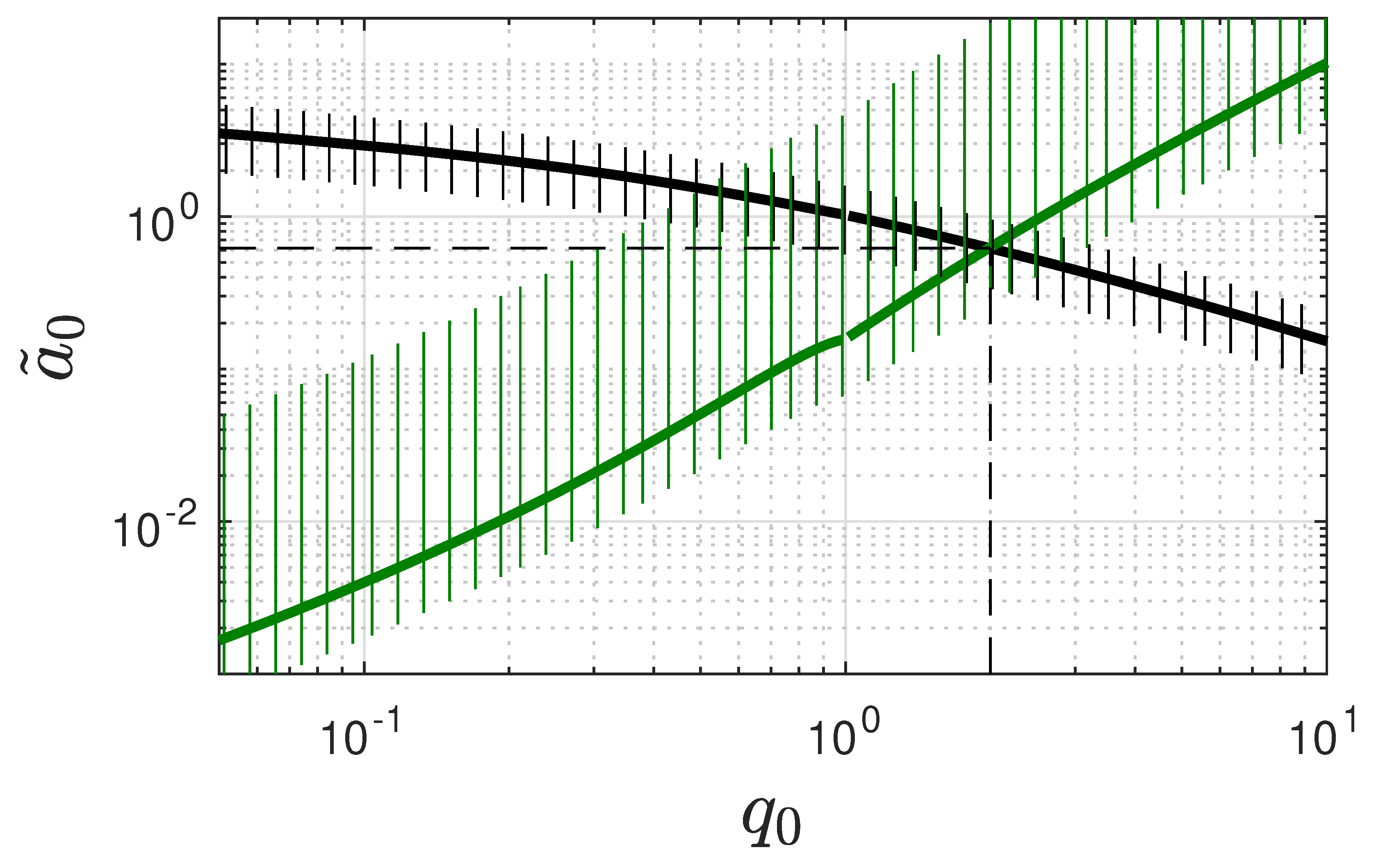
All four expressions (140)–(141) and (147)–(148) for

{\tilde{a}}_{0}

are displayed in Figure 5. As parameter values consistent with the observational constraints values we inferred from Figure 5

\begin{matrix} {\tilde{a}}_{0} & = & 0 . 62_{- 0.29}^{+ 0.33}, q_{0} = 2 . 0_{- 1.1}^{+ 1.2}, \end{matrix}

(149)

implying

\begin{matrix} a_{0} & = & (0 . 62_{- 0.29}^{+ 0.33}) \cdot 10^{- 17} Hz, \end{matrix}

(150a)

\begin{matrix} β_{0} & = & a_{0} q_{0} = (1 . 24_{- 0.94}^{+ 1.80}) \cdot 10^{- 17} Hz . \end{matrix}

(150b)

Consequently, the spontaneous and triggered star formation processes operate on time scales of

t_{spont} ≃ 2 . 57_{- 1.52}^{+ 8.15}

Gyr and

t_{trig} ≃ 5 . 13_{- 1.78}^{+ 4.52}

Gyr, respectively. The partly large error bars resulted from the large error bars on the observed SFR peak density (125).

Note that for

q_{0} = 1

the Equations (147) and (148) provide

\begin{matrix} {\tilde{a}}_{0} (q_{0} = 1) & = & (1 . 02_{- 0.47}^{+ 0.55}) h_{70}, \end{matrix}

(151a)

\begin{matrix} {\tilde{a}}_{0} (q_{0} = 1) & = & (0 . 157_{- 0.090}^{+ 4.455}) h_{70}^{- 8}, \end{matrix}

(151b)

which agree perfectly with the earlier estimate (142). For very large values of

q_{0} ≫ 1

Equations (147) and (148) yielded

\begin{matrix} {\tilde{a}}_{0} (q_{0} ≫ 1) & = & (1 . 61_{- 0.74}^{+ 0.87}) \frac{h_{70}}{q_{0}}, \end{matrix}

(152a)

\begin{matrix} {\tilde{a}}_{0} (q_{0} ≫ 1) & = & (0 . 0581_{- 0.0334}^{+ 1.653}) \cdot 6.21 q_{0}^{3 / 2} h_{70}^{- 8} . \end{matrix}

(152b)

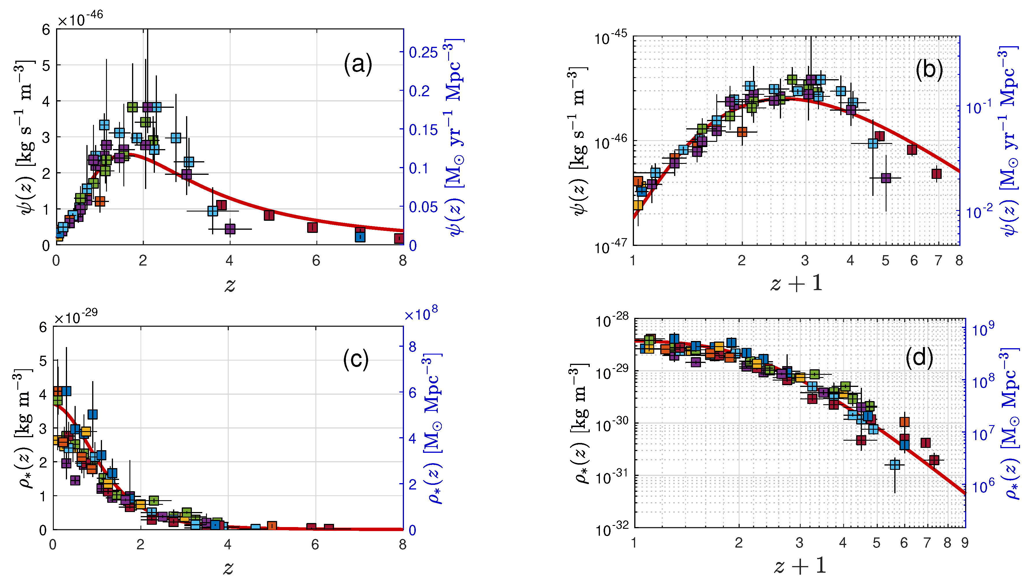
In panels (a) and (c) of Figure 6 we compared the theoretical SFR density (128) with the observations collected by [7] where we varied freely the parameters

{\tilde{a}}_{0}

and

q_{0}

. As can be seen we obtained excellent agreement with the observations for the parameter choice

{\tilde{a}}_{0} = 0.368

and

q_{0} = 2.67

. Both values are consistent with the range of parameter values (149) implied by the observational constraints discussed before. In panels (b) and (d) we show the corresponding fit to the observations of the integrated stellar density, to be discussed next. Here again we found excellent agreement if additionally the parameter values

k_{0} = 0.0039

and

p_{0} = 0.656

so that

k_{0} + p_{0} = 0.66

was chosen.

6.3. Integrated Stellar Density

Likewise, the integrated stellar density (123) is given by

ρ_{GSL}^{*} (z) = \frac{2 B_{1}}{3 ϕ^{8 / 3}} \int_{\frac{ϕ}{1101^{3 / 2}}}^{\frac{ϕ}{{(1 + z)}^{3 / 2}}} d τ j (τ) S (τ) τ^{5 / 3}

≃ \frac{B_{1} q_{0} {(1 + q_{0})}^{3}}{6 ϵ ϕ^{8 / 3}} \int_{0}^{\frac{ϕ}{{(1 + z)}^{3 / 2}}} d τ \frac{τ^{5 / 3}}{{cosh}^{2} \frac{(1 + q_{0}) (τ - τ_{G})}{2}} \frac{e^{ϵ τ} - 1}{1 + e^{(1 + q_{0}) (τ - τ_{G})}}

= \frac{B_{1} q_{0} {(1 + q_{0})}^{3}}{12 ϵ ϕ^{8 / 3}} \int_{0}^{\frac{ϕ}{{(1 + z)}^{3 / 2}}} d τ \frac{τ^{5 / 3} e^{- \frac{(1 + q_{0}) (τ - τ_{G})}{2}}}{{cosh}^{3} \frac{(1 + q_{0}) (τ - τ_{G})}{2}} (e^{ϵ τ} - 1)

= \frac{2^{2 / 3} B_{1} q_{0}^{1 / 2} {(1 + q_{0})}^{1 / 3}}{3 ϵ ϕ^{8 / 3}} J (\frac{(1 + q_{0}) ϕ}{2 {(1 + z)}^{3 / 2}}),

(153)

where we used Equations (10), (110) and (118), substituted according to Equation (132), and introduced the integral

\begin{matrix} J (A) & = & \int_{0}^{A} d X \frac{X^{5 / 3} e^{- X} [e^{\frac{2 ϵ X}{1 + q_{0}}} - 1]}{{cosh}^{3} (X - X_{u})} . \end{matrix}

(154)

6.3.1. Asymptotics of the Integral (154)

We investigated the asymptotic behavior of the integral (154) for small values of A with respect to unity, corresponding to large values of the redshift z. We obtained

\begin{matrix} J (A ≪ 1) & ≃ & \frac{2 ϵ}{1 + q_{0}} \int_{0}^{A} d X \frac{X^{8 / 3}}{{cosh}^{3} (X - X_{u})} \\ ≃ & \frac{6 ϵ A^{11 / 3}}{11 (1 + q_{0}) {cosh}^{3} (X_{u})} = \frac{48 ϵ q_{0}^{3 / 2} A^{11 / 3}}{11 {(1 + q_{0})}^{4}} . \end{matrix}

(155)

A (z) = (1 + q_{0}) ϕ / (2 {(1 + z)}^{3 / 2})

the asymptotics (155) corresponds to

J (z \geq z_{c}) ≃ \frac{3 \cdot 2^{1 / 3} ϵ q_{0}^{3 / 2} ϕ^{11 / 3}}{11 {(1 + q_{0})}^{1 / 3} {(1 + z)}^{11 / 2}},

(156)

with the characteristic redshift

z_{c} = {[\frac{1 + q_{0}) ϕ}{2}]}^{2 / 3} - 1 = 1.93 {[\frac{(1 + q_{0}) {\tilde{a}}_{0}}{h_{70}}]}^{2 / 3} - 1

(157)

of order unity. We then obtained for Equation (153) in this limit

\begin{matrix} ρ_{GSL}^{*} (z \geq z_{c}) & ≃ & \frac{2 B_{1} q_{0}^{2} ϕ}{11 {(1 + z)}^{11 / 2}} \\ = & \frac{2.19 \cdot 10^{- 26} q_{0}^{2} {\tilde{a}}_{0}^{3}}{h_{70} {(1 + z)}^{11 / 2}} kg m^{- 3} . \end{matrix}

(158)

This asymptotic is significantly steeper than the

{(1 + z)}^{- 4}

behavior obtained in part I for neglected triggered star formation.

In the alternative case of large arguments

A ≫ 1

the integral (154) was approximated in Appendix B as

\begin{matrix} J (A ≫ 1) & ≃ & \frac{3}{2 {cosh}^{3} (X_{u})} [{(\frac{4}{3} + \frac{2 (k_{0} + p_{0})}{1 + q_{0}})}^{- 8 / 3} - 0.04] \\ = & \frac{12 q_{0}^{3 / 2}}{{(1 + q_{0})}^{3}} [{(\frac{4}{3} + \frac{2 (k_{0} + p_{0})}{1 + q_{0}})}^{- 8 / 3} - 0.04] . \end{matrix}

(159)

6.3.2. Present-Day Integrated Stellar Density

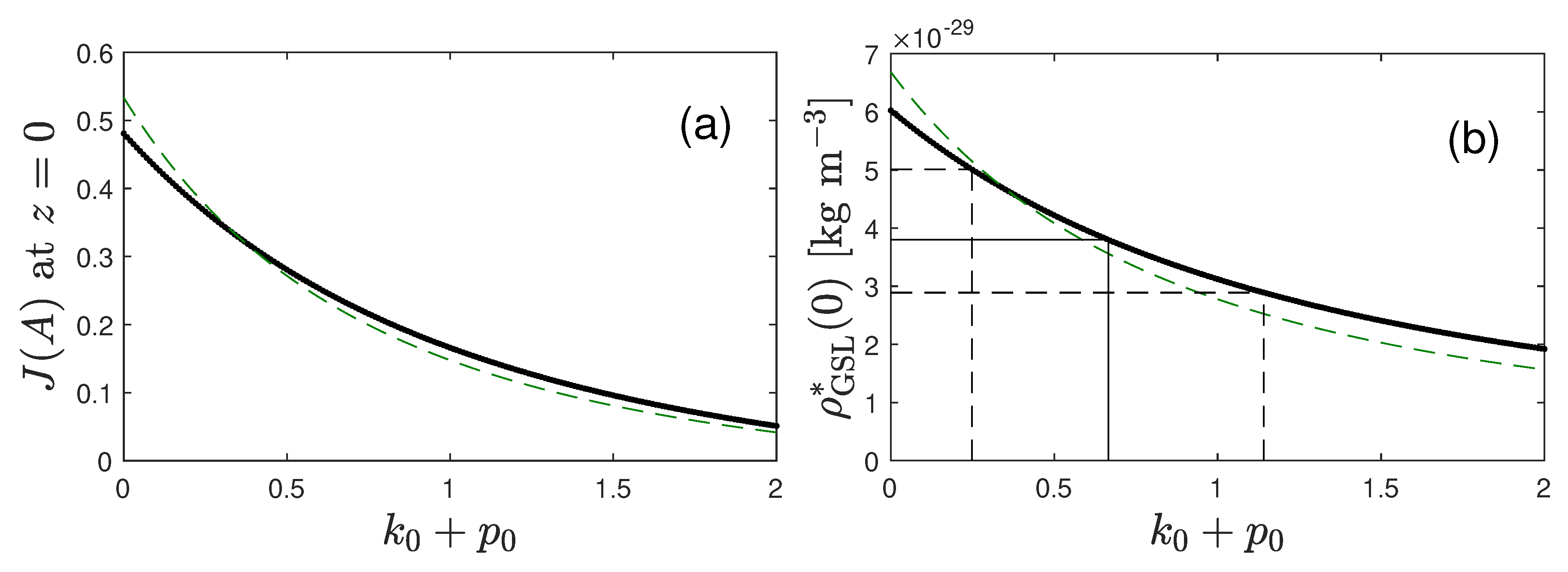
For the present-day integrated stellar density at redshift

z = 0

we note that with our earlier parameter estimates (149)

A (z = 0) = 2.69 (1 + q_{0}) {\tilde{a}}_{0} h_{70}^{- 1} ≃ 4.99

is large compared to unity so that we used the approximation (159) providing for Equation (153)

ρ_{GSL}^{*} (0) ≃ \frac{2^{8 / 3} B_{1} q_{0}^{2}}{ϵ {(1 + q_{0})}^{8 / 3} ϕ^{8 / 3}} [{(\frac{4}{3} + \frac{2 (k_{0} + p_{0})}{1 + q_{0}})}^{- 8 / 3} - 0.04]

= \frac{1.61 \cdot 10^{- 27} h_{70}^{8 / 3} q_{0}^{2}}{{\tilde{a}}_{0}^{2 / 3} ϵ {(1 + q_{0})}^{8 / 3}} [{(\frac{4}{3} + \frac{2 (k_{0} + p_{0})}{1 + q_{0}})}^{- 8 / 3} - 0.04] kg m^{- 3} .

(160)

Equating the constraint (127) with Equation (160) then yielded

{\tilde{a}}_{0} = \frac{(276_{- 94}^{+ 140}) h_{70}^{4} q_{0}^{3}}{{(1 + q_{0} - p_{0} - k_{0})}^{3 / 2} {(1 + q_{0})}^{4}} {[{(\frac{4}{3} + \frac{2 (k_{0} + p_{0})}{1 + q_{0}})}^{- 8 / 3} - 0.04]}^{3 / 2} .

(161)

In contrast with the earlier constraints (140) and (141) the constraint (161) depends on the sum

p_{0} + k_{0}

of the additional ratios

k_{0}

and

p_{0}

characterizing the strength of stellar evolution and feedback, respectively. For

{\tilde{a}}_{0}

and

q_{0}

from Equation (149), Equation (161) yielded

k_{0} + p_{0} = 0 . 585_{- 0.317}^{+ 0.574}

in excellent agreement with the numerical fit in Figure 7.

7. Redshift Dependency of the Gas and Stellar Fractions and Future of the Baryonic Universe

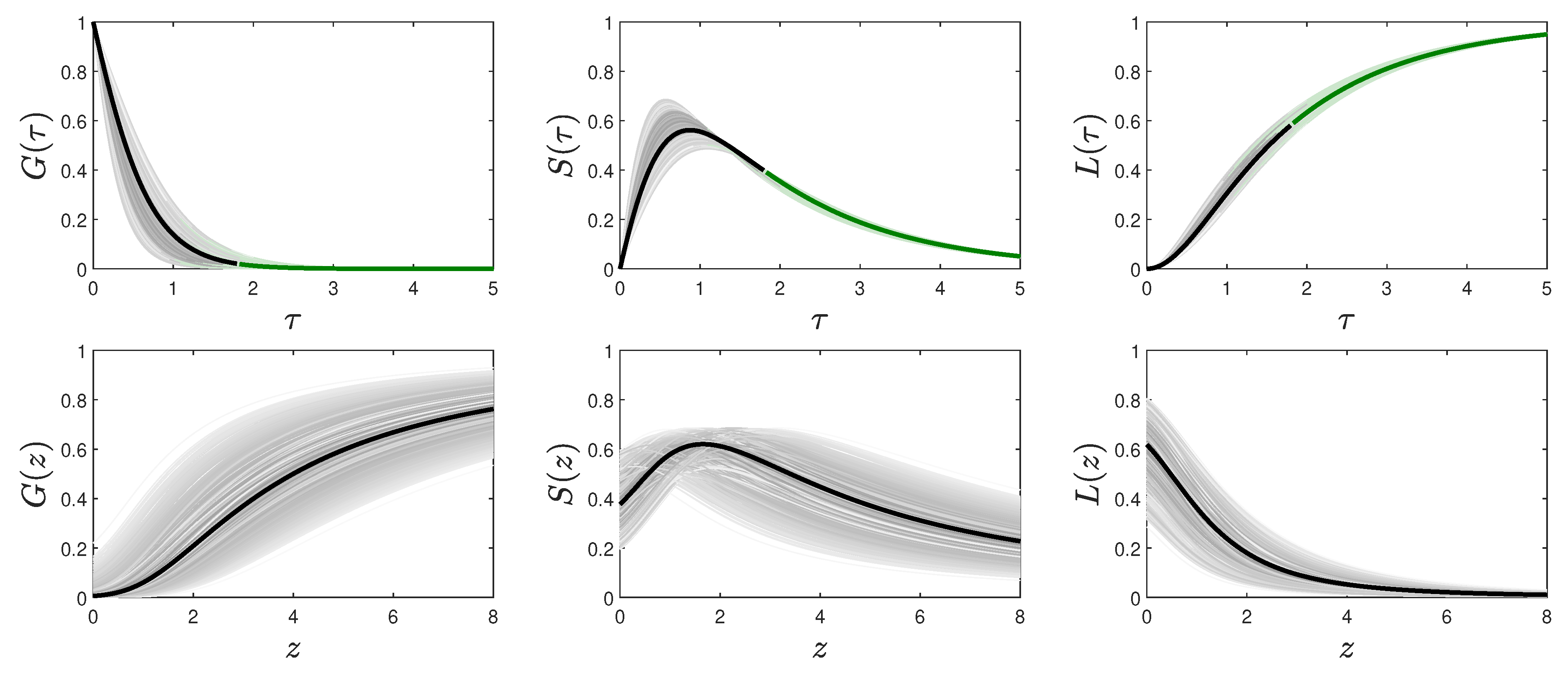
Here the best fit parameter values for the three ratios

q_{0}

p_{0}

and

k_{0}

and the triggered star formation rate

a_{0}

from the last Section were used to determine the present-day (

z = 0

) gas and stellar fractions. The three panels in Figure 8 display the resulting reduced time and redshift dependencies of the fractions using Equations (106), (110), and (120). The error bars according to Equations (149) and

k_{0} + p_{0} \in [0.25, 1.14]

from the fits in Figure 7 are represented as gray lines, whose darkness moderately increases with their probability, assuming Gaussian distributed

{\tilde{a}}_{0}

and

q_{0}

These panels not only show the history of the cosmological gas and stellar fractions as a function of redshift z in panel (b), but also their future evolution as a function of the reduced time

τ

in panel (a). Note that the present-day epoch depending on

{\tilde{a}}_{0}

corresponds to about

τ (z = 0) = 1.83

, so that future starts beyond this time. In panel (a) of Figure 8 we marked the future epochs in green colour. It is clear, however, that ultimately at

τ = \infty

the stationary state with values

G_{\infty} = 0, \frac{G_{\infty}}{1 - G_{\infty}} = 0, \frac{G_{\infty}}{S_{\infty}} = 0

(162)

is attained.

Next we considered the present-day (

z = 0

) gas and stellar fractions. As present-day quantities have to be calculated, we used the modification

ζ (0)

in Equations (10)–(12) for

τ (z = 0))

7.1. Present-Day Gas Fraction

According to Equation (106) the Equation (10) predicts for the present-day gas fraction

\begin{matrix} G (z = 0) & = & \frac{1 + q_{0}}{1 + q_{0} e^{(1 + q_{0}) τ (0)}} = \frac{1 + q_{0}}{1 + q_{0} e^{2.94 (1 + q_{0}) {\tilde{a}}_{0} h_{70}^{- 1}}}, \end{matrix}

(163)

which can be contrasted with the observed Milky Way gas fraction of

\approx 0.1

([12]). With the parameters (149) we obtained for

h_{70} = 1

G (z = 0) = 0 . 00631_{- 0.00629}^{+ 0.278}

(164)

Within the large error bars this prediction is consistent with the observed gas fraction of about 10 percent.

The gas fraction (164) also provided the present-day interstellar gas mass to total (including locked-in matter) stellar mass

\begin{matrix} \frac{G (z = 0)}{S (z = 0) + L (z = 0)} & = & \frac{G (z = 0)}{1 - G (z = 0)} = 0.00635 \end{matrix}

(165)

for the nominal parameter values

q_{0} = 2

and

{\tilde{a}}_{0} = 0.62

7.2. Stellar Fractions

Likewise, from Equation (110) we obtained

\begin{matrix} S (z = 0) & = & \frac{q_{0} [e^{ϵ τ (0)} - 1] G (z = 0)}{ϵ} \\ = & \frac{q_{0} [e^{2.94 ϵ {\tilde{a}}_{0} h_{70}^{- 1}} - 1] G (z = 0)}{ϵ} . \end{matrix}

(166)

For the nominal values

q_{0} = 2

{\tilde{a}}_{0} = 0.62

p_{0} + k_{0} = 0.66

, so that

ϵ = 2.34

, we found

S (z = 0) = 0 . 379_{- 0.191}^{+ 0.224}, L (z = 0) = 0 . 615_{- 0.378}^{+ 0.197}

(167)

for the ratio of the present-day interstellar gas mass to luminous stellar mass

\begin{matrix} \frac{G (z = 0)}{S (z = 0)} & = & 0 . 01665_{- 0.01665}^{+ 0.5627} . \end{matrix}

(168)

The last ratio could be compared with the observed gas/stellar mass fraction in

z \sim 0

galaxies ([13,14]) as the stellar component has been obtained from large galaxy surveys in the optical/infrared band where locked-in stellar matter contributes negligibly small emission. The observations reveal ratios as a function of stellar mass in the range

[0.01, 0.7]

. The estimate (168) is consistent with the observations but excluded the large positive error bar.

The estimates (167) indicated that at the present time the majority of the baryons (more than 72 percent) resides in the form of stellar matter with

61 . 5_{- 37.8}^{+ 19.7}

percent in locked-in stellar matter (white dwarfs, neutron stars and black holes) and

37 . 9_{. 19.1}^{+ 22.4}

percent in the form of luminous main-sequence stars. These estimates had to be contrasted with expectations from stellar evolution models. In these models, for a reasonable choice of the initial mass function (see for example [15,16]), a stellar population of approximately 13 Gyr has only returned about

R \sim

40% of its originally formed mass to the ISM, with

(1 - R) \sim

60% remaining as surviving stars or remnants. Of that ∼ 60%, only around ∼ 25% consists of remnants (white dwarfs, black holes, and neutron stars) — see section 2.1.2 of the review by [17]. Within their uncertainties the estimates (167) are consistent with the stellar evolution model calculations which have their own uncertainties.

7.3. Remarks

We can conclude this Section with two important remarks:

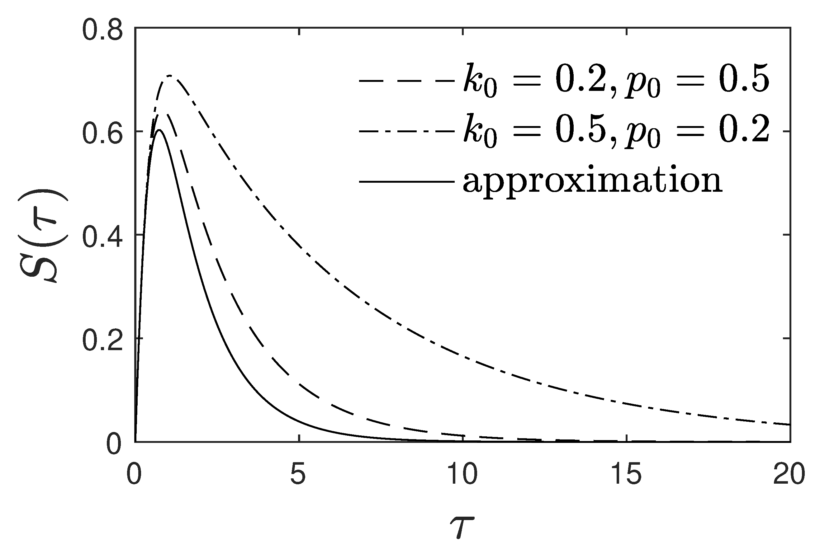
(1) It had not escaped from our attention that we can only constraint analytically the sum of the two parameters

p_{0} + k_{0}

from the comparison of the integrated stellar light as well as the stellar fractions. This is a drawback of our approximation of the exact Equation (73): without the function

R (τ)

this equation indeed only involves the sum

p_{0} + k_{0}

. Therefore any dependence on the individual values of

p_{0}

and

k_{0}

only stems from the function

R (τ)

calculated in Equation (81). However, with the adopted relation (83) involving only

R (\infty)

, which with the choice (84) then also depends only on the sum

p_{0} + k_{0}

, any dependency on the individual values of

p_{0}

und

k_{0}

was not possible anymore. This could be proven by comparing the exact numerical solutions of

S (τ)

for the two cases

(k_{0} = 0.2, p_{0} = 0.5)

and

(k_{0} = 0.5, p_{0} = 0.2

) shown in Figure 9. As in both cases the sum

p_{0} + k_{0} = 0.7

is the same our approximation yielded the same time dependence of

S (τ)

, whereas the exact numerically calculated variations were different.

(2) The second remark concerns the value of the Hubble constant. In contrast to part I we here were in accord with all observational constraints for the standard value

h_{70} = 1

of the Hubble constant and did not have to speculate on substantially smaller values of the Hubble constant as in part I.

8. Summary and Conclusions

In this work we extended the analysis of the compartmental description of the temporal evolution of the baryonic matter in stars and interstellar gas, pioneered in part I, by the inclusion of the triggered star formation process. As in part I the introduction of gaseous and stellar fractions of the total baryonic matter as the basic dynamical variables is advantageous because it allows to apply the analysis to a variety of astrophysical systems. The competition of triggered and spontaneous star formation, stellar feedback and stellar evolution is theoretically investigated with analytical and numerical solutions of the nonlinear dynamical GSL equations for the interstellar and intergalactic gas fraction

G (t)

, the luminous stellar matter fraction

S (t)

, and the locked-in matter fraction

L (t)

By introducing the dimensionless reduced time variable

τ

(8) for arbitrarily but given time-dependent triggered SFR coefficient

a (t)

, as well as the dimensionless ratios

q (t) = β (t) / a (t)

k (t) = b (t) / a (t)

and

p (t) = c (t) / a (t)

, the derived exact solutions of the GSL equations for stationary ratios

q_{0}

k_{0}

and

p_{0}

hold for stationary rates as well as for the case of the same time-dependency of all rates. The accuracy of the analytical solutions is confirmed by comparison with the exact numerical solutions of the GSL equations. Once again of particular interest is the understanding of the cosmic star formation history, the present-day gas and stellar fraction, and their ultimate future fate with compartmental models. For a flat

Λ

CDM Friedmann cosmology the relationship between the reduced time variable

τ (z)

and the cosmological redshift z is used to calculate the effect of redshift on the cosmological star formation rate, the integrated stellar density, and the present-day gas and stellar fractions. In contrast to part I the cosmological star formation rate now has two contributions from the spontaneous and triggered formation processes.

The inclusion of the nonlinear triggered star formation process enormously complicated the derivation of analytical solutions. Exact solutions of the GSL equations were derived in Section 3 for the case of negligible stellar evolution and served an important dual purpose, namely to test the accuracy of the numerical code solving the GSL equations as well as comparing with the analytical approximations derived in the most general case in the respective limit of negligible stellar evolution. For the most general case of all four competing processes operating simultaneously with stationary ratios, we reduced the coupled dynamical GSL equations in Section 3 to one exact nonlinear differential equation (see Equations (59) and (73)) determining the time evolution for

U (τ) = \int_{0}^{τ} d τ^{'} G (τ^{'}) - (p_{0} + k_{0}) τ

from which the gas and stellar fractions can be determined. Approximate analytical solutions were derived in Section 5 for the case of small times

τ \leq p_{0}^{- 1}

and for general times for positive values of the ratio

p_{0}

characterizing the stellar evolution process. The small times solution in the case of negligible stellar evolution (

p_{0} = 0

) holds at all times and agrees exactly with the earlier derived exact solutions in this special case in Section 5. The accuracy of the approximate solution in the general case of finite

p_{0}

is demonstrated by comparison with the numerical solutions. Most noteworthy, for small enough rates of stellar feedback determining the ratio

k_{0}

the derived gas fraction and the formation rate (118) of new stars as a function of the reduced time

τ

are solely determined by the ratio

q_{0}

of spontaneous to triggered star formation, whereas the remaining two ratios

k_{0}

and

p_{0}

exhibit themselves in the temporal evolution of the stellar fractions

S (τ)

and

L (τ)

. This is in accord with the starting reduced GSL equations Equations (14a) and (17) that do not directly involve the ratio

p_{0}

The near independency of the formation rate (118) of new stars as a function of the reduced time

τ

significantly facilitates the calculation of the cosmological SFR as a function of redshift (Section 6) which, for an adopted constant triggered star formation rate

a_{0}

, depends only on the two parameters

a_{0}

and

q_{0} = β_{0} / a_{0}

. The comparison with the observed SFR provides as best fit values

a_{0} = 0.368

and

q_{0} = 2.97

k_{0} = 0.0039

and

p_{0} = 0.656

so that

p_{0} + k_{0} = 0.66

. Due to the partly large uncertainties in the observed peak SFR rate the error bars on these parameters are

{\tilde{a}}_{0} = 0 . 62_{- 0.29}^{+ 0.39}

q_{0} = 2 . 0_{- 1.1}^{+ 1.2}

and

k_{0} + p_{0} = 0 . 585_{- 0.317}^{+ 0.574}

. In Section 7 we calculated the resulting reduced and redshift dependencies of the three gas and stellar fractions. These not only show the history of the cosmological gas and stellar fractions as a function of redshift z, but also predict their future evolution as a function of the reduced time

τ

. Within the error bars the calculated present day gas and stellar fractions are consistent with the observed Milky Way gas fraction of 0.1 as well as the observed gas/stellar mass fraction in

z \sim 0

galaxies. They also agree reasonably well with expectations from stellar evolution models.

As most important result of this investigation we found that the inclusion of the triggered star formation process explains the observed cosmological star formation rate and the integrated stellar density as well as the present-day gas and stellar fractions much better than the simplified GSL-model of part I ignoring triggered star formation. The best fit parameter values to the observations indicate that the spontaneous and triggered star formation processes dominate the dynamical evolution of baryonic matter in the universe indicated by the best-fit value of the sum of ratios

p_{0} + k_{0}

being significantly smaller than unity. For an adopted constant triggered star formation rate

a_{0}

, the spontaneous and triggered star formation processes operate on time scales of

t_{spont} ≃ 2 . 57_{- 1.52}^{+ 8.15}

Gyr and

t_{trig} ≃ 5 . 13_{- 1.78}^{+ 4.52}

Gyr, respectively. Interestingly, the spontaneous formation process is about twice more effective than the triggered formation process.

After the non-perfect agreement of the simplified GSL-model with only spontaneous star formation process investigated in part I, we can now conclude that the inclusion of the triggered star formation process has improved the situation significantly. This generalized GSL-model is consistent with all observational constraints from the cosmological star formation history and the corresponding integrated stellar density. The model provides excellent fits to the observed redshift dependencies of the star formation rate and the integrated stellar density. Moreover, it explains the observed present-day gas and stellar fractions in the universe, and it makes predictions on the future evolution of these fractions in the universe. The presented analysis of the GSL compartmental model has lead to new and original insights on the cosmological baryonic matter cycle in the universe.

Acknowledgments

R.S. gratefully acknowledges the institutional support by the Astrophysics Group headed by Prof. Dr. Wolfgang Duschl and Prof. Dr. Sebastian Wolf at the Institut für Theoretische Physik und Astrophysik of the Christian-Albrechts-Universität in Kiel, Germany.

Appendix A. Reduced Time Redshift Relation

With Equation (9) we obtained for the relation between the reduced time

τ

and the redshift z in a flat

Λ

CDM Friedmann cosmology

\begin{matrix} τ (z) & = & \frac{2 a_{0} [0.424 + f (τ)]}{3 \sqrt{1 - Ω_{0}} H_{0}} = \frac{3.513 {\tilde{a}}_{0} [0.424 + f (τ)]}{h_{70}} s \end{matrix}

(A1)

with

\begin{matrix} f (τ) & = & ln \frac{1 + \sqrt{1 + \frac{Ω_{0}}{1 - Ω_{0}} {(1 + z)}^{3}}}{{(1 + z)}^{\frac{3}{2}}} \\ = & ln \frac{1 + \sqrt{1 + \frac{3}{7} {(1 + z)}^{3}}}{{(1 + z)}^{\frac{3}{2}}}, \end{matrix}

(A2)

where

Ω_{m} = Ω_{0} = 0.3

and

H_{0} = 70 h_{70}

km s⁻¹

{Mpc}^{- 1} = 2.268 \cdot 10^{- 18} h_{70}

s⁻¹ according to Eq. (I-39) for a constant triggered star formation rate

a (t) = a_{0} = 10^{- 17} {\tilde{a}}_{0}

. Equations (A1)–(A2) imply

\begin{matrix} \frac{d f (τ)}{d τ} & = & - \frac{3}{2 (1 + z) \sqrt{1 + \frac{Ω_{0}}{1 - Ω_{0}} {(1 + z)}^{3}}}, \end{matrix}

(A3)

and thus

\begin{matrix} \frac{d τ}{d z} & = & - \frac{a_{0}}{H_{0} \sqrt{Ω_{0}} \sqrt{{(1 + z)}^{3} + \frac{1 - Ω_{0}}{Ω_{0}}}} . \end{matrix}

(A4)

For redshift values

z > {(\frac{1 - Ω_{0}}{Ω_{0}})}^{1 / 3} - 1 = 0.326

(A5)

we approximated, following part I, the Equation (A4) as

\begin{matrix} \frac{d τ}{d z} & ≃ & - \frac{a_{0}}{\sqrt{Ω_{0}} H_{0} {(1 + z)}^{5 / 2}}, \end{matrix}

(A6)

corresponding to

\begin{matrix} τ (z) & ≃ & a_{0} τ_{f} {(1 + z)}^{- 3 / 2}, \end{matrix}

(A7)

\begin{matrix} τ_{f} & = & \frac{2}{3 H_{0} \sqrt{Ω_{0}}} = \frac{5.37 \cdot 10^{17}}{h_{70}} s . \end{matrix}

(A8)

Obviously, the approximations (A6)–(A8) are excellent for redshift values significantly greater than 0.326, but not accurate enough for redshift values close to zero. Here we used the improved approximation

τ_{f} = \frac{2 ζ}{3 H_{0} \sqrt{Ω_{0}}} = 2.94 \cdot 10^{17} h_{70}^{- 1} s,

(A9)

where the factor

ζ = \sqrt{3 / 10} = 0.548

(A10)

ensured that

d τ / d z

is captured exactly at

z = 0

. Note that the exact value from Equation (A4) is

{d τ / d z |}_{z = 0} = - a_{0} / H_{0} \sqrt{10 Ω_{0} / 3}

, where the value from the approximation (A6) is given by

- a_{0} / H_{0} \sqrt{Ω_{0}}

Accordingly, the reduced time redshift relation (A1) for all values of z is well approximated by Equations (10)–(12), that is

\begin{matrix} τ (z) & ≃ & \frac{ϕ}{{(1 + z)}^{3 / 2}}, ϕ = \frac{5.37 {\tilde{a}}_{0} ζ (z)}{h_{70}}, \end{matrix}

(A11)

\begin{matrix} ζ (z) & = & \frac{{(1 + z)}^{3 / 2}}{\sqrt{\frac{7}{3} + {(1 + z)}^{3}}}, \end{matrix}

(A12)

\begin{matrix} ζ (0) & = & \sqrt{\frac{3}{10}} = 0.548 . \end{matrix}

(A13)

Appendix B. Present-Day Integrated Stellar Density

In Equation (154) we introduced this integral

\begin{matrix} J (A) & = & \int_{0}^{A} \frac{X^{5 / 3} e^{- X} [e^{2 c X} - 1] d X}{{cosh}^{3} (X - X_{u})}, c = 1 - \frac{k_{0} + p_{0}}{1 + q_{0}} . \end{matrix}

(A14)

We were interested in an approximation to this integral in the vicinity of

q_{0} \approx 2

and

A \approx 5

. The integrand basically vanishes for

X \geq 5

for any

k_{0} + p_{0} \in [0, 1]

, so that

J (A) ≃ J (\infty) = \int_{0}^{\infty} d X \frac{X^{μ} e^{- X} [e^{2 c X} - 1]}{{cosh}^{3} (X - X_{u})} .

(A15)

The denominator of the integrand is a function that increases near-exponentially with increasing X. We thus wrote

\frac{1}{{cosh}^{3} (X - X_{u})} ≃ a e^{- b X}

(A16)

with coefficients a and b that we determined by matching the left and right hand sides in Equation (A16) at

X = 0

and

X = \sqrt{3}

. This gave

a = 1 / {cosh}^{3} (X_{u})

and

b = \frac{ln [{cosh}^{3} (\sqrt{3} - X_{u})] - ln [{cosh}^{3} (X_{u})]}{\sqrt{3}} .

(A17)

For

q_{0} \approx 2

X_{u} \approx - 0.35

and

b \approx 7 / 3

. Using this approximation

\begin{matrix} J (A) & ≃ & \frac{1}{{cosh}^{3} (X_{u})} \int_{0}^{\infty} d X X^{μ} e^{- \frac{10 X}{3}} [e^{2 c X} - 1] \\ = & \frac{Γ (8 / 3)}{{cosh}^{3} (X_{u})} [\frac{1}{{(\frac{10}{3} - 2 c)}^{8 / 3}} - \frac{9}{100} {(\frac{3}{10})}^{2 / 3}] \\ ≃ & \frac{3}{2 {cosh}^{3} (X_{u})} [{(\frac{4}{3} + \frac{2 (k_{0} + p_{0})}{1 + q_{0}})}^{- 8 / 3} - 0.04] \end{matrix}

(A18)

where

Γ (8 / 3)

had been replaced by

3 / 2

. Inserting

J (A)

into Equation (153) yielded

\begin{matrix} ρ_{GSL}^{*} (0) & ≃ & \frac{B_{1} q_{0}^{1 / 2} {(1 + q_{0})}^{1 / 3}}{2^{1 / 3} ϵ ϕ^{8 / 3} {cosh}^{3} (X_{u})} [{(\frac{4}{3} + \frac{2 (k_{0} + p_{0})}{1 + q_{0}})}^{- 8 / 3} - 0.04] \\ = & \frac{2^{8 / 3} B_{1} q_{0}^{2}}{ϵ {(1 + q_{0})}^{8 / 3} ϕ^{8 / 3}} [{(\frac{4}{3} + \frac{2 (k_{0} + p_{0})}{1 + q_{0}})}^{- 8 / 3} - 0.04], \end{matrix}

(A19)

where we used

{cosh}^{3} (X_{u}) = {(1 + q_{0})}^{3} / (8 q_{0}^{3 / 2})

. The approximations (Appendix B) and (Appendix B) are displayed as green dashed lines in Figure 7.

References

Schlickeiser, R.; Kröger, M. Compartmental description of the cosmological baryonic matter cycle. I. Competition of triggered star formation, stellar feedback and stellar evolution. Astron. Astrophys. 2024, p. in press. [CrossRef]
Haas, F.; Kröger, M.; Schlickeiser, R. Multi-Hamiltonian structure of the epidemics model accounting for vaccinations and a suitable test for the accuracy of its numerical solvers. J. Phys. A 2022, 55, 225206. [CrossRef]
Weisstein, E. The CRC Encyclopedia of Mathematics, Third Edition; Chapman and Hall/CRC Press, Boca Raton, Florida, United States, 2009.
Beyer, W.H. CRC Standard Mathematical Tables, 28th ed.; CRC Press, Boca Raton, Florida, United States, 1987; p. 455.
Shampine, L.F.; Reichelt, M.W. The MATLABODE suite. SIAM J. Sci. Comput. 1997, 18, 1–22. [CrossRef]
Abramowitz, M.; Stegun, I.A. Handbook of Mathematical Functions with Formulas, Graphs, and Mathematical Tables; Dover Publications, New York, 1972.
Madau, P.; Dickinson, M. Cosmic star formation history. Annu. Rev. Astron. Astrophys. 2014, 52, 415–486. [CrossRef]
Dahlen, T.; Mobasher, B.; Dickinson, M.; Ferguson, H.C.; Giavalisco, M.; Kretchmer, C.; Ravindranath, S. Evolution of the luminosity function, star formation rate, morphology, and size of star-forming galaxies selected at rest-frame 1500 and 2800 A. Astrophys. J. 2007, 654, 172. [CrossRef]
Cucciati, O.; Tresse, L.; Ilbert, O.; Le Fèvre, O.; Garilli, B.; Le Brun, V.; Cassata, P.; Franzetti, P.; Maccagni, D.; Scodeggio, M.; others. The star formation rate density and dust attenuation evolution over 12 Gyr with the VVDS surveys. Astron. Astrophys. 2012, 539, A31. [CrossRef]
Perez-Gonzalez, P.G.; Rieke, G.H.; Villar, V.; Barro, G.; Blaylock, M.; Egami, E.; Gallego, J.; de Paz, A.G.; Pascual, S.; Zamorano, J.; Donley, J.L. The stellar mass assembly of galaxies from z = 0 to z = 4: analysis of a sample selected in the rest-frame near-infrared with spitzer. Astrophys. J. 2008, 675, 234. [CrossRef]
Moustakas, J.; Coil, A.L.; Aird, J.; Blanton, M.R.; Cool, R.J.; Eisenstein, D.J.; Mendez, A.J.; Wong, K.C.; Zhu, G.; Arnouts, S. PRIMUS: Constraints on star formation quenching and galaxy merging, and the evolution of the stellar mass function from z = 0–1. Astrophys. J. 2013, 767, 50. [CrossRef]
Bland-Hawthorn, J.; Gerhard, O. The galaxy in context: structural, kinematic, and integrated properties. Annual Review of Astronomy and Astrophysics 2016, 54, 529–596. [CrossRef]
Catinella, B.; Saintonge, A.; Janowiecki, S.; et al.. xGASS: total cold gas scaling relations and molecular-to-atomic gas ratios of galaxies in the local Universe. Monthly Notices of the Royal Astronomical Society 2018, 476, 875–895. [CrossRef]
Calette, A. R.and Avila-Reese, V.; Rodríguez-Puebla, A.; Hernández-Toledo, H.; Papastergis, E. The HI- and H2-to-Stellar Mass Correlations of Late- and Early-Type Galaxies and their Consistency with the Observational Mass Functions. Revista Mexicana de Astronomía y Astrofísica 2018, 54, 443–483.
Kroupa, P. On the variation of the initial mass function. Monthly Notices of the Royal Astronomical Society 2001, 322, 231–246. [CrossRef]
Chabrier, G. Galactic stellar and substellar initial mass function1. Publications of the Astronomical Society of the Pacific 2003, 115, 763. [CrossRef]
Conroy, C. Modeling the panchromatic spectral energy distributions of galaxies. Annual Review of Astronomy and Astrophysics 2013, 51, 393–455. [CrossRef]

1	Throughout this manuscript the notation (I-x) refers to Eq. (x) in part I of the present study, see [1].

Figure 1. GSL model. (a) Schematic diagram for the nonlinear dynamical exchange (2)–(4) between gas (G), star (S), and locked-in (L) baryonic matter fractions, regulated by the four potentially time-dependent rates

a (t)

b (t)

c (t)

, and

β (t)

. (b) Equivalent dynamical equations (14) for the fractions in reduced time

τ

, with the dimensionless, stationary rates

k_{0}

p_{0}

, and

q_{0}

. Panel (a) reprinted with permission from [1].

a (t)

b (t)

c (t)

, and

β (t)

. (b) Equivalent dynamical equations (14) for the fractions in reduced time

τ

, with the dimensionless, stationary rates

k_{0}

p_{0}

, and

q_{0}

. Panel (a) reprinted with permission from [1].

Figure 2. GS model. Numerical solution (thin solid line) and analytical solution, Equations. (32), (33), and (28) (thick dashed line) for the GS-limit with negligible stellar evolution (

p_{0} = 0

), and

q_{0}, k_{0} \in {0.1, 0.5, 1.0}

. Shown are (left)

G (τ)

, (middle)

S (τ)

and (right)

j (τ)

versus dimensionless

τ

Figure 2. GS model. Numerical solution (thin solid line) and analytical solution, Equations. (32), (33), and (28) (thick dashed line) for the GS-limit with negligible stellar evolution (

p_{0} = 0

), and

q_{0}, k_{0} \in {0.1, 0.5, 1.0}

. Shown are (left)

G (τ)

, (middle)

S (τ)

and (right)

j (τ)

versus dimensionless

τ

Figure 3. GSL model. Fraction

G_{s} (τ)

(dashed) compared with the numerically calculated

G (τ)

(solid) for several choices of the parameters

p_{0}

k_{0}

, and

q_{0}

: (blue)

k_{0} = 0.1

p_{0} = 0.1

q_{0} = 0.3

, (red)

k_{0} = 0.02

p_{0} = 0.37

q_{0} = 0.02

, and (yellow)

k_{0} = 0.02

p_{0} = 0.37

q_{0} = 0.07

. The numerical

G (τ)

approaches zero in the limit

τ \to \infty

, while the small time approximation

G_{s} (τ)

remains finite.

Figure 3. GSL model. Fraction

G_{s} (τ)

(dashed) compared with the numerically calculated

G (τ)

(solid) for several choices of the parameters

p_{0}

k_{0}

, and

q_{0}

: (blue)

k_{0} = 0.1

p_{0} = 0.1

q_{0} = 0.3

, (red)

k_{0} = 0.02

p_{0} = 0.37

q_{0} = 0.02

, and (yellow)

k_{0} = 0.02

p_{0} = 0.37

q_{0} = 0.07

. The numerical

G (τ)

approaches zero in the limit

τ \to \infty

, while the small time approximation

G_{s} (τ)

remains finite.

Figure 4. Approximate solution of transcendental equation. Exact numerical solution of Equation (133) (black) compared with the approximate solution (134)–(135) (green) versus (a)

X_{u}

and (b)

q_{0}

Figure 4. Approximate solution of transcendental equation. Exact numerical solution of Equation (133) (black) compared with the approximate solution (134)–(135) (green) versus (a)

X_{u}

and (b)

q_{0}

Figure 5. Observational constraint for GSL model parameters $q_{0}$ and ${\tilde{a}}_{0}$ . Equations (140) and (147) (black) and Equations (141) and (148) (green) for

h_{70} = 1

. The vertical lines display the admissible ranges. The mean values cross at

q_{0} \approx 2.0

and

{\tilde{a}}_{0} \approx 0.622

(dashed). The green curve increases as

q_{0}^{3 / 2}

, while the black curve decreases as

q_{0}^{- 1}

q_{0} ≫ 1

,in agreement with Equations (152).

Figure 5. Observational constraint for GSL model parameters $q_{0}$ and ${\tilde{a}}_{0}$ . Equations (140) and (147) (black) and Equations (141) and (148) (green) for

h_{70} = 1

. The vertical lines display the admissible ranges. The mean values cross at

q_{0} \approx 2.0

and

{\tilde{a}}_{0} \approx 0.622

(dashed). The green curve increases as

q_{0}^{3 / 2}

, while the black curve decreases as

q_{0}^{- 1}

q_{0} ≫ 1

,in agreement with Equations (152).

Figure 6. GSL model predictions. Fit to experimental data (symbols) from [7]. Our result (red solid line) for

{\tilde{a}}_{0} = 0.368

q_{0} = 2.97

k_{0} = 0.0039

p_{0} = 0.656

, i.e.,

k_{0} + p_{0} \approx 0.66

. Shown are both (a,b)

ψ (z)

and (c,d)

ρ_{*} (z)

in (a,c) linear and (b,d) double-logarithmic representations.

Figure 6. GSL model predictions. Fit to experimental data (symbols) from [7]. Our result (red solid line) for

{\tilde{a}}_{0} = 0.368

q_{0} = 2.97

k_{0} = 0.0039

p_{0} = 0.656

, i.e.,

k_{0} + p_{0} \approx 0.66

. Shown are both (a,b)

ψ (z)

and (c,d)

ρ_{*} (z)

in (a,c) linear and (b,d) double-logarithmic representations.

Figure 7. Observational constraint for GSL model parameter $k_{0} + p_{0}$ . (a) Numerical

J (A)

from Equation (154) for

z = 0

and (b)

ρ_{GSL}^{*} (0)

using this

J (A)

according to Equation (153), both versus

k_{0} + p_{0}

for

q_{0} = 2

{\tilde{a}}_{0} = 0.62

and

h_{70} = 1

. The

ρ_{GSL}^{*} (0)

matches the value

3 . 80^{\cdot} 10^{- 29}

(127) at

k_{0} + p_{0} \approx 0.66

(vertical solid line), in perfect agreement with our best fit to the experimental data (Figure 6). Taking into account experimental errors, the range of admissible

k_{0} + p_{0}

values is

k_{0} + p_{0} \in [0.25, 1.14]

(dashed vertical lines). The green dashed lines in panels (a) and (b) are the analytical expressions (159) and (160).

Figure 7. Observational constraint for GSL model parameter $k_{0} + p_{0}$ . (a) Numerical

J (A)

from Equation (154) for

z = 0

and (b)

ρ_{GSL}^{*} (0)

using this

J (A)

according to Equation (153), both versus

k_{0} + p_{0}

for

q_{0} = 2

{\tilde{a}}_{0} = 0.62

and

h_{70} = 1

. The

ρ_{GSL}^{*} (0)

matches the value

3 . 80^{\cdot} 10^{- 29}

(127) at

k_{0} + p_{0} \approx 0.66

(vertical solid line), in perfect agreement with our best fit to the experimental data (Figure 6). Taking into account experimental errors, the range of admissible

k_{0} + p_{0}

values is

k_{0} + p_{0} \in [0.25, 1.14]

(dashed vertical lines). The green dashed lines in panels (a) and (b) are the analytical expressions (159) and (160).

Figure 8. GSL model predictions. G, S, and L for the parameters

{\tilde{a}}_{0} = 0.62

q_{0} = 2

k_{0} = 0.0039

p_{0} = 0.656

. The lines in (a) are

G (τ)

(106),

S (τ)

(110), and

L (τ) = 1 - G (τ) - S (τ)

(120) obtained using the approximation Equation (69) for

U (τ) = - ln [Y (τ)]

with coefficients

c_{1}

α_{1}

, and

α_{2}

given by Equation (105). Lines in (b) are

G (z) = G (τ (z))

etc. with

τ (z)

from Equation (10). Error bars from Equation (149). They are represented as gray lines, whose darkness moderately increases with their probability, assuming Gaussian distributed

{\tilde{a}}_{0}

and

q_{0}

. The future corresponding to

τ \geq τ (0) = 5.37 {\tilde{a}}_{0} \sqrt{3} \approx 1.83

, is colored green. Note that the error bars in panel (a) are smaller than in panel (b) because the fractions (106), (110), (120) as a function of reduced time only depend on the parameter

q_{0}

but not on the parameter

{\tilde{a}}_{0}

Figure 8. GSL model predictions. G, S, and L for the parameters

{\tilde{a}}_{0} = 0.62

q_{0} = 2

k_{0} = 0.0039

p_{0} = 0.656

. The lines in (a) are

G (τ)

(106),

S (τ)

(110), and

L (τ) = 1 - G (τ) - S (τ)

(120) obtained using the approximation Equation (69) for

U (τ) = - ln [Y (τ)]

with coefficients

c_{1}

α_{1}

, and

α_{2}

given by Equation (105). Lines in (b) are

G (z) = G (τ (z))

etc. with

τ (z)

from Equation (10). Error bars from Equation (149). They are represented as gray lines, whose darkness moderately increases with their probability, assuming Gaussian distributed

{\tilde{a}}_{0}

and

q_{0}

. The future corresponding to

τ \geq τ (0) = 5.37 {\tilde{a}}_{0} \sqrt{3} \approx 1.83

, is colored green. Note that the error bars in panel (a) are smaller than in panel (b) because the fractions (106), (110), (120) as a function of reduced time only depend on the parameter

q_{0}

but not on the parameter

{\tilde{a}}_{0}

Figure 9. Feature of the approximate GSL solution.

S (τ)

versus

τ

according to Equations (105), (107), and (110) for

q_{0} = 2

and two cases for which the sum

k_{0} + p_{0}

is identical. The analytical approximation yields just one curve (solid), while the numerical solutions (dashed and dot-dashed) of the GSL-equation differ.

Figure 9. Feature of the approximate GSL solution.

S (τ)

versus

τ

according to Equations (105), (107), and (110) for

q_{0} = 2

and two cases for which the sum

k_{0} + p_{0}

is identical. The analytical approximation yields just one curve (solid), while the numerical solutions (dashed and dot-dashed) of the GSL-equation differ.

Disclaimer/Publisher’s Note: The statements, opinions and data contained in all publications are solely those of the individual author(s) and contributor(s) and not of MDPI and/or the editor(s). MDPI and/or the editor(s) disclaim responsibility for any injury to people or property resulting from any ideas, methods, instructions or products referred to in the content.

© 2024 by the authors. Licensee MDPI, Basel, Switzerland. This article is an open access article distributed under the terms and conditions of the Creative Commons Attribution (CC BY) license (http://creativecommons.org/licenses/by/4.0/).

Copyright: This open access article is published under a Creative Commons CC BY 4.0 license, which permit the free download, distribution, and reuse, provided that the author and preprint are cited in any reuse.

Alerts

MDPI Initiatives

Important Links

Choose an area of interest and we will send you notifications of new preprints at your preferred frequency.

Disclaimer

Compartmental Description of the Cosmological Baryonic Matter Cycle. II. Inclusion of Triggered Star Formation

Abstract

Keywords:

Subject:

1. Introduction

2. GSL-Compartmental Model for the Baryonic Matter Cycle

2.1. Starting Equations

2.2. Stationary Ratios

3. GS-Limit for Negligible Stellar Evolution

4. The Full GSL Model for Stationary Ratios

4.1. Further Reduction

4.2. Final Values

5. Approximate Solutions of Equation (59)

5.1. Ansatz

5.1.1. Small Times

5.1.2. Parameter Relation for Non-Zero Values p 0 ≠ 1

5.2. Approximate Solution for Small Times

5.2.1. Solution

5.2.2. Comparison with Earlier Results for Vanishing Stellar Evolution p 0 = 0

5.3. Modified Approximation for General Times

6. Cosmic Star Formation History

6.1. Observational Constraints

6.2. SFR Density

6.2.1. Values q 0 ≤ 1

6.2.2. Values q 0 > 1

6.3. Integrated Stellar Density

6.3.1. Asymptotics of the Integral (154)

6.3.2. Present-Day Integrated Stellar Density

7. Redshift Dependency of the Gas and Stellar Fractions and Future of the Baryonic Universe

7.1. Present-Day Gas Fraction

7.2. Stellar Fractions

7.3. Remarks

8. Summary and Conclusions

Acknowledgments

Appendix A. Reduced Time Redshift Relation

Appendix B. Present-Day Integrated Stellar Density

References

MDPI Initiatives

Important Links

Subscribe

5.1.2. Parameter Relation for Non-Zero Values $p_{0} \neq 1$

5.2.2. Comparison with Earlier Results for Vanishing Stellar Evolution $p_{0} = 0$

6.2.1. Values $q_{0} \leq 1$

6.2.2. Values $q_{0} > 1$