Signal Processing for High-Frequency Flow Rate Determination: An Analytical Soft Sensor Using Two Pressure Signals

Accurate knowledge of flow rates is essential for hydraulic systems, as it allows for calculating hydraulic power when combined with pressure measurements. This data is helpful in applications such as predictive maintenance. However, most flow rate sensors in fluid power systems operate invasively, disrupting the flow and producing inaccurate results, particularly for transient flow conditions. A common approach is calculating the flow rate using the pressure difference along a pipeline based on the Hagen-Poiseuille law. However, this method is limited to laminar, steady, incompressible flow. This paper presents a novel soft sensor with an analytical model for transient, compressible pipe flow based on two pressure signals, thus no actual volumetric flow rate sensor is required. The model is derived by solving the fundamental fluid equations in the Laplace domain and converting the solution back to the time domain to obtain a physical representation. The relationship between the pressure difference signal and flow rate is derived using the four-pole theorem. The resulting analytical solution, including a convolution integral with a weighting function, shows high accuracy for transient and steady flows. This new equation enables the development of a soft sensor capable of non-invasive flow rate measurements for various pipe flow conditions.

Keywords:

Subject:

Engineering - Mechanical Engineering

Supplementary Material

supplementary.zip (3.46MB )

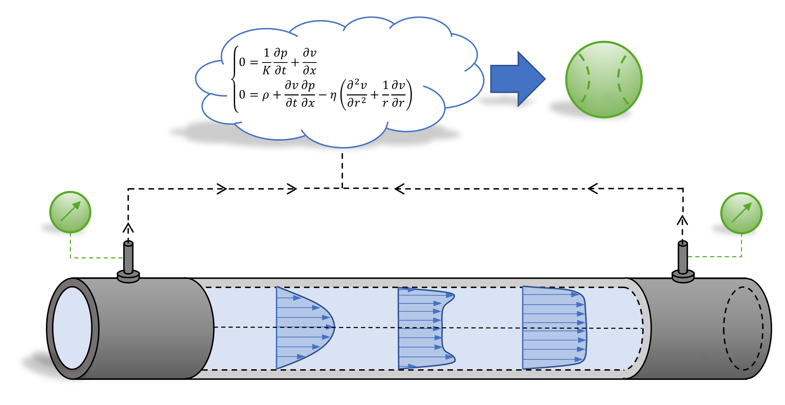
1. Introduction

Flow rate sensors are commonly employed in hydraulic engineering. Knowing the volumetric flow rate is critical for detecting leaks and monitoring the wear of system components in both stationary and mobile hydraulic systems. Additionally, in the emerging field of predictive maintenance, knowing flow rates and pressure levels allows for calculating power, efficiency, and potential losses.

There are two main issues with current volumetric flow sensors: First, most must be installed directly into the pipe, often using turbines or rotors, which disrupt the flow and increase system complexity. Second, the physical components of these sensors possess inertia, making them ineffective for measuring flows above a particular frequency. Pump pulsation measurements, for instance, become problematic, because they rely on flow sensors. The fundamental frequency of pump pulsations is influenced by the number of displacement units and the pump’s rotational speed. Pumps also produce pulsations at harmonic frequencies, many of which exceed the capabilities of most state-of-the-art sensors. These limitations highlight the need for new flow measurement methods. An ideal flow sensor would be non-invasive and accurately measure transient flow conditions. Ideally, it would operate as a soft sensor, relying solely on signals from other sensors, particularly pressure signals, which are often already available in fluid power systems.

The concept of calculating flow rates from pressure data is not new. Analytical methods for determining volumetric flow rates have been available since before the 1900s. One of the most well-known formulas is the Hagen-Poiseuille law (HP) [1], which calculates flow rates based on the friction-induced pressure drop within a pipe. However, this law is limited to steady, laminar flows and neglects the effects that become significant at higher frequencies. The so-called Richardson effect [2] alters the velocity profile at higher frequencies. Considering these factors, it is possible to derive an equation for transient flow rates consisting of the steady Hagen-Poiseuille solution with an added dynamic term. This paper will present an equation that led to the development of a soft sensor for transient volumetric flow rate computation based on pressure signals. Another significant contribution is by Zhao et al., who developed a method for measuring unsteady flow rates and velocities based on pressure differences, expressed through the transfer function between the mean flow velocity and the pressure gradient [3].

Hydraulic systems are often modeled analogously to electrical circuits, using resistances, inductors, and capacitances [4]. This approach is typically accurate and straightforward for many applications. However, at higher frequencies, system behavior changes due to transient effects. For instance, the characteristic impedance, propagation operators, and wall shear stress within pipes have all been shown to depend on frequency [5].

Recent advances in transient flow rate determination include work by Brereton et al., who presented a method for arbitrary transients in laminar pipe flow, starting from an initially steady state. This method relates the flow rate to the pressure-gradient history without making assumptions about velocity profiles [6]. In 2008, Brereton et al. introduced an indirect method that links flow rate to the centerline velocity history [7]. Sundstrom et al. [8] enhanced frictional modeling, reducing errors in flow rate calculations for the pressure-time method, a technique commonly used to measure discharge in hydraulic machinery. Foucault et al. proposed a method in 2019 for time-resolved transient flow rate calculation based on differential pressure measurements [9]. Their approach utilized the kinetic energy to predict specific laminar flow conditions well in real-time, relying only on two coefficients. García García et al. focused on unsteady turbulent pipe flow, validating their method through the transient response of the velocity field due to external perturbations, using a pressure step function as a test case [10]. Further investigations into turbulence were conducted by García García et al. in 2022, studying the transition from turbulent to laminar flow without an increase in bulk velocity. The observed laminarization was explained using a derived mathematical model [11].

Urbanowicz et al. conducted a comprehensive review of analytical models for accelerated incompressible Newtonian fluid flow in pipes. They examined different approaches with imposed pressure gradients and flow rates, focusing on their mathematical complexity and applicability to laminar and turbulent flows. Although existing models predict specific laminar flow conditions well, they struggle with turbulent flow scenarios [12].

In 2023, Urbanowicz et al. developed an analytical solution for modeling laminar water hammer events in pipes, validated through numerical simulations and experimental measurements [13]. Later that year, Urbanowicz et al. published new analytical models for wall shear stress in water hammer scenarios. By employing quasi-steady and transient hydraulic resistance assumptions, these models broadened the range of validity and simplified the mathematical descriptions. Explicit analytical expressions for wall shear stress during water hammer events were derived and numerically validated [14]. In two separate studies, Bayle et al. explored wave propagation models for water hammer events in pipes. The first paper developed a rheology-based model for viscoelastic pipes and validated it using experimental data [15], while the second study provided a wave propagation model in the Laplace domain applicable to a variety of boundary conditions in pipe scenarios [16].

This paper aims to implement a soft sensor by deriving an equation that accurately describes the volumetric flow rate in a pipe while considering the system’s higher-frequency behavior. This will be achieved by Laplace transforming (LT) the fundamental fluid mechanics equations, solving them in this domain, and then inverse Laplace transforming (ILT) them to obtain a solution in the time domain. The Laplace method has a prominent advantage over the Fourier domain since the solution obtained in the Laplace domain is valid for arbitrary pressure signals instead of only harmonic oscillating signals. The analytical model of the soft sensor exhibits two main benefits compared to currently available sensors and numerical solvers: High accuracy of transient compressible flow and real-time capability.

The subsequent section provides a brief presentation regarding the fluid mechanics fundamentals and the Laplace techniques. Afterward, the analytical model for the soft sensor is derived and investigated. A convolution of the derived solution is implemented to enable real-time application of the soft sensor, described in Sec. 3. The soft sensor is validated for several test cases, presented in Sec.3.2, and the results are shown in Sec. 4. Finally, a discussion of the results and a conclusion is given.

2. Materials and Methods

2.1. Law of Hagen and Poiseuille & Richardson Effect

Flow conditions can be characterized by the dimensionless Reynolds number, which gives a ratio between inertial and viscous forces. A Flow is laminar if the Reynolds numbers

R e = \frac{ρ v D}{η}

is below approximately 2300. Here,

ρ

is the density of the fluid, v is the axial fluid velocity, D is the pipe’s diameter and

η

is the dynamic viscosity. In this regime, the velocity profile across the pipe’s cross-section adopts a parabolic shape, with its vertex at the pipe center, and wave dissipation is disregarded. A critical aspect of this flow scenario is the no-slip condition at the pipe wall [17], which dictates that the fluid velocity at the wall is zero. Under these conditions, the Hagen-Poiseuille law [1] governs the flow:

Q = \frac{π R^{4}}{8 η L} Δ p = \frac{1}{R_{H}} Δ p

(1)

This formula provides the volumetric flow rate Q given the pressure difference

Δ p

, with

R_{H}

representing the hydraulic resistance, dependent on the pipe radius R, fluid viscosity

η

, and pipe length L. The relevance of hydraulic resistance will be explored further in later sections.

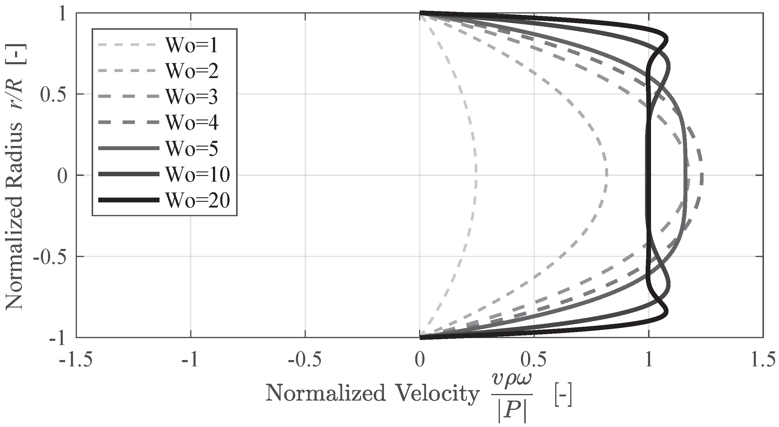
In 1929, Richardson [2] conducted experiments on unsteady airflow through a pipe generated by sinusoidal pressure fluctuations. Using a hot wire anemometer, he measured the radial velocity profile. He found that, within the laminar flow range of Reynolds numbers, increasing pressure frequencies caused the velocity profile to deviate from a parabolic shape, as shown in Figure 1. In this figure, the Womersley number

W o = R \sqrt{ω / ν}

is the root of the normalized frequency of the harmonically oscillating pressure input. It is based on the assumption of an incompressible fluid [5], where R is the pipe radius,

ν

the kinematic viscosity, and

ω

the pressure variation frequency.

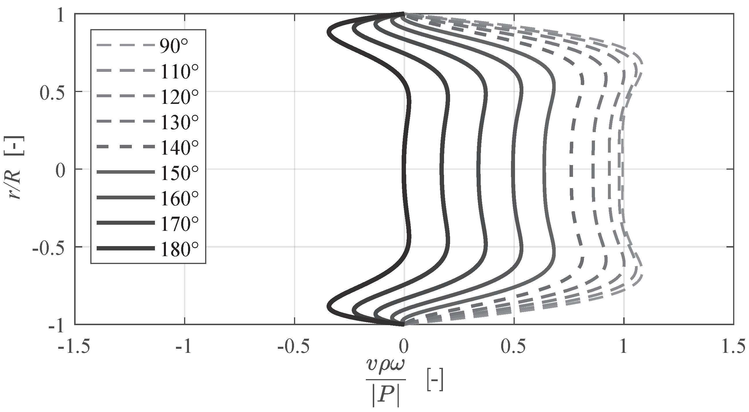
As the profile changes, it transitions to a flatter, more uniform shape in the center, with peaks near the wall and a sharp drop to zero at the boundary. This unsteady profile resembles those found in steady turbulent flows. Figure 2 illustrates the variation in the radial velocity profile over the phase of the harmonically oscillating pressure input for a Womersley number where the Richardson effect becomes apparent (

W o = 10

). The plot explicitly displays a quarter of the oscillation cycle of the input pressure.

Building on Richardson’s findings, Sexl [18] derived solutions for the instantaneous velocity profile as a function of the normalized radial position and the Womersley number. Stecki [5] performed the nondimensionalization of the axes in this context. The system equations developed in this paper allow for an analytical expression of the velocity profile transformation from parabolic to the one observed in Richardson’s experiments, thus extending the applicability of the presented equations beyond traditional laminar flow with a parabolic profile.

Since the early 20th century, various fluid behavior models have been developed, primarily from the fundamental Navier-Stokes equations. These models often incorporate simplifying assumptions to make them more computationally feasible [19,20,21,22]. Typical assumptions include liquid incompressibility, neglecting heat transfer effects, and the assumption of uniform pressure distribution across the pipe’s cross-section.

Stecki reviewed and categorized these models in his work [5,23], organizing them according to dimensionality and the effects considered. This paper’s general governing equations are those of the two-dimensional viscous compressible model. The volumetric flow rate equation is derived from this general framework.

2.2. Signal Processing Based on Laplace Techniques

Transforming functions from the time domain into the Laplace domain is a well-established technique in fields dealing with differential equations [24,25,26,27]. When this transformation is applied, all functions that depend on t are expressed in terms of s, where s is the Laplace variable. One key advantage of this approach is that time derivatives become simple multiplications by s, simplifying the differential equations. In the case of a differential equation that depends on one spatial operator and one temporal operator, the partial differential equation is reduced to an ordinary differential equation. Moreover, the Laplace transformation enables the analysis of arbitrary pressure signals, which is impossible with the Fourier method as it restricts solutions to harmonic, oscillating signals. This work aims to transform the system equations derived in the Laplace domain, back into the time domain, ultimately obtaining an accurate equation that links the flow to two pressure signals in the time domain.

One needs to perform an inverse Laplace transformation to revert from the Laplace domain to the time domain. The function must meet the necessary conditions for the existence of an ILT, notably that the function in the Laplace domain must converge to zero as

s \to \infty

. The ILT can be computed using a correspondence table after performing partial fraction decomposition for many Laplace domain functions. For example, Hsiao et al. calculated the hydrodynamic force and torque on a sphere using ILT techniques aided by integral tables [25]. However, in cases where partial fraction decomposition is not feasible and no correspondence table exists, a general formula is needed. This is provided by the Bromwich contour integral (eq. 2), which can be used to obtain the ILT of most functions [28]. In this transformation,

f (t)

and

F^{*} (s)

represent the same function in the time and Laplace domains, respectively, with

*

indicating the function in the Laplace domain. The poles of the function

F^{*} (s)

are denoted as

s = s_{j}

The Bromwich contour integral does not need to be directly computed in many cases. It can be evaluated indirectly using Cauchy’s contour integral, the Residue theorem from complex analysis, or numerical methods. For instance, Young et al. used a numerical approach to determine the ILT and obtain a solution for three-dimensional time-dependent circulation in shallow lakes [24]. Manhartsgruber conducted further work for instantaneous volumetric flow rates in circular pipes [26,27]. He utilized the fast inverse Laplace transformation (FILT) to obtain a representation of the physical signal. The FILT inherently contains a truncation error and limits the validity range of the determined result to instantaneous volumetric flow rates.

The Residue theorem’s advantage over numerical methods is that it provides an exact formula, offering more profound insight into the investigated system. Additionally, it extends the range of validity compared to numerically derived solutions and avoids concerns about numerical instabilities.

The integral over the complex plane is replaced by the sum of the residues of the function at its poles. Residues are specific coefficients found in the Laurent series expansion of a function around a pole [29]. It is worth noting that the Residue theorem is especially useful for dealing with functions that have complex poles.

All theorems and formulae referenced here can be found in the work by Krantz [29].

f (t) = \frac{1}{2 π i} \int_{β - i \infty}^{β + i \infty} e^{s t} F^{*} (s) d s = \sum_{j = 0}^{N} Res (e^{s t} F^{*} (s)) |_{s = s_{j}}

(2)

The residues for poles of order

m > 1

and

m = 1

are calculated using the general formula (eq. 3), which stems from the definition of the Laurent series.

Res (F^{*} (s)) |_{s = s_{j}} = lim_{s \to s_{j}} \frac{1}{(m - 1)!} \frac{d^{m - 1}}{d s^{m - 1}} [F^{*} (s) {(s - s_{j})}^{m}]

(3)

In the case of

m = 1

, and when the function is expressed as a fraction with

X^{*} (s)

as the numerator and

Y^{*} (s)

as the denominator, the residues for simple poles are calculated using eq. 4. The denominator is differentiated, and the entire term is evaluated at the simple poles

s = s_{k}

Res (F^{*} (s)) |_{s = s_{k}} = Res (\frac{X^{*} (s)}{Y^{*} (s)}) |_{s = s_{k}} = \frac{X^{*} (s_{k})}{\frac{\partial Y^{*} (s)}{\partial s} |_{s = s_{k}}}

(4)

For practical applications of these formulae, see Xie [30]. It is also crucial to remember that the product of two functions in the Laplace domain is equivalent to the convolution integral in the time domain [28]:

F^{*} (s) G^{*} (s) = f (t) * g (t) = \int_{0}^{t} f (t - τ) g (τ) d τ

(5)

Furthermore, the inverse Laplace transform (denoted as

L^{- 1}

) of a function multiplied by s is given by:

L^{- 1} \{s F^{*} (s)\} = \frac{\partial f (t)}{\partial t}

(6)

2.3. Analytical Model for Signal Processing of Pressure Transducer Signals

Generally, the Navier-Stokes equations govern fluid flow in three-dimensional space. However, solving the full Navier-Stokes equations is unnecessary for this case of liquid flow in a rigid pipe. A simplified version of the equations can be used to obtain a solution. The following assumptions are applied to simplify the Navier-Stokes equations:

The flow is laminar (Reynolds number $R e \leq 2300$ ), meaning the fluid layers do not mix. Consequently, the pressure remains constant across the pipe’s cross-section, and the pressure gradient in the radial direction is negligible.
Both the flow and pipe geometry are axisymmetric, resulting in no gradient in the angular direction, i.e., $(\frac{\partial}{\partial φ} = 0)$ .
The axial flow velocity $v_{x}$ is much smaller than the speed of sound a, which governs the fluid’s pressure wave propagation speed. Therefore, $v_{x} ≪ a$ , and the Mach number $M a = v_{x} / a ≪ 1$ , so supersonic effects can be ignored.
The pipe radius is much smaller than the pipe length ( $R ≪ L$ ), meaning no pressure reflections occur at the pipe walls.
The significant viscous effects in the motion equations are limited to those involving the radial distribution of axial velocity [5].
Gravitational forces are negligible as the pipe is horizontal, keeping the forces constant over its length.
Changes in fluid density due to vertical positioning are negligible because the pipe’s diameter is small.
Heat transfer is ignored since the focus is on liquids, excluding gases [31].

Using these assumptions, the Navier-Stokes equations can be simplified, and the general equation for the volumetric flow rate in the Laplace domain was derived in prior works [5,32]. The solution for the volumetric flow rate at the outlet of the pipe (

Q_{2}^{*}

) can be expressed as follows:

Q_{2}^{*} = \frac{1}{Z_{c} sinh (γ L)} p_{1}^{*} - \frac{coth (γ L)}{Z_{c}} p_{2}^{*} = W_{1}^{*} (ζ) p_{1}^{*} - W_{2}^{*} (ζ) p_{2}^{*} .

(7)

Inserting the definitions of the impedance

Z_{c}

and the propagation operator

γ

into the equation and multiplying both sides by

R_{H}

yields eq. 8.

Q_{2}^{*} R_{H} = \frac{8 D n \sqrt{I_{2} (\sqrt{ζ})}}{sinh [\sqrt{\frac{I_{0} (\sqrt{ζ})}{I_{2} (\sqrt{ζ})}} ζ D n] \sqrt{I_{0} (\sqrt{ζ})}} p_{1}^{*} - \frac{8 D n \sqrt{I_{2} (\sqrt{ζ})}}{tanh [\sqrt{\frac{I_{0} (\sqrt{ζ})}{I_{2} (\sqrt{ζ})}} ζ D n] \sqrt{I_{0} (\sqrt{ζ})}} p_{2}^{*} .

(8)

With:

\begin{matrix} γ L = \frac{s}{a} \sqrt{\frac{I_{0} (\sqrt{ζ})}{I_{2} (\sqrt{ζ})}} = s \frac{R^{2}}{ν} \frac{ν}{R^{2}} \frac{L}{a} \sqrt{\frac{I_{0} (\sqrt{ζ})}{I_{2} (\sqrt{ζ})}} = ζ D n \sqrt{\frac{I_{0} (\sqrt{ζ})}{I_{2} (\sqrt{ζ})}} . \end{matrix}

(9)

D n

is the dissipation number, which relates the time span of axial propagation of pressure waves to the radial diffusion of axial momentum, and

ζ

is the normalized Laplace variable defined as the following:

\begin{matrix} D n & = \frac{ν L}{R^{2} a} & ζ & = s \frac{R^{2}}{ν} \end{matrix}

(10)

Also,

R_{H}

is the hydraulic resistance introduced in Section 2.1. Note that

I_{n} (x)

is the modified Bessel function of the first kind of order n. In the later analysis of the ILT criteria, it became necessary to introduce an expansion factor of

ζ / ζ

to ensure all required criteria were satisfied. The denominator is incorporated into the weighting functions, while the numerator acts as a prefactor to the pressure. As a result, the time gradient of the pressures is considered in the time-domain equation rather than the pressures themselves.

Q_{2}^{*} R_{H} = W_{1}^{*} (ζ) \frac{ζ}{ζ} p_{1}^{*} - W_{2}^{*} (ζ) \frac{ζ}{ζ} p_{2}^{*}

(11)

Now, the

ζ

in the denominator will always be included in the weighting functions.

Q_{2}^{*} R_{H} = \frac{8 D n \sqrt{I_{2} (\sqrt{ζ})}}{sinh [\sqrt{\frac{I_{0} (\sqrt{ζ})}{I_{2} (\sqrt{ζ})}} ζ D n] ζ \sqrt{I_{0} (\sqrt{ζ})}} ζ p_{1}^{*} - \frac{8 D n \sqrt{I_{2} (\sqrt{ζ})}}{tanh [\sqrt{\frac{I_{0} (\sqrt{ζ})}{I_{2} (\sqrt{ζ})}} ζ D n] ζ \sqrt{I_{0} (\sqrt{ζ})}} ζ p_{2}^{*}

(12)

2.4. Inverse Laplace Transformation of the Weighting Functions for Compressible Fluids

Unlike in the incompressible case, for compressible fluids, the weighting functions of the pressures at both ends of the pipe are not equal due to the finite wave propagation speed. Therefore, each of the functions must be analyzed separately. The prefactors of the pressure functions from eq. 8 will be written as weighting functions:

\begin{matrix} W_{1}^{*} (ζ) = \frac{8 D n \sqrt{I_{2} (\sqrt{ζ})}}{sinh [\sqrt{\frac{I_{0} (\sqrt{ζ})}{I_{2} (\sqrt{ζ})}} ζ D n] ζ \sqrt{I_{0} (\sqrt{ζ})}}, \end{matrix}

(13)

\begin{matrix} W_{2}^{*} (ζ) = \frac{8 D n \sqrt{I_{2} (\sqrt{ζ})}}{tanh [\sqrt{\frac{I_{0} (\sqrt{ζ})}{I_{2} (\sqrt{ζ})}} ζ D n] ζ \sqrt{I_{0} (\sqrt{ζ})}} . \end{matrix}

(14)

Note the change from

sinh (x)

tanh (x)

, which effectively is only a multiplication of

W_{1}^{*}

with a

1 / cosh (x)

term. The weighting function

W_{1}^{*} (ζ)

for a fixed dissipation number

D n

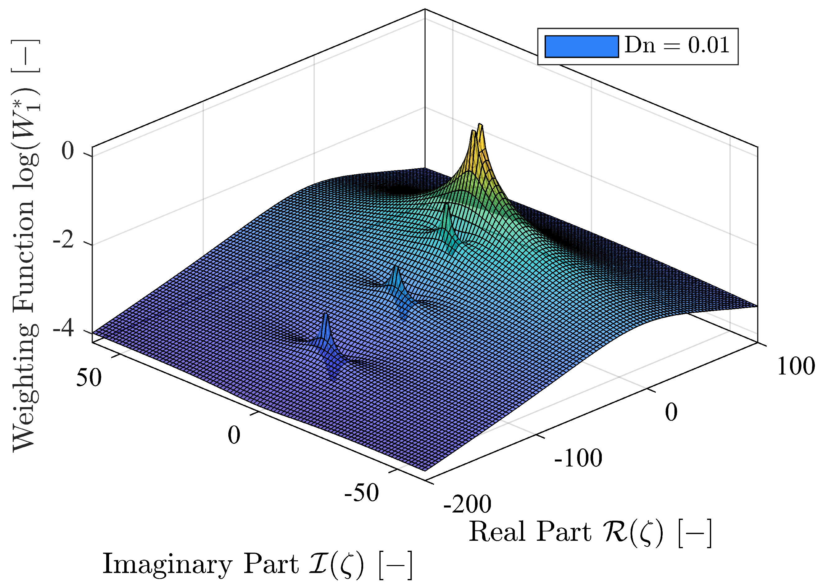
can be seen in Figure 3. Note the poles on the negative real axis starting from zero. For increasing values of

D n

, the poles would move further away from the origin.

2.5. Investigation of the Necessary Criteria for an ILT

First, the existence of the inverse Laplace transforms for the weighting functions must be established. To do this, it is essential that the limits of the weighting functions approach zero as

s \to \infty

and that the limits of the weighting functions multiplied by s remain finite as

s \to 0

. These conditions apply when using a normalized Laplace variable

ζ

instead of s. In what follows, the four required limits to confirm the existence of the inverse Laplace transforms for

W_{1}^{*} (ζ)

and

W_{2}^{*} (ζ)

will be examined. Firstly, the limits for

ζ \to 0

\begin{matrix} lim_{ζ \to 0} W_{1}^{*} (ζ) ζ \end{matrix}

(15)

\begin{matrix} = lim_{ζ \to 0} 8 D n \frac{\sqrt{I_{2} (\sqrt{ζ})}}{\sqrt{I_{0} (\sqrt{ζ})}} \frac{1}{sinh [\sqrt{\frac{I_{0} (\sqrt{ζ})}{I_{2} (\sqrt{ζ})}} ζ D n]} \end{matrix}

(16)

\begin{matrix} = lim_{ζ \to 0} 8 D n 1 \frac{1}{\infty} \end{matrix}

(17)

\begin{matrix} = lim_{ζ \to 0} \frac{8 D n}{\infty} = 0 \end{matrix}

(18)

\begin{matrix} lim_{ζ \to 0} W_{2}^{*} (ζ) ζ \end{matrix}

(19)

\begin{matrix} = lim_{ζ \to 0} 8 D n \frac{\sqrt{I_{2} (\sqrt{ζ})}}{\sqrt{I_{0} (\sqrt{ζ})}} \frac{1}{tanh [\sqrt{\frac{I_{0} (\sqrt{ζ})}{I_{2} (\sqrt{ζ})}} ζ D n]} \end{matrix}

(20)

\begin{matrix} = lim_{ζ \to 0} 8 D n 1 \frac{1}{1} = 8 D n \end{matrix}

(21)

Since

D n

must be finite, the overall limit must also be finite. Next, the two limits as

ζ \to 0

are evaluated.

\begin{matrix} lim_{ζ \to \infty} W_{1}^{*} (ζ) \end{matrix}

(22)

\begin{matrix} = lim_{ζ \to \infty} \frac{8 D n \sqrt{I_{2} (\sqrt{ζ})}}{sinh [\sqrt{\frac{I_{0} (\sqrt{ζ})}{I_{2} (\sqrt{ζ})}} ζ D n] ζ \sqrt{I_{0} (\sqrt{ζ})}} \end{matrix}

(23)

\begin{matrix} = lim_{ζ \to \infty} W_{1}^{*} (ζ) ζ lim_{ζ \to \infty} \frac{1}{ζ} \end{matrix}

(24)

\begin{matrix} = 0 \frac{1}{\infty} = 0 \end{matrix}

(25)

\begin{matrix} lim_{ζ \to \infty} W_{2}^{*} (ζ) \end{matrix}

(26)

\begin{matrix} = lim_{ζ \to \infty} \frac{8 D n \sqrt{I_{2} (\sqrt{ζ})}}{tanh [\sqrt{\frac{I_{0} (\sqrt{ζ})}{I_{2} (\sqrt{ζ})}} ζ D n] ζ \sqrt{I_{0} (\sqrt{ζ})}} \end{matrix}

(27)

\begin{matrix} = lim_{ζ \to \infty} W_{1}^{*} (ζ) ζ lim_{ζ \to \infty} \frac{1}{ζ} \end{matrix}

(28)

\begin{matrix} = 8 D n \frac{1}{\infty} = 0 \end{matrix}

(29)

The outcomes of these calculations confirm that all the required conditions for an inverse Laplace transformation are satisfied.

2.6. Approximation of the Hyperbolic Sine Term

In the following, the weighting function

W_{1}^{*}

will be examined, but it is important to note that the procedure for

W_{2}^{*}

is analogous to that for

W_{1}^{*}

. This can be inferred from eq. 12, as only the poles of a function and its zeros, located at the same positions as the poles, are relevant for an inverse Laplace transform (ILT). Since cosh does not introduce additional poles or zeros, all formulas applied to

W_{1}^{*}

can also be used for

W_{2}^{*}

W_{2}^{*} (ζ) = W_{1}^{*} (ζ) cosh [\sqrt{\frac{I_{0} (\sqrt{ζ})}{I_{2} (\sqrt{ζ})}} ζ D n]

(30)

With:

W_{1}^{*} (ζ) = \frac{8 D n \sqrt{I_{2} (\sqrt{ζ})}}{sinh [\sqrt{\frac{I_{0} (\sqrt{ζ})}{I_{2} (\sqrt{ζ})}} ζ D n] ζ \sqrt{I_{0} (\sqrt{ζ})}} .

(31)

The order of the poles of a function is crucial when calculating the residues needed for an ILT. To determine the order of the poles, we use an approximation for sinh from Goodson [33], as shown in eq. 32. This approximation is ideal because it is expressed as a product, preserving the poles’ properties and the function’s zeros. In contrast, Taylor series expansions do not maintain the poles and are thus unsuitable [34]. Increasing n in eq.32 corresponds to an increasing amount of complex zeros of the sinh term.

sinh (x) \approx {sinh}_{approx} (n, x) = x [\prod_{k = 1}^{n} (1 + \frac{x^{2}}{k^{2} * π^{2}})]

(32)

By inserting

n = 5

and

x = [\sqrt{\frac{I_{0} (\sqrt{ζ})}{I_{2} (\sqrt{ζ})}} ζ D n]

, eq. 32 becomes:

\begin{matrix} {sinh}_{approx} (5, [\sqrt{\frac{I_{0} (\sqrt{ζ})}{I_{2} (\sqrt{ζ})}} ζ D n]) = \sqrt{\frac{I_{0} (\sqrt{ζ})}{I_{2} (\sqrt{ζ})}} ζ D n (1 + \frac{I_{0} (\sqrt{ζ}) ζ^{2} D n^{2}}{(I_{2} (\sqrt{ζ}) π^{2})}) \\ (1 + \frac{I_{0} (\sqrt{ζ}) ζ^{2} D n^{2}}{(4 I_{2} (\sqrt{ζ}) π^{2})}) (1 + \frac{I_{0} (\sqrt{ζ}) ζ^{2} D n^{2}}{(9 I_{2} (\sqrt{ζ}) π^{2})}) (1 + \frac{I_{0} (\sqrt{ζ}) ζ^{2} D n^{2}}{(16 I_{2} (\sqrt{ζ}) π^{2})}) \\ (1 + \frac{I_{0} (\sqrt{ζ}) ζ^{2} D n^{2}}{(25 I_{2} (\sqrt{ζ}) π^{2})}) . \end{matrix}

(33)

It is important to note that the approximation

{sinh}_{approx} (5, x)

is equivalent to the standard "small angle" approximation of

sinh (x) = x

, which is derived from a truncated Taylor series and multiplied by the first five complex zeros of

sinh (x)

W_{1, app}^{*} (ζ) = \frac{8 D n \sqrt{I_{2} (\sqrt{ζ})}}{{sinh}_{approx} (5, x) ζ \sqrt{I_{0} (\sqrt{ζ})}}

(34)

With this approximation, the weighting function can be separated into the incompressible part

W_{inc}^{*} (ζ)

, which is derived using the small angle approximation of sinh for

D n \to 0

, and additional terms from the sinh approximation.

\begin{matrix} W_{1, app}^{*} (ζ) = & \frac{8 D n \sqrt{I_{2} (\sqrt{ζ})}}{{sinh}_{approx} (5, x) ζ \sqrt{I_{0} (\sqrt{ζ})}} \\ = & W_{inc}^{*} (ζ) \frac{1}{(1 + \frac{I_{0} (\sqrt{ζ}) ζ^{2} D n^{2}}{(I_{2} (\sqrt{ζ}) π^{2})}) (1 + \frac{I_{0} (\sqrt{ζ}) ζ^{2} D n^{2}}{(4 I_{2} (\sqrt{ζ}) π^{2})}) (1 + \frac{I_{0} (\sqrt{ζ}) ζ^{2} D n^{2}}{(9 I_{2} (\sqrt{ζ}) π^{2})})} \\ \cdot \frac{1}{(1 + \frac{I_{0} (\sqrt{ζ}) ζ^{2} D n^{2}}{(16 I_{2} (\sqrt{ζ}) π^{2})}) (1 + \frac{I_{0} (\sqrt{ζ}) ζ^{2} D n^{2}}{(25 I_{2} (\sqrt{ζ}) π^{2})})}, \end{matrix}

(35)

where

W_{inc}^{*} (ζ) = \frac{8 I_{2} (\sqrt{ζ})}{ζ^{2} I_{0} (\sqrt{ζ})}

. Note that

W_{inc}^{*} (ζ)

can be obtained by taking the limit of

{lim}_{D n \to 0} W_{1}^{*}

using

{lim}_{x \to 0} sinh (x) = {lim}_{x \to 0} tanh (x) = x

, which are the Taylor series approximations of the hyperbolic terms. Although

W_{1, app}^{*}

will not be used to compute the residues, it demonstrates that the complex poles of sinh are simple. With this information, the ILT can be computed from the residues of the function, which requires knowledge of the order and location of the poles. In conclusion, the weighting functions exhibit a double pole at

ζ = 0

, simple negative real poles from the incompressible part, and simple complex conjugate poles that depend on

D n

, which arise from the fluid’s compressibility effects.

2.7. Derivation of a Solution for a Fixed Dissipation Number for a Compressible Fluid

The previous chapter demonstrated that the poles of the weighting function depend on the dissipation number, making it impossible to derive a singular solution through an inverse Laplace transform (ILT) of the weighting function. This chapter derives the ILT for a fixed dissipation number of

D n = 0.0011

. This value is selected based on the pipe characteristics used in the test bench later in this project. Specifically,

D n = 0.0011

corresponds to a pipe length of

L = 1.5 m

, a diameter of

D = 14 mm

, and standard fluid properties of HLP46, including a density of

ρ = 860 kg / m^{3}

, a kinematic viscosity of

ν = 46 e - 6 m^{2} / s

, and a bulk modulus of

K = 14000 bar

The general formula for calculating residues, provided in Eq. 4, is now applied to determine the residue of the double pole at

ζ_{0} = 0

\begin{matrix} Res (W_{inc}^{*} (ζ)) |_{ζ_{0} = 0} = & lim_{ζ \to ζ_{0}} \frac{1}{(m - 1)!} \frac{d^{m - 1}}{d ζ^{m - 1}} [W_{inc}^{*} (ζ) {(ζ - ζ_{0})}^{m}] \\ \overset{m = 2}{=} & lim_{ζ \to ζ_{0}} \frac{d}{d ζ} [W_{inc}^{*} (ζ) {(ζ - 0)}^{2}] \\ = & lim_{ζ \to ζ_{0}} \frac{d}{d ζ} [W_{1}^{*} (ζ) ζ^{2}] \\ = & lim_{ζ \to ζ_{0}} \frac{d}{d ζ} [(\frac{8 I_{2} (\sqrt{ζ})}{ζ^{2} I_{0} (\sqrt{ζ})}) ζ^{2}] \\ = & lim_{ζ \to ζ_{0}} \frac{d}{d ζ} [\frac{8 I_{2} (\sqrt{ζ})}{I_{0} (\sqrt{ζ})}] \\ = & 1 \end{matrix}

(36)

The equation for the residues of simple, complex conjugated poles is given in eq. 5.

Res (W_{1}^{*} (ζ)) |_{ζ_{k}} = \frac{numerator [W_{1}^{*} (ζ_{k})] e^{ζ_{k} t_{n}}}{\frac{\partial}{\partial ζ} (denominator [W_{1}^{*} (ζ_{k})])}

(37)

The poles of the compressible component of the weighting function can be identified by solving

sinh [x] = 0

along with eq. 32. This leads to the following expression:

1 + \frac{I_{0} (\sqrt{ζ_{k}}) ζ_{k}^{2} D n^{2}}{k^{2} I_{2} (\sqrt{ζ_{k}}) π^{2}} = 0, for k \in N .

(38)

Rearranging for

ζ_{k}

, we obtain:

\frac{I_{0} (\sqrt{ζ_{k}}) ζ_{k}^{2}}{I_{2} (\sqrt{ζ_{k}})} = {(\frac{k π}{D n})}^{2} - 1 .

(39)

Assuming

D n = 0.0011

, the poles are located at:

$ζ_{1} = - 38.29545810 \pm 2818.211270 i$
$ζ_{2} = - 53.94617213 \pm 5658.549914 i$
$ζ_{3} = - 65.95601559 \pm 8502.531646 i$ .

When the first five complex poles and their conjugates are substituted into the formula for the residues Res, the resulting values are as follows:

\begin{matrix} W_{1, comp} & (t_{n}) = \\ - & (0.0000180 + 0.00270 i) e^{(- 38.30 - 2818.21 i) t_{n}} + (- 0.000018 + 0.00270 i) e^{(- 38.30 + 2818.21 i) t_{n}} \\ + & (0.0000066 + 0.00140 i) e^{(- 53.95 - 5658.55 i) t_{n}} + (0.0000066 - 0.00140 i) e^{(- 53.95 + 5658.55 i) t_{n}} \\ - & (0.0000036 + 0.00093 i) e^{(- 65.96 - 8502.53 i) t_{n}} + (- 0.0000036 + 0.00093 i) e^{(- 65.96 + 8502.53 i) t_{n}} \\ + & (0.0000023 + 0.00070 i) e^{(- 76.08 - 11348.4 i) t_{n}} + (0.0000023 - 0.00070 i) e^{(- 76.08 + 11348.4 i) t_{n}} \\ - & (0.0000016 + 0.00056 i) e^{(- 85.00 - 14195.4 i) t_{n}} + (- 0.0000016 + 0.00056 i) e^{(- 85.00 + 14195.4 i) t_{n}} . \end{matrix}

(40)

The curve-fitted ILT of the incompressible fluid is independent by Dn and is presented in Eq. 41:

\begin{matrix} W_{inc}^{*} (t_{n}) = 1 - 0.956788 e^{- 5.783 . t_{n}} - 0.03446 e^{- 30.4713 t_{n}} - 0.0006 e^{- 10^{1.5} t_{n}} \\ - 0.0076 e^{- 10^{2} t_{n}} - 0.0002 e^{- 10^{2.5} t_{n}} - 0.0005 e^{- 10^{3} t_{n}} . \end{matrix}

(41)

The normalized time

t_{n}

corresponding to the normalized Laplace variable

ζ

is:

\begin{matrix} t_{n} & = \frac{ν}{R^{2}} t . \end{matrix}

(42)

A subsequent paper will publish further details about the derivation of the incompressible model describing the volumetric flow rate calculation based on two pressure signals.

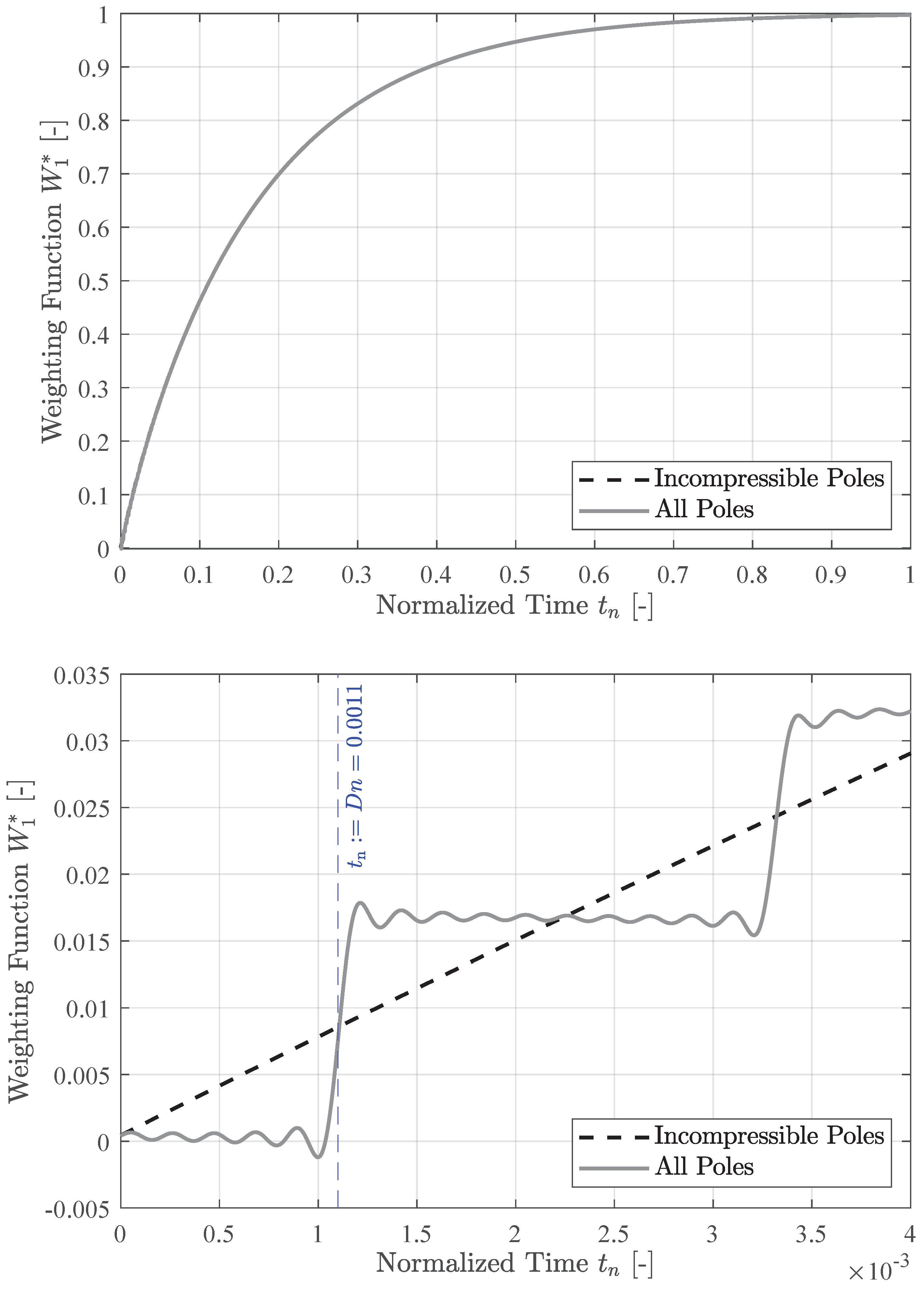
Combining both equations, we obtain the final expression for the volumetric flow rate in the time domain for a specified dissipation number. The impact of incorporating the compressible residues into the incompressible equation is illustrated in Figure 4.

The complex conjugate poles introduce a step function behavior in the weighting function, which is attributed to the fluid’s compressibility. During the time it takes for pressure information to travel from one end of the pipe to the other, the weighting function for that pressure must remain zero. This is emphasized in the figure by the vertical line marking the moment in time that corresponds to the selected dissipation number

D n

Notably, the dissipation number reflects the time required for the pressure to traverse the length of the pipe, expressed as

t_{n} = L / a

. It’s important to note that the vertical line at

t_{n} = D n

coincides with the first step increase, indicating the moment when pressure information reaches the far end of the pipe. This occurs regardless of the other variables defined in

D n

. Changes in the radius or kinematic viscosity of the fluid will also alter the normalized time in relation to

D n

Furthermore, as illustrated in Figure 4, the weighting function oscillates around zero instead of remaining at zero. This oscillation results from the approximation of the hyperbolic sine term. Including additional terms in the sine approximation would progressively smooth out the step functions with each added term.

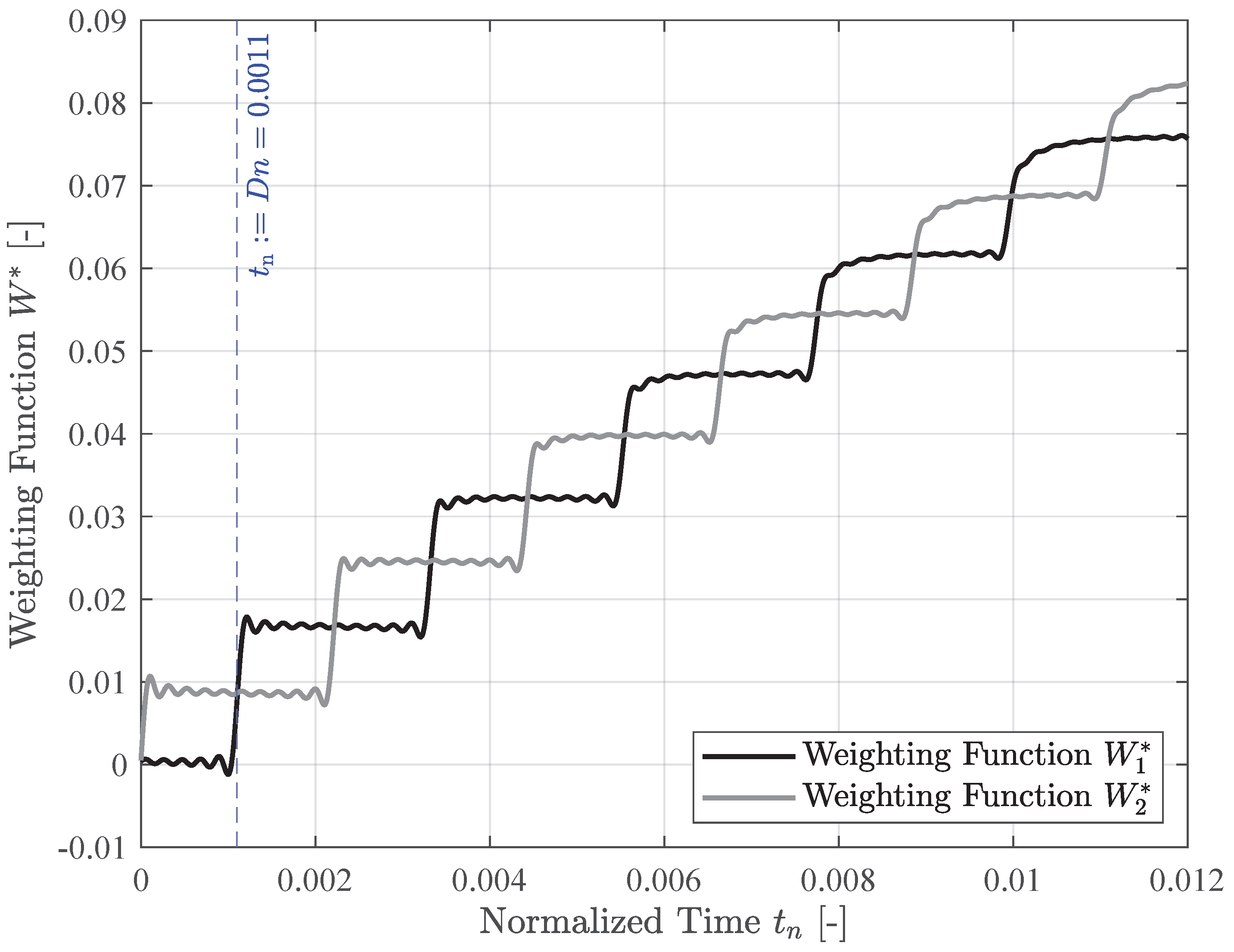
For completeness, the inverse Laplace transform (ILT) of the second weighting function,

W_{2}

, is shown in Figure 5 alongside the ILT of the weighting function

W_{1}

. These weighting functions are applied to the pipe’s corresponding pressures at both ends. Notably,

W_{2}

does not exhibit the delay time characteristic of the first weighting function, as pressure information at the second end of the pipe instantaneously influences the volumetric flow rate at that end.

2.8. Derivation of a Solution for Arbitrary Dissipation Numbers

As previously mentioned, the inverse Laplace transform (ILT) of the weighting function for both ends of the pipe in the case of an incompressible fluid is independent of the dissipation number

D n

and was presented in eq. 41. The primary challenge in determining the general ILT of

W_{1}^{*}

is that the poles depend on

D n

. The kth pole is indirectly defined by the following formula, derived from eq. 32 for

k > 0

1 + \frac{I_{0} (\sqrt{ζ_{k}}) ζ_{k}^{2} D n^{2}}{k^{2} I_{2} (\sqrt{ζ_{k}}) π^{2}} = 0 .

(43)

Rearranging for

ζ_{k}

yields:

\frac{I_{0} (\sqrt{ζ_{k}}) ζ_{k}^{2}}{I_{2} (\sqrt{ζ_{k}})} = {(\frac{k π}{D n})}^{2} - 1 .

(44)

Since it is not feasible to derive a solution applicable to all

D n

, the calculations will focus on discrete values of

D n

Using the software Maple [35], the first ten complex conjugate poles of the weighting functions were computed for dissipation numbers ranging from

1 e - 7

1 e - 1

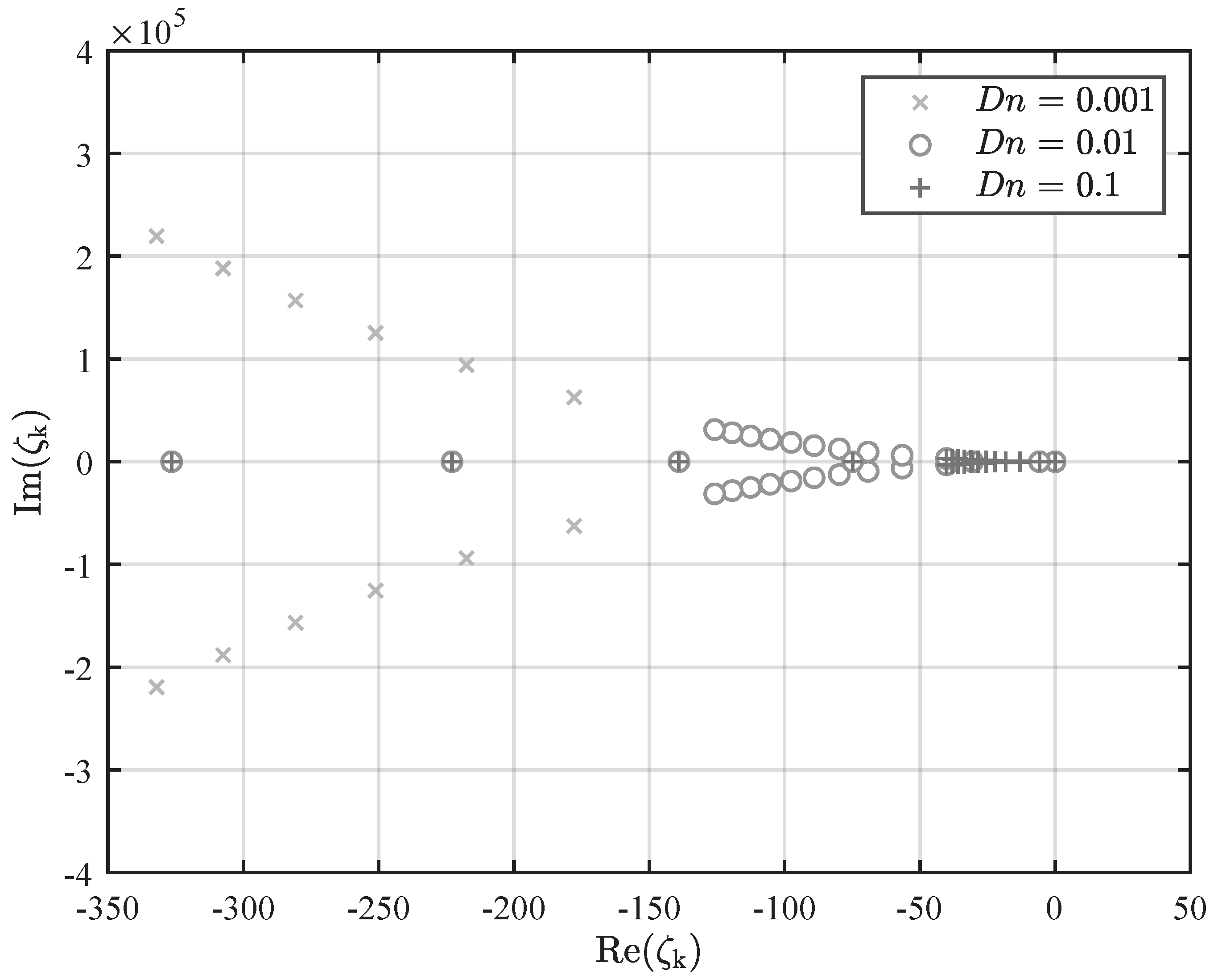
, with 100 increments per order of magnitude. This produced a matrix of dimensions 20 by 700. The positions of the poles in the complex plane for three different dissipation numbers are depicted in Figure 6. It can be observed that as the dissipation number decreases, the poles move further from the origin in the complex plane. Note that poles positioned further to the left on the negative half of the real axis correspond to faster-decaying residues, while those further away from zero on the imaginary axis are associated with faster-oscillating residues.

With the matrix of poles dependent on the dissipation number now in hand, we can calculate the residue for each pole across all considered dissipation number cases. The equation for the residues of simple poles is provided in eq. 45. Since all poles of the weighting function resulting from

sinh (x)

have been confirmed to be simple poles (as shown in eq. 35), this equation can be utilized for the automated computation of the residues:

Res (W_{1}^{*}) |_{ζ_{k}} = \frac{numerator [W_{1}^{*} (ζ_{k})] e^{ζ_{k} t_{n}}}{\frac{\partial}{\partial ζ} (denominator [W_{1}^{*} (ζ_{k})])} .

(45)

It is worth noting that in the exponent of

e

s_{k} t = s_{k} \frac{R^{2}}{ν} \frac{ν}{R^{2}} t = ζ_{k} \frac{ν}{R^{2}} t = ζ_{k} t_{n} .

(46)

We can compute a matrix containing all residues by utilizing Maple along with eq. 45. By combining this with the residues and poles from the incompressible case (as represented in eq. 41), we can obtain the weighting function in the time domain for discrete values of

D n

. The rounding of actual

D n

values to the nearest sampled values did not visibly impact the results.

3. Convolution of the Solution

In this chapter, the solution of the equation for volumetric flow rate in the time domain is evaluated. This involves a detailed examination of the convolution integral obtained as a solution, which will be simplified in this section.

To begin, we revisit eq. 12. For clarity, this equation is restated as eq. 47. To determine the volumetric flow rate in the time domain, we need to revert this equation into that domain:

Q_{2}^{*} R_{H} = W_{1}^{*} ζ p_{1}^{*} - W_{1}^{*} ζ p_{2}^{*} .

(47)

By applying the principle that the multiplication of two functions in the Laplace domain corresponds to the convolution of those same functions in the time domain, along with the fact that multiplying a function by the Laplace variable equates to taking the time derivative, we obtain:

Q_{2} (t_{n}) R_{H} = [\int_{0}^{t_{n}} W_{1} (t_{n} - τ) \frac{\partial p_{1} (t_{n} - τ)}{\partial t_{n}} d τ - \int_{0}^{t_{n}} W_{2} (τ) \frac{\partial p_{2} (t_{n} - τ)}{\partial t_{n}} d τ] .

(48)

Since the first term of both weighting functions is a constant, we can separate

W_{1}

and

W_{2}

, placing the constant term in a separate integral:

\begin{matrix} Q_{2} (t_{n}) R_{H} = & [\int_{0}^{t_{n}} 1 \frac{\partial p_{1} (τ)}{\partial t_{n}} d τ + \int_{0}^{t_{n}} (W_{1} (t_{n} - τ) - 1) \frac{\partial p_{1} (τ)}{\partial t_{n}} d τ] \\ - [\int_{0}^{t_{n}} 1 \frac{\partial p_{2} (τ)}{\partial t_{n}} d τ + \int_{0}^{t_{n}} (W_{2} (t_{n} - τ) - 1) \frac{\partial p_{2} (τ)}{\partial t_{n}} d τ] . \end{matrix}

(49)

It is practical to reorganize the equations into constant and dynamic components. The constant integral can be evaluated as the pressure difference given by

p_{1} (t_{n}) - p_{2} (t_{n}) = Δ p

\begin{matrix} Q_{2} (t_{n}) R_{H} = & [\int_{0}^{t_{n}} 1 \frac{\partial p_{1} (τ)}{\partial t_{n}} d τ - \int_{0}^{t_{n}} 1 \frac{\partial p_{2} (τ)}{\partial t_{n}} d τ] \\ + [\int_{0}^{t_{n}} (W_{1} (t_{n} - τ) - 1) \frac{\partial p_{1} (τ)}{\partial t_{n}} d τ - \int_{0}^{t_{n}} (W_{2} (τ) - 1) \frac{\partial p_{2} (τ)}{\partial t_{n}} d τ] \\ = & (p_{1} (t_{n}) - p_{2} (t_{n})) \\ + [\int_{0}^{t_{n}} (W_{1} (t_{n} - τ) - 1) \frac{\partial p_{1} (τ)}{\partial t_{n}} d τ - \int_{0}^{t_{n}} (W_{2} (τ) - 1) \frac{\partial p_{2} (τ)}{\partial t_{n}} d τ] \\ = & Δ p + [\int_{0}^{t_{n}} (W_{1} (t_{n} - τ) - 1) \frac{\partial p_{1} (τ)}{\partial t_{n}} d τ - \int_{0}^{t_{n}} (W_{2} (τ) - 1) \frac{\partial p_{2} (τ)}{\partial t_{n}} d τ] \end{matrix}

(50)

The resulting equation now contains a stationary term that resembles the Hagen–Poiseuille law

(Q R_{H} = Δ p)

alongside dynamic terms for each pressure function.

It is convenient to define the dynamic components of

W_{1}

and

W_{2}

as distinct dynamic weighting functions:

\begin{matrix} W_{1, dyn}^{'} & = W_{1} - 1, & W_{2, dyn}^{'} & = W_{2} - 1 . \end{matrix}

(51)

This leads to the expression:

Q_{2} (t_{n}) R_{H} = Δ p + [\int_{0}^{t_{n}} W_{1, dyn}^{'} (t_{n} - τ) \frac{\partial p_{1} (τ)}{\partial t_{n}} d τ - \int_{0}^{t_{n}} W_{2, dyn}^{'} (t_{n} - τ) \frac{\partial p_{2} (τ)}{\partial t_{n}} d τ] .

(52)

To clarify the impact of the dynamic components of the weighting functions, the negative signs from the summands of

W_{1, dyn}^{'}

and

W_{2, dyn}^{'}

are factored out and placed in front of the brackets:

Q_{2} (t_{n}) R_{H} = Δ p - [\int_{0}^{t_{n}} W_{1, dyn} (t_{n} - τ) \frac{\partial p_{1} (τ)}{\partial t_{n}} d τ - \int_{0}^{t_{n}} W_{2, dyn} (t_{n} - τ) \frac{\partial p_{2} (τ)}{\partial t_{n}} d τ] .

(53)

With:

\begin{matrix} W_{1, dyn} & = - W_{1, dyn}^{'}, & W_{2, dyn} & = - W_{2, dyn}^{'} . \end{matrix}

(54)

This outcome is reasonable since the Hagen–Poiseuille law describes an idealized flow condition that the equation aims to represent, specifically incompressible and steady flow rather than compressible unsteady flow. As HP represents an idealization, the actual flow rate must increase over time to match the value dictated by HP due to the effects of viscous friction.

3.1. Application of the TVB Method to Obtain the Soft Sensor

From a computational perspective, performing a full convolution of functions over the entire time range is impractical for the actual use of a soft sensor. Moreover, it is unnecessary, as the impact of pressure data diminishes over time, evidenced by the convergence of the weighting function to zero for large times. Vardy and Brown devised a method to compute convolutions efficiently between weighting functions and the time derivative of a discrete function [36]. This approach can similarly be applied to the convolution of a weighting function with a discrete function, as demonstrated in this paper. The weighting function is composed of exponential terms, and the discrete function is the difference between measured pressure signals.

The method’s efficiency lies in requiring only a few pressure data points while still delivering accurate results. The approach termed the "Trikha-Vardy-Brown" (TVB) method, is an extension of a convolution simplification method originally introduced by Trikha [37]. In 1975, Trikha proposed a one-step scheme for the convolution integral, incorporating historical acceleration into parameters updated at each integration time step [37]. However, Trikha’s method had two limitations: first, the historical component lacked the generality needed for different types of flows, and second, it was only valid for very small time steps, which was impractical for real-world applications.

In 1983, Kagawa et al. improved Trikha’s technique by deriving a model with ten exponential terms, in contrast to the previously used three [38]. Although this approach required more memory, it enhanced Trikha’s method. By 1991, Suzuki et al. had developed a hybrid model, combining full convolution for short durations with Trikha’s algorithm for longer times, using a sum of five exponential terms [39]. Later, Schohl proposed an enhanced stepping formula to correct the first-time step limitations of Trikha’s method. Assuming uniform acceleration, Schohl’s approach also employed five exponential terms [40]. Similarly, Vítkovský et al. improved the first-step accuracy by introducing an empirical decay factor and developed advanced exponential sum weighting functions applicable to both laminar and turbulent flows [41].

In 2002, Ghidaoui and Mansoor presented an alternative to Trikha’s one-step method by using a weighting function derived from the work of Vardy and Brown [42], which they employed to study the evolution of specific integrals in unsteady flow [43]. More recently, Urbanowicz refined Schohl’s method by correcting the erratic recursive formula used to compute unsteady wall shear stresses [44]. His results were validated using the computationally expensive formula from Vardy and Brown in 2010 [45].

In this contribution, the TVB method was implemented in Matlab [46]. The derivation follows the authors’ approach but is applied to the current equations.

The method is suitable for convolving a weighting function of the form

f (t) = \sum_{i = 1}^{N} m_{i} e^{- n_{i} t}

with the time derivative of a second function expressed as

g (t) = \frac{\partial p (t)}{\partial t}

Beginning with eq. 53, the flow rate can be divided into a stationary flow rate (according to the Law of Hagen and Poiseuille) and two dynamic flow rates corresponding to each pressure:

Q_{2} (t_{n}) = Q_{2, stat} (t_{n}) - [Q_{2, dyn, 1} (t_{n}) - Q_{2, dyn, 2} (t_{n})] .

(55)

The convolution integral for the stationary volumetric flow rate can be readily solved and is already presented in eq. 53. Consequently, the TVB method must be applied solely to the dynamic volumetric flow rates. The following derivation will exemplify this method for

Q_{2, dyn, 1}

, while the procedure for

Q_{2, dyn, 2}

would follow similarly.

As a starting point, the value of the integral evaluated up to the time

t_{n}

will be referred to as

Y_{0} (t_{n})

Q_{2, dyn, 1} (t_{n}) = \frac{1}{R_{H}} \int_{0}^{t_{n}} W_{1, dyn}^{*} (t_{n} - τ) \frac{\partial Δ p}{\partial t_{n}} (τ) d τ = \frac{1}{R_{H}} Y_{0} (t_{n}) .

(56)

Next of interest is the time step coming after

t_{n}

(t_{n} + Δ t_{n})

. Inserting into the equation gives:

Q_{2, dyn, 1} (t_{n} + Δ t_{n}) = \frac{1}{R_{H}} \int_{0}^{t_{n} + Δ t_{n}} W_{1, dyn}^{*} (t_{n} + Δ t_{n} - τ) \frac{\partial Δ p}{\partial t_{n}} (τ) d τ .

(57)

The complete integral will be divided into two parts: the integral from 0 to

t_{n}

, designated as

K_{1}

, and the integral from

t_{n}

t_{n} + Δ t_{n}

, referred to as

K_{2}

\begin{matrix} Q_{2, dyn, 1} (t_{n} + Δ t_{n}) & = \frac{1}{R_{H}} [K_{1} + K_{2}] \end{matrix}

(58)

With:

\begin{matrix} K_{1} & = \int_{0}^{t_{n}} W_{1, dyn}^{*} (t_{n} + Δ t_{n} - τ) \frac{\partial Δ p}{\partial t_{n}} (τ) d τ, \end{matrix}

(59)

\begin{matrix} K_{2} & = \int_{t_{n}}^{t_{n} + Δ t_{n}} W_{1, dyn}^{*} (t_{n} + Δ t_{n} - τ) \frac{\partial Δ p}{\partial t_{n}} (τ) d τ . \end{matrix}

(60)

First, the second part of the integral,

K_{2}

, will be evaluated.

K_{2}

represents the change in volumetric flow rate during the interval from the current time step to the next one, which is

Δ t_{n}

after the current step. Assuming a short time step, the change in the pressure gradient can be considered constant throughout the duration of

Δ t_{n}

. Thus, it follows that

\frac{\partial Δ p}{\partial t_{n}} (τ) = constant

for the entire period of

Δ t_{n}

. This allows the gradient to be factored out of the integral as a constant.

The constant value of the pressure difference gradient is determined by averaging over the time step, which involves taking the difference between the starting and ending values during the interval

Δ t

. Therefore:

Δ \dot{p} = {(\frac{\partial Δ p (τ)}{\partial t_{n}})}_{a v e r a g e d o v e r Δ t_{n}} .

(61)

Inserting this assumption into

K_{2}

gives:

K_{2} = Δ \dot{p} \int_{t_{n}}^{t_{n} + Δ t_{n}} W_{1, dyn}^{*} (t_{n} + Δ t_{n} - τ) d τ .

(62)

The weighting functions are recognized as a sum of weighted, falling exponential terms, which can be expressed as:

W_{d y n} (t_{n}) = \sum_{i = 1}^{N} m_{i} e^{- n_{i} t_{n}} .

(63)

Substituting this definition into the integral can be easily solved by integrating the exponential terms.

\begin{matrix} K_{2} & = Δ \dot{p} \int_{t_{n}}^{t_{n} + Δ t_{n}} [\sum_{i = 1}^{N} m_{i} e^{- n_{i} t_{n}}] d τ, \end{matrix}

(64)

\begin{matrix} K_{2} & = Δ \dot{p} \sum_{i = 1}^{N} \frac{m_{i}}{n_{i}} [1 - e^{- n_{i} (Δ t_{n})}] . \end{matrix}

(65)

Next, the first part of the integral, denoted as

K_{1}

, needs to be evaluated:

K_{1} = \int_{0}^{t_{n}} W_{1, dyn}^{*} (t_{n} + Δ t_{n} - τ) \frac{\partial Δ p}{\partial t_{n}} (τ) d τ .

(66)

In this context, the authors of the TVB method employed a Taylor expansion of the weighting function around the point

(t_{n} - τ)

. As a result,

K_{1}

becomes:

\begin{matrix} K_{1} \approx K_{1, a p p} = \int_{0}^{t_{n}} W_{d y n} (t_{n} - τ) \frac{\partial Δ p}{\partial t_{n}} (τ) d τ + Δ t_{n} \int_{0}^{t_{n}} {\frac{\partial W_{d y n}}{\partial t_{n}}|}_{(t_{n} - τ)} \frac{\partial Δ p}{\partial t_{n}} (τ) d τ \\ + \frac{{(Δ t_{n})}^{2}}{2!} \int_{0}^{t_{n}} {\frac{\partial^{2} W_{d y n}}{\partial t_{n}^{2}}|}_{(t_{n} - τ)} \frac{\partial Δ p}{\partial t_{n}} (τ) d τ + \dots . \end{matrix}

(67)

It is important to note that the subsequent derivatives of the weighting function take the form of:

\begin{matrix} \frac{\partial W_{d y n}}{\partial t_{n}} & = - n_{i} m_{i} e^{- n_{i} t_{n}}, \end{matrix}

(68)

\begin{matrix} \frac{\partial^{2} W_{d y n}}{\partial t_{n}^{2}} & = {n_{i}}^{2} m_{i} e^{- n_{i} t_{n}}, \end{matrix}

(69)

\begin{matrix} \frac{\partial^{3} W_{d y n}}{\partial t_{n}^{3}} & = - {n_{i}}^{3} m_{i} e^{- n_{i} t_{n}} . \end{matrix}

(70)

Due to this repetitive structure, the general derivative (of order k, where

k \in N

) can be expressed as:

\frac{\partial^{k} W_{d y n}}{\partial t_{n}^{k}} = - n_{i} \frac{\partial^{k - 1} W_{d y n}}{\partial t_{n}^{k - 1}} = C \frac{\partial^{k - 1} W_{d y n}}{\partial t_{n}^{k - 1}} = \dots = C^{k - 1} \frac{\partial W_{d y n}}{\partial t_{n}} .

(71)

Inserting these definitions of the derivatives of the weighting functions into the Taylor expansion yields:

K_{1, a p p} = \int_{0}^{t_{n}} W_{d y n} (t_{n} - τ) \frac{\partial Δ p}{\partial t_{n}} (τ) d τ [1 + C Δ t_{n} + \frac{{(C Δ t_{n})}^{2}}{2!} + \dots] .

(72)

Additionally, it is noteworthy that the first term in this equation is

Y_{0} (t_{n})

, as defined earlier.

K_{1, a p p} = Y_{0} (t_{n}) [1 + C Δ t_{n} + \frac{{(C Δ t_{n})}^{2}}{2!} + \dots] .

(73)

Interestingly, the terms within the brackets following

Y_{0} (t_{n})

resemble the series approximation of an exponential term with a factor C in the exponent. Consequently, the bracket can be rewritten as an exponential term instead (in this case,

C = n_{i}

K_{1, a p p} = Y_{0} (t_{n}) e^{C Δ t_{n}} = Y_{0} (t_{n}) e^{- n_{i} Δ t_{n}} .

(74)

Both integral parts are now simplified and can be substituted back into eq. 58:

\begin{matrix} Q_{2, dyn, 1} (t_{n} + Δ t_{n}) & = \frac{1}{R_{H}} [K_{1} + K_{2}], \\ Q_{2, dyn, 1} (t_{n} + Δ t_{n}) & \approx \frac{1}{R_{H}} \sum_{i = 1}^{N} [Y_{0, i} (t_{n}) e^{- n_{i} Δ t_{n}} + Δ \dot{p} \frac{m_{i}}{n_{i}} (1 - e^{- n_{i} Δ t_{n}})] . \end{matrix}

(75)

As a result, a one-step integration method for calculating the volumetric flow rate is established. For each step, the flow rate from the previous time step is multiplied by a decaying exponential term, effectively reducing its value. The current time step is then evaluated independently of any prior flow rate or pressure values and added to the diminished value from the last time step.

The significant advantage of this approach is that only the values from the previous time step need to be stored. In contrast, without this simplification, the entire convolution integral would need to be evaluated for each time step. Since the bounds of the convolution integral range from 0 to

t_{n}

, the length of the integral would increase indefinitely as time progresses, which would make the application of the soft sensor impracticable. With the implemented method the analytical model can be used offline and online on a real fluid power system to constantly measure the volumetric flow rate.

3.2. Test Cases

The following test cases are investigated to obtain a range of validity for the derived method. The volumetric flow rate obtained by the soft sensor is validated against the results provided by the software DSHplus, which solves the partial differential equations for the conservation of momentum and mass with a finite difference scheme [47]. The simulation model in DSHplus consists of a pipe with varying pressure inlet boundary conditions. Four different types of pressure signals are investigated: Sine, sum of sines, sawtooth, and step signals. In Table 1, the overall simulation parameters are displayed.

The comparison is done for a pipe with standard hydraulic oil HLP46 and a set diameter and length. Based on these values, the hydraulic resistance can be computed. The change between the different presented simulations lies in the investigated pressure boundary conditions. Table 2 displays the different types of investigated pressure boundary conditions. The pressure outlet is fixed; thus, only the pressure inlet varies.

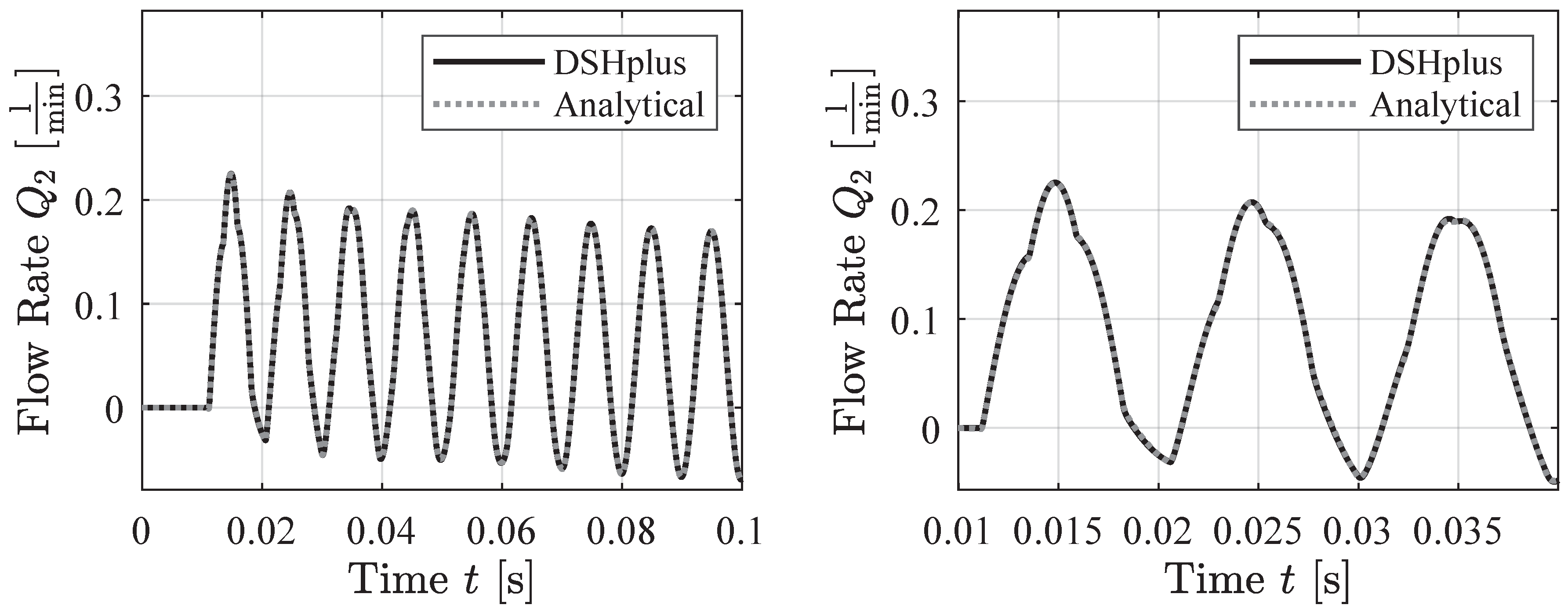
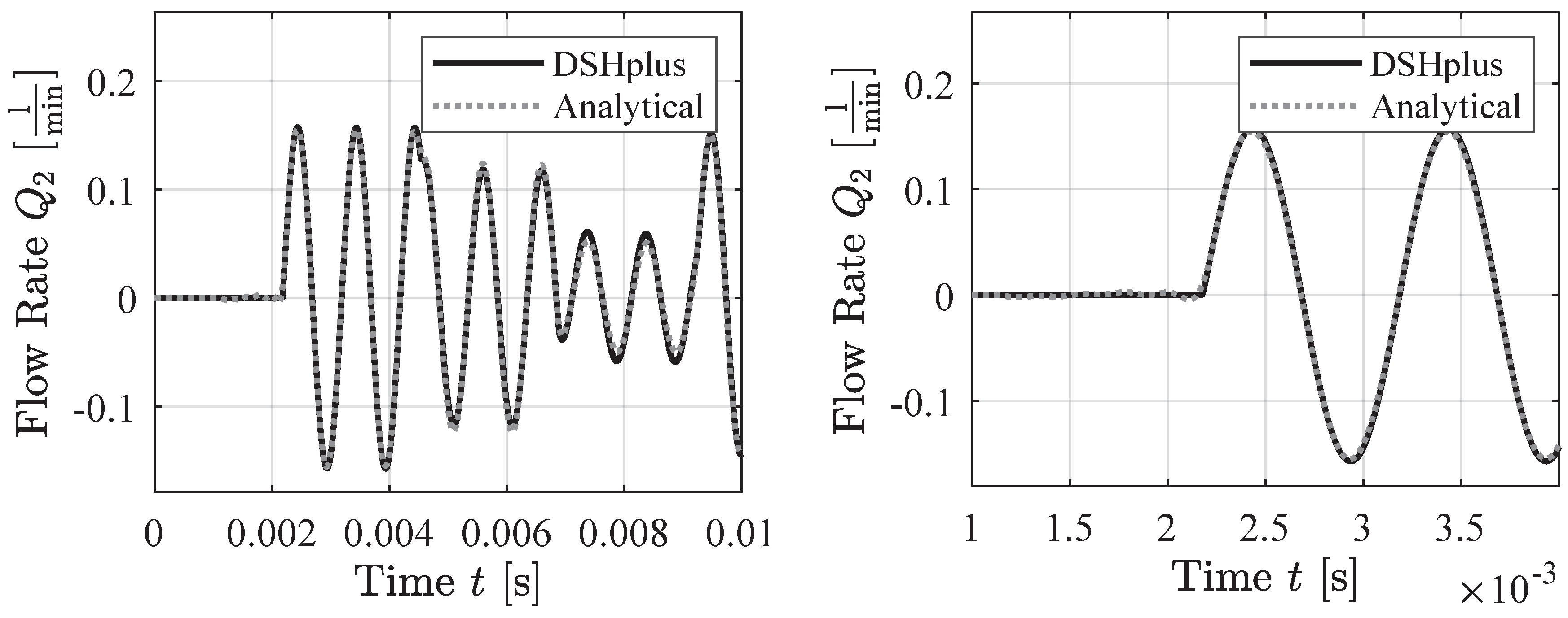
The first investigated pressure signals are sine waves at different frequencies (1, 100, and 1000 Hz) to validate the analytical model for low and high frequencies. When a pump delivers oil into a system, it inevitably generates pressure pulsations. These pulsations occur at a fundamental frequency determined by the number of chambers in the pump and its rotational speed. In addition, integer multiples of this fundamental frequency are also excited. To replicate this behavior, the pressure boundary condition for the simulations is defined as a sum of sine waves oscillating at 1 Hz, 10 Hz, 20 Hz, and 40 Hz, as well as 10 Hz, 100 Hz, 200 Hz, and 400 Hz Therefore, the second test case consists of two signals composed of sums of sines. Thirdly, a sawtooth function was examined as an example of a highly instationary boundary condition. Lastly, a step function was analyzed because this work focuses on the equation’s ability to calculate transient flow rates in a pipe. A step function increase in the pressure boundary condition will be examined to validate its performance under such conditions. A step function represents the most unsteady case possible, theoretically involving a Fourier approximation as a sum of frequencies up to infinity.

4. Results

4.1. Sine Wave Pressure Signals

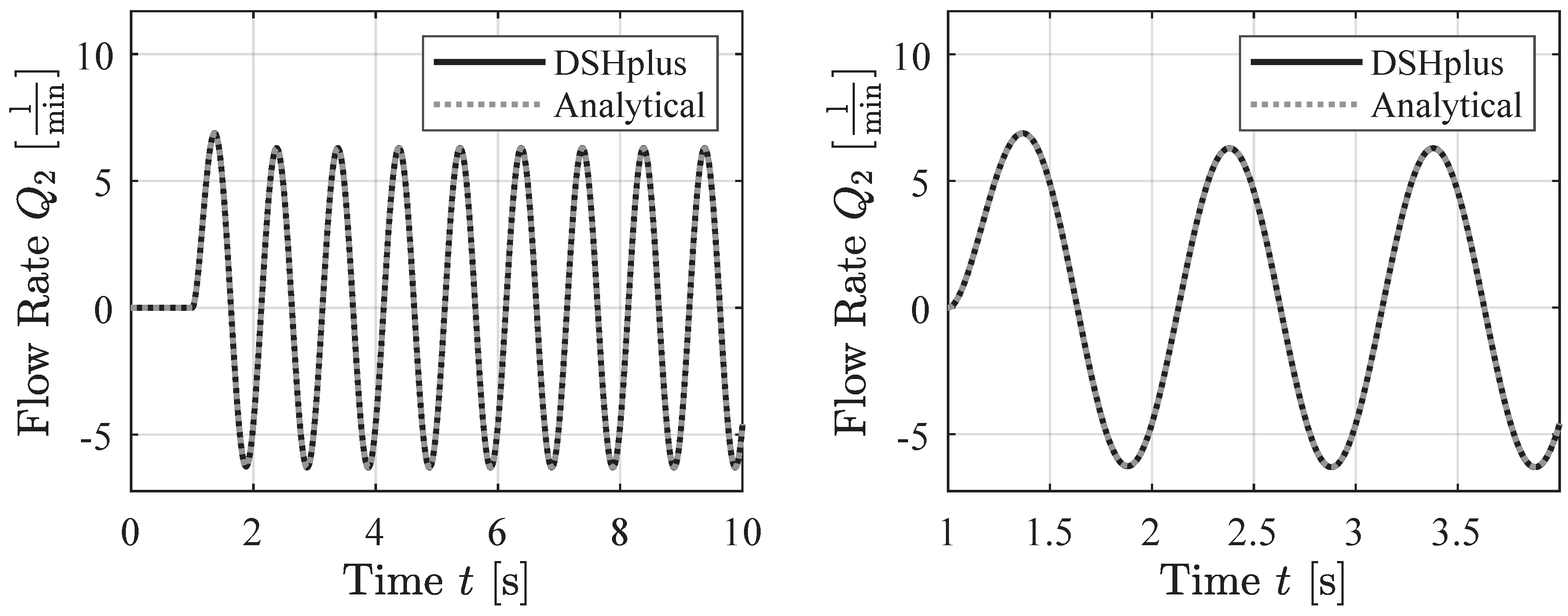
First, the analytical soft sensor is compared to the simulation data for cases involving sinusoidally varying pressure at one end of the pipe. Frequencies of 1 Hz, 100 Hz, and 1000 Hz were selected for the sine waves in Figure 7 to Figure 9. The analytical model shows good agreement with the simulation data in all cases.

4.2. Sums of Sine Wave Pressure Signals

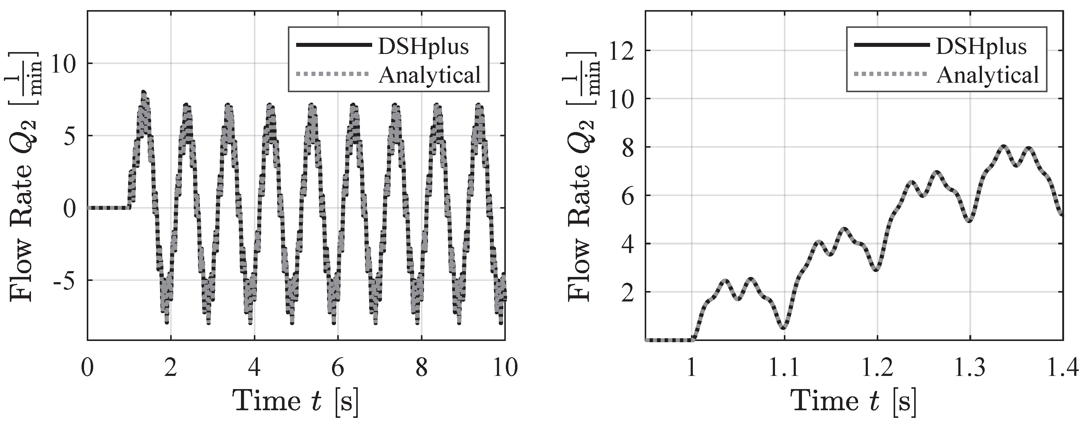
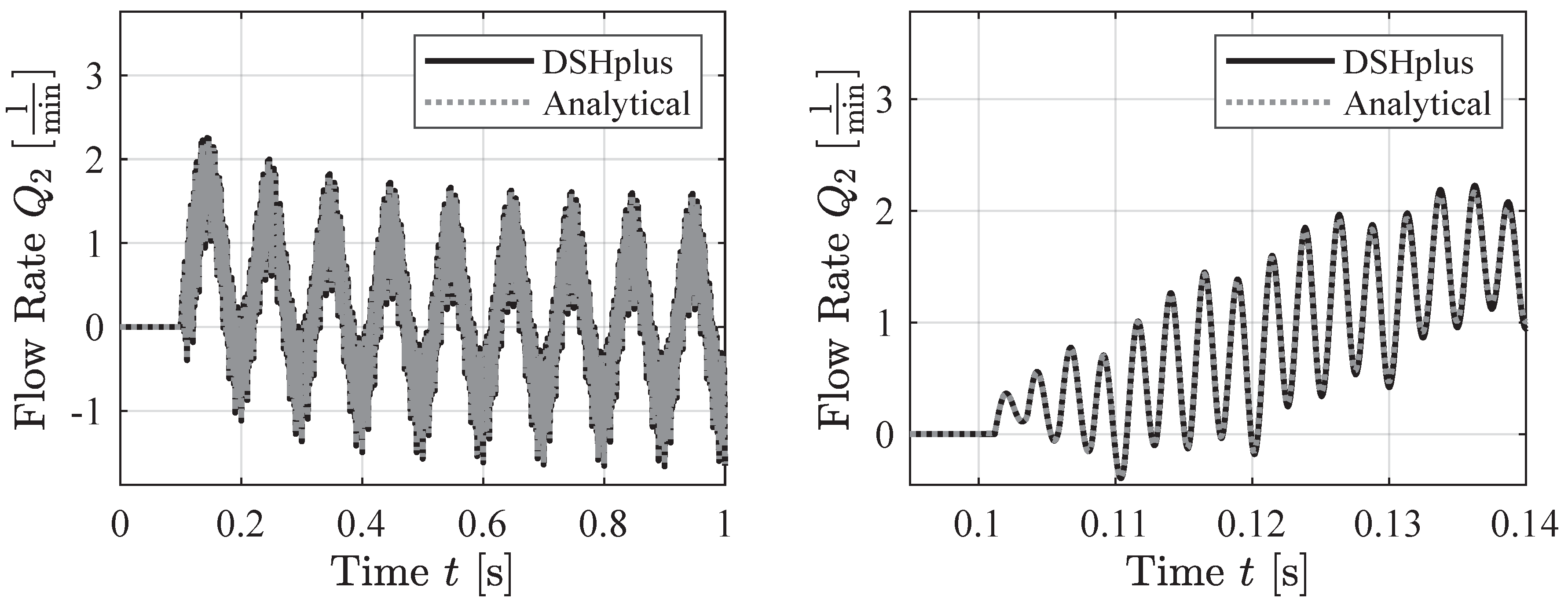
In the first following figure (Figure 10), the pressure boundary condition for the plots in this section is defined as a sum of sine waves oscillating at 1 Hz, 10 Hz, 20 Hz, and 40 Hz.

In the second following figure (Figure 11), the pressure boundary condition is set as a sum of sine waves at 10 Hz, 100 Hz, 200 Hz, and 400 Hz. Both figures demonstrate that the analytical model aligns well with the simulation data.

4.3. Sawtooth Pressure Signals

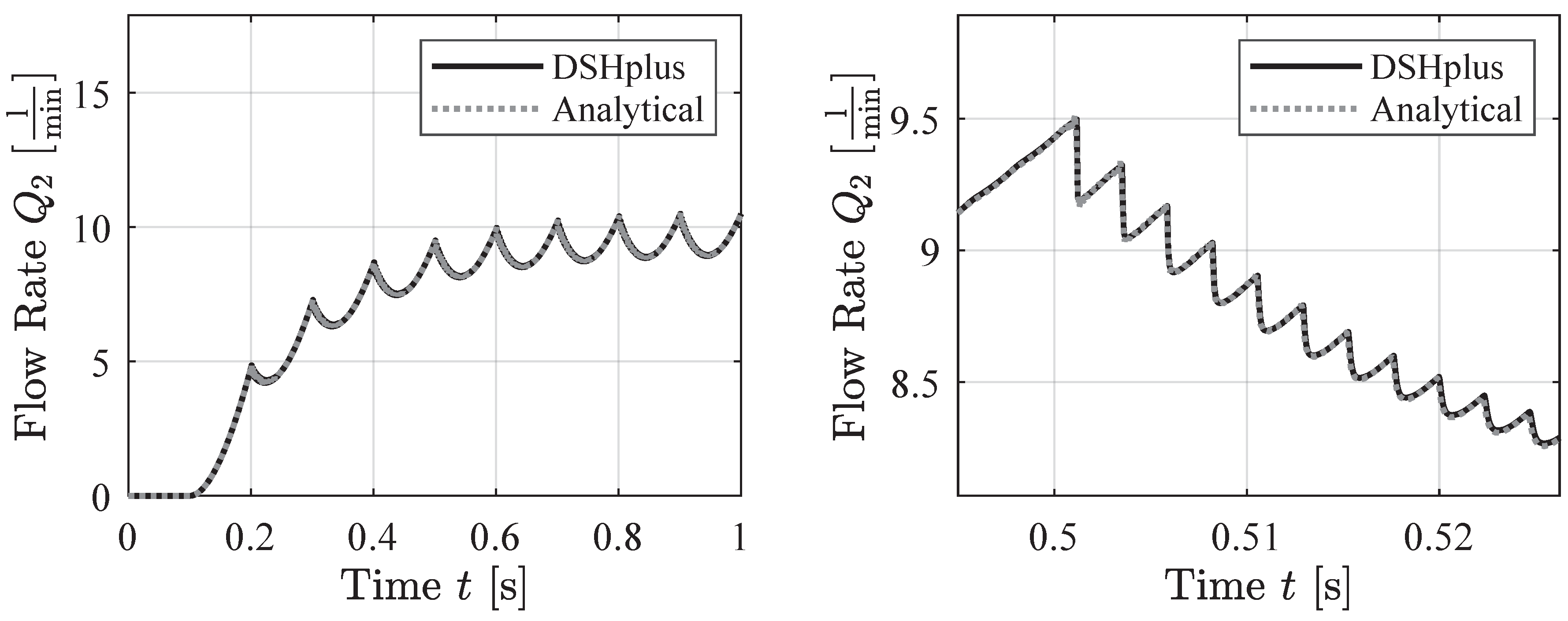
This section presents the agreement between the soft sensor and the simulation data for the case of sawtooth pressure boundary conditions. The figure below (Figure 12) displays a 10 Hz sawtooth wave. The soft sensor demonstrates good agreement with the simulation data. Additionally, the right plot in Figure 12 shows the compressible oscillations observed in the simulation data are also accounted for by the analytical model developed in this work.

4.4. Step Function Pressure Signal

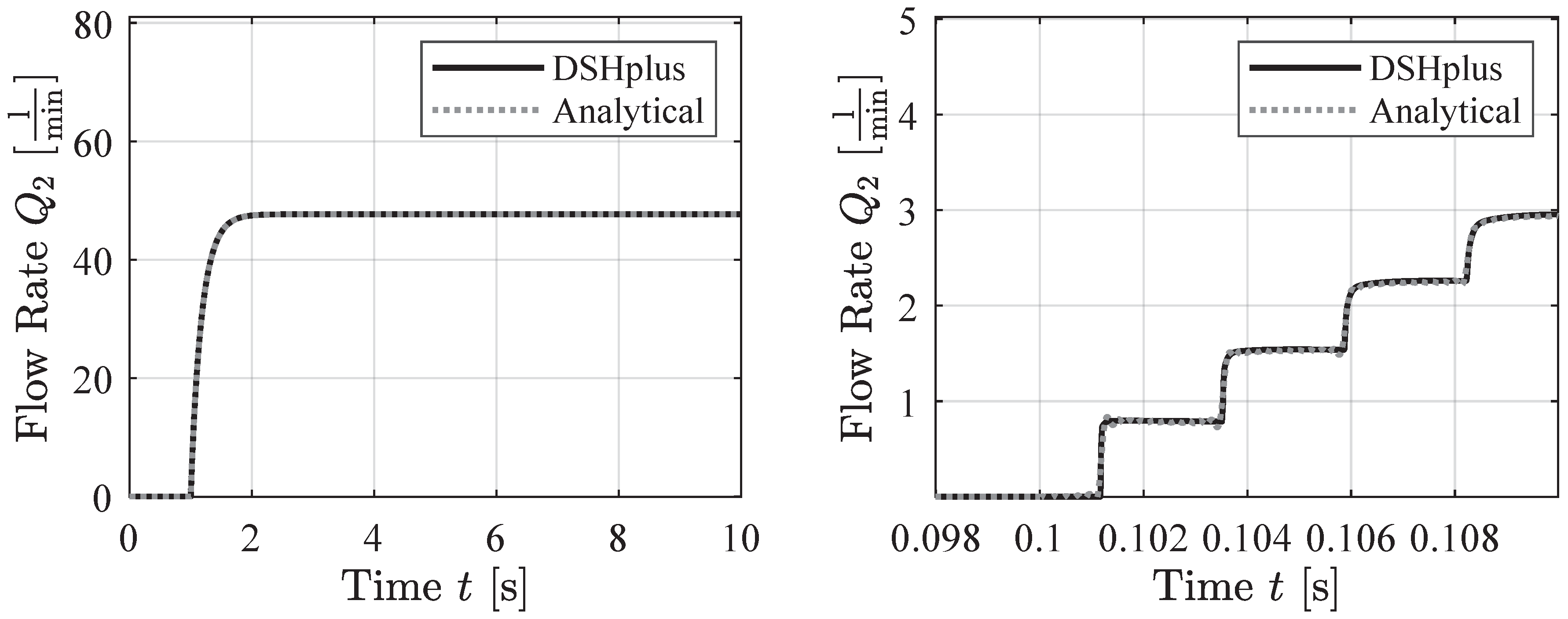
The two plots in Figure 13 display the same boundary condition at different zoom levels. The novel equation can capture the inductive behavior seen in the simulation data. Additionally, compressibility effects are evident in the step increases of the simulation data, and the equation reflects these step increments. As shown in Figure 13 on the right, the equation matches these steps through a Fourier approximation, oscillating around the constant values of the simulation data.

5. Discussion

The analytical soft sensor analysis based on two pressure signals revealed its promising ability to determine high-frequency flow rates. The model can accurately compute various flow rates with information about pressure signals. Due to its analytical nature, the computation is fast and not delayed due to numerical calculations compared to DSHplus. Nevertheless, the results obtained from the soft sensor display good agreement with the numerically computed values from the simulation model. The analytical model can accurately compute the correct flow rate for sine waves up to 1000Hz. Regarding the sum of sine waves, the model provides precise values for several overlaying sine waves. The same accuracy can be seen for the sawtooth test case and the step function. Noteworthy is that the step function contains a bandwidth of frequencies, which the analytical soft sensor accurately captures. Significantly, the investigation of the flow rate directly after the pressure step displays the ability of the model to capture compression phenomena, which are shown by the stair-like increase of the volumetric flow rate.

6. Conclusions

This contribution demonstrates the capability of an analytical soft sensor to determine compressible volumetric flow rates based on two pressure signals in a pipe. It starts with an introduction to current advances in the computation of transient flow rates, followed by a section regarding the fundamentals of fluid mechanics and the Laplace techniques to solve the governing equations to obtain an analytical model. Subsequently, the analytical model is presented, presenting the assumptions made and the inverse Laplace transformation, which transforms the examined equations. The developed model is investigated in the Laplace domain to obtain a deeper understanding, especially regarding its modeling of compressibility phenomena.

The soft sensor accurately computed the volumetric flow rate and was compared to numerically obtained results provided by the 1-D hydraulic simulation software DSHplus. Four test cases were investigated: Sine waves, sums of sine waves, sawtooth waves, and a step function to validate the soft sensor. The soft sensor agreed well with each test case’s numerically computed values. The soft sensor was able to determine even high-frequency flow rates of up to 1000 Hz and capture the compression phenomena visible in the step case.

The findings of this research present a significant advancement in soft sensors for transient flow rate measurement. This work introduces a novel method for obtaining precise and efficient volumetric flow rates in pipes by utilizing the Laplace techniques to solve the fundamental equations of fluid dynamics. This soft sensor consists of an analytical model that is both accurate and computationally efficient. Furthermore, the demonstrated precision at high frequencies and compressible flow conditions underscores the soft sensor’s potential for deployment in various industrial applications, such as condition monitoring and control, where real-time and accurate computation of crucial system parameters is essential. Additionally, the sensor’s ability to track pressure and flow rate enables the calculation of hydraulic power, which can be utilized for predictive maintenance, offering more profound insights into system performance. In contrast, traditional numerical solvers often provide either real-time solutions or high accuracy, but not both simultaneously due to the limitations inherent in numerical computation.

Future research will focus on extending the range of this soft sensor to turbulent flow and applying it to a real-world test rig [48] to validate its performance. Utilizing this soft sensor is a promising possibility to enhance the field of transient flow rate measurements. Furthermore, the effect of noisy pressure signals will be examined to improve the soft sensor’s robustness.

Author Contributions

Conceptualization, Faras Brumand-Poor, Tim Kotte, Enrico Pasquini and Katharina Schmitz; Data curation, Faras Brumand-Poor, Tim Kotte and Enrico Pasquini; Formal analysis, Faras Brumand-Poor, Tim Kotte and Enrico Pasquini; Funding acquisition, Faras Brumand-Poor and Katharina Schmitz; Investigation, Faras Brumand-Poor, Tim Kotte and Enrico Pasquini; Methodology, Faras Brumand-Poor, Tim Kotte and Enrico Pasquini; Project administration, Faras Brumand-Poor; Resources, Faras Brumand-Poor, Tim Kotte, Enrico Pasquini and Katharina Schmitz; Software, Faras Brumand-Poor and Tim Kotte; Supervision, Faras Brumand-Poor, Enrico Pasquini and Katharina Schmitz; Validation, Faras Brumand-Poor, Tim Kotte and Enrico Pasquini; Visualization, Faras Brumand-Poor and Tim Kotte; Writing – original draft, Faras Brumand-Poor and Tim Kotte; Writing – review & editing, Faras Brumand-Poor, Tim Kotte, Enrico Pasquini and Katharina Schmitz.

Funding

The IGF research project 21475 N / 1 of the research association Forschungskuratorium Maschinenbau e. V. (FKM), Lyoner Straße 18, 60528 Frankfurt am Main was supported by the budget of the Federal Ministry of Economic Affairs and Climate Action through the AiF within the scope of a program to support industrial community research and development (IGF) based on a decision of the German Bundestag.

Data Availability Statement

The data presented in this study are available on request from the corresponding author. The data are not publicly available due to privacy restrictions.

Conflicts of Interest

The authors declare no conflicts of interest.

Abbreviations

The following abbreviations are used in this manuscript:

FILT	Fast Inverse Laplace transformation
HP	Hagen-Poiseuille
ILT	Inverse Laplace transformation
LP	Laplace transformation
TVB	Trikha-Vardy-Brown

Nomenclature

Symbol	Definition	Unit
$*$	Denotation of a Variable in the Laplace Domain	[ $m^{2}$ /s]
a	Speed of Sound	[m/s]
C	Factor	[-]
D	Diameter of the Pipe	[m]
$D n$	Dissipation Number	[-]
$Δ p$	Difference in Pressure Between Inlet and Outlet	[Pa]
$Δ \dot{p}$	Averaged Pressure Over Time Step	[-]
$Δ t_{n}$	Normalized Time Step	[-]
f	Frequency	[Hz]
$f (t)$	Example Function	[-]
$F^{*} (s)$	Complex Example Function	[-]
$g (t)$	Example Function	[-]
$G^{*} (s)$	Complex Example Function	[-]
$I_{i}$	Modified Bessel function of the first kind of the i’th order	[-]
K	Bulk Modulus	[Pa]
$K_{1}$	First part of the convolution integral	[-]
$K_{2}$	Second part of the convolution integral	[-]
$K_{1, a p p}$	Approximation of $K_{1}$	[-]
k	A Natural Number	[-]
L	Length of the Pipe	[m]
m	Order of poles	[-]
$m_{i}$	Part of Assumed Weighting Function	[-]
$n_{i}$	Part of Assumed Weighting Function	[-]
N	Upper Limit of Residue Sum	[-]
$p_{B C, 1}$	Pressure Boundary Condition at Input Boundary	[Pa]
$p_{B C, 2}$	Pressure Boundary Condition at Output Boundary	[Pa]
$p_{I C, 1}$	Initial Pressure Condition at Input Boundary	[Pa]
$p_{I C, 2}$	Initial Pressure Condition at Output Boundary	[Pa]
$p_{1}^{*}$	Pressure at Inlet	[bar]
$p_{2}^{*}$	Pressure at Outlet	[bar]
Q	Volumetric flow rate	[ $m^{3}$ /s]
$Q_{i}$	Volumetric flow rate at Inlet: $i = 1$ and Outlet: $i = 2$	[ $m^{3}$ /s]
$Q_{i, d y n, j}$	Dynamic volumetric flow rate at port i caused by pressure at port j	[ $m^{3}$ /s]
$Q_{i, s t a t}$	Stationary volumetric flow rate at port i	[ $m^{3}$ /s]

Symbol	Definition	Unit
r	Radial Coordinate Within the Pipe	[m]
R	Radius of the Pipe	[m]
$R_{H}$	Hydraulic Resistance	[Pa/( $m^{3}$ /s)]
s	Laplace Variable	[-]
$s_{j}$	Poles of the Function $F^{*} (s)$	[Pa·s]
$s_{k}$	Simple Poles	[Pa·s]
${sinh}_{a p p r o x}$	Approximation of the $s i n h (s)$ Function	[-]
t	Time	[s]
$t_{n}$	Normalized Time	[-]
$τ$	Time	[s]
v	Axial Fluid Velocity	[v]
$v_{x}$	Axial Fluid Velocity	[v]
$W_{i}^{*}$	Weighting function at End $i \in {1, 2}$ of the Pipe	[-]
$W_{i, dyn}^{'}$	Dynamic Weighting function at port $i \in {1, 2}$	[-]
$W_{i, dyn}$	Negative of $W_{i, dyn}^{'}$	[-]
$W_{1, app}$	Weighting Function with Approximated sinh	[-]
$W_{comp}$	Compressible Weighting Function	[-]
$W_{inc}$	Incompressible Weighting Function	[-]
$W o$	Womersley Number	[-]
$X^{*} (s)$	Nominator of $F^{*} (s)$	[-]
$Y^{*} (s)$	Denominator of $F^{*} (s)$	[-]
$Y_{0}$	Integral at time step $t_{n}$	[-]
$ζ$	Normalized Laplace Variable	[-]
$ζ_{i}$	Poles of the Weighting Function	[Pa·s]
$Z_{c}$	Series impedance	[bar/( $m^{3}$ /s)]
$β$	Real Part of Bromwich Integral Boundaries	[-]
$η$	Dynamic Viscosity	[Pa·s]
$ν$	Kinematic Viscosity	[ $m^{2}$ /s]
$ω$	Pressure Variation Frequency	[1/s]

References

Sutera, S.P.; Skalak, R. The History of Poiseuille’s Law. Annual Review of Fluid Mechanics 1993, 25, 1–20. [Google Scholar] [CrossRef]
Richardson, E.G.; Tyler, E. The transverse velocity gradient near the mouths of pipes in which an alternating or continuous flow of air is established. Proceedings of the Physical Society 1929, 42, 1–15. [Google Scholar] [CrossRef]
Zhao, T.; Kitagawa, A.; Kagawa, T.; Takenaka, T. A Real Time Method of Measuring Unsteady Flow Rate and Velocity Employing Differential Pressure in a Pipe: Fluids Engineering. JSME international journal 1987, 30, 263–270. [Google Scholar] [CrossRef]
Schmitz, K.; Murrenhoff, H. Hydraulik, vollständig neu bearbeitete auflage ed.; Vol. 002, Reihe Fluidtechnik. U, Shaker Verlag: Aachen, 2018.
Stecki, J.S.; Davis, D.C. Fluid Transmission Lines—Distributed Parameter Models Part 1: A Review of the State of the Art. Proceedings of the Institution of Mechanical Engineers, Part A: Power and Process Engineering 1986, 200, 215–228. [Google Scholar] [CrossRef]
Brereton, G.J.; Schock, H.J.; Rahi, M.A.A. An indirect pressure-gradient technique for measuring instantaneous flow rates in unsteady duct flows. Experiments in Fluids 2006, 40, 238–244. [Google Scholar] [CrossRef]
Brereton, G.J.; Schock, H.J.; Bedford, J.C. An indirect technique for determining instantaneous flow rate from centerline velocity in unsteady duct flows. Flow Measurement and Instrumentation 2008, 19, 9–15. [Google Scholar] [CrossRef]
Sundstrom, L.R.J.; Saemi, S.; Raisee, M.; Cervantes, M.J. Improved frictional modeling for the pressure-time method. Flow Measurement and Instrumentation 2019, 69, 101604. [Google Scholar] [CrossRef]
Foucault, E.; Szeger, P. Unsteady flowmeter. Flow Measurement and Instrumentation 2019, 69, 101607. [Google Scholar] [CrossRef]
García García, F.J.; Fariñas Alvariño, P. On an analytic solution for general unsteady/transient turbulent pipe flow and starting turbulent flow. European Journal of Mechanics - B/Fluids 2019, 74, 200–210. [Google Scholar] [CrossRef]
García García, F.J.; Fariñas Alvariño, P. On the analytic explanation of experiments where turbulence vanishes in pipe flow. Journal of Fluid Mechanics 2022, 951, A4. [Google Scholar] [CrossRef]
Urbanowicz, K.; Bergant, A.; Stosiak, M.; Deptuła, A.; Karpenko, M. Navier-Stokes Solutions for Accelerating Pipe Flow—A Review of Analytical Models. Energies 2023, 16, 1407. [Google Scholar] [CrossRef]
Urbanowicz, K.; Jing, H.; Bergant, A.; Stosiak, M.; Lubecki, M. Progress in Analytical Modeling of Water Hammer. Journal of Fluids Engineering 2023, 145. [Google Scholar] [CrossRef]
Urbanowicz, K.; Bergant, A.; Stosiak, M.; Karpenko, M.; Bogdevičius, M. Developments in analytical wall shear stress modelling for water hammer phenomena. Journal of Sound and Vibration 2023, 562, 117848. [Google Scholar] [CrossRef]
Bayle, A.; Rein, F.; Plouraboué, F. Frequency varying rheology-based fluid–structure-interactions waves in liquid-filled visco-elastic pipes. Journal of Sound and Vibration 2023, 562. [Google Scholar] [CrossRef]
Bayle, A.; Plouraboue, F. Laplace-Domain Fluid–Structure Interaction Solutions for Water Hammer Waves in a Pipe. Journal of Hydraulic Engineering 2024, 150. [Google Scholar] [CrossRef]
Schröder, W. Fluidmechanik, 4., korrigierte auflage ed.; Vol. 16, Aachener Beiträge zur Strömungsmechanik, Wissenschaftsverlag Mainz: Aachen, 2018.
Sexl, T. Über den von E. G. Richardson entdeckten Annulareffekt. Zeitschrift fr Physik 1930, 61, 349–362. [Google Scholar] [CrossRef]
Brown, F.T. The Transient Response of Fluid Lines. Journal of Basic Engineering 1962, 84, 547–553. [Google Scholar] [CrossRef]
Womersley, J.R. Oscillatory flow in arteries: the constrained elastic tube as a model of arterial flow and pulse transmission. Physics in medicine and biology 1957, 2, 178–187. [Google Scholar] [CrossRef]
Catania, G.; Sorrentino, S. Dynamical analysis of fluid lines coupled to mechanical systems taking into account fluid frequency-dependent damping and non-conventional constitutive models: part 1 – Modeling fluid lines. Mechanical Systems and Signal Processing 2015, 50-51, 260–280. [Google Scholar] [CrossRef]
D’Souza, A.F. Dynamic response of fluid flow through straight and curved lines. Dissertation, Purdue University, Lafayette, USA, 1963.
Stecki, J.S.; Davis, D.C. Fluid Transmission Lines—Distributed Parameter Models Part 2: Comparison of Models. Proceedings of the Institution of Mechanical Engineers, Part A: Power and Process Engineering 1986, 200, 229–236. [Google Scholar] [CrossRef]
Young, F.D.L.; Liggett, J.A. Transient Finite Element Shallow Lake Circulation. Journal of the Hydraulics Division 1977, 103, 109–121. [Google Scholar] [CrossRef]
Hsiao, C.H.; Young, D.L. The singularity method in unsteady Stokes flow: hydrodynamic force and torque around a sphere in time-dependent flows. Journal of Fluid Mechanics 2019, 863, 1–31. [Google Scholar] [CrossRef]
Manhartsgruber, B. Instantaneous Liquid Flow Rate Measurement Utilizing the Dynamic Characteristics of Laminar Flow in Circular Pipes. In Proceedings of the ASME/JSME 2003 4th Joint Fluids Summer Engineering Conference. ASMEDC, 2003, pp. 159–164. [CrossRef]
Manhartsgruber, B. Instantaneous Liquid Flow Rate Measurement Utilizing the Dynamics of Laminar Pipe Flow. Journal of Fluids Engineering 2008, 130. [Google Scholar] [CrossRef]
Weber H., Ulrich, H. Laplace-, Fourier- und z-Transformation; Vieweg+Teubner Verlag: Wiesbaden, 2012. [CrossRef]
Krantz, S.G. Handbook of Complex Variables; Birkhäuser: Boston, MA, 1999. [Google Scholar]
Xie, C. Applications of Residue Theorem to Some Selected Integrals. Highlights in Science, Engineering and Technology 2024, 88, 452–457. [Google Scholar] [CrossRef]
Brown, F.T.; Nelson, S.E. Step Responses of Liquid Lines With Frequency-Dependent Effects of Viscosity. Journal of Basic Engineering 1965, 87, 504–510. [Google Scholar] [CrossRef]
Almondo, A.; Sorli, M. Time Domain Fluid Transmission Line Modelling using a Passivity Preserving Rational Approximation of the Frequency Dependent Transfer Matrix. International Journal of Fluid Power 2006, 7, 41–50. [Google Scholar] [CrossRef]
Goodson, R.E. Distributed system simulation using infinite product expansions. SIMULATION 1970, 15, 255–263. [Google Scholar] [CrossRef]
Goodson, R.E.; Leonard, R.G. A Survey of Modeling Techniques for Fluid Line Transients. Journal of Basic Engineering 1972, 94, 474–482. [Google Scholar] [CrossRef]
Maple 2019, 2019.
Vardy, A.E.; Brown, J.M. Efficient Approximation of Unsteady Friction Weighting Functions. Journal of Hydraulic Engineering 2004, 130, 1097–1107. [Google Scholar] [CrossRef]
Trikha, A.K. An Efficient Method for Simulating Frequency-Dependent Friction in Transient Liquid Flow. Journal of Fluids Engineering 1975, 97, 97–105. [Google Scholar] [CrossRef]
Kagawa, T.; Lee, I.; Kitagawa, A.; Takenaka, T. High Speed and Accurate Computing Method of Frequency-Dependent Friction in Laminar Pipe Flow for Characteristics Method. Transactions of the Japan Society of Mechanical Engineers Series B 1983, 49, 2638–2644. [Google Scholar] [CrossRef]
Suzuki, K.; Taketomi, T.; Sato, S. Improving Zielke’s Method of Simulating Frequency-Dependent Friction in Laminar Liquid Pipe Flow. Journal of Fluids Engineering 1991, 113, 569–573. [Google Scholar] [CrossRef]
Schohl, G.A. Improved Approximate Method for Simulating Frequency-Dependent Friction in Transient Laminar Flow. Journal of Fluids Engineering 1993, 115, 420–424. [Google Scholar] [CrossRef]
Vítkovský, J.; Stephens, M.; Bergant, A.; Lambert, M.; Simpson, A. Efficient and accurate calculation of Zielke and Vardy-Brown unsteady friction in pipe transients. In Proceedings of the 9th International Conference on Pressure Surges, Chester, United Kingdom, 03 2004.
Vardy, A.E.; Brown, J.M. Transient, turbulent, smooth pipe friction. Journal of Hydraulic Research 1995, 33, 435–456. [Google Scholar] [CrossRef]
Ghidaoui, M.S.; Mansour, S. Efficient Treatment of the Vardy–Brown Unsteady Shear in Pipe Transients. Journal of Hydraulic Engineering 2002, 128, 102–112. [Google Scholar] [CrossRef]
Urbanowicz, K. Fast and accurate modelling of frictional transient pipe flow. ZAMM - Journal of Applied Mathematics and Mechanics / Zeitschrift für Angewandte Mathematik und Mechanik 2018, 98, 802–823. [Google Scholar] [CrossRef]
Vardy, A.E.; Brown, J.M. Evaluation of Unsteady Wall Shear Stress by Zielke’s Method. Journal of Hydraulic Engineering 2010, 136, 453–456. [Google Scholar] [CrossRef]
The MathWorks Inc.. MATLAB version: 9.13.0 (R2022b), 2022.
FLUIDON GmbH. User Manual DSHplus 3.7,, 2007.
Brumand-Poor, F.; Schüpfer, M.; Merkel, A.; Schmitz, K. Development of a Hydraulic Test Rig for a Virtual Flow Sensor. In Proceedings of the Proceedings of the Eighteenth Scandinavian International Conference on Fluid Power (SICFP’23), 2023.

Figure 1. Laminar velocity profiles for various Womersley numbers ranging from 1 to 20. Adapted from [18]

Figure 2. Laminar velocity profiles for various Womersley numbers ranging from 1 to 20. Adapted from [18]

Figure 3. Logarithm of Absolute of Weighting Function

W_{1}^{*}

for Real and Imaginary Arguments for Fixed Dissipation Number

Figure 3. Logarithm of Absolute of Weighting Function

W_{1}^{*}

for Real and Imaginary Arguments for Fixed Dissipation Number

Figure 4. Weighting Functions Featuring: Only Residues of Negative Real Poles (Incompressible Solution) and Residues of All Poles (Compressible Solution)

Figure 5. ILT using Residue Theorem for Both Weighting Functions

Figure 6. Position of the Poles of

W_{1}^{*} (ζ)

for various

D n

Figure 6. Position of the Poles of

W_{1}^{*} (ζ)

for various

D n

Figure 7. 1 Hz Sine Wave Pressure Boundary at 50 bar Level

Figure 8. 100 Hz Sine Wave Pressure Boundary at 50 bar Level

Figure 9. 1000 Hz Sine Wave Pressure Boundary at 50 bar Level

Figure 10. Sum of Sine Waves with 1 Hz, 10 Hz, 20 Hz, and 40 Hz Pressure Boundary at 50 bar Level

Figure 11. Sum of Sine Waves with 10 Hz, 100 Hz, 200 Hz, and 400 Hz Pressure Boundary at 50 bar Level

Figure 12. Sawtooth Pressure Boundary at 50 bar Level

Figure 13. Step Function Pressure Boundary at 50 bar Level

Table 1. Parameter set in the simulation for each test case.

Name	Variable	Unit	Value
Kinematic Viscosity	$ν$	$m^{2}$ /s	$46 \cdot 10^{- 6}$
Fluid Density	$ρ$	kg/ $m^{3}$	860
Bulk Modulus	K	Pa	$14 \cdot 10^{9}$
Diameter of the Pipe	D	m	$14 \cdot 10^{- 3}$
Length of the Pipe	L	m	$1.5$
Hydraulic Resistance	$R_{H}$	Pa/( $m^{3}$ /s)	$6.294 \cdot 10^{7}$

Table 2. Pressure conditions set for each test case.

Test Case	Initial Conditions $p_{IC, 1, 2}$ [bar]	Boundary Conditions $p_{BC, 1}$ [bar]	Frequency f [Hz]
Sine	50	$50 \pm 0.1$	1, 100, 1000
Sum of Sines	50	$50 \pm [0.1, 0.1, 0.1, 0.1]$	[ $1, 10, 20, 40$ ], [ $10, 100, 200, 400$ ]
Sawtooth	50	$50 + 0, 2$	10
Step	50	$50 + 0.5$	N/A

Disclaimer/Publisher’s Note: The statements, opinions and data contained in all publications are solely those of the individual author(s) and contributor(s) and not of MDPI and/or the editor(s). MDPI and/or the editor(s) disclaim responsibility for any injury to people or property resulting from any ideas, methods, instructions or products referred to in the content.

© 2024 by the authors. Licensee MDPI, Basel, Switzerland. This article is an open access article distributed under the terms and conditions of the Creative Commons Attribution (CC BY) license (http://creativecommons.org/licenses/by/4.0/).

Copyright: This open access article is published under a Creative Commons CC BY 4.0 license, which permit the free download, distribution, and reuse, provided that the author and preprint are cited in any reuse.

Alerts

MDPI Initiatives

Important Links

Choose an area of interest and we will send you notifications of new preprints at your preferred frequency.

Disclaimer

Signal Processing for High-Frequency Flow Rate Determination: An Analytical Soft Sensor Using Two Pressure Signals

Abstract

Keywords:

Subject:

1. Introduction

2. Materials and Methods

2.1. Law of Hagen and Poiseuille & Richardson Effect

2.2. Signal Processing Based on Laplace Techniques

2.3. Analytical Model for Signal Processing of Pressure Transducer Signals

2.4. Inverse Laplace Transformation of the Weighting Functions for Compressible Fluids

2.5. Investigation of the Necessary Criteria for an ILT

2.6. Approximation of the Hyperbolic Sine Term

2.7. Derivation of a Solution for a Fixed Dissipation Number for a Compressible Fluid

2.8. Derivation of a Solution for Arbitrary Dissipation Numbers

3. Convolution of the Solution

3.1. Application of the TVB Method to Obtain the Soft Sensor

3.2. Test Cases

4. Results

4.1. Sine Wave Pressure Signals

4.2. Sums of Sine Wave Pressure Signals

4.3. Sawtooth Pressure Signals

4.4. Step Function Pressure Signal

5. Discussion

6. Conclusions

Author Contributions

Funding

Data Availability Statement

Conflicts of Interest

Abbreviations

Nomenclature

References

MDPI Initiatives

Important Links

Subscribe