
Submitted:
17 October 2024
Posted:
23 October 2024
You are already at the latest version
Abstract
In Antarctica, SAR interferometry was largely used in coastal glacial areas, while in rare cases this method was used on the Antarctic plateau. In this paper, the authors present a digital elevation and ice flow map based on SAR interferometry for an area encompassing Talos Dome (TD) and the Frontier Mountain (FM) meteorite site in North Victoria Land/Antarctica. A digital elevation model (DEM) was calculated using a double SAR interferometry method. The DEM of the region was calculated by extracting approximately 100 control points from the Reference Elevation Model of Antarctica (REMA). The two DEMs differ slightly in some areas, probably due to the penetration of the SAR-C band signal into the cold firn. The largest differences are found in the western area of TD, where the radar penetration is more pronounced and fits well with the layer structures calculated by the georadar and the snow accumulation observations. By differentiating a 70-day interferogram with the calculated DEM, a displacement interferogram was calculated that represents the ice dynamics. The resulting ice flow pattern clearly shows the catchment areas of the Priestley and Rennick Glaciers as well as the ice flow from the west towards Wilkes Basin. The ice velocity field was analyzed in the area of FM. This area has become well known due to the search for meteorites. The velocity field in combination with the calculated DEM confirms the generally accepted theories about the accumulation of meteorites over the Antarctic Plateau.
Keywords:
Antarctica
; Victoria Land
; Talos Dome
; Interferometry
; GNSS network
1. Introduction
In recent years, the availability of SAR satellite platforms has gradually increased with the Radarsat-2, Sentinel-1, TerraSAR-X and COSMO-SkyMed satellites [1,2,3,4,5]. In Antarctica, the availability of SAR imagery has greatly improved, but the availability of an extensive archive of the European Space Agency’s first Earth-observing satellite programme, consisting of two satellites, ERS-1 and ERS-2, as part of the VECTRA project (ESA-A.O. 3-108), still allows access to interferometric SAR data at very low cost. Since the study of the Antarctic plateau with SAR interferometry is rare in the literature [6], it was decided to conduct a pilot study on this method, initially using the historical ERS-1/2 SAR images. For this purpose, an area that had been intensively studied as part of the Italian research project in Antarctica (PNRA) was selected. The Talos Dome in North Victoria Land (see Figure 1) has been one of the best-studied sites in Antarctica since 2003 and is one of the best-known ice drilling sites in Antarctica. The main objective is to extract an ice core from a marginal dome of East Antarctica that dates back to the last two interglacial periods (about 250,000 years ago).
The project coordinating the measures is called TALDICE (The TALos Dome Ice CorE), a European ice core research project (Italy, France, Germany, Switzerland, United Kingdom) as part of the Italian Antarctic Programme (Programma Nazionale di Ricerche in Antartide). The aim of the research is to understand the mechanisms of climate change and to explain past, present and future climate trends. As part of this project, an extensive Radio Echo Sounding (RES) flight plan was carried out to identify the new drilling site [7,8]. The Frontier Mountains (FM) became an interesting area due to meteorites findings. Important work was carried out by Folco et al. (2002) [9] within the Italian ANTARTIDE programme based on satellite images, an airborne radar survey and ground work. Using these ground data, an attempt was made to interpret the differential interferometric SAR products as an interferometric DEM and the glacial flow velocities of a very large area. All data showed good integration with each other.
2. Methods and Database: The Synthetic Aperture Radar
Using images acquired by a synthetic aperture radar on board the ERS-1 and ERS-2 satellites, we were able to measure the regional velocity of the snow and ice surface using SAR interferometry. The principles of this technique are described in König et al. (2001) [10], Gabriel et al. (1989) [11] and Goldstein et al. (1993) [12], among others, and will not be repeated here. Unfortunately, there are no images suitable for SAR interferometry analysis for the area east of FM. Using the available images, the authors developed the digital elevation model presented here and an ice flow map covering an area of about 100 km by 100 km (Table 1).
First, all images were focalized using the focalization algorithms [12] to obtain the SAR magnitude images geocoded with the REMA-DEM, [13], see Figure 2.
Despite a relatively high phase noise, probably due to ionospheric disturbances, a digital elevation model (DEM) and the ice velocity field in the satellite’s line of sight were calculated for this area. The processing chain included the iterative co-registration of SAR images with sub-pixel accuracy, followed by the generation of interferograms and coherence images. The baselines were first estimated using Delft Precise Orbit data [14], and then refined. WGS-84 was used as the geodetic reference for creating the maps presented in this paper. It was found that the one-day and 70-day intervals had high coherence over the entire scene and therefore provided high quality phase fringes, allowing to successfully process the entire dataset of frames,see Table 1, which includes a list of the synthetic aperture radar scenes used in this study), The topographic phase was isolated by differencing the images I(1,2) from I(3,4) [15,16], assuming that the velocity field remains constant between the two images over the relevant period of 70 days (see Table 1). When combining normal baselines (Bn I(1,2) > Bn I(3,4)), it is assumed that the first tandem is much more sensitive to topography than the second and that the resulting topographic interferogram also represents a favorable baseline (121 m corresponding to 74 m elevation ambiguity) (Figure 3. The height ambiguity was resolved by phase-unwrapping. The derived DEM was then corrected using the REMA DEM as a digital reference elevation model to convert the topographic phase values into digital elevation values (Figure 3). In practice, the REMA DEM points were used as ground control points (GCP), taking into account only the points with high coherence. The GCP points were corrected using the EGM2008 global geoid model in order to obtain the heights on the WGS84 reference system [17].
However, the spatial distribution of the extracted GCPs was found to be sufficient for a correct calculation of the digital elevation model, allowing a least squares approach to minimize the difference between the calculated interferometric DEM and the GCPs extracted from the radar REMA DEM. The overall agreement proved to be reliable, as the maximum difference did not exceed 20 m. To improve the quality of the calculated DEM, the GCPs were removed over zones classified as highly penetrating for an electromagnetic signal and where the differences between the REMA DEM and the interferometric DEM are larger, e.g. in the Pristley Glacier area, although the results do not differ significantly apart from a generally smoother pattern of the interferometric DEM. The root mean square is very similar, which is probably due to the generally prevailing flat topography compensating for the fitting errors throughout the region (Figure 4).
3. Results
3.1. Talos Dome DEM and Magnitude Image Analysis
When comparing the two DEMs, it is noticeable that the general topographical pattern is very similar, with some differences. First, the REMA DEM “looks” smoother, while the ERS-SAR DEM is "noisier" due to phase noise. Comparing the two DEMs (Figure 5 and Figure 6), the trend of the topography in the Rennick Glacier is very similar, while in the FM area and along the Priestley Nevee’ the discrepancies are larger.
It is likely that the interferometric DEM in this area has similar accuracy and reliability, as the blue ice and bare ground in these areas have good reflectivity. In general, the differences between the two DEMs can be attributed to the different penetration depths that characterize the C-band in which the ERS-SAR radar operates [18], while the REMA DEM is a photogrammetric DEM that follows the optical surface. The C-band penetrates 10-20 meters into the ice, which means that the energy is not reflected from the surface of the ice but from the first ten meters below the surface [19,20,21,22,23].
According to Urbini et al. (2008) [7], the TD snow radar profile from GPR23 to GRP26 (positions in Figure 5) shows a layer located about 25 meters below the surface, which is consistent with the SAR signal penetrating a cold firn [18], with the same pattern visible in the 3D modeling of the GPR data. see Figure 7, which shows the interferometric coherence images using 70 days temporal delay.
Figure 6 shows the TD-GPR23 profile in which the profiles of the REMA-DEM, the digital interferometric terrain model and the GPR profiles of Layer 1 [7] are superimposed. The two profiles from radar and GPR are close to each other in the same area, but it is difficult to say whether the radar has a reflection corresponding to the same layer derived from the GPR. It is more likely that the reflection has a very large volumetric component.
Note that in the first 15 km the profiles almost overlap, corresponding to a zone of low accumulation, while between 15 and 30 km the profiles diverge and the radar signal shows considerable penetration, corresponding to an accumulation zone that is probably a more favorable environment for radar penetration, see Figure 8.
A comparison of Figure 7 and Figure 8 shows that the radar coherence corresponds to the areas of ice accumulation. Essentially, high coherence corresponds to areas of low accumulation, while low coherence corresponds to areas of high accumulation.
To summarize, the DEM SAR calculated from interferometry achieves good accuracy in rocky, blue and/or icy areas, but may not reflect the topographic surface in areas with good penetration. It is noted that the differences between the DEMs (Figure 5) are more or less randomly distributed, especially in the western area, while the eastern one shows a discrepancy between 10 and 25 meters below ground level, depending on the radar SAR penetration. The differences between the two DEMs can be interpreted as a mixture of three main sources of error:
- the penetration of the radar bands in cold firn;
- fitting errors associated with the ground control points (GCP) used to refine the interferometric baselines;
- phase noise resulting from differentiating the interferograms one or more times to remove the contribution of phase difference due to motion. Despite this significant error budget, the correlations between the REMA DEM and the interferometric DEM are high.
3.2. The Ice Flow Velocity Image
The interferometric computed ice surface velocity field of the ice surface in this area is between 0 and 0.010 m/day, which corresponds to a maximum of 0.004 m or 0.13 fringes/day in the satellite’s line of sight. This magnitude of displacement cannot be easily determined with tandem images (with a temporal baseline of one day). Therefore, the authors combined ERS-1 images from images 70 days apart as I(1,3) (Table 1) to increase the displacement component in the interferogram relative to the topographic component. The interferometrically derived DEM was used to simulate an interferogram with the same baseline as I(1,3) (139 m baseline), and then differentiated to obtain an interferogram representing only the motion component. A phase-unwrapping procedure was used to calculate the displacement that occurred between the 70 days apart images in the satellite’s line of sight (LOS). The movements were projected into their horizontal components. The derived ice velocity field was then converted into m/year values, see Figure 9.
The ice flow velocity structure derived from SAR interferometry provides additional information on the fine-scale structure of the ice flow pattern and on the probable regional sub-ice topography. The derivation of ice flow velocities by the SAR interferometry method only contains information about the direction of movement in the sense of “movement towards” the observing satellite" or “movement away” from it" [23]. It does not provide a fully consistent picture of the ice flow as it determines the extent of movement pixel by pixel. It is important to point out that the main limitation of this method is that the sensitivity tends towards zero when the glacier flow direction tends towards the perpendicular to the axis. Ice movements with an eastward component tend towards the blue color spectrum in Figure 8, while movements with a westward component tend towards the red color spectrum. Ice flow velocities of less than 0.2 m/year prevail over most of an area of almost 100 by 100 km. The ice flow pattern shows a radial outflow of ice from Talos Dome into areas with very little ice movement (white color in Figure 9 ), with the exception of an area in the east with an ice flow ≥ 1 m/year (blue colors in the eastern corner) towards the Rennick Glacier catchment. Also clearly visible is an accelerated ice flow towards the upper reaches of the Priestley Glacier catchment (blue color in the southern corner of Figure 9). The westward ice flow towards Wilkes Basin is shown in reddish colors. It is interesting that the area around TD has a very low velocity, which shows that the entire area of TD has a very low velocity pattern, which is typical for a dome zone. Interesting is the channeling of the velocity towards the Rennick glacier with negative velocity, indicating a "movement away" from the satellite. Since the one-dimensional velocity field does not clearly show the pattern of a "dome" of velocities as seen in Frezzotti et al. (2004) [8], this is due to both very low velocities (note that the velocities were calculated with images 70 days apart) and high phase noise due to volumetric scattering. Another unfavorable condition was the geometry of the SAR image, as the velocity component tends to zero in a southwest to northeast direction. For this reason, the points TD02, TD06, TD07, TD08 and TD09 obviously have a velocity of almost zero, see Figure 9. In addition, the geometry of the SAR image masks the components west of FM and east of TD. Very interesting is the velocity pattern in the areas -72.8, 157.1 and -72.8, 158.9 and -73.4, 159.6, where the largest outflows of the Priestley Nevee’ can be recognized. To estimate the velocities at points TD03, TD04 and TD05 (which are favorable from the point of view of the acquisition geometry), an estimate of the uncertainty of the glacier velocity measured along the slope was first made using the phase coherence, which determines the statistical noise of the interferometric phase [25]. Taking into account the coherence at points TD02, TD06, TD07, TD08 and TD09, which have low coherence and therefore a higher phase noise, the relative error is about 5 m/year in slant- range, which does not allow the estimation of velocities. Considering the vector components [7], projected from slant-range to ground-range, calculated along the GPS displacement vectors using the GPS heading values [8], along the maximum slope, the final value of the geometry favorable points are reported in Table 2.
Points TD03(INT) and TD04(INT) agree well with the GPS velocity estimate, while point TD05(INT) is only a rough velocity estimate, probably due to higher noise. Around the dome, the SAR coherence is quite high after 70 days and remains relatively high throughout the ice divide at east of TD. This corresponds to the areas of high slope. From Urbini et al. (2008) [7], when comparing the figures, it is easy to see that this area has lower storage and surprisingly corresponds to a zone of high SAR reflectance, probably due to a more compact stratification of the first 20-30 meters. From the same source this location has an accumulation of 60-70 kg m -2 yr -1, while in the west zone despite the velocity is kept very low coherence is low. This area corresponds to the areas with the largest accumulation of up to 110 kg m -2 yr -1 [7,24], and is probably more subject to volumetric scattering and therefore less coherence as the electromagnetic signal is more diffuse. To test the interferometric one-dimensional ice velocity map of the TD area, the two velocity components calculated with the MEaSUREs program were used [26]. This project was developed to collect multi-year digital records of Antarctic ice velocity. AIV products are created using proven, well-documented, peer-reviewed algorithms and numerical tools that have been refined over decades. However, besides the advantage of a two-dimensional velocity field, there is a lower resolution compared to the velocity field calculated with SAR interferometry, as the resolution is 450 m in both directions, while the resolution of the geocoded INSAR products is 20 m. It also shows that the TD is located in a low velocity zone and the dome-shaped velocity field can be better understood compared to a one-dimensional velocity field. Furthermore, using 70-day SAR images (without the topography component), the velocity field is much more sensitive to low velocities as they occur in the Antarctic plateau regions. In addition, the velocity field in the Frontier mountain area does not seem to be such that the glacier flow can be analyzed in detail, even if it shows that it is a low velocity area. Therefore, the velocity field presented in this paper seems to be better overall, although it is only one-dimensional.
3.3. The Frontier Mountain Area
Figure 10, of the FM area shows ice movements in the order of dm/year to m/year, values compatible with point measurements of ice flow by Folco et al. (2002) [9]. The ice divide was constructed based on the detailed DEM (Figure 5) and its position differs slightly from the position shown in Folco et al. (2002) [9]. The other positions of the ice-divide are in according with those of Folco et al. (2000) [27].
A close-up of the FM region (Figure 10) shows average ice flow velocities of m/year or less over much of the blue ice area north of FM (meteorite concentration site) in good agreement with previous ground-based measurements [9]. Frezzotti et al. (2004) [8] have shown that this is due to the sublimation of the wind blowing SW-NE, which also contributes to the NW-SE elongated shape of the dome, making the surface and subsurface more compact and thus more reflective of the radar signal. This is also confirmed by radar altimeter measurements. Changes in surface elevation in the vicinity of TD can be derived from an altimeter dataset collected over a period of eight years [24]. The entire region around FM is characterized by varying degrees of ice level lowering (Figure 7). The largest ice level declines are clearly associated with the Rennick and Priestley Glacier catchments. The analysis shows an annual elevation decline of 3 to 7 cm per year for the FM area.
The Frontier Mountain (FM) area is an area where a large number of meteorites have been discovered. There are numerous papers in the literature that focus on glaciological reasons that can be used to explain such a phenomenon [9,28,29,30,31,32,33]. Figure 10 shows an idealized map of the Frontier Mountain in relation to the most important meteorite concentration sites superimposed with an interferometric ice velocity map. The location ”Meteorite Valley“ is labeled M-MV, the meteorite concentration on the blue ice is labeled M-BI [9], A detailed investigation based on satellite imagery, an airborne radar survey and ground work around the FM site by Folco et al. (2002) [9] has greatly improved our insight into the details of the meteorite concentration process taking place. The physiographically determined FM is located at the easternmost edge of an extension of a plateau of the Antarctic interior, over which TD rises. The InSAR-derived velocity map confirms the earlier observation by Folco et al. (2002) [9] and Delisle et al. (1989) [34] that FM is located near the ice divide between the catchments separating the ice flow to Priestley Glacier on one side and Rennick Glacier on the other. Figure 10 shows the ice flow pattern derived by SAR interferometry for the same region as in Figure 9. The ice movements have an eastward component and tend towards the blue color spectrum, movements with a westward component tend towards the red color spectrum. From the ice velocity map, the velocity field in the eastern part of FM is characterized almost exclusively by low velocities, and it appears that the advanced ice at the eastern edge of FM is fed from a surprisingly small catchment area, as previously suggested by Folco et al. (2002) [9]. Unfortunately, this area is at the edge of the image, so further analysis is not possible. Ice from the Talos Dome area flows south via FM to Priestley Glacier. An ice divide separates the ice flow from both areas. The blue ice area north of FM with the high concentration of meteorites is about 22 km² in size. Its ice velocities were determined to be 1 m a-1 (this study). It appears that the blue ice field is bounded on the northern and western sides by areas of near-zero ice flow (local ice divides), implying that removal of meteorites from the 22 km² blue ice field by glacial flow is not possible. Beyond the northern edge of the almost ice-free areas there is a rather abrupt transition to an area with much higher ice flow (blue area) where meteorites have never been found. From Figure 10 it can be seen that the largest accumulation of meteorites at FM is found exactly in an area with a very low ice velocity field at the boundary between an eastward component of the satellite in the direction of the blue color and movements with a westward component in the direction of the red color spectrum. The geometrical configuration of the satellite is very favorable in this position and can show that the meteorites can reach the accumulation zones from the eastern part as well as from the west, probably directly from the Talos dome. Unfortunately, the eastern part is very much at the edge of the image, so that it is not possible to assess the eastern catchment area. Folco et al. (2002) [9] introduced a cul-de-sac concept and proposed a “conveyor belt” mode for the large meteorite site, which is responsible for the slow transport of meteorites out of the ice depression. According to our study, all these concepts can be confirmed by SAR interferometry.
4. Conclusions
This study underlines the potential of SAR interferometry for glaciological studies in the Antarctic Plateau. Using the 4-pass SAR interferometry method, a digital terrain model, ice velocity maps and an interferometric coherence image of the Talos Dome area were calculated, which allows a more detailed identification of glacial features compared to previously available data. Despite some differences between the two DEMs, which are mainly due to the physical properties of a C-band radar that has a greater penetration depth into the cold firn, the resolutions of the two datasets are clearly in agreement, which is related to the physical properties of the DTM calculated with SAR interferometry, some topographic features were detected in the GPR maps that have a radar signal penetration depth of 10-25 meters. It can be concluded that the digital terrain models calculated with SAR interferometry do not always reflect the optical surface and that the methodology of classical photogrammetry is much more accurate and has a lower elevation error. A map of the ice movement was calculated by differentiating the digital terrain models of the interferograms over 70 days. The one-dimensional velocity map was used to delineate the glacial flows of the Rennick and Pristley glaciers. The components of the velocity map were used to estimate 6 velocity vectors (previously calculated by GPS to confirm the dome geometry) in the vicinity of the Talos dome. It was found that 3 of the precise velocities calculated by GPS had a good correlation, while 5 were estimated to be incorrect due to the unfavorable acquisition geometry, which did not allow estimation of the dome velocity pattern as in the GPS method. Compared to the low-resolution two-dimensional velocity field calculated in the MEaSUREs project, the high-resolution InSAR velocity field presented here appears to be better overall, although it is only one-dimensional. By estimating the interferometric coherence operator, a coherence map was calculated between two images taken 70 days apart. When comparing these maps with the snow accumulation maps estimated by a snow radar, it was found that the areas with low snow accumulation tend to be more coherent and vice versa. In our opinion, this consideration could be a good starting point for future studies in the Antarctic Plateau area. Finally, it was shown how the discovery of meteorites in the area of the Frontier Mountains area can be studied using SAR interferometry. These considerations could be a good starting point for future studies in the area of the Antarctic Plateau. Future work will focus on the implementation of newer data, including SAR interferometry with the Sentinel-1 SAR and TerraSAR-X platforms, which could allow the calculation of ice flow not only in the direction of the satellites, but also a two-dimensional calculation of ice flow with a better resolution compared to the ERS satellites. In addition, the TerraSAR-X system works with an X-band radar, which enables a lower penetration depth of the signal into the ice and a higher coherence of the radar signal.
Author Contributions
Conceptualization, A.Z. and P..; methodology, P.S.; software, P.Sterzai.; writing—original draft preparation, A.Z., P.S.; writing—review and editing, N.C.; funding acquisition, A.Z. All authors have read and agreed to the publisherd version of the manuscript.
Funding
The Research is carried out within the framework of the Programma Nazionale di Ricerche in Antartide and financially supported by PNRA-MIUR S.C.r.l.
Conflicts of Interest
The authors declare no conflicts of interest.
Abbreviations
The following abbreviations are used in this manuscript:
| TD | Talos Dome |
| FM | Frontier Mountain |
| PNRA | Programma Nazionale di Ricerche in Antartide |
| TALDICE | The TALos Dome Ice CorE |
| RES | Radio Echo Sounding |
| DEM | Digital Elevation Model |
| SAR | Synthetic Apertur Radar |
References
- Mouginot, J.; Scheuchl, B.; Rignot, E. Mapping of ice motion in Antarctica using synthetic-aperture radar data. Remote Sensing 2012, 4, 2753–2767. [Google Scholar] [CrossRef]
- Miles, K.E.; Willis, I.C.; Benedek, C.L.; Williamson, A.G.; Tedesco, M. Toward monitoring surface and subsurface lakes on the Greenland ice sheet using Sentinel-1 SAR and Landsat-8 OLI imagery. Frontiers in Earth Science 2017, 5, 251152. [Google Scholar] [CrossRef]
- Zhao, J.; Floricioiu, D. The penetration effects on TanDEM-X elevation using the GNSS and laser altimetry measurements in Antarctica. The International Archives of the Photogrammetry, Remote Sensing and Spatial Information Sciences 2017, 42, 1593–1600. [Google Scholar] [CrossRef]
- Milillo, P.; Rignot, E.; Mouginot, J.; Scheuchl, B.; Morlighem, M.; Li, X.; Salzer, J.T. On the short-term grounding zone dynamics of Pine Island Glacier, West Antarctica, observed with COSMO-SkyMed interferometric data. Geophysical Research Letters 2017, 44, 10–436. [Google Scholar] [CrossRef]
- Friedl, P.; Weiser, F.; Fluhrer, A.; Braun, M.H. Remote sensing of glacier and ice sheet grounding lines: A review. Earth-Science Reviews 2020, 201, 102948. [Google Scholar] [CrossRef]
- Legresy, B.; Rignot, E.; Tabacco, I.E. Constraining ice dynamics at Dome C, Antarctica, using remotely sensed measurements. Geophysical research letters 2000, 27, 3493–3496. [Google Scholar] [CrossRef]
- Urbini, S.; Frezzotti, M.; Gandolfi, S.; Vincent, C.; Scarchilli, C.; Vittuari, L.; Fily, M. Historical behaviour of Dome C and Talos Dome (East Antarctica) as investigated by snow accumulation and ice velocity measurements. Global and Planetary Change 2008, 60, 576–588. [Google Scholar] [CrossRef]
- Frezzotti, M.; Bitelli, G.; De Michelis, P.; Deponti, A.; Forieri, A.; Gandolfi, S.; Maggi, V.; Mancini, F.; Remy, F.; Tabacco, I.E.; et al. Geophysical survey at Talos Dome, East Antarctica: the search for a new deep-drilling site. Annals of Glaciology 2004, 39, 423–432. [Google Scholar] [CrossRef]
- Folco, L.; Capra, A.; Chiappini, M.; Frezzotti, M.; Mellini, M.; Tabacco, I.E. The Frontier Mountain meteorite trap (Antarctica). Meteoritics & Planetary Science 2002, 37, 209–228. [Google Scholar] [CrossRef]
- König, M.; Winther, J.G.; Isaksson, E. Measuring snow and glacier ice properties from satellite. Reviews of Geophysics 2001, 39, 1–27. [Google Scholar] [CrossRef]
- Gabriel, A.K.; Goldstein, R.M.; Zebker, H.A. Mapping small elevation changes over large areas: Differential radar interferometry. Journal of Geophysical Research: Solid Earth 1989, 94, 9183–9191. [Google Scholar] [CrossRef]
- Goldstein, R.M.; Engelhardt, H.; Kamb, B.; Frolich, R.M. Satellite radar interferometry for monitoring ice sheet motion: application to an Antarctic ice stream. Science 1993, 262, 1525–1530. [Google Scholar] [CrossRef]
- Howat, I.M.; Porter, C.; Smith, B.E.; Noh, M.J.; Morin, P. The reference elevation model of Antarctica. The Cryosphere 2019, 13, 665–674. [Google Scholar] [CrossRef]
- Scharroo, R.; Visser, P. Precise orbit determination and gravity field improvement for the ERS satellites. Journal of Geophysical Research: Oceans 1998, 103, 8113–8127. [Google Scholar] [CrossRef]
- Rignot, E.; Forster, R.; Isacks, B. Interferometric radar observations of glaciar san rafael, chile. Journal of Glaciology 1996, 42, 279–291. [Google Scholar] [CrossRef]
- Rignot, E.; Forster, R.; Isacks, B. Mapping of glacial motion and surface topography of Hielo Patagónico Norte, Chile, using satellite SAR L-band interferometry data. Annals of Glaciology 1996, 23, 209–216. [Google Scholar] [CrossRef]
- Scheinert, M.; Ferraccioli, F.; Schwabe, J.; Bell, R.; Studinger, M.; Damaske, D.; Jokat, W.; Aleshkova, N.; Jordan, T.; Leitchenkov, G.; et al. New Antarctic gravity anomaly grid for enhanced geodetic and geophysical studies in Antarctica. Geophysical Research Letters 2016, 43, 600–610. [Google Scholar] [CrossRef]
- Weber, F.; Nixon, D.; Hurley, J. Semi-automated classification of river ice types on the Peace River using RADARSAT-1 synthetic aperture radar (SAR) imagery. Canadian Journal of Civil Engineering 2003, 30, 11–27. [Google Scholar] [CrossRef]
- Paterson, W.S.B. Physics of glaciers; Butterworth-Heinemann, 1994.
- Rémy, F.; Shaeffer, P.; Legrésy, B. Ice flow physical processes derived from the ERS-1 high-resolution map of the Antarctica and Greenland ice sheets. Geophysical Journal International 1999, 139, 645–656. [Google Scholar] [CrossRef]
- Guneriussen, T.; Hogda, K.A.; Johnsen, H.; Lauknes, I. InSAR for estimation of changes in snow water equivalent of dry snow. IEEE Transactions on Geoscience and Remote Sensing 2001, 39, 2101–2108. [Google Scholar] [CrossRef]
- Hoen, E.W. A correlation-based approach to modeling interferometric radar observations of the Greenland ice sheet; Stanford University, 2002.
- Rignot, E.; Echelmeyer, K.; Krabill, W. Penetration depth of interferometric synthetic-aperture radar signals in snow and ice. Geophysical Research Letters 2001, 28, 3501–3504. [Google Scholar] [CrossRef]
- Legrésy, B.; Rémy, F. Along track repeat satellite radar altimetry over land surfaces, applications in Antarctica. Rem. Sens. Environment 2006. [Google Scholar]
- Rodriguez, E.; Martin, J. Theory and design of interferometric synthetic aperture radars. IEE proceedings f (radar and signal processing). IET, 1992, Vol. 139, pp. 147–159.
- Mouginot, J.; Rignot, E.; Scheuchl, B. Continent-wide, interferometric SAR phase, mapping of Antarctic ice velocity. Geophysical Research Letters 2019, 46, 9710–9718. [Google Scholar] [CrossRef]
- Folco, L.; Mellini, M.; others. 1990-2000: Ten years of Antarctic meteorite search by the Italian PNRA. In Antarctic Meteorites XXV; 2000; pp. 8–9.
- Cassidy, W.; Harvey, R.; Schutt, J.; Delisle, G.; Yanai, K. The meteorite collection sites of Antarctica. Meteoritics 1992, 27, 490–525. [Google Scholar] [CrossRef]
- Welten, K.; Nishiizumi, K.; Masarik, J.; Caffee, M.; Jull, A.; Klandrud, S.; Wieler, R. Cosmic-ray exposure history of two Frontier Mountain H-chondrite showers from spallation and neutron-capture products. Meteoritics & Planetary Science 2001, 36, 301–317. [Google Scholar] [CrossRef]
- Welten, K.C.; Nishiizumi, K.; Caffee, M.W.; Schäfer, J.; Wieler, R. Terrestrial ages and exposure ages of Antarctic H-chondrites from Frontier Mountain, North Victoria Land. Antarctic Meteorite Research. Twentythird Symposium on Antarctic Meteorites, NIPR Symposium No. 12, held June 10-12, 1998, at the National Institute of Polar Research, Tokyo. Editor in Chief, Takeo Hirasawa. Published by the National Institute of Polar Research, 1999, p. 94, 1999, Vol. 12, p. 94.
- Delisle, G.; Franchi, I.; Rossi, A.; Wieler, R. Meteorite finds by EUROMET near Frontier Mountain, North Victoria Land, Antarctica. Meteoritics 1993, 28, 126–129. [Google Scholar] [CrossRef]
- Coren, F.; Delisle, G.; Sterzai, P. Ice dynamics of the Allan Hills meteorite concentration sites revealed by satellite aperture radar interferometry. Meteoritics & Planetary Science 2003, 38, 1319–1330. [Google Scholar] [CrossRef]
- Delisle, G. Sub-ice topography of selected areas in central Dronning Maud Land, east Antarctica (Ground-Based RES Survey). Geologisches Jahrbuch. Reihe B, Geophysik 2005, 97, 197. [Google Scholar]
- Delisle, G.; Schultz, L.; Suter, M.; Wölfli, W.; Spettel, B.; Weber, H. Meteorite finds near Frontier Mountain Range in North Victoria Land. Geologisches Jahrbuch. Reihe E, Geophysik 1989, pp. 483–513.
Figure 1.
Location map of the Talos Dome site in the western part of North Victoria Land. In red the area covered by ERS-SAR images.
Figure 1.
Location map of the Talos Dome site in the western part of North Victoria Land. In red the area covered by ERS-SAR images.
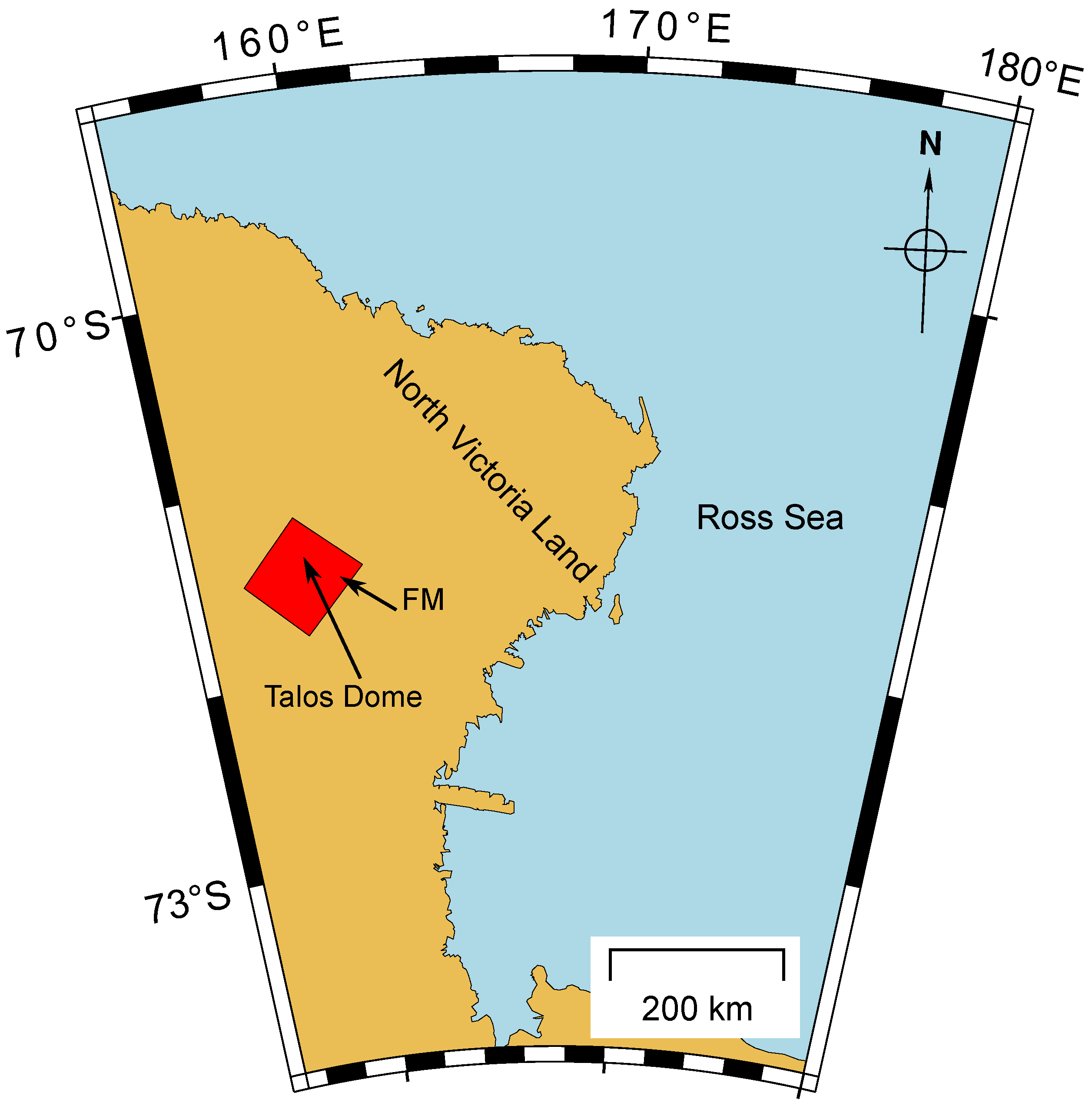
Figure 2.
Talos Dome region SAR magnitude image geocoded using the REMA DEM and the GPS network positioning [8].
Figure 2.
Talos Dome region SAR magnitude image geocoded using the REMA DEM and the GPS network positioning [8].
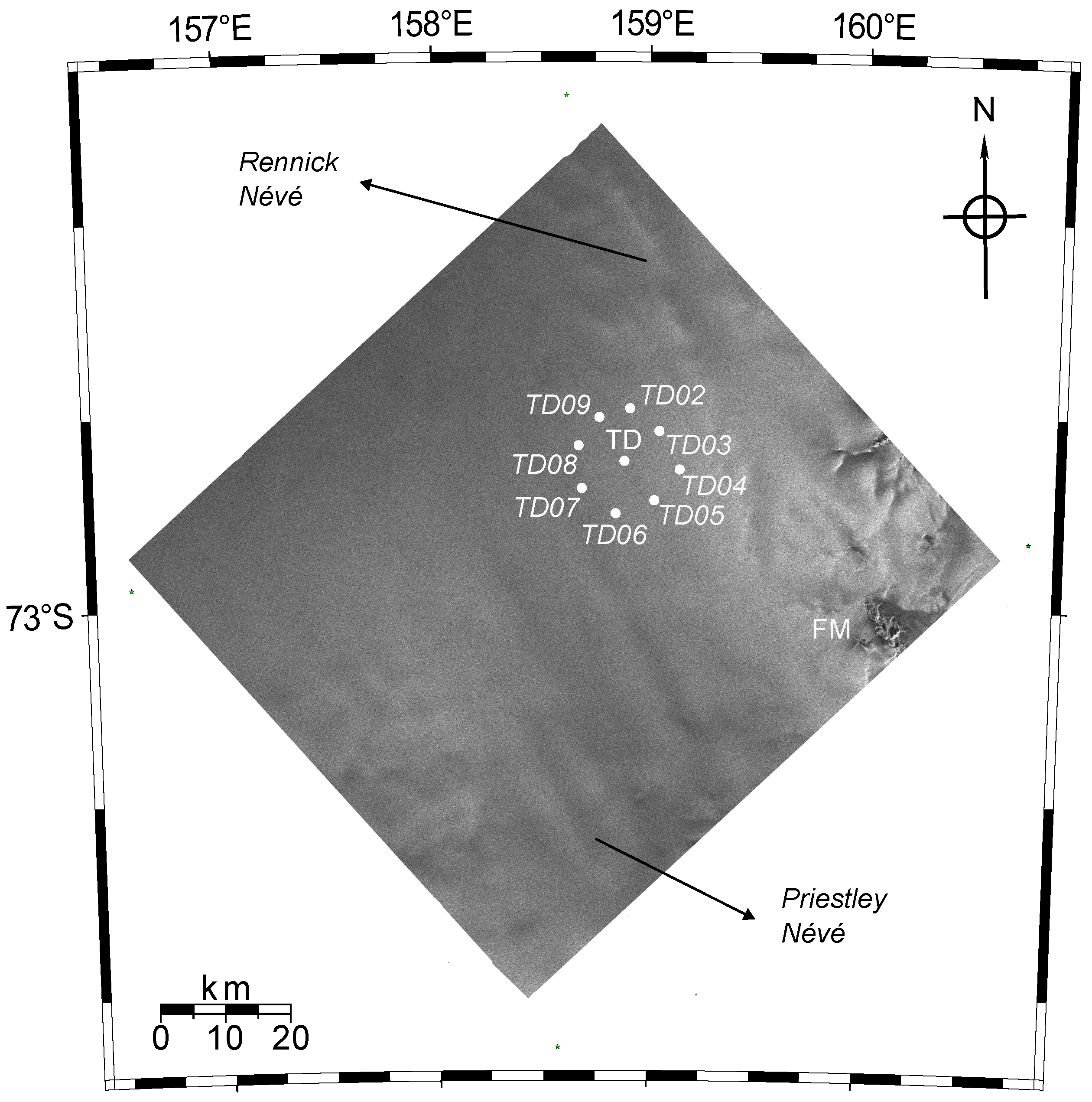
Figure 3.
(a) is the topography interferogram after phase scaling, (b) motion interferogram after phase scaling erasing the topographic component. The two interferograms are in the satellite line of sight.
Figure 3.
(a) is the topography interferogram after phase scaling, (b) motion interferogram after phase scaling erasing the topographic component. The two interferograms are in the satellite line of sight.
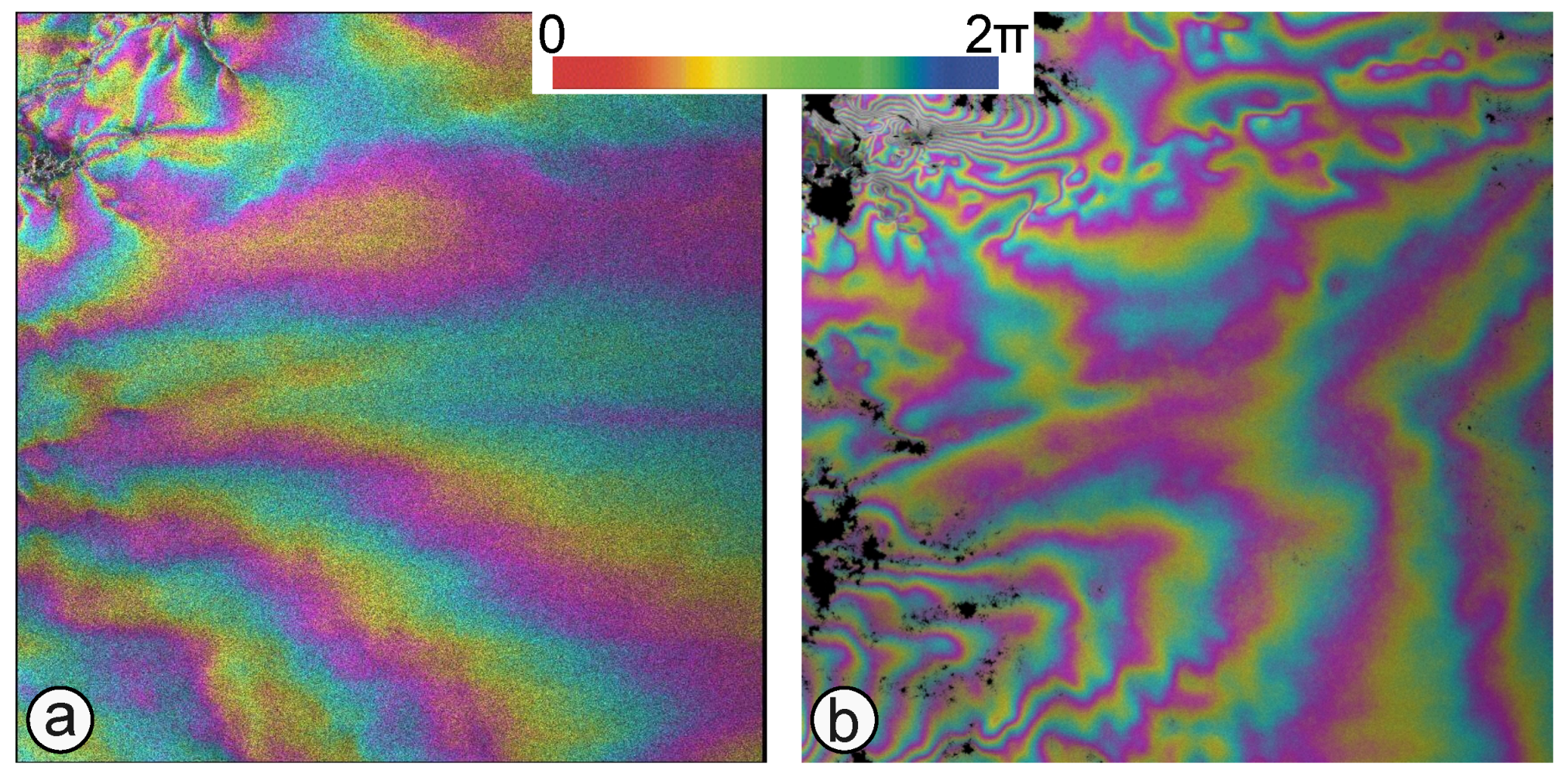
Figure 4.
Regional interferometric DEM of the Talos Dome region with TD and FM locations.
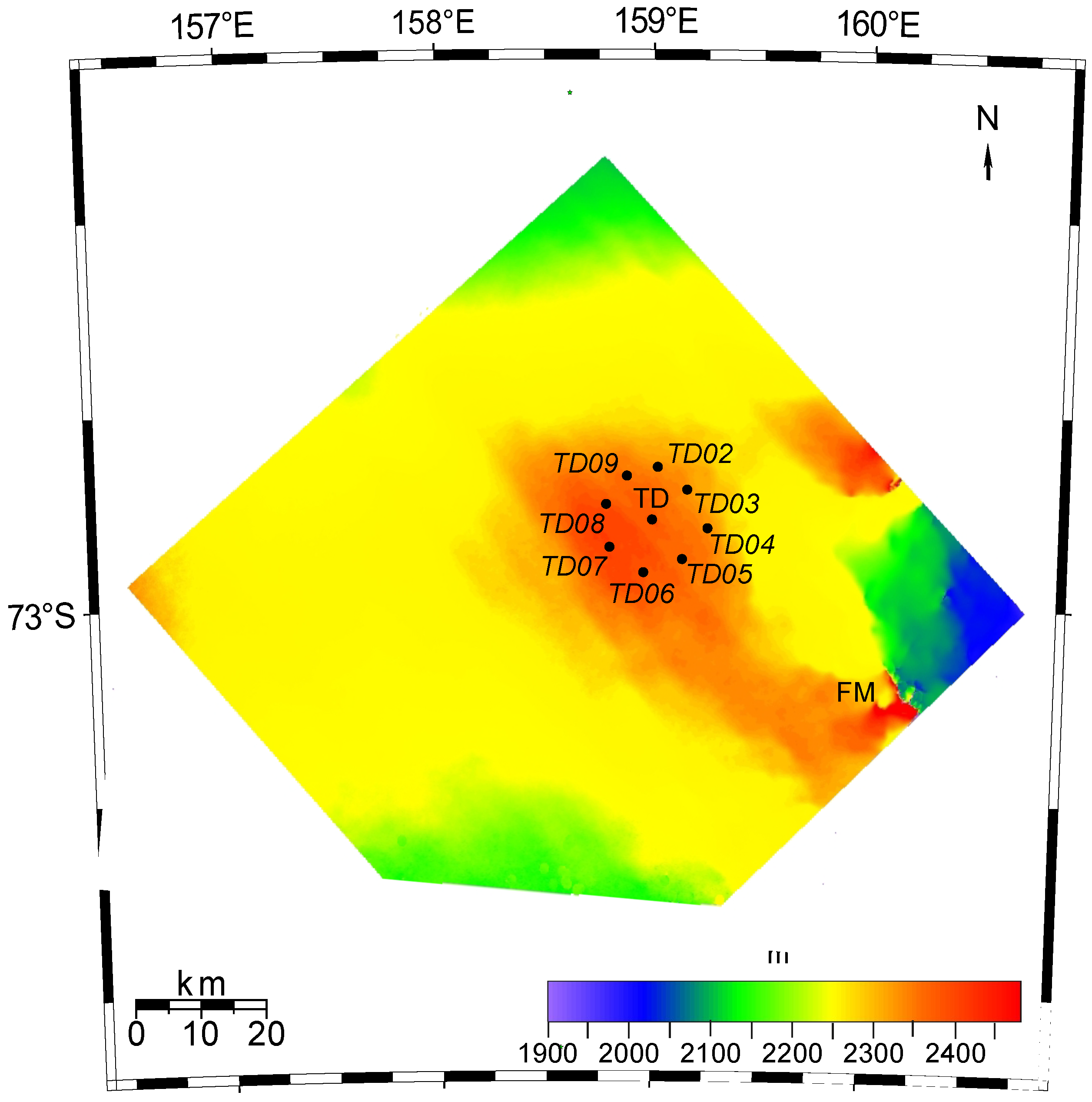
Figure 5.
Differencies between the interferometric and REMA DEMs and the altitude profileTD – GPR23.
Figure 5.
Differencies between the interferometric and REMA DEMs and the altitude profileTD – GPR23.
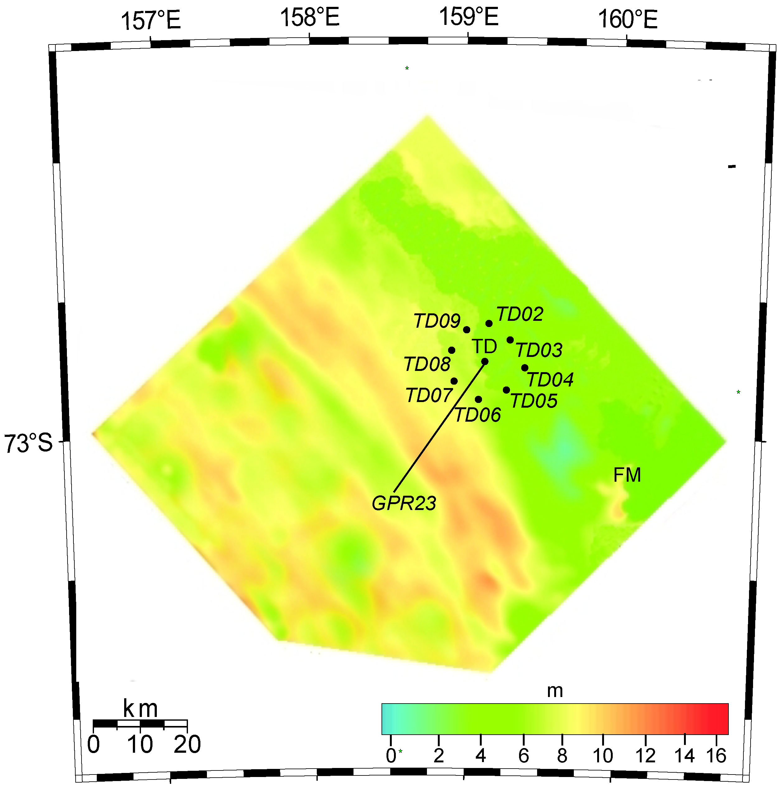
Figure 6.
Altitude profile TD – GPR23 [7].
Figure 6.
Altitude profile TD – GPR23 [7].
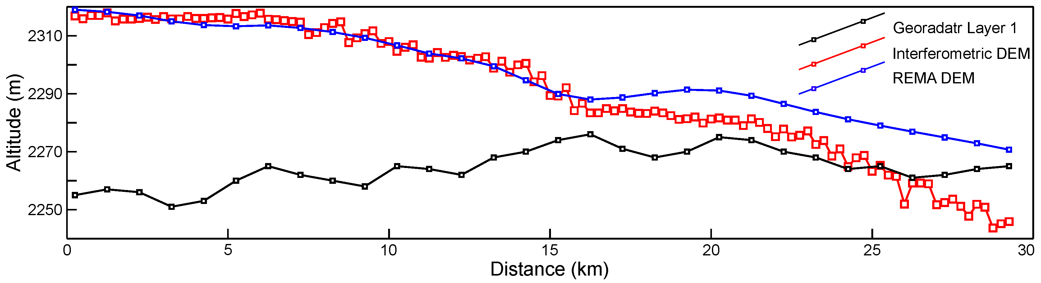
Figure 7.
Talos Dome region SAR 70 days coherence image geocoded using the REMA DEM and the GPS network positioning. White color is indicating a high coherence, black is indicating a low coherence. The yellow dotted line is indicating the layer reflecting the C-radar signal of the ERS satellite.
Figure 7.
Talos Dome region SAR 70 days coherence image geocoded using the REMA DEM and the GPS network positioning. White color is indicating a high coherence, black is indicating a low coherence. The yellow dotted line is indicating the layer reflecting the C-radar signal of the ERS satellite.
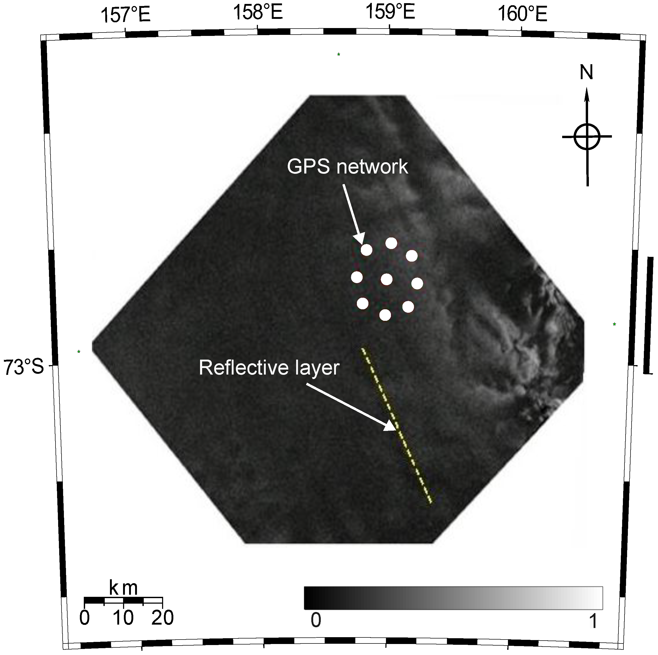
Figure 8.
Rate of change of ice surface elevation from 8 years of altimetric data analysis (after [24]) with superimposed the REMA DEM 50 contour line.
Figure 8.
Rate of change of ice surface elevation from 8 years of altimetric data analysis (after [24]) with superimposed the REMA DEM 50 contour line.
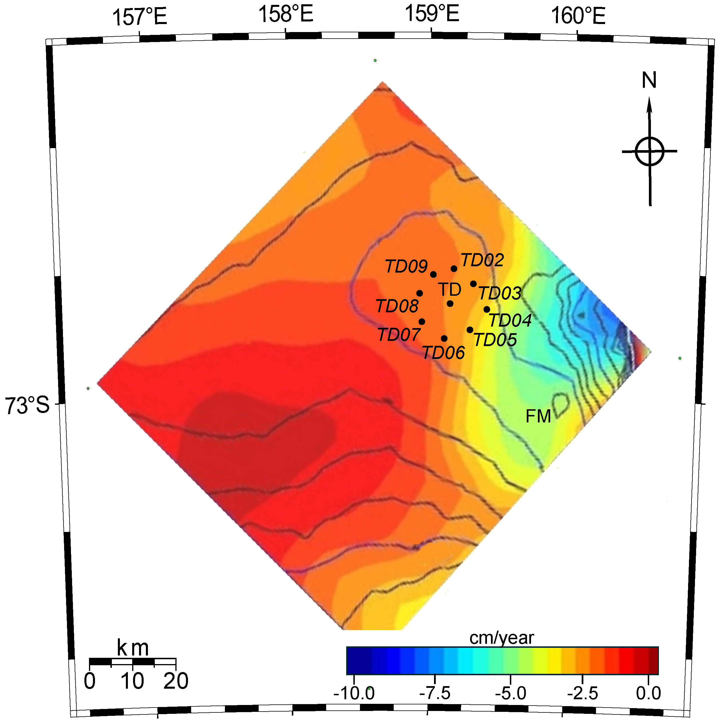
Figure 9.
Ice flow pattern inferred by SAR-interferometry for the same region as shown in Figure 3. Ice movements with an eastward component tend toward the blue color-, movements with a westward component toward the red color spectrum.
Figure 9.
Ice flow pattern inferred by SAR-interferometry for the same region as shown in Figure 3. Ice movements with an eastward component tend toward the blue color-, movements with a westward component toward the red color spectrum.
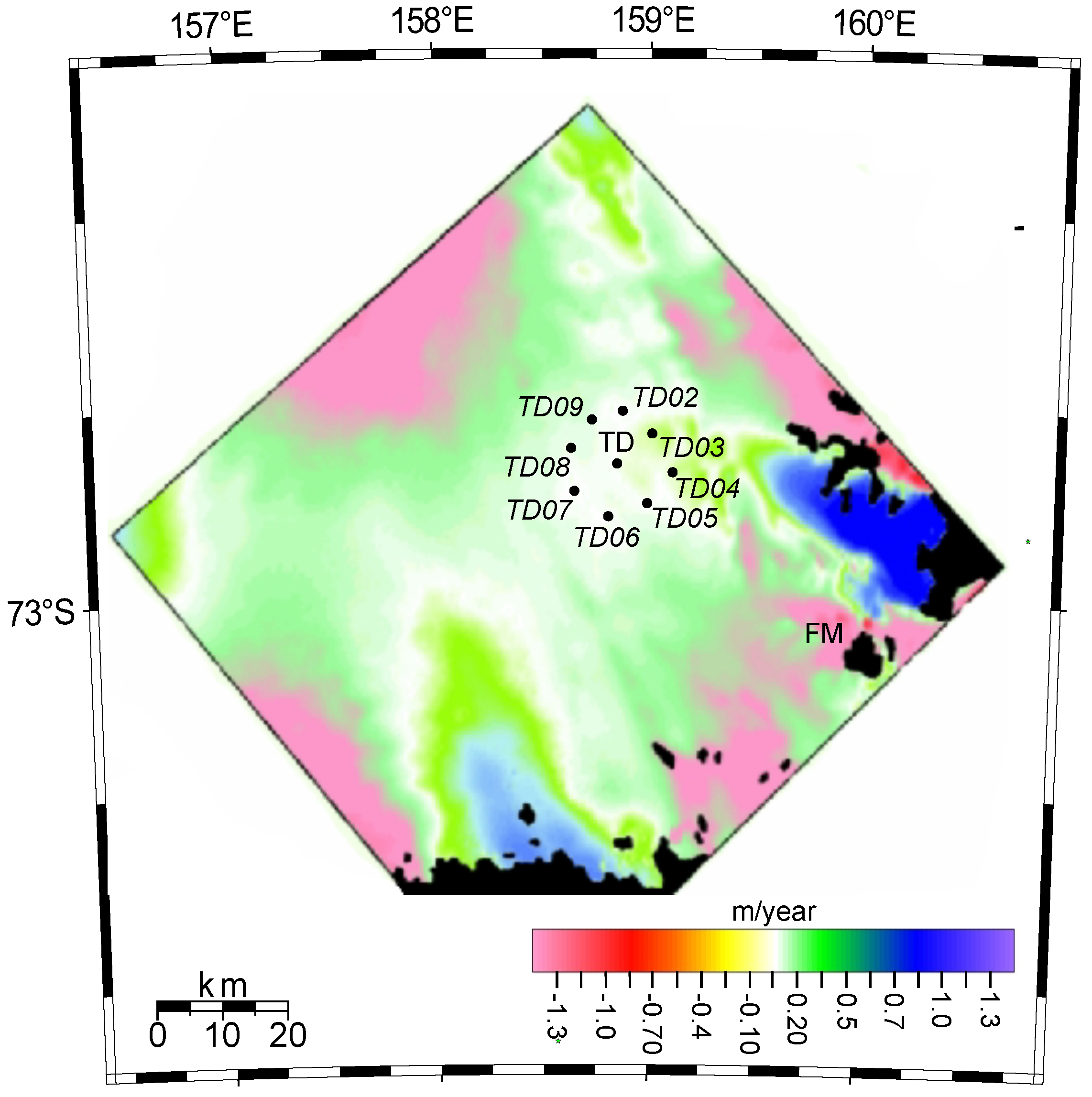
Figure 10.
Frontier mountains radar interferometric velocity field and ice field interpretation of Folco et al. (2002) [9]. Idealized location map of Frontier Mountain in relation to the major meteorite concentration sites. The ”Meteorite Valley“- site is designated as M-MV, the meteorite concentration on the blue ice is designated as M-BI.
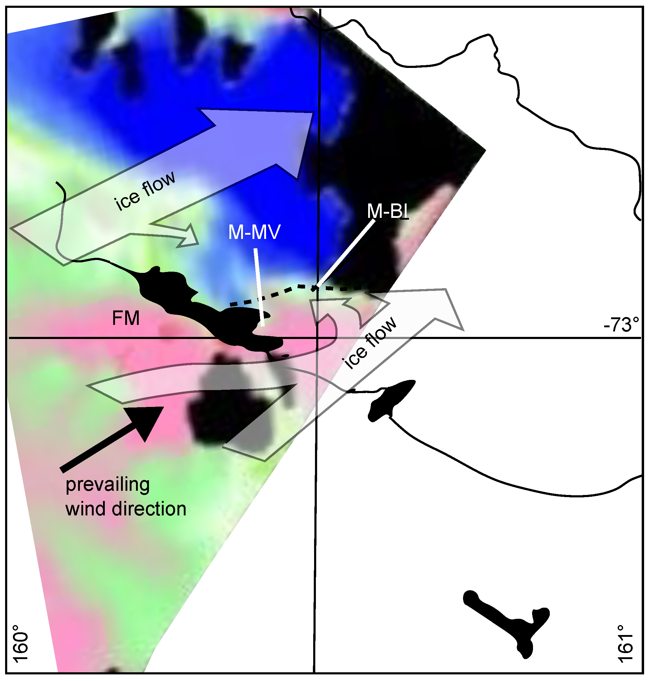

Table 1.
List of synthetic aperture radar scenes used in this study; Bperp = perpendicular component of baseline at mid-swath; Ambiguity = ambiguity height at mid-swath.
Table 1.
List of synthetic aperture radar scenes used in this study; Bperp = perpendicular component of baseline at mid-swath; Ambiguity = ambiguity height at mid-swath.
| Ref. Orbit | Image Num. | Ref. Date | Interf. Orbit | Image Num. | Interf. Date | Elapsed time | (m)a | Ambig. height((m)b) |
|---|---|---|---|---|---|---|---|---|
| E1-23949 | 1 | 1996.01.12 | E2-04276 | 2 | 1996.20.13 | 1 day | ∼132 | ∼68 |
| E1-24951 | 3 | 1996.04.22 | E2-05278 | 4 | 1996.04.23 | 1 day | ∼13 | ∼692 |
Table 2.
Velocity at the TD GPS network points calculated with InSAR and GPS methods.
| TD | 03 | 04 | 05 |
|---|---|---|---|
| INT(m/year) | 0.42±0.14 | 0.35±0.11 | 0.15±0.25 |
| GPS(m/year) | 0.343±13 | 0.336±13 | 0.161±13 |
| Heading | 76° | 82° | 122° |
Disclaimer/Publisher’s Note: The statements, opinions and data contained in all publications are solely those of the individual author(s) and contributor(s) and not of MDPI and/or the editor(s). MDPI and/or the editor(s) disclaim responsibility for any injury to people or property resulting from any ideas, methods, instructions or products referred to in the content. |
© 2024 by the authors. Licensee MDPI, Basel, Switzerland. This article is an open access article distributed under the terms and conditions of the Creative Commons Attribution (CC BY) license (http://creativecommons.org/licenses/by/4.0/).
Copyright: This open access article is published under a Creative Commons CC BY 4.0 license, which permit the free download, distribution, and reuse, provided that the author and preprint are cited in any reuse.


