Attention-Based Deep Learning Models for Cryptocurrency Price Prediction: A Comparative Analysis with Technical Indicators

1. Introduction

The emergence of cryptocurrencies, particularly Bitcoin, has radically transformed the financial landscape by introducing a decentralized, peer-to-peer (P2P) transaction system. First introduced by the pseudonymous Satoshi Nakamoto in 2009, Bitcoin operates without a central authority or intermediary, relying on blockchain technology for secure, transparent, and immutable financial exchanges [1]. The rise of Bitcoin and other cryptocurrencies such as Ethereum and Litecoin has generated significant interest from both financial markets and academic researchers, largely due to their volatile nature and potential for high returns [2]. However, the high volatility and speculative nature of cryptocurrency markets present significant challenges for accurate price prediction [3].

Cryptocurrencies are unique in that their value is driven by a wide range of factors, including macroeconomic variables, technology adoption rates, regulatory developments, and public sentiment [4]. This multifaceted nature of cryptocurrencies complicates the task of price forecasting. Traditional financial models, such as ARIMA and GARCH, have been extensively applied to financial time-series data; however, they are inherently limited by their linear assumptions and inability to account for the non-stationary, highly volatile patterns observed in cryptocurrency prices [5]. As a result, there has been a significant shift toward machine learning and deep learning models, which have demonstrated superior performance in forecasting price movements in volatile markets like cryptocurrencies [6].

Deep learning, a subset of machine learning, has emerged as a powerful tool for cryptocurrency price prediction due to its ability to model complex patterns in large datasets. Among the most prominent deep learning techniques used in financial forecasting are recurrent neural networks (RNNs), particularly Long Short-Term Memory (LSTM) and Gated Recurrent Unit (GRU) models [7]. These models excel at capturing temporal dependencies in sequential data, making them well-suited for predicting time-series data like cryptocurrency prices. LSTMs and GRUs are especially valuable for cryptocurrency markets, where price trends are influenced by both short-term market sentiment and long-term market dynamics [8,9]. Researchers have also explored the use of on-chain data, such as transaction volumes and miner activity, as indicators of future price trends [10]. The predictive power of deep learning models has also been enhanced through the development of hybrid architectures that combine deep learning techniques with other machine learning approaches. For instance, ensemble learning methods, which aggregate the predictions of multiple models, have been shown to reduce bias and variance in cryptocurrency price predictions [11]. These hybrid models, combining financial indicators, sentiment analysis, and technical analysis, have achieved notable success in predicting price movements with higher accuracy than traditional models. Additionally, the application of explainable AI techniques has the potential to enhance the interpretability of these models, offering investors and policymakers greater transparency in the decision-making process [12].

Technical indicators, widely used in traditional financial analysis, offer key insights into market behavior and price momentum. Indicators such as the Relative Strength Index (RSI), Moving Average Convergence Divergence (MACD), and Bollinger Bands provide valuable signals about overbought or oversold conditions in the market and help anticipate price reversals [13]. In this study, we propose a novel deep learning-based cryptocurrency price prediction model that incorporates key technical indicators to enhance prediction accuracy. By leveraging LSTM and GRU architectures, along with these additional market signals, the proposed model seeks to address the limitations of previous studies and provide more reliable and actionable insights for cryptocurrency traders and investors.

2. Related Works

In recent years, predicting cryptocurrency prices has gained significant attention due to the volatile and unpredictable nature of digital asset markets. Traditional models have struggled to capture these complexities, leading to a shift toward deep learning techniques. Ji et al. [14] show that LSTM performs best in regression tasks, while DNN excels in classification. Their findings reveal that classification models are more effective for algorithmic trading, though no single model performs consistently across all scenarios. This highlights the importance of tailoring models to specific prediction goals in dynamic markets.

The introduction of deep learning techniques, particularly LSTM and GRU models, provided a more robust solution for predicting price trends in cryptocurrencies. LSTM and GRU, being recurrent neural networks, excel at capturing long-term dependencies in time-series data, making them well-suited for financial market predictions. Chen et al. [15] finds that statistical models like Logistic Regression perform well with high-dimensional daily data, but machine learning models such as LSTM are more suitable for high-frequency predictions. Their results emphasize the need to match model capabilities to the data’s frequency to prevent overfitting, particularly in markets driven by rapid price changes. The effectiveness of deep learning models also depends on the forecasting horizon. Awoke et al. [16] compare LSTM and GRU models, demonstrating that GRU offers faster convergence and better short-term accuracy, while LSTM is more reliable for capturing long-term patterns. This underscores the importance of selecting models that align with prediction windows to optimize forecast performance.

Following that, Jaquart et al. [17] explore LSTM, GRU, and Gradient Boosting Classifiers, finding that while these models capture short-term dynamics, their predictions align with the efficient market hypothesis. This suggests that despite achieving over 50% accuracy, transaction costs erode potential profits, reflecting the practical challenges of using predictive models in live trading. Also, time-based patterns provide another valuable dimension for prediction. Afterwards, Aljojo et al. [18] achieved 96% accuracy using a Nonlinear Autoregressive Exogenous (NARX) model to analyze how timestamps influence Bitcoin’s open, high, low, and close prices. Their results demonstrate that temporal data plays a pivotal role in identifying subtle market patterns, making such models highly effective for volatile markets. Furthermore, incorporating sentiment data into predictive models adds further depth. Loginova et al. [19] utilize aspect-based sentiment models, extracting sentiment-topic features from platforms like Reddit and CryptoCompare. Their integration of polarity and subjectivity scores not only enhances market trend interpretation but also improves algorithmic trading strategies, showing the growing importance of behavioral data in financial predictions.

The combination of multiple data sources with advanced neural architecture unlocks new predictive capabilities. Kim et al. [20] propose a SAM-LSTM framework that integrates change point detection (CPD) and self-attention mechanisms to process distinct on-chain data groups. Using the PELT algorithm to segment time-series data, their model achieves an MAE of 0.3462 and RMSE of 0.5035, highlighting the potential of combining technical and on-chain data to address market volatility. Also, hybrid architectures offer additional advantages, as demonstrated by Habek et al. [21]. Their CNN-RNN hybrid model achieves 93.77% accuracy by combining CNN for spatial feature extraction with bidirectional LSTM for temporal dependencies. The success of their approach highlights the power of integrating multiple architectures to enhance sentiment analysis and prediction performance. Moving on, Roy et al. [22] compare LSTM, Bi-LSTM, and GRU models, showing that LSTM achieves the lowest RMSE of 409.41, though GRU converges faster. Their study emphasizes the importance of selecting models based on both predictive accuracy and computational efficiency to handle volatile trends effectively.

Avoiding overfitting without compromising accuracy is essential for robust performance. Frohmann et al. [23] address this by integrating sentiment analysis with time-series models, achieving an MAE of 2.67 and RMSE of 3.28. Their work underscores the need for balancing model complexity to maintain high accuracy in rapidly changing markets.

Optimization techniques further enhance predictive models. Tang et al. [24] introduce a PSO-optimized GRU model, fine-tuning parameters such as neuron count, epochs, and batch size. Their approach achieves 10.47% higher accuracy than standard GRU models, demonstrating the value of optimization in managing volatile financial markets and supporting practical risk management strategies. Fang et al. [25] develop an LSTM framework with adaptive retraining, achieving 78% accuracy by processing high-frequency order book data. Their results illustrate the importance of continuous learning and real-time adjustment to sustain model performance in dynamic trading environments.

The integration of complementary architecture offers further potential for improving accuracy. Patel et al. [26] propose a hybrid LSTM-GRU model, trained on a five-year dataset from Yahoo! Finance. Their approach, using MinMax scaling and the Adam optimizer, achieves an RMSE of 409.41, outperforming standalone models and demonstrating the benefits of combining architectures in complex market environments. Subsequently, Arslan et al. [27] combine sentiment analysis with empirical mode decomposition (EMD) and LSTM networks, training parallel models on decomposed price data. Their ensemble model achieves lower RMSE and MAE, illustrating the value of integrating social sentiment with advanced neural networks for cryptocurrency prediction. In addition, effective feature selection enhances predictive performance, as shown by Omole and Enke [28]. Their CNN–LSTM hybrid model incorporates Boruta, genetic algorithms, and LightGBM, achieving 82.44% accuracy. Through backtesting, their long-and-short trading strategy yields an annual return of 6653%, demonstrating the practical value of combining feature selection with deep learning for financial forecasting.

Recent advances in cryptocurrency price prediction have largely focused on integrating deep learning techniques with sentiment analysis, on-chain data, and advanced decomposition methods. These approaches have shown considerable success in capturing the non-linear and volatile dynamics of cryptocurrency markets. Experimental results consistently indicate that hybrid models, which combine multiple data sources—such as social sentiment and high-frequency trading data—deliver the most accurate and actionable insights for traders and investors. However, despite these advancements, existing research often overlooks a comprehensive evaluation of the effectiveness of technical indicators. This gap highlights the need for deeper exploration, which forms the core focus of this study. By systematically analyzing the predictive power of various technical indicators, this research aims to address the shortcomings in current models and provide more robust tools for price forecasting.

3. Research Method

This section details the research methodology and the proposed models in this study, aimed at validating the effectiveness of moving average technical indicators in predicting financial asset trends, specifically in the cryptocurrency market. By leveraging deep learning models, this study assesses how well widely used indicators—Simple Moving Average (SMA), Exponential Moving Average (EMA), Triple Moving Average (TEMA), and Moving Average Convergence Divergence (MACD)—perform in forecasting price movements. These indicators are integrated to capture various aspects of cryptocurrency market trends, providing insights into both short-term and long-term price behavior by smoothing out volatility and identifying underlying patterns in market data.

SMA offers a basic trend indicator by calculating the average price over a defined period, while EMA emphasizes recent prices, making it more responsive to current market conditions. TEMA refines trend detection by reducing the lag associated with EMA, and MACD serves as a key indicator for detecting potential trend reversals by comparing short-term and long-term EMAs. In this study, these technical indicators, combined with OHLCV (open, high, low, close, volume) data, are fed into the proposed Attention-based LSTM and Attention-based GRU models. The models are trained to predict future cryptocurrency price movements (up, down, or neutral) based on these historical inputs. The following sections detail the design of these algorithms and their role in evaluating the predictive power of moving averages in the volatile cryptocurrency market.

3.1. SMA, EMA, TEMA, and MACD

Moving averages are widely used in financial forecasting due to their ability to smooth out price fluctuations and reveal the underlying trend of a market. By averaging past prices, moving averages help to reduce the noise caused by short-term volatility, allowing traders and analysts to better understand the overall direction of an asset’s movement. This makes them particularly useful in identifying potential turning points, such as trend reversals or continuations. In addition, moving averages can adapt to different timeframes, making them versatile tools for both short-term trading strategies and long-term investment decisions, offering clearer signals in volatile markets. 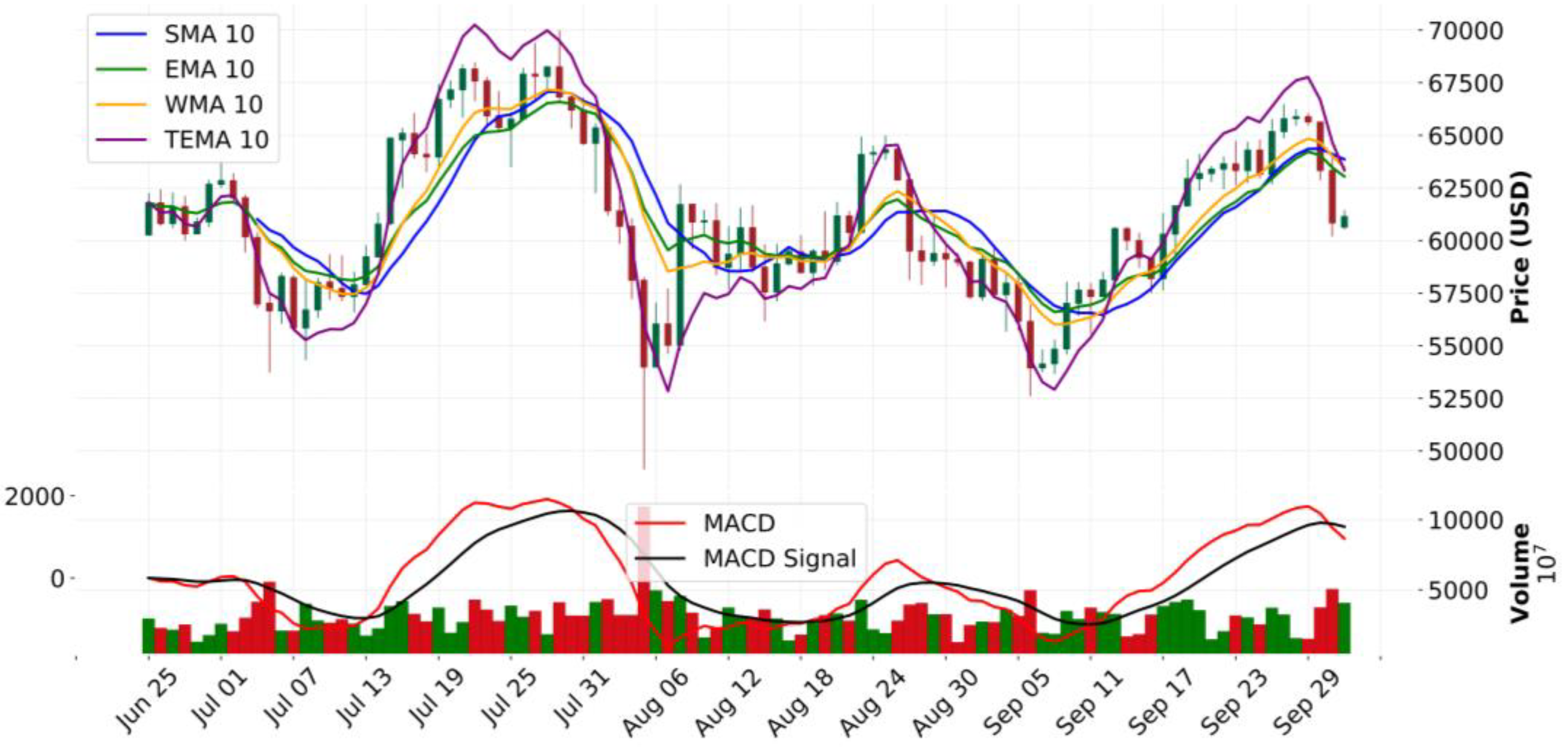Figure 1 shows the Bitcoin price trend in 06~09/2024.

3.1.1. Simple Moving Average (SMA)

Simple Moving Average (SMA) smooths out price data by calculating the average price of an asset over a specified period. It assigns equal weight to all prices within the time window, offering a basic tool for identifying overall market trends. A rising SMA indicates an uptrend, while a declining SMA suggests a downtrend. However, its equal weighting means SMA can lag behind current market conditions, making it slower to respond to recent price shifts. Traders use SMA to gauge general trend direction and potential support or resistance levels. Its calculation is as Equation (1):

$$\mathrm{S}\mathrm{M}{A}_t={\displaystyle \frac{\left(P_t+P_{t-1}+\dots +P_{t-\left(n-1\right)}\right)}{n}}$$

(1)

Where $\mathrm{S}\mathrm{M}{\mathrm{A}}_t$ is the moving average at time t, P_t is the closing price at time t, and n represents the length of the time window. An uptrend and buy signal occur when the price is above the SMA, and the SMA is sloping upwards. A strong buy signal, known as a "Golden Cross," happens when a short-term SMA (e.g., 10-day) crosses above a long-term SMA (e.g., 50-day), indicating upward momentum. Conversely, a downtrend and sell signal occur when the price is below the SMA, and the SMA is sloping downwards. A sell signal, called a "Death Cross," arises when a short-term SMA crosses below a long-term SMA, signaling potential further price declines. Based on this concept, this study normalizes the SMA attributes as follows:

$$S_{SMA,t}=\left\{\begin{array}{c}1,if{P}_t>{\mathrm{S}\mathrm{M}\mathrm{A}}_t\\ -1,if{P}_t<{\mathrm{S}\mathrm{M}\mathrm{A}}_t\\ 0,if{P}_t={\mathrm{S}\mathrm{M}\mathrm{A}}_t\end{array}\right.$$

(2)

3.1.2. Exponential Moving Average (EMA)

Exponential Moving Average (EMA) is a more reactive moving average that gives greater weight to recent price data, making it more sensitive to market changes compared to SMA. This weighting allows the EMA to track the current price trend more closely, making it ideal for short-term trading strategies. The responsiveness of EMA helps traders spot potential reversals more quickly and act on them in volatile markets. Because of this, it’s preferred for markets that change direction rapidly, such as cryptocurrency. Its calculation is as follows:

$$\mathrm{E}\mathrm{M}{\mathrm{A}}_{\mathrm{t}} = \alpha \times P_t + \left(1 - \mathsf{\alpha }\right)\times \mathrm{E}\mathrm{M}{\mathrm{A}}_{\mathrm{t}-1}$$

(3)

Where the smoothing factor $\alpha =2/\left(n+1\right)$. An uptrend and buy signal are indicated when the price is above the EMA, particularly if the EMA is sloping upwards. A buy signal occurs when a short-term EMA (e.g., 12-day) crosses above a long-term EMA (e.g., 26-day), suggesting upward momentum and a likely price increase. Conversely, a downtrend and sell signal are indicated when the price is below the EMA and the EMA is sloping downwards. A sell signal is triggered when the short-term EMA crosses below the long-term EMA, signaling growing downward momentum and the potential for further price declines. Based on this, this study normalizes the EMA attributes as follows:

$$S_{EMA,t}=\left\{\begin{array}{c}1,if{P}_t>{\mathrm{E}\mathrm{M}\mathrm{A}}_t\\ -1,if{P}_t<{\mathrm{E}\mathrm{M}\mathrm{A}}_t\\ 0,if{P}_t={\mathrm{E}\mathrm{M}\mathrm{A}}_t\end{array}\right.$$

(4)

3.1.3. Triple Exponential Moving Average (TEMA)

Triple Exponential Moving Average (TEMA) is designed to reduce the lag associated with regular moving averages by applying three layers of exponential smoothing. TEMA responds faster to price changes, making it useful in volatile markets where traders need timely signals. By applying multiple EMAs, TEMA helps identify significant price trends with greater accuracy, reducing the delay often experienced in other moving averages. It’s particularly favored when quick adjustments to market shifts are necessary. Its calculation is as follows:

$$\mathrm{T}\mathrm{E}\mathrm{M}{\mathrm{A}}_t=3\times \mathrm{E}\mathrm{M}{\mathrm{A}}_t-3\times \mathrm{E}\mathrm{M}\mathrm{A}\left(\mathrm{E}\mathrm{M}{\mathrm{A}}_t\right)+\mathrm{E}\mathrm{M}\mathrm{A}\left(\mathrm{E}\mathrm{M}\mathrm{A}\left(\mathrm{E}\mathrm{M}{\mathrm{A}}_t\right)\right)$$

(5)

An uptrend and buy signal occur when the price crosses above the TEMA, and the TEMA starts sloping upwards, indicating an uptrend with reduced noise compared to traditional moving averages. This crossover is viewed as a buy signal, suggesting that the price may continue to rise steadily. Conversely, a downtrend and sell signal are indicated when the price crosses below the TEMA and the TEMA begins sloping downwards. This crossover serves as a sell signal, signaling that the price may continue to fall with less interference from small fluctuations. Based on this, this study normalizes the TEMA attributes as follows:

$$S_{TEMA,t}=\left\{\begin{array}{c}1,if{P}_t>{\mathrm{T}\mathrm{E}\mathrm{M}\mathrm{A}}_t\\ -1,if{P}_t<{\mathrm{T}\mathrm{E}\mathrm{M}\mathrm{A}}_t\\ 0,if{P}_t={\mathrm{T}\mathrm{E}\mathrm{M}\mathrm{A}}_t\end{array}\right.$$

(6)

3.1.4. Moving Average Convergence Divergence (MACD)

Moving Average Convergence Divergence (MACD) compares two EMAs to measure market momentum. It is used to detect shifts in the trend, where the difference between short-term and long-term EMAs indicates potential buying or selling opportunities. A positive MACD shows upward momentum, while a negative value suggests downward momentum. The MACD line crossing above or below a signal line provides clear entry and exit points for traders looking to capitalize on market movements. Its calculation is as follows:

$$\mathrm{M}\mathrm{A}\mathrm{C}{\mathrm{D}}_t=\mathrm{E}\mathrm{M}{\mathrm{A}}_{12}\left(P_t\right)-\mathrm{E}\mathrm{M}{\mathrm{A}}_{26}\left(P_t\right)$$

(7)

Where $\mathrm{E}\mathrm{M}{\mathrm{A}}_{12}\left(P_t\right)$ and $\mathrm{E}\mathrm{M}{\mathrm{A}}_{26}\left(P_t\right)$ are 12-day and 26-day exponential moving average of the closing price, respectively. An uptrend and buy signal are reflected when the MACD line is above the zero line (positive), indicating upward momentum. A buy signal is generated when the MACD line crosses above the signal line (bullish crossover), suggesting that the trend is gaining upward strength, and the price is likely to continue rising. Conversely, a downtrend and sell signal are indicated when the MACD line is below the zero line (negative), showing downward momentum. A sell signal occurs when the MACD line crosses below the signal line (bearish crossover), indicating the trend is weakening, and the price may continue to fall. Based on this, this study normalizes the MACD attributes as follows:

$${\mathrm{M}\mathrm{A}\mathrm{C}\mathrm{D}}_{Signa{l}_t}=\mathrm{E}\mathrm{M}{\mathrm{A}}_9\left(\mathrm{M}\mathrm{A}\mathrm{C}{\mathrm{D}}_t\right)$$

(8)

$$S_{MACD,t}=\left\{\begin{array}{c}1,if{\mathrm{M}\mathrm{A}\mathrm{C}\mathrm{D}}_t>{\mathrm{M}\mathrm{A}\mathrm{C}\mathrm{D}}_{Signa{l}_t}\\ -1,if{\mathrm{M}\mathrm{A}\mathrm{C}\mathrm{D}}_t<{\mathrm{M}\mathrm{A}\mathrm{C}\mathrm{D}}_{Signa{l}_t}\\ 0,ifMACD={\mathrm{M}\mathrm{A}\mathrm{C}\mathrm{D}}_{Signa{l}_t}\end{array}\right.$$

(9)

3.2. The Proposed Attention-Based Deep Models

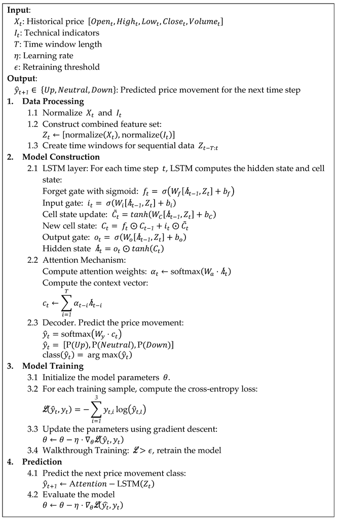
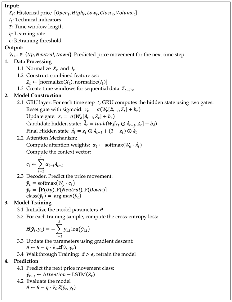
The following sections present two deep learning algorithms designed to predict cryptocurrency price movements using historical OHLCV data and technical indicators. These algorithms aim to capture both long-term and short-term market dynamics by integrating advanced attention mechanisms, which allow the models to focus on the most relevant time steps. Algorithm 1 employs an Attention-based LSTM architecture, leveraging LSTM’s strength in modeling sequential dependencies, while Algorithm 2 uses an Attention-based GRU architecture, which offers computational efficiency and faster training while maintaining predictive power. Both algorithms utilize technical indicators as input enhancements to improve the model’s ability to classify price movement into three categories: uptrend, downtrend, or neutral, with a final classification made using the Softmax function.

In the proposed algorithms, $h_t$ is the hidden state at time t, ${\alpha }_t$ is the attention weight at time t, $c_t$ is the context vector computed by the attention mechanism, $\sigma$ is the sigmoid function, $⨀$ represents the Hadamard product, Tanh refers to the hyperbolic tangent, and ${\widehat{y}}_t$ and $\mathcal{L}$ represent the predicted price movement class and cross-entropy loss function, respectively. Both Algorithm 1 (Attention-based LSTM) and Algorithm 2 (Attention-based GRU) operate within a deep learning framework optimized for sequence modeling, with slight architectural differences influencing their behavior. Each model processes sequential data by transforming input features through several hidden layers, leveraging recurrent connections to capture complex relationships in time series data. The attention mechanism enhances performance by redistributing focus across varying time steps, helping the models mitigate issues related to vanishing gradients.

Algorithm 1 employs LSTM cells to address challenges in retaining long-term dependencies. The architecture manages internal states using carefully tuned input, forget, and output gates, regulating the information flow between time steps. Algorithm 2 incorporates GRU cells, which simplify the recurrent structure without sacrificing learning capacity. The GRU’s design combines memory gates, minimizing computational overhead while still preserving essential temporal information. This lightweight architecture not only enables faster convergence but also makes it well-suited for dynamic market conditions where rapid adaptation is crucial.

4. Experimental Results

4.1 Experimental Setup

The experiments were conducted on an ASUS system equipped with an Intel® Core™ i9 processor, 32GB of RAM, and an NVIDIA GeForce RTX 3060 Super graphics card, running on Windows 10 Enterprise. The dataset comprised 2,192 Bitcoin transaction records from September 30, 2018, to September 30, 2024, sourced from Yahoo Finance. It included daily high, low, open, and close prices, along with trading volume, offering a detailed representation of Bitcoin's price movements and market behavior during this period. The model incorporated four technical indicators - SMA, EMA, TEMA, and MACD, each calculated daily and normalized using their respective moving averages. This normalization was crucial in ensuring the model processed the indicators effectively, smoothing out volatility and maintaining consistency across the data. The window size was set to 10, and the training was conducted over 200 epochs, with a batch size of 32. The dataset was split into 80% for training, 20% for validation, and all data were used for backtesting, ensuring a balanced approach to model evaluation. The system's computational power was leveraged to handle the deep learning model's complexity, ensuring efficient processing and training over the specified period.

4.2 Experimental Results

In this study, we evaluated the performance of classification models using key metrics to ensure a detailed understanding of their effectiveness. The metrics used include Accuracy, Precision, Recall, and F1 Measure. All measures are calculated as follows:

$$Accuracy={\displaystyle \frac{TP+TN}{TP+TN+FP+FN}}$$

(10)

$$Precision={\displaystyle \frac{TP}{TP+FP}}$$

(11)

$$Recall={\displaystyle \frac{TP}{TP+FN}}$$

(12)

$$F1=2\times {\displaystyle \frac{Precision\times Recall}{Precision+Recall}}$$

(13)

Where True Positives (TP) are positive cases that were correctly classified, while True Negatives (TN) are negative cases that were correctly classified. False Positives (FP) refer to negative cases that were incorrectly classified as positive, and False Negatives (FN) are positive cases incorrectly classified as negative. In this study, Recall, Precision, F1 Measure, and Accuracy are key evaluation metrics used to assess the performance of the model in forecasting price movements. Recall measures the model’s ability to correctly predict upward trends when they actually occur, ensuring that most trading opportunities are captured, and potential profits are not missed. Precision focuses on the accuracy of the model’s upward trend predictions, helping to minimize false signals and reduce unnecessary trading risks. To balance Precision and Recall, this study employs the F1 Measure as a composite metric, using its harmonic means to provide a more reliable performance evaluation, especially when dealing with imbalanced data. Finally, Accuracy quantifies the proportion of correct predictions across all outcomes, offering an overall measure of the model's effectiveness in both upward and downward trend forecasting.

4.2.1. Results of Attention-based LSTM Model

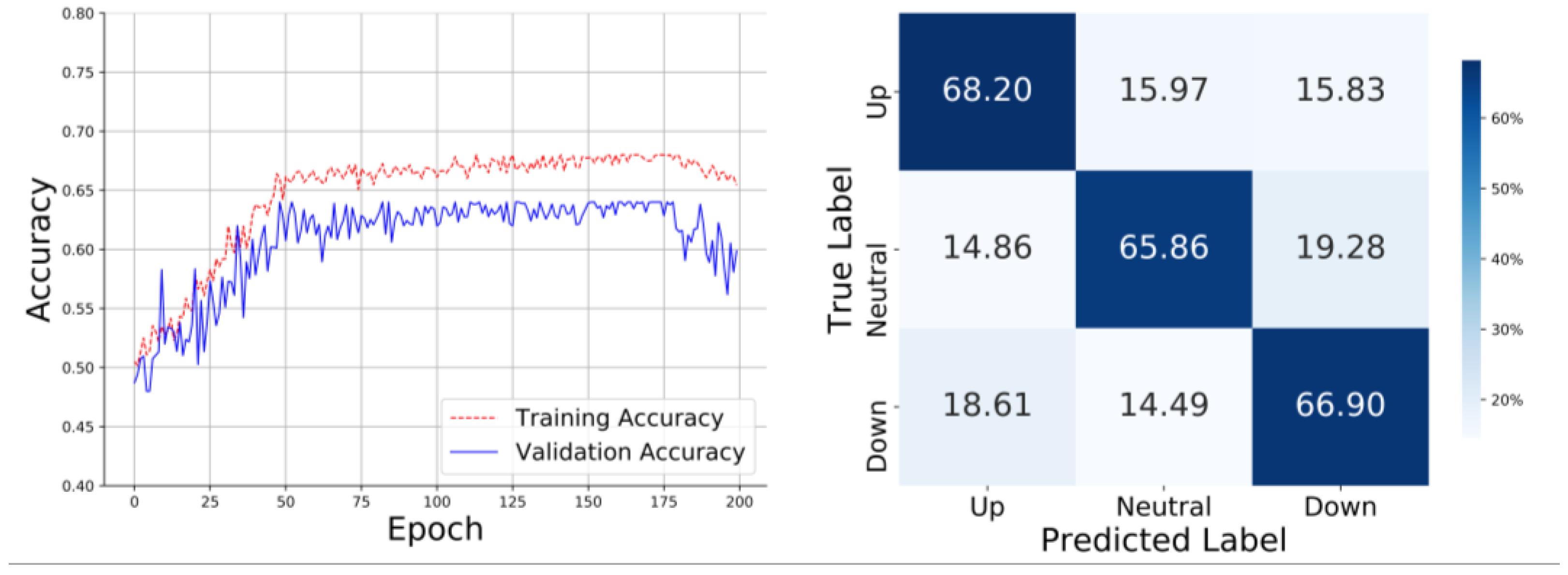
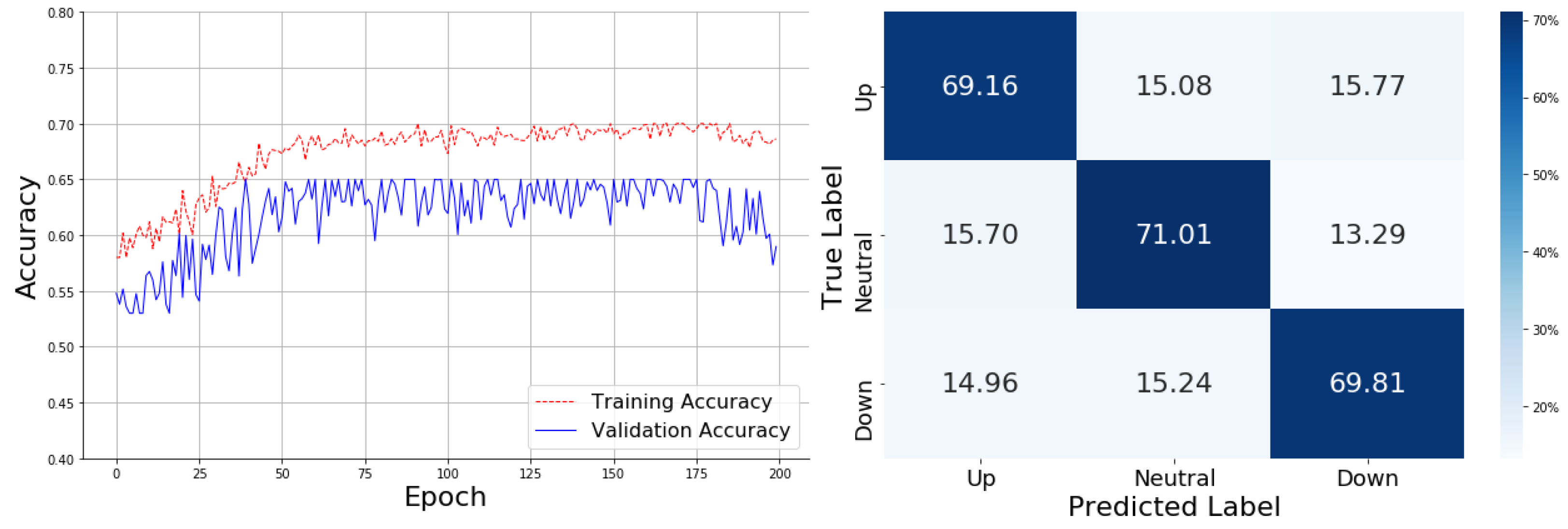
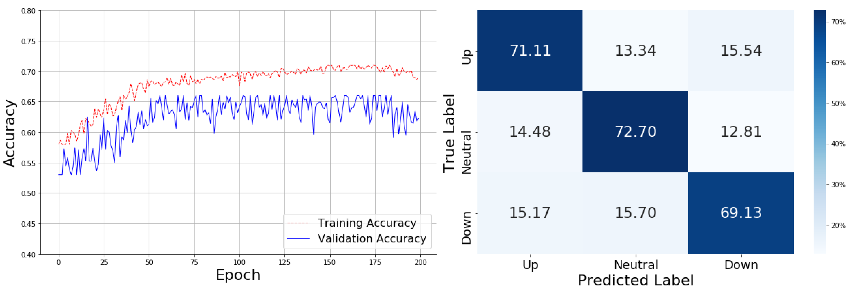
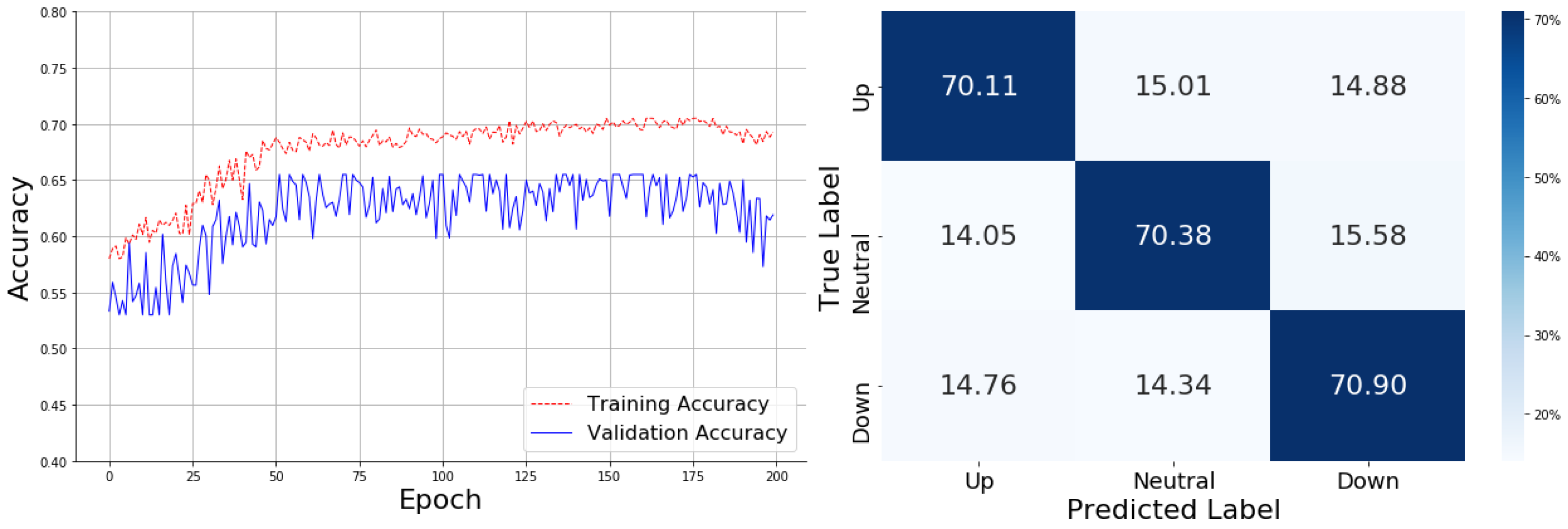
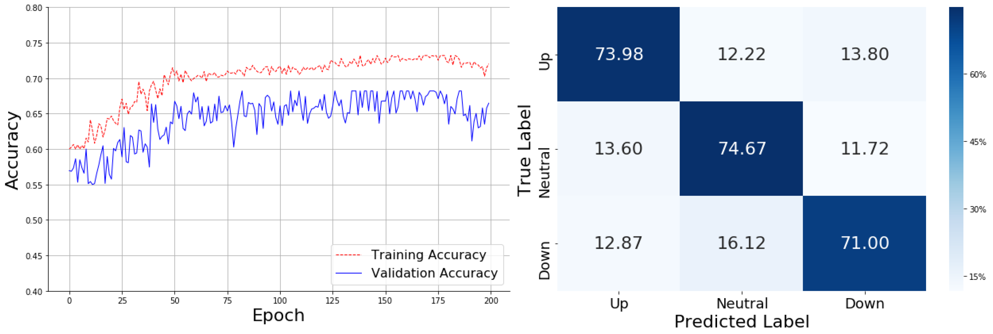
The analysis below presents the experimental findings for the Attention-based LSTM model. Figures 2~6 demonstrate the model's performance across various configurations: without any technical indicators, and with SMA, EMA, TEMA, and MACD included respectively. Each figure showcases both the training and validation accuracy trends along with their corresponding confusion matrices. These results provide a detailed view of the model’s classification effectiveness across the "Up," "Neutral," and "Down" categories, highlighting the impact of each technical indicator on the model’s accuracy and generalization.

In the absence of technical indicators, the training curve shows a steady increase from around 0.50 to a peak of approximately 0.65 over 200 epochs. However, fluctuations towards the end suggest potential overfitting. The confusion matrix shows that the model correctly classifies 68.20% of the "Up" cases, 65.86% of the "Neutral" cases, and 66.90% of the "Down" cases. However, there are significant misclassifications, such as 15.97% of "Up" cases being misclassified as "Neutral," and 18.61% of "Down" cases being misclassified as "Up." This highlights that the model struggles to differentiate between the "Up" and "Down" categories, often confusing the two, as shown in Figure 2.

With the SMA technical indicator, the training curve improves quickly from 0.50 to nearly 0.70, stabilizing towards the end of the 200 epochs. SMA significantly helps the model converge faster. The confusion matrix shows the model achieving 69.16% accuracy for the "Up" category, 71.01% for "Neutral," and 69.81% for "Down." Despite this improvement, there are notable misclassifications, such as 15.70% of "Neutral" cases being classified as "Up" and 14.96% of "Down" cases misclassified as "Up." The tendency to mistake "Down" for "Up" suggests that SMA slightly improves general accuracy but still faces challenges in distinguishing between "Up" and "Down". As shown in Figure 3.

In Figure 4, the training curve under the EMA indicator rises from 0.50 to 0.70, demonstrating faster convergence and increased stability over time compared to no indicators. In the confusion matrix, the model achieves an accuracy of 71.11% for "Up," 72.70% for "Neutral," and 69.13% for "Down." However, the confusion matrix reveals that 14.48% of "Neutral" cases were misclassified as "Up," and 15.17% of "Down" cases were misclassified as "Neutral." This suggests that while the overall accuracy improves, the model struggles to differentiate between "Neutral" and "Down" categories, leading to higher confusion between these classes.

The TEMA indicator shows the training curve rising rapidly to 0.65 within the first 50 epochs, eventually stabilizing at around 0.70. The confusion matrix reveals that the model predicts 70.11% of "Up" cases correctly, 70.38% of "Neutral" cases, and 70.90% of "Down" cases. However, significant misclassifications remain, such as 15.01% of "Up" cases being predicted as "Neutral" and 14.76% of "Down" cases being misclassified as "Up." This indicates that the model struggles to clearly separate the "Up" and "Neutral" categories, suggesting that TEMA improves the stability of the training curve but still leads to confusion among similar classes, as shown in Figure 5.

In Figure 6, MACD yields the most stable training curve, rapidly rising to around 0.70 and peaking at approximately 0.73, with minimal fluctuations. The confusion matrix reflects high accuracy across categories: 74.27% for "Up," 72.85% for "Neutral," and 73.32% for "Down." Despite this, "Down" was misclassified as "Up" (13.48%), and "Neutral" was mistaken for "Down" (13.21%). These misclassifications suggest that even with MACD, the model occasionally struggles to distinguish between "Down" and "Neutral" labels.

4.2.2. Results of Attention-based GRU Model

The following analysis presents the experimental results of the Attention-based GRU model. Figures 7~11 illustrate the performance of the model under different settings: without technical indicators, and with SMA, EMA, TEMA, and MACD applied respectively. These figures detail the training and validation accuracy curves alongside their corresponding confusion matrices, providing insights into the model’s classification ability across the "Up," "Neutral," and "Down" categories for each technical indicator.

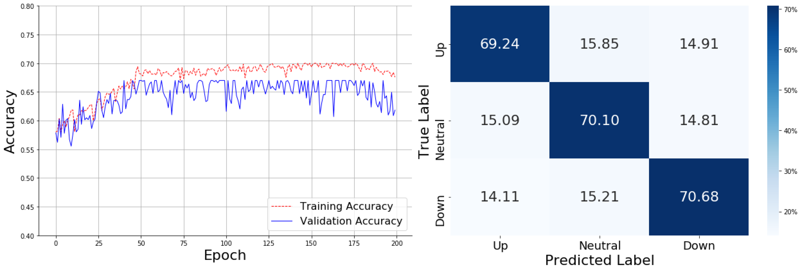
The model without technical indicators, as represented in Figure 7, shows training accuracy rising steadily to 0.65 within the first 50 epochs, eventually stabilizing around 0.69. The validation accuracy, however, fluctuates more noticeably, peaking around 0.66 and showing a wider gap compared to the training accuracy, indicating some overfitting. The confusion matrix reveals that the model correctly predicts 69.24% of "Up" cases, 70.10% of "Neutral" cases, and 70.68% of "Down" cases. Despite these results, the model still misclassifies 15.85% of "Up" cases as "Neutral" and 14.11% of "Down" cases as "Up." This misclassification between the "Up" and "Down" categories suggests that without technical indicators, the model struggles to accurately differentiate these similar market movements, indicating a potential limitation in the model's ability to capture finer distinctions between upward and downward trends.

With the addition of SMA, as shown in Figure 8, the training curve initially rises quickly to approximately 0.65 within the first 50 epochs. After this initial increase, the training accuracy gradually stabilizes around 0.69, similar to the previous model without technical indicators. The validation curve fluctuates more significantly, peaking at around 0.65, and continues to display instability compared to the training accuracy. The confusion matrix for the SMA-enhanced model shows that 69.21% of "Up" cases, 72.40% of "Neutral" cases, and 68.41% of "Down" cases are predicted correctly. Despite this improvement in the "Neutral" class prediction, misclassifications still exist, such as 16.36% of "Down" cases being classified as "Up" and 15.53% of "Neutral" cases misclassified as "Down." These misclassifications suggest that while the SMA indicator helps improve the model’s general performance, especially for the "Neutral" category, the model still struggles to cleanly separate "Down" and "Up" cases. This indicates that the model may benefit from more refined feature extraction to reduce the overlap in predictions for these market trends.

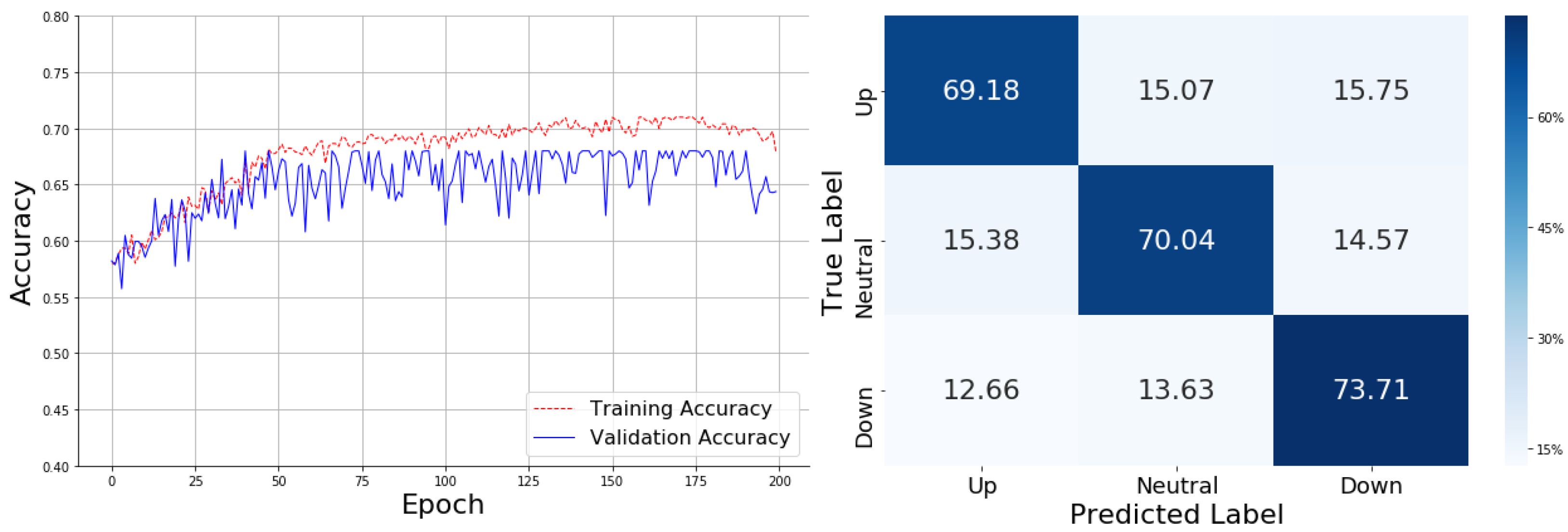
Incorporating the EMA, as represented in Figure 9, the training curve shows an initial sharp rise to approximately 0.65 within the first 50 epochs, followed by a gradual increase that stabilizes around 0.69. The validation curve, on the other hand, exhibits significant fluctuations, peaking at around 0.65 but failing to achieve a stable upward trend, indicating some challenges in the model’s generalization.

The confusion matrix for the EMA-enhanced model reveals that 69.18% of "Up" cases, 70.04% of "Neutral" cases, and 73.71% of "Down" cases are predicted correctly. However, misclassifications persist, with 12.66% of "Down" cases being classified as "Up" and 15.38% of "Neutral" cases misclassified as "Up." This suggests that the model, while performing well in distinguishing "Down" cases, still encounters difficulties in clearly differentiating between "Up" and "Neutral" categories. These classification errors indicate that the EMA indicator may have provided some benefit for identifying downward trends, but further refinement is needed to improve the model’s ability to distinguish between market trends, particularly in the "Up" and "Neutral" categories.

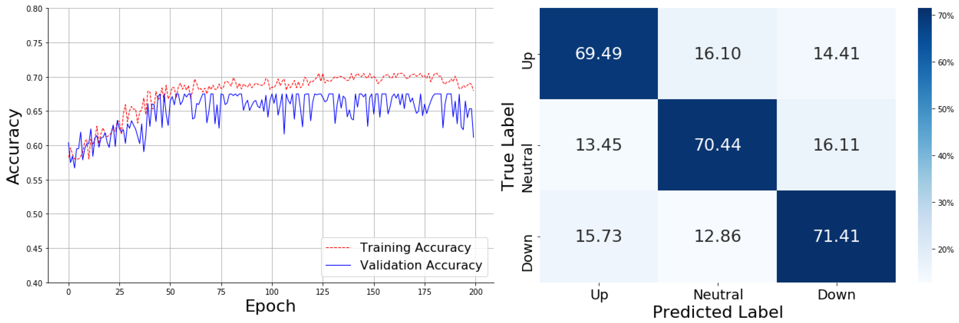
For the TEMA, as shown in Figure 10, the training curve exhibits a steady climb, reaching approximately 0.65 within the first 50 epochs and eventually stabilizing at around 0.70. The validation curve shows more volatility, with notable fluctuations around 0.65, indicating a less stable generalization performance compared to the training accuracy. The model shows a clear improvement in learning, but the gap between the training and validation accuracy implies potential overfitting, as the validation curve remains unstable throughout the epochs.

The confusion matrix reveals that the TEMA-enhanced model correctly predicts 69.49% of "Up" cases, 70.44% of "Neutral" cases, and 71.41% of "Down" cases. Despite these relatively high accuracy rates, there are still some notable misclassifications, particularly in "Down" cases, where 15.73% were classified as "Up." Additionally, 16.10% of "Neutral" cases were misclassified as "Up." This suggests that while TEMA has improved the model's ability to predict market trends, especially for "Neutral" and "Down" categories, it still struggles with clear separation between similar classes, such as "Up" and "Neutral," leading to classification errors.

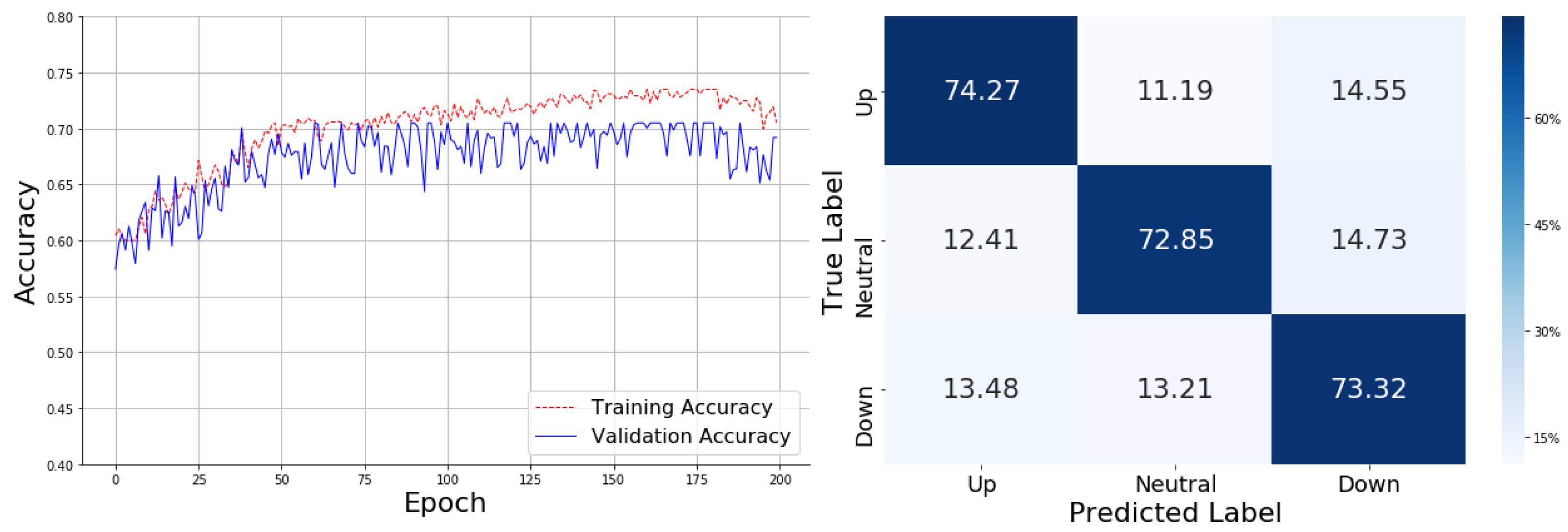
In Figure 11, the MACD demonstrates a training accuracy curve that increases rapidly within the first 50 epochs, reaching approximately 0.68 and stabilizing around 0.74 after 100 epochs. The validation accuracy fluctuates between 0.67 and 0.70, closely aligning with the training accuracy, which indicates improved generalization. The reduced gap between the training and validation curves suggests a balanced model with minimal overfitting, offering greater stability compared to the previous models.

The confusion matrix shows that the MACD-enhanced model achieves the highest average performance, correctly classifying 74.27% of "Up" cases, 72.85% of "Neutral" cases, and 73.32% of "Down" cases. While some misclassifications persist, particularly between "Up" and "Down" signals—where 14.55% of "Up" cases were predicted as "Down" and 13.48% of "Down" cases were predicted as "Up" - this model provides the best overall results in terms of accuracy. The consistent performance across categories and minimal fluctuation makes the MACD-based model the top performer among all tested technical indicators.

4.2.3. Comprehensive Performance Analysis

Table 1 and Table 2 present the comprehensive performance metrics of the Attention-based LSTM and GRU models across different configurations: without technical indicators, and with SMA, EMA, TEMA, and MACD indicators. This comparison offers insight into how each model performs under various setups and highlights the strengths and challenges associated with the use of these technical indicators. Both models demonstrate improvements in accuracy and other key metrics with the inclusion of technical indicators, especially with MACD. For the Attention-based LSTM, the highest accuracy of 73.84% is achieved with MACD, reflecting its superior classification capability. Similarly, the Attention-based GRU also shows the best performance with MACD, achieving an accuracy of 73.21%. Across the board, the inclusion of technical indicators improves precision, recall, and F1-measure for both models compared to their performance without indicators.

The Attention-based GRU model shows slightly higher recall across the configurations, with GRU_MACD achieving the highest recall at 54.37%. This indicates that the GRU model is marginally better at capturing positive instances across the categories compared to the LSTM, as the highest LSTM recall (54.26%) is also achieved with MACD. However, the differences in recall between the models are relatively small, suggesting both architectures have comparable sensitivity. Precision measures how well the models avoid false positives, and here, Attention-LSTM_MACD outperforms the GRU counterpart with 73.27% precision compared to 68.27% for GRU_MACD. This reflects that the LSTM model demonstrates slightly better precision overall, suggesting it may be better at minimizing incorrect classifications.

In terms of the F1-measure, which balances recall and precision, both models show consistent improvements with technical indicators. The LSTM_MACD achieves the highest F1-measure of 62.35%, followed closely by GRU_MACD at 60.53%. The similarity in F1-measure highlights that both models achieve comparable trade-offs between precision and recall with the MACD indicator. Accuracy trends reveal a key insight: both models achieve higher performance with the MACD indicator, with LSTM_MACD slightly outperforming GRU_MACD (73.84% vs. 73.21%). The GRU model shows more stable performance across the indicators, with smaller fluctuations in accuracy. This stability may reflect the GRU’s ability to handle sequential dependencies effectively, offering consistent results even with simpler indicators like SMA and TEMA.

The experimental results reveal that technical indicators play a crucial role in enhancing the models' predictive capability. Indicators provide meaningful insights into market trends, improving the models' ability to differentiate between "Up," "Neutral," and "Down" movements. This added information helps the models generalize better and reduce overfitting, resulting in more stable predictions. Notably, the inclusion of indicators like MACD offers deeper trend analysis, which refines decision boundaries and minimizes ambiguity across classes. This demonstrates that integrating technical indicators optimizes model performance by aligning predictions more closely with underlying market patterns.

5. Conclusions

The experimental findings show that integrating technical indicators meaningfully enhances the performance of both Attention-based LSTM and GRU models. Across the trials, the MACD indicator consistently provided the best results, achieving an accuracy of 73.21% with the GRU model and 73.84% with the LSTM model. SMA and TEMA also delivered stable performance, each contributing to a slight improvement in prediction precision. Notably, the GRU model showed faster convergence while maintaining an accuracy comparable to the LSTM, offering computational efficiency for real-time trading systems. These results highlight the effectiveness of attention-based architectures with indicator enhancements, underscoring the value of momentum-based indicators in volatile cryptocurrency markets.