Submitted:
24 October 2024
Posted:
25 October 2024
You are already at the latest version
Abstract
Keywords:
1. Introduction
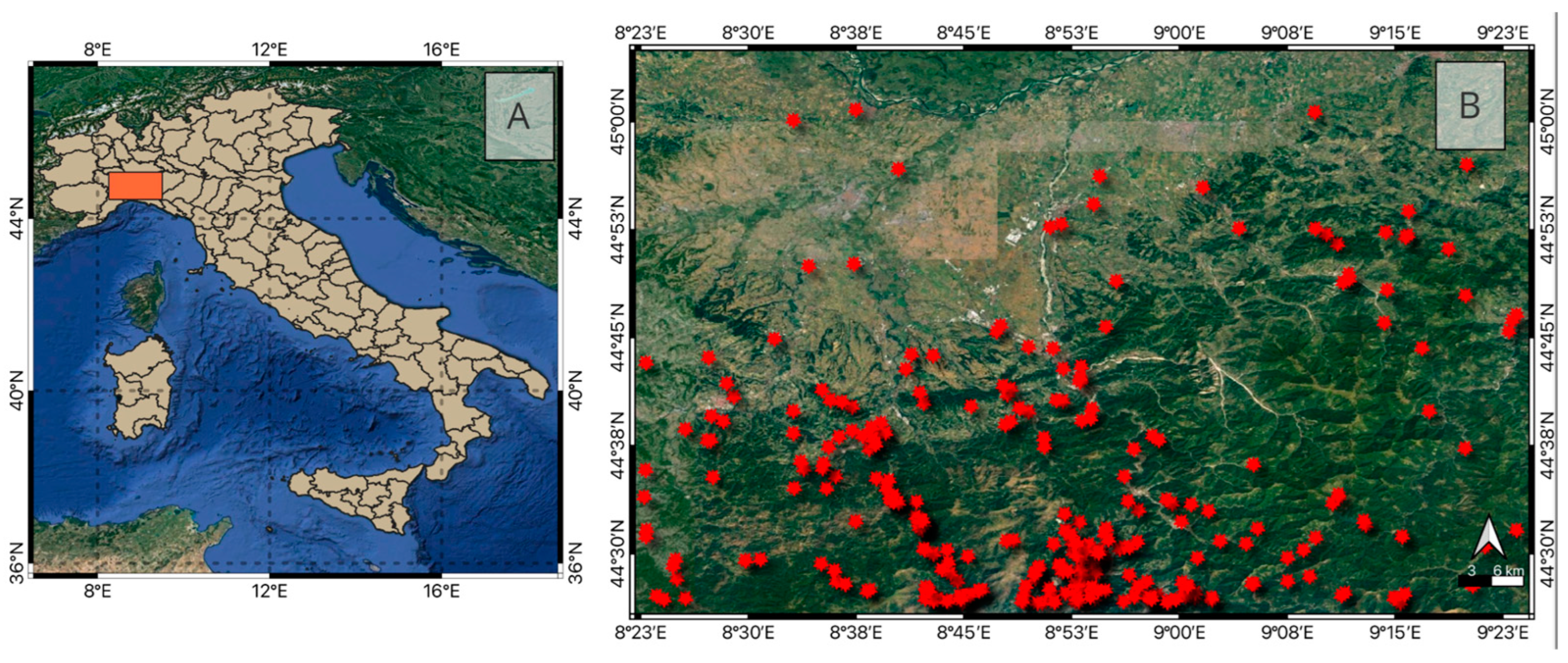
2. Study Area
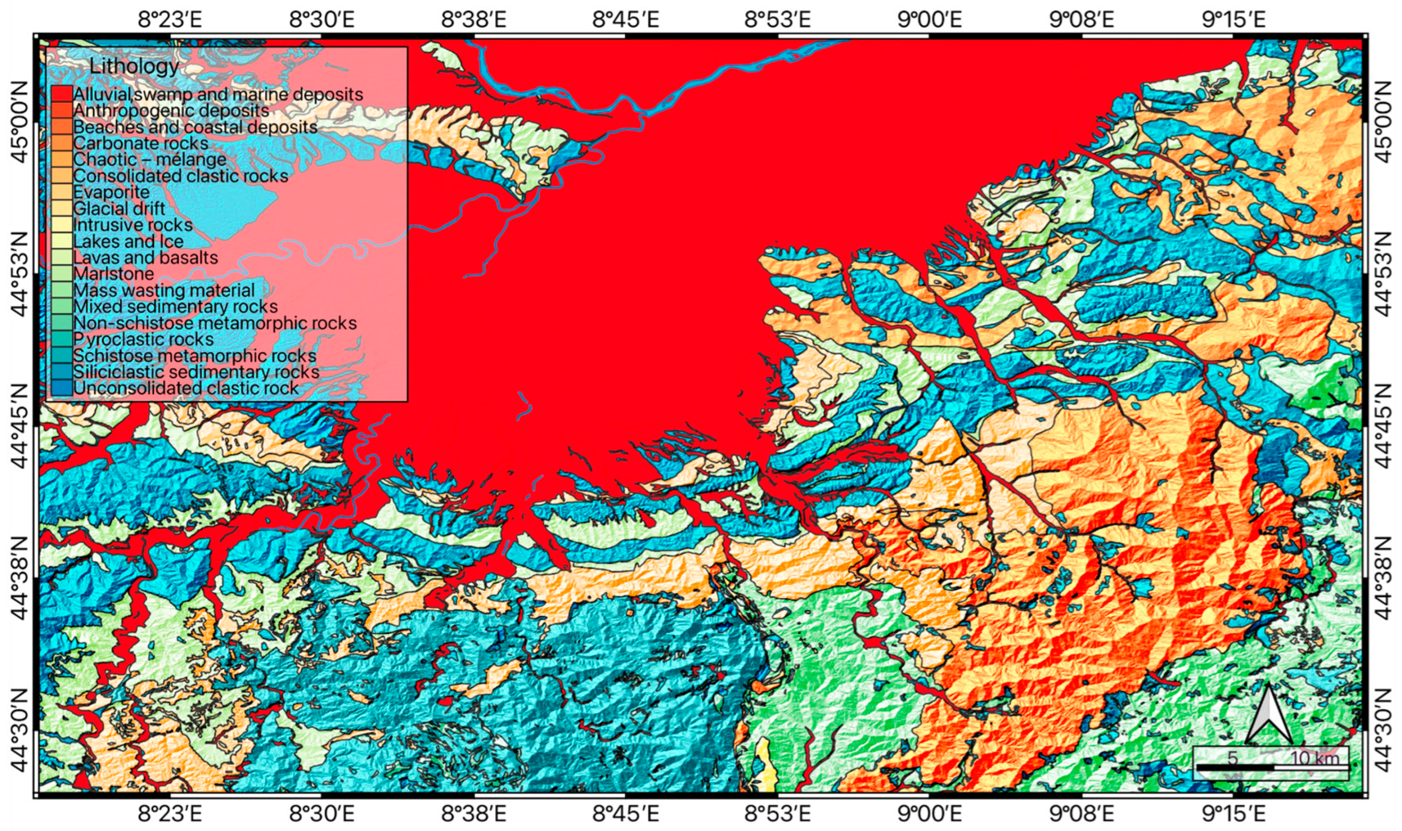
2.1. Geological and Geomorphological Setting
2.2. Climatic Features
3. Materials
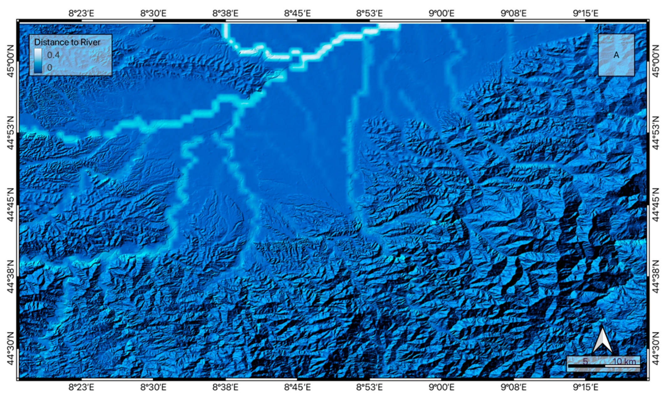
3.1. Static Conditioning Factors

3.2. Dynamic Conditioning Factors
4. Method
4.1. Machine Learning
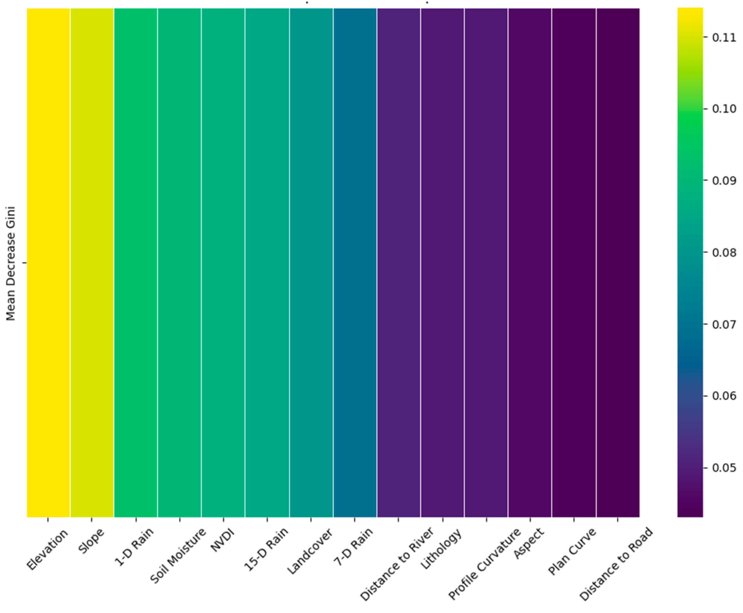
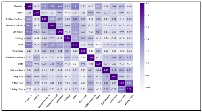
4.2. Relative Importance
5. Results and Discussion
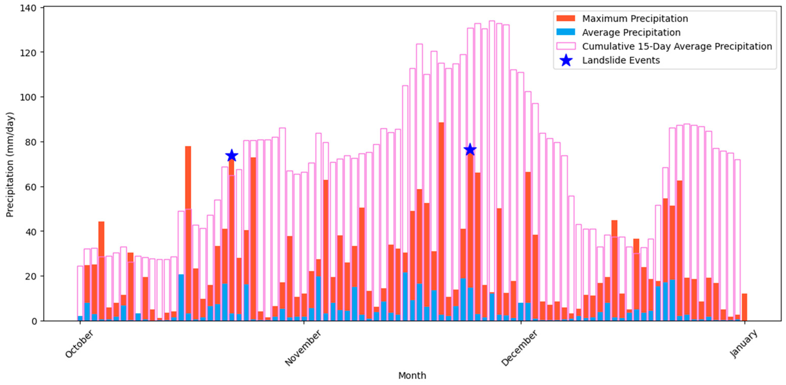
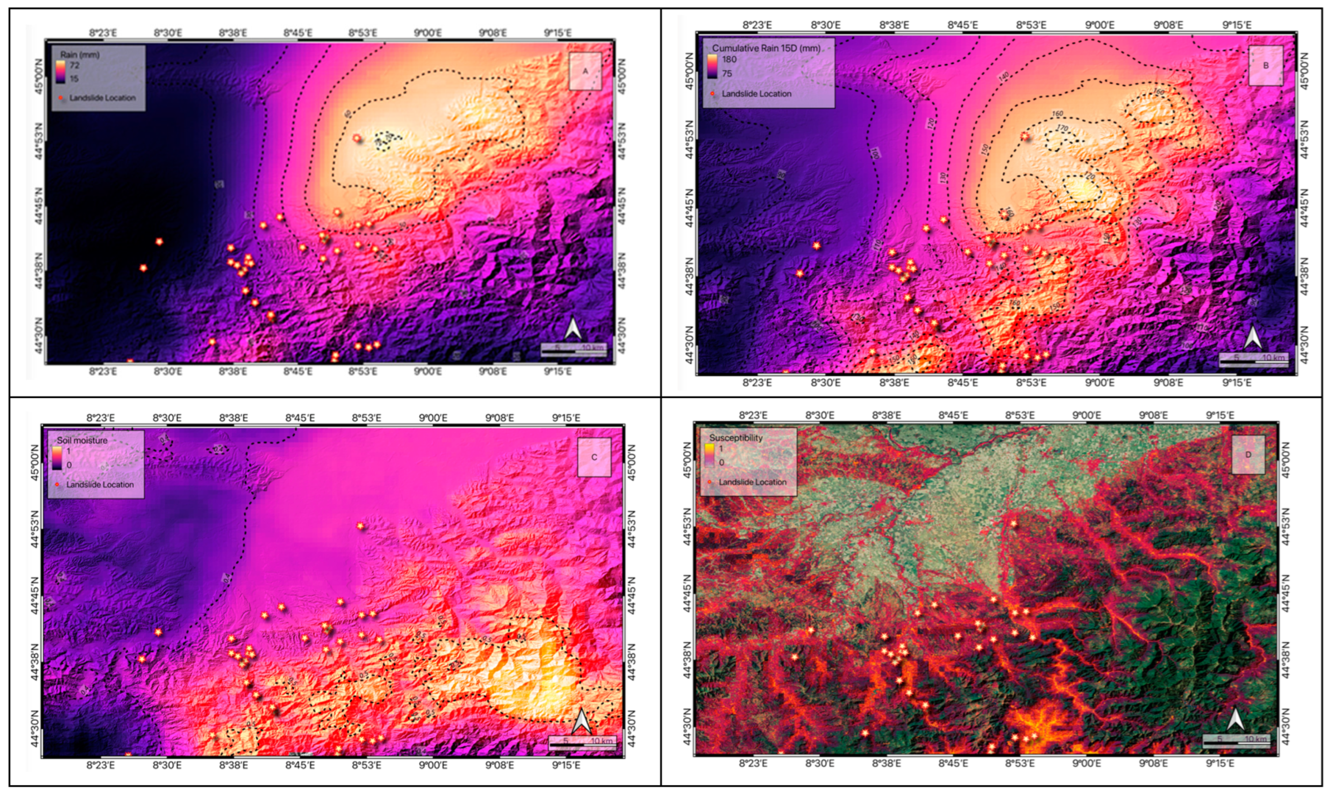
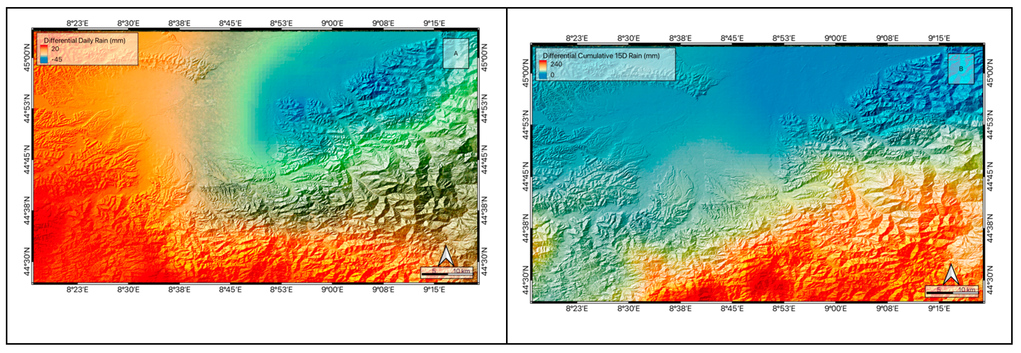
5.1. Rainfall Events
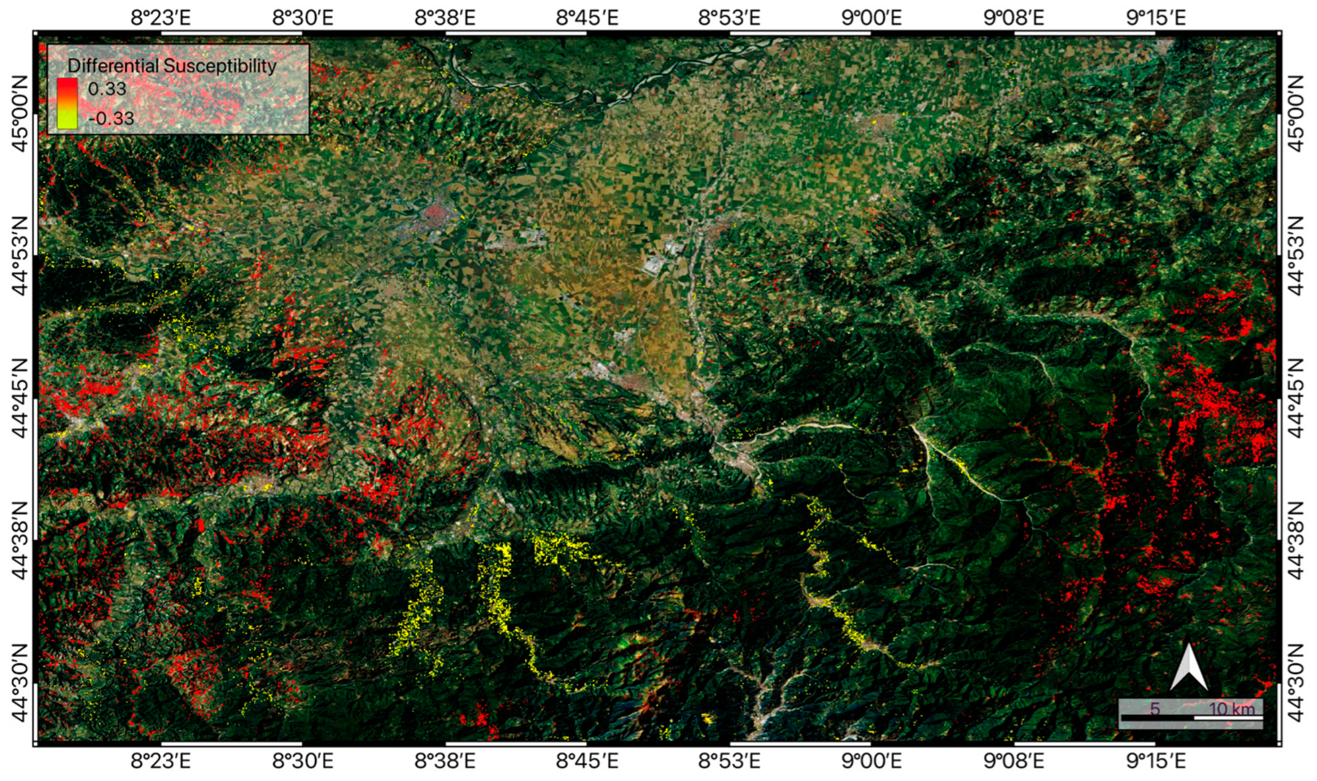
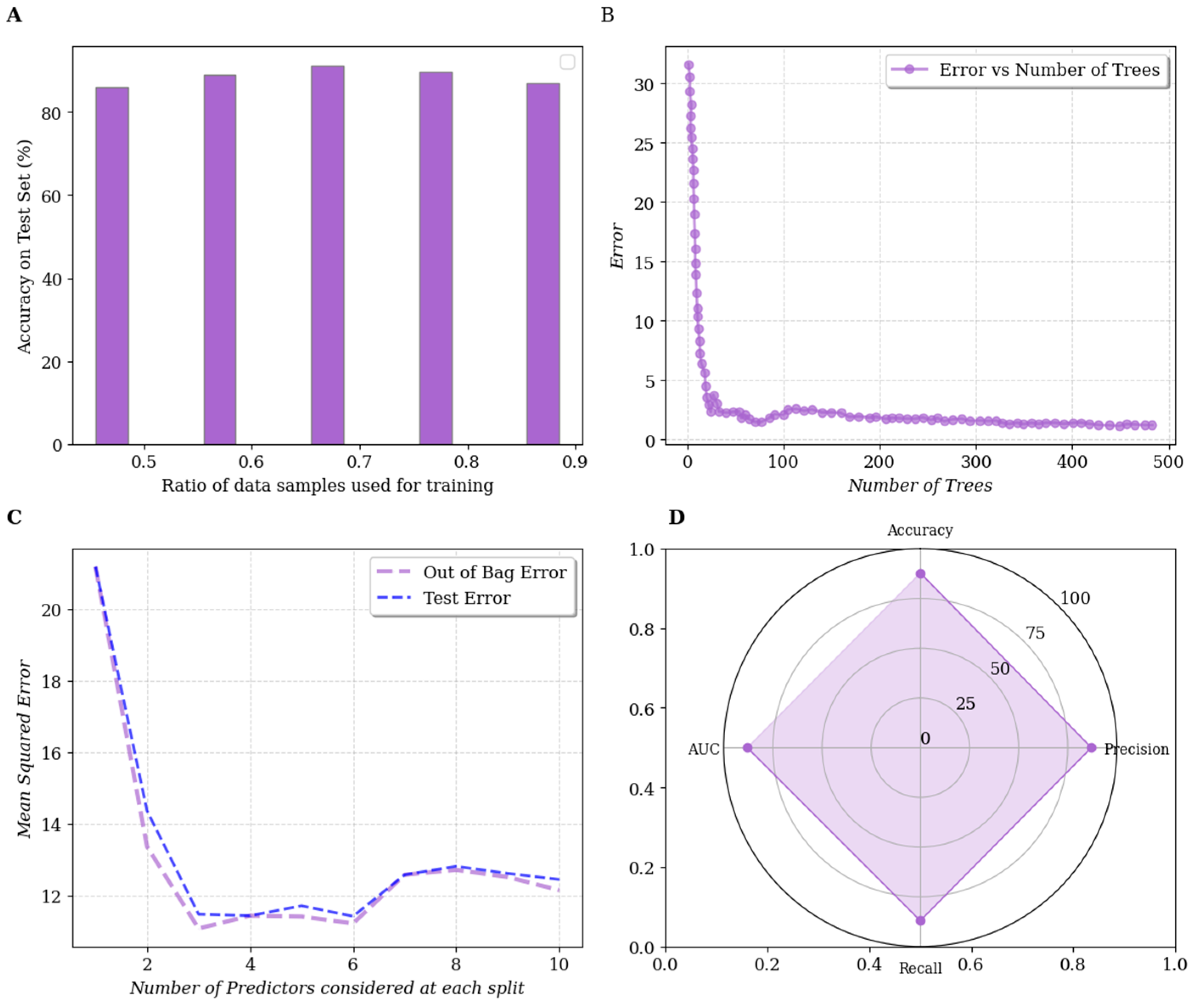
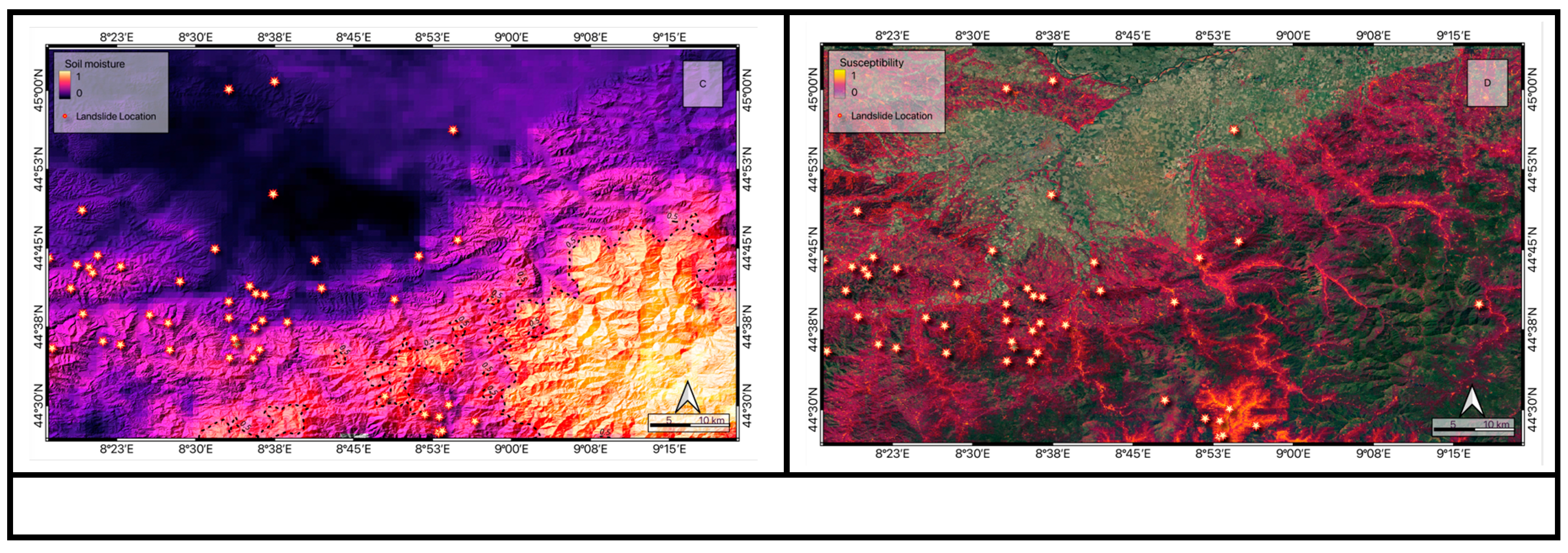
5.2. Modeling Results
5.3. Reliability Results
5.4. Conclusions
Acknowledgments
References
- F. Ardizzone, S.L. Gariano, E. Volpe, L. Antronico, R. Coscarelli, M. Manunta, A.C. Mondini, A Procedure for the Quantitative Comparison of Rainfall and DInSAR-Based Surface Displacement Time Series in Slow-Moving Landslides: A Case Study in Southern Italy, Remote Sensing 2023, 15, 320. [CrossRef]
- D. Salciarini, L. Brocca, S. Camici, L. Ciabatta, E. Volpe, R. Massini, C. Tamagnini, Physically based approach for rainfall-induced landslide projections in a changing climate, Proceedings of the Institution of Civil Engineers - Geotechnical Engineering 2019, 172, 481–495. [CrossRef]
- E. Volpe, S.L. Gariano, L. Ciabatta, Y. Peiro, E. Cattoni, Expected Changes in Rainfall-Induced Landslide Activity in an Italian Archaeological Area, Geosciences 2023, 13, 270. [CrossRef]
- E. Volpe, L. Ciabatta, D. Salciarini, S. Camici, E. Cattoni, L. Brocca, The Impact of Probability Density Functions Assessment on Model Performance for Slope Stability Analysis, Geosciences 2021, 11, 322. [CrossRef]
- D.S. Mwakapesa, X. Lan, Y. Mao, Landslide susceptibility assessment using deep learning considering unbalanced samples distribution, Heliyon 2024, 10, e30107. [CrossRef]
- G. Duan, J. Zhang, S. Zhang, Assessment of Landslide Susceptibility Based on Multiresolution Image Segmentation and Geological Factor Ratings, IJERPH 2020, 17, 7863. [CrossRef]
- J. Gao, X. Shi, L. Li, Z. Zhou, J. Wang, Assessment of Landslide Susceptibility Using Different Machine Learning Methods in Longnan City, China, Sustainability 2022, 14, 16716. [CrossRef]
- A. Trigila, C. Iadanza, C. Esposito, G. Scarascia-Mugnozza, Comparison of Logistic Regression and Random Forests techniques for shallow landslide susceptibility assessment in Giampilieri (NE Sicily, Italy), Geomorphology 2015, 249, 119–136. [CrossRef]
- W. Chen, W. Li, H. Chai, E. Hou, X. Li, X. Ding, GIS-based landslide susceptibility mapping using analytical hierarchy process (AHP) and certainty factor (CF) models for the Baozhong region of Baoji City, China, Environ Earth Sci 2016, 75, 63. [CrossRef]
- J. Dou, A.P. Yunus, D. Tien Bui, A. Merghadi, M. Sahana, Z. Zhu, C.-W. Chen, K. Khosravi, Y. Yang, B.T. Pham, Assessment of advanced random forest and decision tree algorithms for modeling rainfall-induced landslide susceptibility in the Izu-Oshima Volcanic Island, Japan, Science of The Total Environment 2019, 662, 332–346. [CrossRef]
- P. Aleotti, R. Chowdhury, Landslide hazard assessment: summary review and new perspectives, Bull Eng Geol Env 1999, 58, 21–44. [CrossRef]
- F. Guzzetti, A. Carrara, M. Cardinali, P. Reichenbach, Landslide hazard evaluation: a review of current techniques and their application in a multi-scale study, Central Italy, Geomorphology 1999, 31, 181–216. [CrossRef]
- A. Carrara, Multivariate models for landslide hazard evaluation, Mathematical Geology 1983, 15, 403–426. [CrossRef]
- D. Salciarini, R. Morbidelli, E. Cattoni, E. Volpe, Physical and numerical modelling of the response of slopes under different rainfalls, inclinations and vegetation conditions, RIG-2022-1-1 2022, 1229, 47–61. [CrossRef]
- D. Salciarini, E. Volpe, E. Cattoni, Probabilistic vs. Deterministic Approach in Landslide Triggering Prediction at Large–scale, in: F. Calvetti, F. Cotecchia, A. Galli, C. Jommi (Eds.), Geotechnical Research for Land Protection and Development, Springer International Publishing, Cham, 2020: pp. 62–70. [CrossRef]
- D. Salciarini, A. Lupattelli, F. Cecinato, E. Cattoni, E. Volpe, Static and seismic numerical analysis of a shallow landslide located in a vulnerable area, RIG-2022-2-2 2022, 1236, 5–23. [CrossRef]
- A. Johari, Y. Peiro, Determination of stochastic shear strength parameters of a real landslide by back analysis, IJRRS 2021, 4, 7–16. [CrossRef]
- A. Merghadi, A.P. Yunus, J. Dou, J. Whiteley, B. ThaiPham, D.T. Bui, R. Avtar, B. Abderrahmane, Machine learning methods for landslide susceptibility studies: A comparative overview of algorithm performance, Earth-Science Reviews 2020, 207, 103225. [CrossRef]
- J.N. Goetz, A. Brenning, H. Petschko, P. Leopold, Evaluating machine learning and statistical prediction techniques for landslide susceptibility modeling, Computers & Geosciences 2015, 81, 1–11. [CrossRef]
- A.M. Youssef, B.A. El-Haddad, H.D. Skilodimou, G.D. Bathrellos, F. Golkar, H.R. Pourghasemi, Landslide susceptibility, ensemble machine learning, and accuracy methods in the southern Sinai Peninsula, Egypt: Assessment and Mapping, Nat Hazards (2024). [CrossRef]
- N. Sharma, M. Saharia, G.V. Ramana, High resolution landslide susceptibility mapping using ensemble machine learning and geospatial big data, CATENA 2024, 235, 107653. [CrossRef]
- F. Huang, J. Zhang, C. Zhou, Y. Wang, J. Huang, L. Zhu, A deep learning algorithm using a fully connected sparse autoencoder neural network for landslide susceptibility prediction, Landslides 2020, 17, 217–229. [CrossRef]
- J. Yao, S. Qin, S. Qiao, W. Che, Y. Chen, G. Su, Q. Miao, Assessment of Landslide Susceptibility Combining Deep Learning with Semi-Supervised Learning in Jiaohe County, Jilin Province, China, Applied Sciences 2020, 10, 5640. [CrossRef]
- D. Tien Bui, A. Shirzadi, H. Shahabi, M. Geertsema, E. Omidvar, J. Clague, B. Thai Pham, J. Dou, D. Talebpour Asl, B. Bin Ahmad, S. Lee, New Ensemble Models for Shallow Landslide Susceptibility Modeling in a Semi-Arid Watershed, Forests 2019, 10, 743. [CrossRef]
- B.T. Pham, I. Prakash, J. Dou, S.K. Singh, P.T. Trinh, H.T. Tran, T.M. Le, T. Van Phong, D.K. Khoi, A. Shirzadi, D.T. Bui, A novel hybrid approach of landslide susceptibility modelling using rotation forest ensemble and different base classifiers, Geocarto International 2020, 35, 1267–1292. [CrossRef]
- C. Wang, H. Jia, S. Zhang, Z. Ma, X. Wang, A dynamic evaluation method for slope safety with monitoring information based on a hybrid intelligence algorithm, Computers and Geotechnics 2023, 164, 105772. [CrossRef]
- M.D. Ferentinou, M.G. Sakellariou, Computational intelligence tools for the prediction of slope performance, Computers and Geotechnics 2007, 34, 362–384. [CrossRef]
- N. Wang, H. Zhang, A. Dahal, W. Cheng, M. Zhao, L. Lombardo, On the use of explainable AI for susceptibility modeling: Examining the spatial pattern of SHAP values, Geoscience Frontiers 2024, 15, 101800. [CrossRef]
- L. Breiman, No title found., Machine Learning 2001, 45, 5–32. [CrossRef]
- K. Xu, Z. Zhao, W. Chen, J. Ma, F. Liu, Y. Zhang, Z. Ren, Comparative study on landslide susceptibility mapping based on different ratios of training samples and testing samples by using RF and FR-RF models, Natural Hazards Research 2024, 4, 62–74. [CrossRef]
- D.R. Cutler, T.C. Edwards, K.H. Beard, A. Cutler, K.T. Hess, J. Gibson, J.J. Lawler, RANDOM FORESTS FOR CLASSIFICATION IN ECOLOGY, Ecology 2007, 88, 2783–2792. [CrossRef]
- W. Chen, X. Xie, J. Wang, B. Pradhan, H. Hong, D.T. Bui, Z. Duan, J. Ma, A comparative study of logistic model tree, random forest, and classification and regression tree models for spatial prediction of landslide susceptibility, CATENA 2017, 151, 147–160. [CrossRef]
- P. Reichenbach, M. Rossi, B.D. Malamud, M. Mihir, F. Guzzetti, A review of statistically-based landslide susceptibility models, Earth-Science Reviews 2018, 180, 60–91. [CrossRef]
- P. Vorpahl, H. Elsenbeer, M. Märker, B. Schröder, How can statistical models help to determine driving factors of landslides?, Ecological Modelling 2012, 239, 27–39. [CrossRef]
- A. Brenning, Spatial prediction models for landslide hazards: review, comparison and evaluation, Nat. Hazards Earth Syst. Sci. 2005, 5, 853–862. [CrossRef]
- P. Reichenbach, M. Rossi, B.D. Malamud, M. Mihir, F. Guzzetti, A review of statistically-based landslide susceptibility models, Earth-Science Reviews 2018, 180, 60–91. [CrossRef]
- F. Guzzetti, P. Reichenbach, M. Cardinali, M. Galli, F. Ardizzone, Probabilistic landslide hazard assessment at the basin scale, Geomorphology 2005, 72, 272–299. [CrossRef]
- M. Di Napoli, H. Tanyas, D. Castro-Camilo, D. Calcaterra, A. Cevasco, D. Di Martire, G. Pepe, P. Brandolini, L. Lombardo, On the estimation of landslide intensity, hazard and density via data-driven models, Nat Hazards 2023, 119, 1513–1530. [CrossRef]
- N. Wang, H. Zhang, A. Dahal, W. Cheng, M. Zhao, L. Lombardo, On the use of explainable AI for susceptibility modeling: Examining the spatial pattern of SHAP values, Geoscience Frontiers 2024, 15, 101800. [CrossRef]
- S. Steger, M. Moreno, A. Crespi, S. Luigi Gariano, M. Teresa Brunetti, M. Melillo, S. Peruccacci, F. Marra, L. De Vugt, T. Zieher, M. Rutzinger, V. Mair, M. Pittore, Adopting the margin of stability for space–time landslide prediction – A data-driven approach for generating spatial dynamic thresholds, Geoscience Frontiers 2024, 15, 101822. [CrossRef]
- P. Magliulo, A. Di Lisio, F. Russo, Comparison of GIS-based methodologies for the landslide susceptibility assessment, Geoinformatica 2009, 13, 253–265. [CrossRef]
- L. Shano, T.K. Raghuvanshi, M. Meten, Landslide susceptibility evaluation and hazard zonation techniques – a review, Geoenviron Disasters 2020, 7, 18. [CrossRef]
- P. Lima, S. Steger, T. Glade, F.G. Murillo-García, Literature review and bibliometric analysis on data-driven assessment of landslide susceptibility, J. Mt. Sci. 2022, 19, 1670–1698. [CrossRef]
- N. Nocentini, A. Rosi, S. Segoni, R. Fanti, Towards landslide space-time forecasting through machine learning: the influence of rainfall parameters and model setting, Front. Earth Sci. 2023, 11, 1152130. [CrossRef]
- A. Dahal, H. Tanyas, C. Van Westen, M. Van Der Meijde, P.M. Mai, R. Huser, L. Lombardo, Space–time landslide hazard modeling via Ensemble Neural Networks, Nat. Hazards Earth Syst. Sci. 2024, 24, 823–845. [CrossRef]
- J.-J. Lee, M.-S. Song, H.-S. Yun, S.-G. Yum, Dynamic landslide susceptibility analysis that combines rainfall period, accumulated rainfall, and geospatial information, Sci Rep 2022, 12, 18429. [CrossRef]
- M. Ahmed, H. Tanyas, R. Huser, A. Dahal, G. Titti, L. Borgatti, M. Francioni, L. Lombardo, Dynamic rainfall-induced landslide susceptibility: a step towards a unified forecasting system, (2023). [CrossRef]
- T. Halter, P. Lehmann, A. Wicki, J. Aaron, M. Stähli, Optimising landslide initiation modelling with high-resolution saturation prediction based on soil moisture monitoring data, Landslides (2024). [CrossRef]
- P. Marino, D.J. Peres, A. Cancelliere, R. Greco, T.A. Bogaard, Soil moisture information can improve shallow landslide forecasting using the hydrometeorological threshold approach, Landslides 2020, 17, 2041–2054. [CrossRef]
- L. Schilirò, G.M. Marmoni, M. Fiorucci, M. Pecci, G.S. Mugnozza, Preliminary insights from hydrological field monitoring for the evaluation of landslide triggering conditions over large areas, Nat Hazards 2023, 118, 1401–1426. [CrossRef]
- Y. Peiro, L. Y. Peiro, L. Ciabatta, E. Volpe, E. Cattoni, Spatiotemporal Modelling of Landslide Susceptibility Using Satellite Rainfall and Soil Moisture Products through Machine Learning Techniques, (2024). [CrossRef]
- Y. Sun, D. Wendi, D.E. Kim, S.-Y. Liong, Deriving intensity–duration–frequency (IDF) curves using downscaled in situ rainfall assimilated with remote sensing data, Geosci. Lett. 2019, 6, 17. [CrossRef]
- V. Basumatary, B. Sil, Generation of Rainfall Intensity-Duration-Frequency curves for the Barak River Basin, Meteorol. Hydrol. Water Manage. (2017). [CrossRef]
- A.C. Mondini, F. Guzzetti, M. Melillo, Deep learning forecast of rainfall-induced shallow landslides, Nat Commun 2023, 14, 2466. [CrossRef]
- M.C. Levy, A. Cohn, A.V. Lopes, S.E. Thompson, Addressing rainfall data selection uncertainty using connections between rainfall and streamflow, Sci Rep 2017, 7, 219. [CrossRef]
- M.T. Brunetti, M. Melillo, S.L. Gariano, L. Ciabatta, L. Brocca, G. Amarnath, S. Peruccacci, Satellite rainfall products outperform ground observations for landslide prediction in India, Hydrol. Earth Syst. Sci. 2021, 25, 3267–3279. [CrossRef]
- T. Pellarin, C. Román-Cascón, C. Baron, R. Bindlish, L. Brocca, P. Camberlin, D. Fernández-Prieto, Y.H. Kerr, C. Massari, G. Panthou, B. Perrimond, N. Philippon, G. Quantin, The Precipitation Inferred from Soil Moisture (PrISM) Near Real-Time Rainfall Product: Evaluation and Comparison, Remote Sensing 2020, 12, 481. [CrossRef]
- H. Yang, K. Hu, S. Zhang, S. Liu, Feasibility of satellite-based rainfall and soil moisture data in determining the triggering conditions of debris flow: The Jiangjia Gully (China) case study, Engineering Geology 2023, 315, 107041. [CrossRef]
- Y. Hong, R. Adler, G. Huffman, Evaluation of the potential of NASA multi-satellite precipitation analysis in global landslide hazard assessment, Geophysical Research Letters 2006, 33, 2006GL028010. [CrossRef]
- F. Bucci, M. Santangelo, L. Fongo, M. Alvioli, M. Cardinali, L. Melelli, I. Marchesini, A new digital lithological map of Italy at the 1:100 000 scale for geomechanical modelling, Earth Syst. Sci. Data 2022, 14, 4129–4151. [CrossRef]
- Po River Basin Authority, 2006., Caratteristiche del bacino del fiume Po e primo esame dell’ impatto ambientale delle attivitá umane sulle risorse idriche (Characteristics of Po River catchment and first investigation of the impact of human activities on water resources), (n.d.).
- R. Vezzoli, P. Mercogliano, S. Pecora, A.L. Zollo, C. Cacciamani, Hydrological simulation of Po River (North Italy) discharge under climate change scenarios using the RCM COSMO-CLM, Science of The Total Environment 2015, 521–522, 346–358. [CrossRef]
- Y. Achour, H.R. Pourghasemi, How do machine learning techniques help in increasing accuracy of landslide susceptibility maps?, Geoscience Frontiers 2020, 11, 871–883. [CrossRef]
- X. Chen, W. Chen, GIS-based landslide susceptibility assessment using optimized hybrid machine learning methods, CATENA 2021, 196, 104833. [CrossRef]
- I. Cantarino, M.A. Carrion, F. Goerlich, V. Martinez Ibañez, A ROC analysis-based classification method for landslide susceptibility maps, Landslides 2019, 16, 265–282. [CrossRef]
- E. Volpe, S.L. Gariano, F. Ardizzone, F. Fiorucci, D. Salciarini, A Heuristic Method to Evaluate the Effect of Soil Tillage on Slope Stability: A Pilot Case in Central Italy, Land 2022, 11, 912. [CrossRef]
- D. Salciarini, E. Volpe, L. Di Pietro, E. Cattoni, A Case-Study of Sustainable Countermeasures against Shallow Landslides in Central Italy, Geosciences 2020, 10, 130. [CrossRef]
- G.J. Huffman, D.T. Bolvin, D. Braithwaite, K.-L. Hsu, R.J. Joyce, C. Kidd, E.J. Nelkin, S. Sorooshian, E.F. Stocker, J. Tan, D.B. Wolff, P. Xie, Integrated Multi-satellite Retrievals for the Global Precipitation Measurement (GPM) Mission (IMERG), in: V. Levizzani, C. Kidd, D.B. Kirschbaum, C.D. Kummerow, K. Nakamura, F.J. Turk (Eds.), Satellite Precipitation Measurement, Springer International Publishing, Cham, 2020: pp. 343–353. [CrossRef]
- P. Xie, M. Chen, S. Yang, A. Yatagai, T. Hayasaka, Y. Fukushima, C. Liu, A Gauge-Based Analysis of Daily Precipitation over East Asia, Journal of Hydrometeorology 2007, 8, 607–626. [CrossRef]
- L. Brocca, L. Ciabatta, C. Massari, T. Moramarco, S. Hahn, S. Hasenauer, R. Kidd, W. Dorigo, W. Wagner, V. Levizzani, Soil as a natural rain gauge: Estimating global rainfall from satellite soil moisture data, JGR Atmospheres 2014, 119, 5128–5141. [CrossRef]
- P. Filippucci, High-resolution remote sensing for rainfall and river discharge estimation, 2022.
- H. Gholami, A. Mohammadifar, Novel deep learning hybrid models (CNN-GRU and DLDL-RF) for the susceptibility classification of dust sources in the Middle East: a global source, Sci Rep 2022, 12, 19342. [CrossRef]
- Corder, Gregory W and Foreman, Dale I, Nonparametric statistics: A step-by-step approach, John Wiley \& Sons, 2014.
- Jan Hauke, Tomasz Kossowski, COMPARISON OF VALUES OF PEARSON’S AND SPEARMAN’S CORRELATION COEFFICIENTS ON THE SAME SETS OF DATA, (2011).
- A. Garg, K. Tai, Comparison of statistical and machine learning methods in modelling of data with multicollinearity, IJMIC 2013, 18, 295. [CrossRef]
- N.-D. Hoang, D. Tien Bui, A Novel Relevance Vector Machine Classifier with Cuckoo Search Optimization for Spatial Prediction of Landslides, J. Comput. Civ. Eng. 2016, 30, 04016001. [CrossRef]
- H. Hong, W. Chen, C. Xu, A.M. Youssef, B. Pradhan, D. Tien Bui, Rainfall-induced landslide susceptibility assessment at the Chongren area (China) using frequency ratio, certainty factor, and index of entropy, Geocarto International 2016, 1–16. [CrossRef]
- W. Chen, X. Xie, J. Wang, B. Pradhan, H. Hong, D.T. Bui, Z. Duan, J. Ma, A comparative study of logistic model tree, random forest, and classification and regression tree models for spatial prediction of landslide susceptibility, CATENA 2017, 151, 147–160. [CrossRef]


| Product | Spatial Resolution | Temporal Resolution | Temporal coverage | Source |
| IMERG-LR | 0.1° | 0.5 hour | 2002 – to date | NASA |
| CPC | 0.5° | Daily | 1981 – to date | NOAA |
| SM2RAIN | 1 km | Daily | 2017 – 2022 | TUWIEN |
| Factor | Description | Surce,scale/resolution |
| Elevation | Digital elevation of the terrain surface | DTM, 10m |
| Slope angle | Angle of the slope inclination | DTM, 10m |
| Aspect | Compass direction of the slope exposure | DTM, 10m |
| Plan curvature | Curvature perpendicular to the slope, indicating concave or convex surface | DTM, 10m |
| Profile Curvature | Curvature parallel to the slope, indicating concave or convex surfaces | DTM, 10m |
| Geology | Lithology of the surface material | Geo-Map 1:100 000 |
| land cover | physical material on the surface of the Earth | CORINE Land Cover (CLC), 100 m |
| NVDI | An index to quantify the growth of green vegetation on land cover | Landsat 7, 10m |
| Distance to river | Distance to river | HyrdoSHED(SRTM),10m |
| Distance to road | Distance to road | CIESIN,10m |
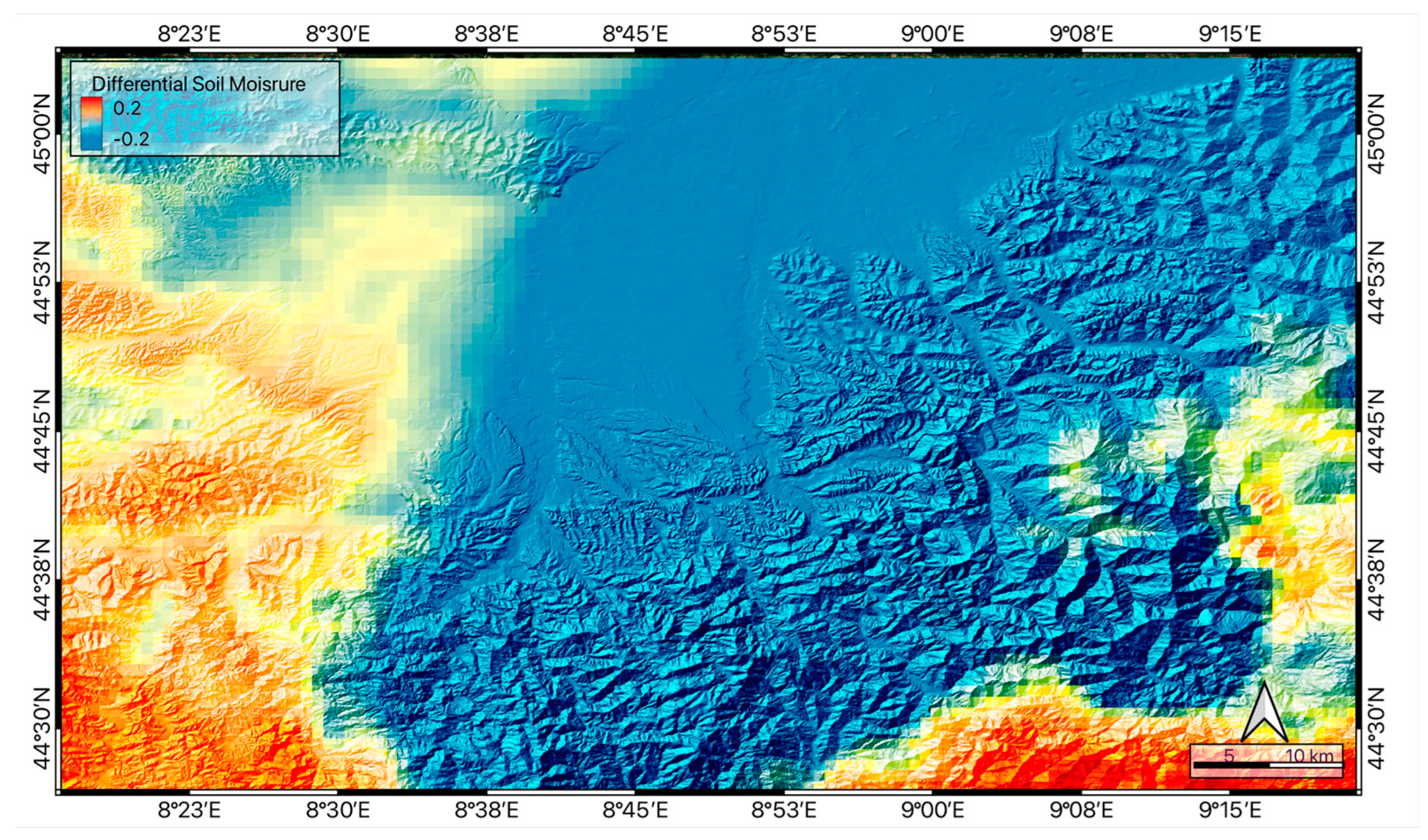
| Soil Moisture | Amount of soil water content | GLEAM 4DMED, 1Km |
| 1-Day Rain | Amount of cumulative 1-d antecedent rainfall | 4DMED, 1Km |
| 7-Day Rain | Amount of cumulative 7-d antecedent rainfall | 4DMED, 1Km |
| 15-Day Rain | Amount of cumulative 15-d antecedent rainfall | 4DMED, 1Km |
Disclaimer/Publisher’s Note: The statements, opinions and data contained in all publications are solely those of the individual author(s) and contributor(s) and not of MDPI and/or the editor(s). MDPI and/or the editor(s) disclaim responsibility for any injury to people or property resulting from any ideas, methods, instructions or products referred to in the content. |
© 2024 by the authors. Licensee MDPI, Basel, Switzerland. This article is an open access article distributed under the terms and conditions of the Creative Commons Attribution (CC BY) license (http://creativecommons.org/licenses/by/4.0/).


