Quantitative Evaluation of Reinforced Concrete Slab Bridges Using a Novel Bridge Health Index and LSTM-Based Deterioration Models

The Bridge Health Index (BHI) serves as an essential tool for assessing the structural and functional condition of bridges, calculated based on the condition of structural components and the serviceability of the bridge. Its primary purpose is to identify the most deteriorated structures in an asset inventory and prioritize those in most urgent need of repair. However, a frequently cited issue is the lack of accurate and objective data, with the determination of BHI often heavily reliant on expert opinions and engineering judgment. Furthermore, the BHI systems used in most countries are dependent on the current state of bridge components, making it challenging to use as a proactive indicator for factors such as the rate of bridge aging. To address this issue, this study introduces a novel BHI as a quantitative evaluation metric for reinforced concrete slab bridges and details the process of deriving the BHI based on deterioration models. The deterioration models are derived by preprocessing the deterioration data of reinforced concrete (RC) slab bridges, wherein the relationship between time and deterioration is directly employed for training a long short-term memory model. The BHI was validated through a case study involving six RC-slab bridges, wherein accuracies of >93% were achieved, confirming that the proposed quantitative evaluation methodology can significantly contribute to maintenance decisions for bridges.

Keywords:

Subject:

Engineering - Civil Engineering

1. Introduction

According to bridge-maintenance standards of several countries, including South Korea, the United States, and the United Kingdom [1,2,3,4], the maintenance procedure typically involves: 1) performing on-site inspections; 2) analyzing factors that impact bridge performance based on ultimate, service, and durability limit states; and 3) assessing the current performance level based on the analysis results. However, the amount of data required for the evaluation varies depending on the assessment level and significance, with insufficient data (e.g., material properties) substituted with values derived from statistical data and conservative assumptions. Although this method offers the advantages of prioritizing bridge maintenance and efficient allocation of personnel and costs, it faces limitations under a rapid increase in the number of aging bridges.

With the advent of the Fourth Industrial Revolution, various technologies have been explored to assess the current conditions of bridges, such as data acquisition through Internet-of-Things sensors, artificial intelligence (AI)-based analysis of the acquired data, virtual scenario analysis via simulation models, and the creation of digital twins by integrating virtual models with actual structures [5,6,7,8,9]. However, these methods assume that a sufficient budget and human resources are available for the target bridges, even though such levels of resources can be provided only for some bridges. Consequently, a more rational and quantitative bridge assessment method that does not deviate significantly from existing inspection frameworks is required for most bridges.

To address this issue, numerous machine-learning techniques have been proposed to track the current conditions of bridges based on past inspection and diagnostic data. Particularly in the United States, several studies have analyzed historical inspection data from the National Bridge Inventory to identify features that influence bridge-condition ratings (ranging from 0–9) and develop machine-learning models to predict them [10,11,12]. Among them, Assaad et al. [12] employed an artificial neural network (ANN) along with ten features to predict the conditions of bridge decks and achieved a prediction accuracy of 91.44%.

To incorporate more features that influence bridge-condition ratings, convolutional neural networks (CNNs), which are better suited than ANNs for learning high-dimensional data, have been considered [13,14,15]. ANNs process all features equally, whereas CNNs consider the relationships between features, resulting in highly accurate bridge-condition predictions when many features are employed. However, CNNs alone do not adequately consider the temporal characteristics of features, and research has been conducted to address this issue. Zhu et al. [16] developed a degradation model by combining a recurrent neural network (RNN) and CNN, and achieved prediction and conservative accuracies of over 80 and 85%, respectively, for the next three years.

Because RNNs process longer time histories, they encounter difficulties in converting information from earlier data to the current state. The long short-term memory (LSTM) algorithm was developed to address this issue, and some researchers have employed it to predict bridge-condition ratings [17,18,19]. Miao et al. [19] employed it to determine the cumulative effects of damage over time. Their model was trained on inspection data collected from 3,368 bridges in Japan, considering the potential factors influencing bridge deterioration (e.g., geometric characteristics, environmental factors, traffic conditions, and years of bridge use), which were categorized into deterioration grades (1–4). Subsequently, they built a deterioration-grade prediction model based on the deterioration factors and years of service and achieved accuracies exceeding 80%. Additionally, this result demonstrates that the LSTM model is superior to the multilayer perceptron model, which has an accuracy of 65%.

Most of the aforementioned data-driven deterioration-prediction models employ discrete data ranges because bridge-condition assessments worldwide are recorded in the form of categorical results, as listed in Table 1 [1,4,19,20,21,22,23,24]. This condition-rating system is widely used because it simplifies the reporting and determination of management priorities based on the bridge conditions. Several studies have employed this system as a foundation to predict future states of bridges. However, this approach can result in information loss and the disappearance of features by grouping continuous data based on the time history of damage. For instance, Choi et al. [17] compared the condition-rating predictions of various algorithms, including LSTM, linear regression, and deep neural networks, and demonstrated that their accuracies did not noticeably differ.

Additionally, an analysis of the bridge health index (BHI) employed by different countries [25] reveals that most indices, including the condition index based on condition ratings, depend primarily on the current state of the structural components, without accounting for performance indicators related to operation, safety, and life-cycle costs. This method proves insufficient for proactive measures, such as assessing the rate of bridge deterioration. A more effective BHI should incorporate metrics addressing various limit states, including utility, operational efficiency, and serviceability.

Therefore, in this study, a novel BHI as a quantitative evaluation metric for reinforced concrete slab bridges based on LSTM-based deterioration models was developed. Raw defect data obtained during bridge inspections were collected for training the LSTM, and a preprocessing procedure to reduce the uncertainty of bridge maintenance data was introduced in detail. The developed BHI was applied to six in-service RCS bridges to verify its effectiveness.

2. Materials and Methods

2.1. Data Collection

The maintenance guidelines in South Korea mandate that various activities related to the serviceability and durability of bridges must be conducted at specific intervals [1,4]. These activities are classified into "regular inspection," "precise inspection," "precise safety diagnosis," and "emergency inspection." In general, visual inspections are conducted to determine whether any defects have emerged since the previous “regular inspection,” and summary of the new defects is recorded. Consequently, the inspection data often contain significant human-induced uncertainties. Conversely, “precise inspection” and “precise safety diagnosis” are performed to identify physical and functional defects as well as inherent risk factors through field surveys and various tests. Figure 1 shows examples of slab defect map and quantity table recorded in an inspection report. This reporting method is essential for "precise inspection" and "precise safety diagnosis" to ensure that the types of defects, the year of occurrence, the volume of defects, and their locations can be accurately identified for each bridge component.

Because the inspection results contain quantifiable and abundant objective data, this study analyzed the inspection reports generated from "precise inspection" and "precise safety diagnosis" to collect the deterioration data. A total of 856 inspection reports pertaining to 311 reinforced concrete (RC)-slab bridges from nine regions (A–I) in South Korea were examined. The term "region" refers to 9 of the 17 administrative divisions in Korea, including the capital city, Seoul. This classification is necessary because bridge management agencies are designated based on administrative divisions, enabling the consideration of regional environmental factors, such as areas with high traffic volumes or regions prone to heavy snowfall.

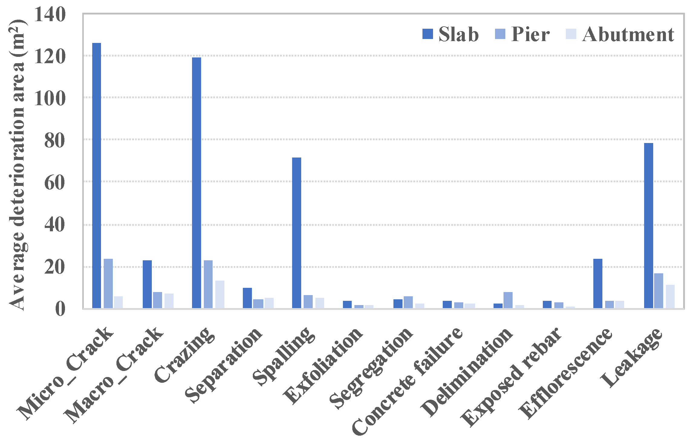
As the deterioration data in these inspection reports are categorized by components, individual data pertaining to slabs, piers, and abutments can be obtained. In total, 19,525 instances of 12 types of deterioration data were collected for each bridge component, as listed in Table 2. This categorization enabled distinguishing training data, allowing us to construct different deterioration models for each component, as described in Section 2.2. All data were collected in terms of area, and for one-way cracks, a width of 0.25 m was assumed to calculate the area. Additionally, the instances wherein the same type of deterioration was recorded at multiple locations within a component were aggregated and processed into a single data entry. Figure 2 shows the average area for each deterioration according to bridge components. The slab exhibits significantly higher occurrences of microcracks, macrocracks, crazing, spalling, efflorescence, and leakage than the other components, and it is evident that it experiences more damage owing to the direct impacts of moving vehicles.

2.2. LSTM-Driven Deterioration Model

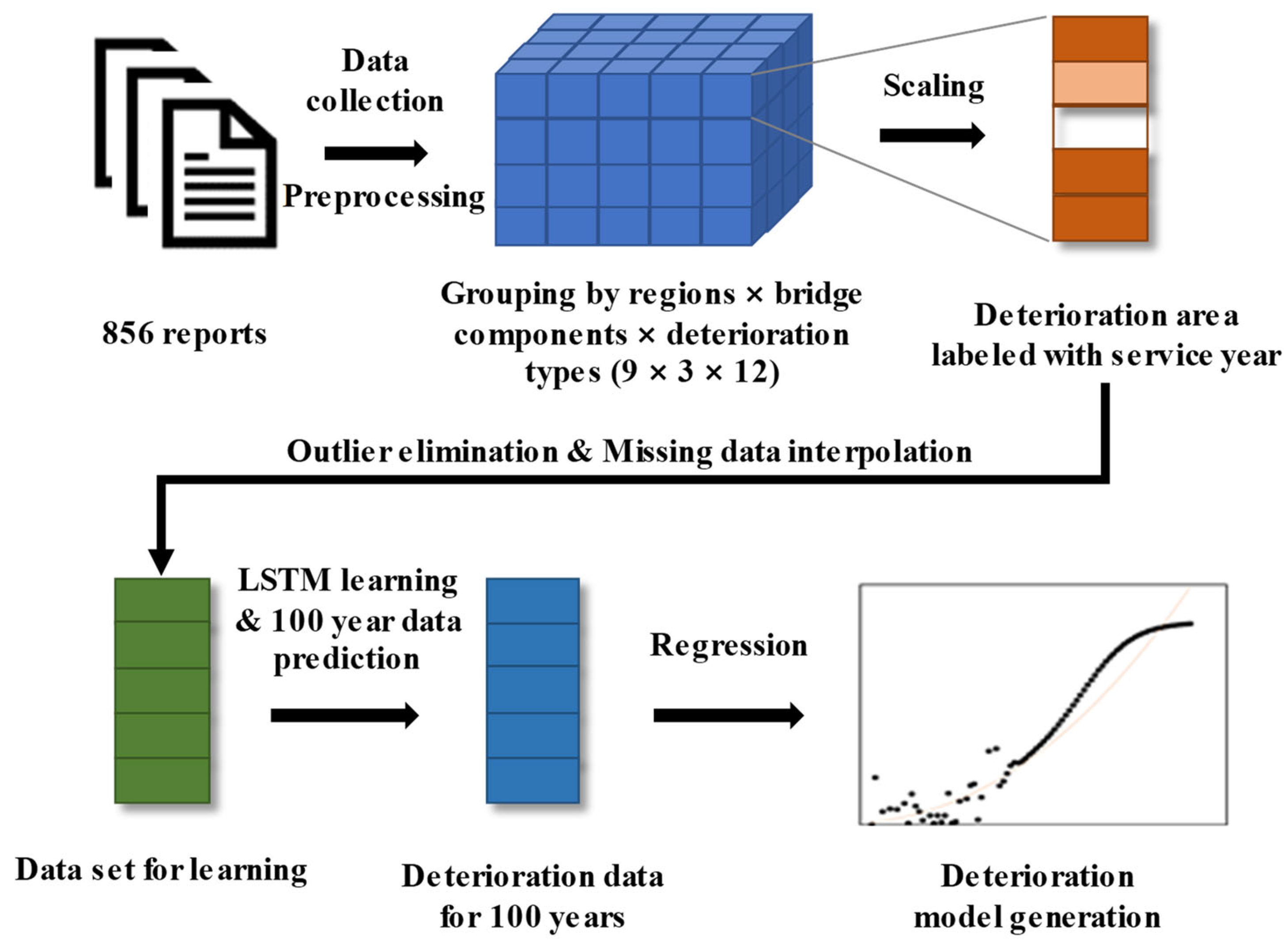
In a previous study [26], a carbonation deterioration model for RC-slab bridges was developed using the LSTM algorithm. Building on the same methodology, this study established deterioration models using the procedure illustrated in Figure 3. As described in Section 2.1, data collection involved gathering the necessary data from the bridge-inspection reports to train the deterioration model. During data pre-processing, the collected data were classified according to the 9 regions, 3 bridge components, and 12 deterioration types outlined in Table 2 to construct the training dataset, resulting in 324 datasets. This approach implies that the regional (environmental) characteristics and component type are not directly learned by the LSTM but are inherent within the 324 individually built datasets.

These 324 training sets were primarily constructed to ensure data continuity. When analyzing the deterioration data from maintenance reports, there were cases in which previously observed deterioration data appeared to be zero for certain years. Typically, this occurs when deteriorations, such as cracks, were detected during inspection in the previous year and repaired, resulting in no further deterioration being observed in the following inspection; hence, it was marked as zero. However, unless the underlying cause of the deterioration is addressed or the component is replaced, the deterioration generally persists. Therefore, these instances were corrected to retain the same values as those of the previous deterioration data. Additionally, if deteriorations were found in subsequent inspections, they were preprocessed and added to the previous data to ensure data accumulation.

As the collected data were aggregated by bridge component units, larger bridges tended to exhibited greater areas of deterioration. To mitigate this issue, the classified data were scaled according to bridge features (height, length, and width), as listed in Table 2, and calculated as follows:

A_{s c a l e d (t)}^{(i)} = \frac{\sum_{n} A_{d (t)}^{(i)}}{A_{c o m p .}}, i f \{\begin{matrix} S l a b : & A_{c o m p .} = L \times W \\ A b u t m e n t : & A_{c o m p .} = H \times W \\ P i e r & A_{c o m p .} = H \end{matrix}

(1)

For instance, if the service year of a bridge is

t

and the area of the

i

-th deterioration type within a single component is inspected

n

times, the total deterioration area

\sum_{n} A_{d (t)}^{(i)}

is calculated by summing all deterioration areas. Dividing the total deterioration area by the area of component,

A_{c o m p .}

, yields the scaled area of the

i

-th deterioration

A_{s c a l e d (t)}^{(i)}

. Additionally, if the target component is a deck,

A_{c o m p .}

is calculated as the product of total length (

L

) and width (

W

). For abutments,

A_{c o m p .}

is calculated as the product of mean height (

H

) and width (

W

). In the case of piers, scaling by area can sometimes lead to underestimations owing to their variety. Therefore,

A_{c o m p .}

for piers only considers the mean height (

H

The scaled data sets were classified based on the bridge-service life according to each data inspection point, thereby defining them as a time-series dataset. However, this dataset could be directly used for LSTM training owing to several reasons. The first was the presence of outliers. Bridge deterioration typically increases proportionally with the service life, except in the case of special or poorly maintained bridges. However, the measured data can be affected by human errors owing to the perspective and subjectivity of the inspectors. Therefore, this study employed the interquartile range, isolation forest, and Bayesian neural network (BNN) to remove outliers. Notably, the BNN calculates the probability distribution of the data and selects the deterioration data within the 1-σ range for training. The second reason was the presence of missing values in the time-series dataset owing to instances of no inspections because of inspection intervals, which led to data gaps that required compensation. Because linear interpolation can disturb the feature characteristics, this study employed the BNN model to probabilistically fill in these data gaps. The third reason was data duplication as the data were not classified by bridges. Therefore, surveys of multiple bridges in the same year resulted in multiple deterioration data points for a single time step. In such cases, the mean value of these multiple data points for each time step was calculated and used as a substitute.

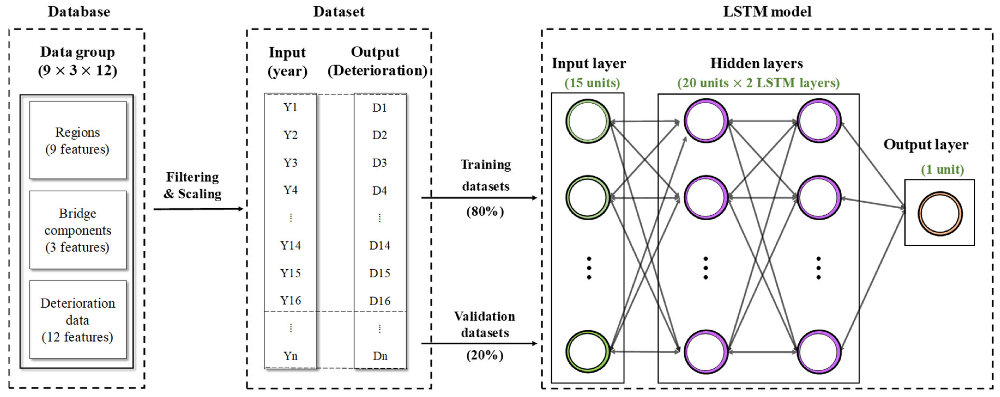
The dataset obtained through the aforementioned processes was used for the LSTM training, as shown in Figure 4. The TensorFlow library of Python was used for model building. Two LSTM layer were used as the learning model with the number of LSTM input data nodes set to 15. tanh was employed as the activation function for each layer and a dropout layer of 0.5 was added to each layer to prevent overfitting. During the learning process, the dataset was divided into training and validation sets. The validation data comprised data for the past decade from the initial dataset, whereas the training set included the remaining data. After model training was completed, the predictions for the past decade were compared with the samples in the validation set. However, the validation set contained observed values rather than true values, which introduced significant errors. Thus, a comparison was conducted using the average data values, and the average accuracy across all deterioration models was 76.8%.

The trained model was subsequently used to predict the deterioration data for each service year over the next 100 years. For example, if data were available up to the 35th service year, the LSTM model used the deterioration data from years 21–35 to predict deterioration in the 36th year. These data were then incorporated with those from years 22–35, and the LSTM model was used again to predict the data for the 37th year. This process was iterated to generate predictions for up to 100 years through each deterioration model. Finally, 324 datasets were generated, each containing deterioration data for up to 100 years.

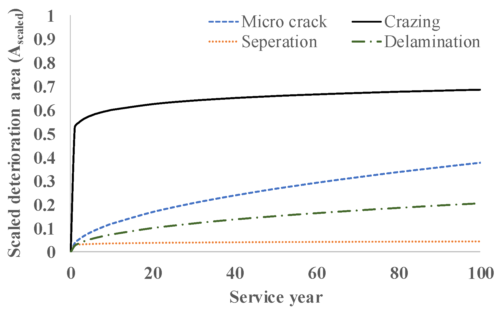
Regression analysis was then performed to derive the deterioration curve. In this study, a power-type trend equation (Eq. (2)) was used to describe the increase in the deterioration area over time (

t

), resulting in 324 deterioration models (

d^{1 ~ 324}

). Figure 5 presents an example of the 100-year deterioration results obtained for the slab components of RC slab bridges in Region A, showing the four most frequently observed types of deterioration (microcracks, crazing, separation, and delamination). Evidently, crack-related deterioration is expected to progress most rapidly in the RC-slab bridge within the region.

d_{(t)}^{(i)} = a t^{b}

(2)

2.3. Bridge Assessments Using Health Index

Each bridge component may exhibit multiple types of deterioration, which may have different effects on its performance level. Therefore, although the deterioration models derived in Section 2.2 reflect the deterioration progress over the service years based on the regional and structural characteristics, they cannot specifically reflect the current conditions. Furthermore, in cases wherein multiple deteriorations exist within a component, traditional maintenance standards typically evaluate each deterioration individually and assign the overall condition grade of the component to match the lowest deterioration grade. This approach poses the risk of significantly underestimating the performance level of a bridge and lacks quantitative evaluations.

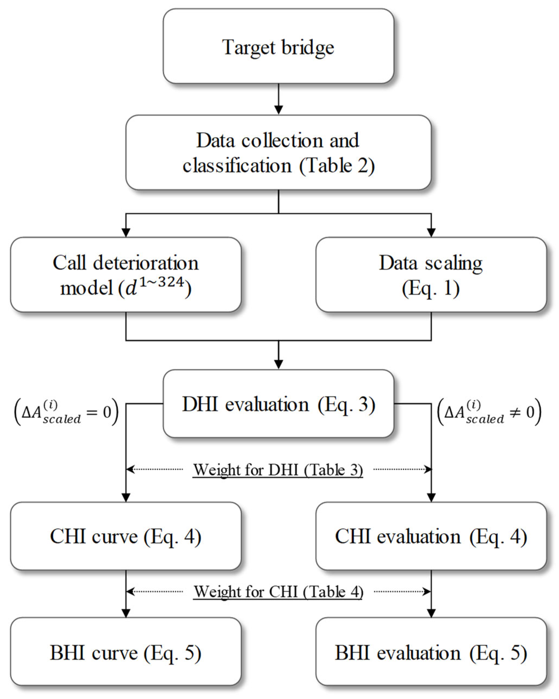
To address this issue, this study proposes the health index (HI) to quantitatively evaluate bridge conditions by incorporating the most recent damage information. As illustrated in Figure 6, the HI-derivation process involves three steps: 1) deriving the HI for each deterioration factor based on the deterioration curves in the database and general and environmental information of the target bridge, 2) aggregating and weighting the damage information for each component to derive the component-level HI, and 3) assigning weights to the components to derive the bridge-level HI.

2.3.1. Deterioration-Level HI (DHI)

Using the observed deterioration data for service year

t

, the DHI is calculated as follows:

{D H I}_{(t)}^{(i)} = 1 - \frac{{∆ A}_{s c a l e d}^{(i)} + d_{(t - 1)}^{(i)}}{d_{(100)}^{(i)}}

(3)

where

{D H I}_{(t)}^{(i)}

denotes the DHI for the

i

-th deterioration factor and

d_{(t - 1)}^{(i)}

denotes the deterioration value derived from the deterioration model for the

i

-th deterioration factor in the year immediately preceding the inspection year (

t - 1

). Additionally,

d_{(100)}^{(i)}

represents the threshold deterioration-level for the

i

-th deterioration factor, defined as the predicted damage for

t = 100

according to Eq. (1). Furthermore,

{∆ A}_{s c a l e d}^{(i)}

represents the increase in the scaled deterioration area compared to the inspection history data for each bridge component. For example, if the scaled deterioration area of a slab is 0.3 and 0.5 after 20 and 25 years of service life, respectively, then

{∆ A}_{s c a l e d}^{(i)}

= 0.2 (

A_{s c a l e d (25)}^{(i)} - A_{s c a l e d (20)}^{(i)} = 0.5 - 0.3 = 0.2

Eq. (3) indicates the extent to which the current damage level compares with the threshold service life. Thus, the PI represents the current performance level of the structure, which degrades over time owing to deterioration and damage relative to the target performance (safety and durability). A PI of zero indicates that the structure has reached the end of its service life. Moreover,

{∆ A}_{s c a l e d}^{(i)} = 0

in Figure 6 indicates that no new damage was found or considered. A PI curve that incorporates the regional and structural deterioration characteristics learned using the LSTM model can be derived by plotting a graph with t as the domain. Further details are presented in in Section 2.4.

2.3.2. Component-Level HI (CHI)

As mentioned previously, different types of deteriorations have different effects on the bridge-performance level. Therefore, weights must be assigned to each

{D H I}_{(t)}^{(i)}

in Figure 6 to derive the CHI. Because the weights for different deterioration types have not been established in maintenance standards or previous research, this study arbitrarily determined them based on the deterioration process. For a more detailed categorization, the deterioration factors affecting the structural safety of RC-slab bridges were classified into four modules: cracking, material, other, and corrosion defects (Table 3). According to previous studies on the deterioration process of RC-slab bridges [27], cracking defects, which include microcracks, macrocracks, and crazing, significantly affect bridge safety. If these defects continue to develop, they can lead to concrete peeling, punching shear failure, and rebar exposure. Therefore, this study considered that cracking and corrosion defects (exposed rebar) as accounting for 70% of the overall bridge deterioration, and exposed rebar is given a weight of 0.4 because it is the most significant deterioration factor in the deterioration process. Materials defects and other types defects do not directly affect the safety of the bridge but can contribute to performance degradation over time. As there is no clear evidence on which of these two factors has a greater impact on bridge aging, each was assigned a weight of 0.15.

Based on the weights listed in Table 3, the CHI for the

j

-th deterioration factor,

{C H I}_{(t)}^{(j)}

, was calculated as follows:

\begin{matrix} 0.3 (0.25 ∙ {D H I}_{(t)}^{(M i c r o c r a c k)} + 0.375 ∙ {D H I}_{(t)}^{(M a c r o c r a c k)} + 0.375 {D H I}_{(t)}^{(C r a z i n g)}) \\ {C H I}_{(t)}^{(j)} = + 0.15 (\begin{matrix} 0.167 ∙ {D H I}_{(t)}^{(S e p a r a t i o n)} + 0.167 ∙ {D H I}_{(t)}^{(S p a l l i n g)} \\ + 0.167 ∙ {D H I}_{(t)}^{(C o n c r e t e f a i l u r e)} + 0.167 ∙ {D H I}_{(t)}^{(E x f o l i a t i o n)} \\ + 0.167 ∙ {D H I}_{(t)}^{(S e g r e g a t i o n)} + 0.167 ∙ {D H I}_{(t)}^{(D e l a m i n a t i o n)} \end{matrix}) \\ + 0.15 (0.5 ∙ {D H I}_{(t)}^{(E f f l o r e s c e n c e)} + 0.5 ∙ {D H I}_{(t)}^{(L e a k a g e)}) \\ + 0.4 ∙ {D H I}_{(t)}^{(E x p o s e d r e b a r)} \end{matrix}

(4)

where

j

denotes the bridge component (slab, pier, or bridge).

2.3.3. Bridge-Level HI (BHI)

BHI is a key numerical indicator of the current performance level of a bridge. As discussed in Section 2.3.2, the

{C H I}_{(t)}^{(j)}

values are weighted accordingly. The current maintenance guidelines in South Korea provide weights for each component during the bridge-condition evaluation, and the component-specific weights for RC-slab bridges are listed in Table 4 [1,4].

Based on the weights (

ω_{j}

) listed in Table 4,

B {H I}_{(t)}

is calculated as follows:

{B H I}_{(t)} = 0.64 ∙ {C P I}_{(t)}^{(S l a b)} + 0.18 ∙ {C P I}_{(t)}^{(P i e r)} + 0.18 ∙ {C P I}_{(t)}^{(A b u t m e n t)}

(5)

2.4. Case Study

We conducted a case study by applying the proposed HI-based bridge evaluation method to actual bridges. Data of six RC-slab bridges located in urban areas, as listed in Table 5, were collected and their inspection reports were analyzed. These bridges were considered ideal for this study because they are located in high-traffic areas and are significantly affected by de-icing materials during winter. Furthermore, these bridges have been inspected multiple times at a minimum interval of two years, which facilitated data collection.

Table 6 presents the inspection history data for the case-study bridges. The service year, which was the primary feature for distinguishing the data, was evenly distributed from 16–45 years. For each service year, the extent of various types of deteriorations in the slabs, abutments, and piers were investigated. Note that only the numbers of newly discovered deteriorations compared with the previous service year are presented in Table 6. Additionally, material defects include six types of deteriorations (separation, spalling, concrete failure, exfoliation, segregation, and delamination), as listed in Table 3, and the total numbers of these deteriorations are listed in Table 6.

3. Results and Discussion

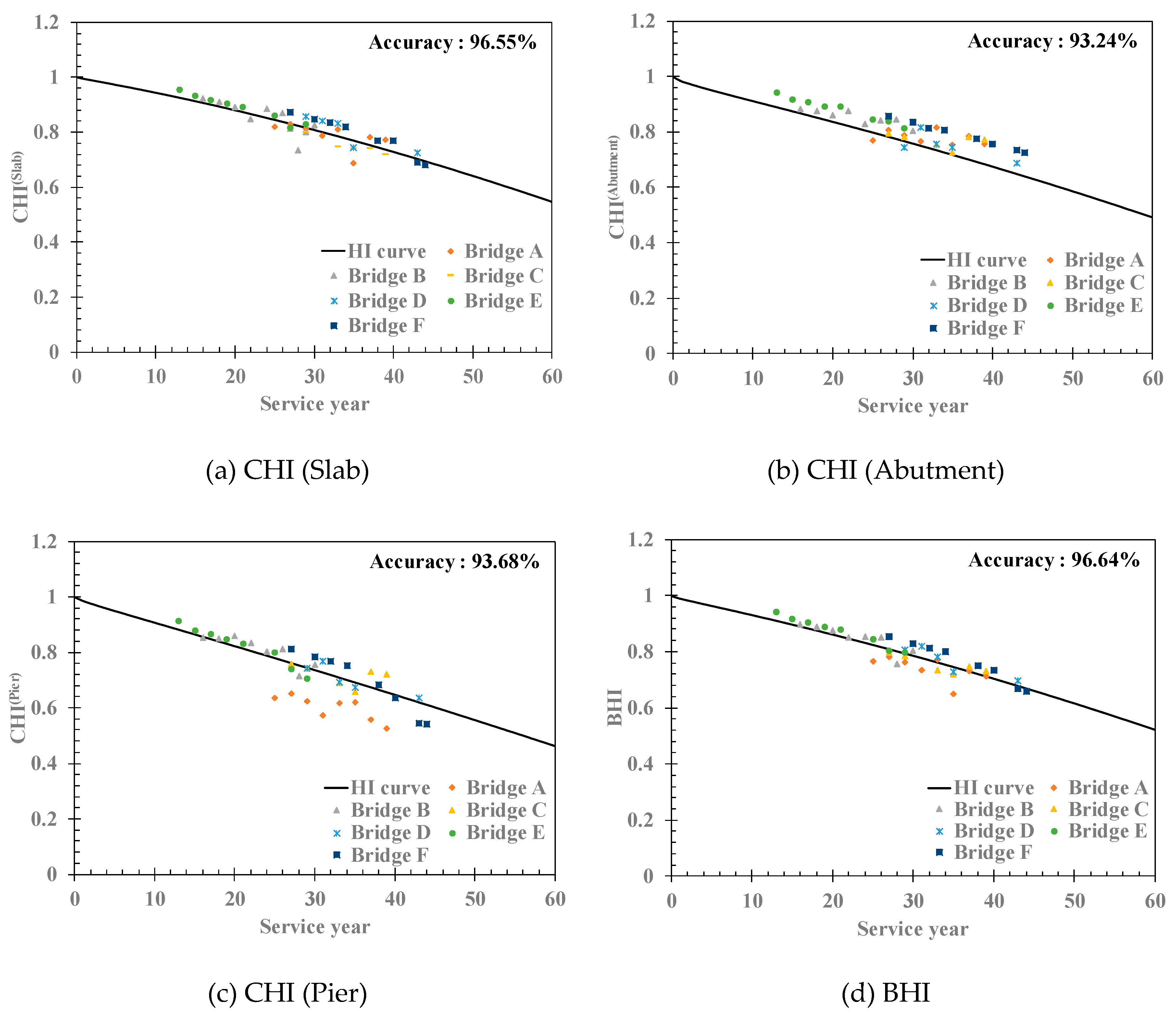
The results of applying the deterioration data in Table 6 and the HI-derivation procedure shown in Figure 6 are illustrated in Figure 7. The HI curve represents the trend of deriving the CHI and BHI using only the deterioration models derived in Section 2.2 without specifying a particular bridge. This curve can be derived by defining

{∆ A}_{s c a l e d}^{(i)}

as zero in Eq. (3) and then calculating the HI for each service year. It indicates the HI-change trend estimated from the deterioration information of RC-slab bridges in urban areas. To compare this curve with the HIs of the case-study bridges, the accuracy was derived using the following equation, and it exceeded 93% for all cases:

A c c u r a c y = \frac{1}{n} \sum_{1}^{n} |{H I}_{c a s e} - {H I}_{c u r v e}|

(6)

where

{H I}_{c a s e}

denotes the HI for the case-study bridges,

{H I}_{c u r v e}

denotes the HI obtained from the HI curve of Seoul without inspection data, and

n

denotes the number of

{H I}_{c a s e}

The results of our case study provided several insights. First, the alignment of the HI curves and trends for the case-study bridges suggests that the deterioration models outlined in Section 2.2 accurately reflect the specific deterioration characteristics of urban areas. Consequently, bridge-maintenance managers can estimate the performance degradation based on the bridge location even if detailed inspection information is unavailable. Second, the HI-based evaluation method can effectively visualize the extent of performance degradation. Significant deviations in the HIs of the bridges below the HI curve indicate higher levels of performance degradation compared with the regional average, whereas steep HI changes represent rapid increases in deterioration. For instance, in Figure 7(d), the results for Bridge A exemplify the former, whereas those for Bridge F exemplify the latter; these results can be used to make informed maintenance decisions. Bridge A requires more immediate attention than the other bridges owing to safety concerns, whereas Bridge F requires proactive measures to prevent further deterioration. Third, analyzing the HI of individual components can help identify targets for focused management. As shown in Figure 7(c), the pier of Bridge A has a particularly low HI, indicating a high level of deterioration, whereas that of Bridge F decreases rapidly. This suggests that, during inspections, the deterioration factors of piers in these bridges should be closely examined, and the necessary repairs should be conducted.

4. Conclusions

As bridges in most urban areas worldwide are aging, conducting preventive maintenance is essential to ensure their safety and reliability. However, conventional national bridge maintenance standards based on the HI are not suitable for accurately predicting how quickly bridges are aging because the HI is determined by the current condition. Therefore, this study developed a novel HI to quantitatively evaluate bridges by deriving deterioration models from inspection records using the LSTM algorithm. Inspection data from 865 bridge-inspection reports were used to train the LSTM model, resulting in 324 deterioration models that reflected 9 regions, 3 bridge components, and 12 deterioration types. These models were used to derive the DHI for each deterioration type of, and their CHI and BHI were derived through weighting, enabling quantitative evaluations.

In the case study, the HI curves of the deterioration models were compared with the HIs derived from actual inspection data of six bridges. Accuracies of >93% were confirmed for all bridges, thereby validating the effectiveness of the proposed HI- and LSTM-based bridge evaluation methodology. Additionally, the case-study results indicated that HI contributes to bridge-maintenance decisions by providing quantitative data and visual information regarding the level and rate of bridge deterioration.

Although this study specifically focused on RC-slab bridges, the proposed methodology can be applied to other types of bridges if sufficient data are available. However, owing to its considerable reliance on data, the reliability of the data is crucial, and pre-processing steps are required to eliminate human errors. The inspection data collected for this study exhibited significant variance, and data pre-processing was time-consuming. Additionally, regional characteristics were incorporated to derive the deterioration models. However, the application of more detailed environmental factors I expected to further enhance the reliability of these models, which is an important direction for future research.

Author Contributions

Conceptualization, J.K.; methodology, T.H.K. and J.K.; validation, C.-H.J., T.H.K. and J.K.; formal analysis, C.-H.J.; investigation, K.-S.J., C.-H.J., T.H.K. and J.K.; data curation, T.H.K.; writing—original draft preparation, C.-H.J.; writing—review and editing, C.-H.J.; visualization, C.-H.J. and T.H.K.; supervision, K.-T.P.; project administration, K.-S.J.; funding acquisition, K.-T.P. All authors have read and agreed to the published version of the manuscript.

Funding

Research for this paper was carried out under the KICT Research Program (project no. 20240142-001, Development of DNA-based smart maintenance platform and application technologies for aging bridges) funded by the Ministry of Science and ICT.

Data Availability Statement

All data, models, and code generated or used during the study are allowed under the permission of the corresponding author

Conflicts of Interest

The authors declare no conflicts of interest.

References

Korea Authority of Land and Infrastructure Safety (KALIS). Detailed Guideline for Safety and Maintenance Implementation of Facilities (Performance Evaluation); Korea Authority of Land and Infrastructure Safety (KALIS): Jinju, 2021. Available online: https://www.kalis.or.kr/www/brd/m_27/view.do?seq=117&srchFr=&srchTo=&srchWord=&srchTp=&itm_seq_1=0&itm_seq_2=0&multi_itm_seq=0&company_cd=&company_nm=.
American Association of State Highway and Transportation Officials (AASHTO). Manual for Bridge Evaluation with 2020 Interim Revisions; American Association of State Highway and Transportation Officials (AASHTO): Washington, DC, 2018. Available online: https://store.transportation.org/Item/CollectionDetail?ID=179.
Highways England. CS 454 Assessment of highway bridges and structures; Highways England: London, 2022. Available online: https://www.standardsforhighways.co.uk/dmrb/search/96569268-6c26-4263-a1f7-bc09a9e3977f.
Korea Authority of Land and Infrastructure Safety, (KALIS). Detailed Guideline for Safety and Maintenance Implementation of Facilities (Safety Inspection and Diagnosis); Korea Authority of Land and Infrastructure Safety (KALIS): Jinju, 2021. Available online: https://www.kalis.or.kr/www/brd/m_27/view.do?seq=117&srchFr=&srchTo=&srchWord=&srchTp=&itm_seq_1=0&itm_seq_2=0&multi_itm_seq=0&company_cd=&company_nm=.
Ritto, T. G. , & Rochinha, F. A. Digital twin, physics-based model, and machine learning applied to damage detection in structures. Mechanical Systems and Signal Processing 2021, 155. [Google Scholar] [CrossRef]
Mahmoodian, M. , Shahrivar, F., Setunge, S., & Mazaheri, S. Development of Digital Twin for Intelligent Maintenance of Civil Infrastructure. Development of Digital Twin for Intelligent Maintenance of Civil Infrastructure. Sustainability 2022, 14. [Google Scholar] [CrossRef]
Errandonea, I., Beltrán. Digital Twin for maintenance: A literature review. Computers in Industry 2020. [Google Scholar] [CrossRef]
Opoku, D. G. J., Perera. Digital twin application in the construction industry: A literature review. Journal of Building Engineering 2021. [Google Scholar] [CrossRef]
Jeon, C. H. , Shim, C. S., Lee, Y. H., & Schooling, J. Prescriptive maintenance of prestressed concrete bridges considering digital twin and key performance indicator. Engineering Structures 2024, 117383, 117383. [Google Scholar] [CrossRef]
Huang, Y.-H. Artificial Neural Network Model of Bridge Deterioration. Journal of Performance of Constructed Facilities 2010, 24, 597–602. [Google Scholar] [CrossRef]
Ali, G. , Elsayegh, A. , Assaad, R., El-Adaway, I. H., & Abotaleb, I. S. Artificial neural network model for bridge deterioration and assessment. In Proceedings of Canadian Society for Civil Engineering, June 2019. [Google Scholar]
Assaad, R., & El-adaway. Bridge Infrastructure Asset Management System: Comparative Computational Machine Learning Approach for Evaluating and Predicting Deck Deterioration Conditions. Journal of Infrastructure Systems 2020, 26, 1–17. [Google Scholar] [CrossRef]
Liu, H. , & Zhang, Y. Bridge condition rating data modeling using deep learning algorithm. Structure and Infrastructure Engineering, 2020, 16, 1447–1460. [Google Scholar] [CrossRef]
Kumar, A. , Singla, S., Kumar, A., Bansal, A., & Kaur, A.. Efficient Prediction of Bridge Conditions Using Modified Convolutional Neural Network. Wireless Personal Communications 2022, 125, 29–43. [Google Scholar] [CrossRef]
Fiorillo, G. , & Nassif, H. Improving the conversion accuracy between bridge element conditions and NBI ratings using deep convolutional neural networks. Structure and Infrastructure Engineering, 2020, 16, 1669–1682. [Google Scholar] [CrossRef]
Zhu, J. , & Wang, Y. Feature Selection and Deep Learning for Deterioration Prediction of the Bridges. Journal of Performance of Constructed Facilities 2021, 35. [Google Scholar] [CrossRef]
Choi, Y. , & Kong, J. Development of Data-based Hierarchical Learning Model for Predicting Condition Rating of Bridge Members over Time. KSCE Journal of Civil Engineering 2023, 27, 4406–4426. [Google Scholar] [CrossRef]
Saremi, S. G. , Goulias, D., & Zhao, Y. Alternative Sequence Classification of Neural Networks for Bridge Deck Condition Rating. Journal of Performance of Constructed Facilities 2023, 37, 1–15. [Google Scholar] [CrossRef]
Miao, P. , Yokota, H., & Zhang, Y. Deterioration prediction of existing concrete bridges using a LSTM recurrent neural network. Structure and Infrastructure Engineering 2023, 19, 475–489. [Google Scholar] [CrossRef]
Xia, Y. , Lei, X., Wang, P., & Sun, L. A data-driven approach for regional bridge condition assessment using inspection reports. Structural Control and Health Monitoring 2022, 29, 1–18. [Google Scholar] [CrossRef]
Federal Highway Administration (FHWA). Recording and coding guide for the structure inventory and appraisal ofthe nation’s bridges; FHWA: Washington, DC, 1995. [Google Scholar]
Highways Agency. DMRB Volume 3Section 1Part 4 (BD 63/07) Highway structures: Inspection and maintenance. 1 Part 4 (BD 63/07) Highway structures: Inspection and maintenance. 2007. Available online: https, 2007. Available online: https://www.thenbs.com/PublicationIndex/documents/details?Pub=HA&DocId=281590.
Hsien-Ke, L., Jallow. Comparison of bridge inspection methodologies and evaluation criteria in Taiwan and foreign practices. In Proceedings of the 34th International Symposium on Automation and Robotics in Construction; 2017; pp. 317–324. [Google Scholar] [CrossRef]
Roads, N. P., & Administration. Handbook for Bridge Inspections. online: https, 2005. Available online: https://www.tsp2.org/library-tsp2/uploads/48/Handbook_of_Bridge_Inspections_Part_1.pdf.
Chase, S. B., Adu-Gyamfi. Synthesis of National and International Methodologies Used for Bridge Health Indices. Federal Highway Administration. 1508. Available online: https://www.fhwa.dot.gov/publications/research/infrastructure/structures/bridge/15081/index.cfm.
Kwon, T. H. , Kim, J., Park, K. T., & Jung, K. S. Long Short-Term Memory-Based Methodology for Predicting Carbonation Models of Reinforced Concrete Slab Bridges: Case Study in South Korea. Applied Sciences 2022, 12. [Google Scholar] [CrossRef]
Fang, J. , Ishida, T., Fathalla, E., & Tsuchiya, S. Full-scale fatigue simulation of the deterioration mechanism of reinforced concrete road bridge slabs under dry and wet conditions. Engineering Structures 2021, 245, 112988. [Google Scholar] [CrossRef]

Figure 1. Example of a slab defect map and defect quantity table from the inspection report used for data collection.

Figure 2. Average deterioration areas for slabs, piers, and abutments.

Figure 3. Deterioration-model generation process.

Figure 4. Learning and validation processes for the proposed model.

Figure 5. Example of deterioration models for slab components in Region A.

Figure 6. HI-based bridge evaluation process.

Figure 7. HI plots for the case-study bridges.

Table 1. Bridge-condition rating systems employed in various countries.

Country	Condition rating	Description
U.S.	0–9	9: excellent, 0: fail
Denmark	0–5	0: insignificant deterioration, 5: no longer functional
Sweden	0–3	0: repair after 10 years, 3: repairs required now
Germany	0–4	0: defect has no effect, 4: structural strength is lost
Norway	1–4	1: minor damage, 4: critical damage
Japan	1–4	1: emergency action required, 4: healthy
England	1–5 (Severity)	1: no significant defects, 5: non-functional/fail
England	A–E (Extent)	A: no significant defects, E: >50% surface area affected
China	1–5	1: excellent, 5: fail
South Korea	A–E	A: excellent, E: fail

Table 2. Data extracted from inspection reports of RC-slab bridges.

Target components	Region	Type of deterioration data (measured by area, m²)	Bridge features
Slab Pier Abutment	Region A Region B Region C Region D Region E Region F Region G Region H Region I	Micro-crack (width < 0.03 mm) Macro-crack (width ≥ 0.03 mm) Crazing (two-way crack) Separation Spalling Exfoliation Segregation Concrete failure Delamination Efflorescence Leakage Exposed rebar	Height Width Length Service year

Table 3. Deterioration weight for DHI.

Deterioration type	Deterioration weight	Module	Module weight
Microcrack	0.25	Cracking defects	0.3
Macrocrack	0.375
Crazing	0.375
Separation	0.167	Materials defects	0.15
Spalling	0.167
Concrete failure	0.167
Exfoliation	0.167
Segregation	0.167
Delamination	0.167
Efflorescence	0.5	Other types of defects	0.15
Leakage	0.5	Other types of defects	0.15
Exposed rebar	1	Corrosion defect	0.4

Table 4. RC-slab bridge component weights for CHI

Bridge component	Weight
Slab	0.64
Pier	0.18
Abutment	0.18

Table 5. Bridges used for the case study.

Name	Construction year	No. of inspection reports	Width (m)	Length (m)	Height (m)
Bridge A	1978	8	30	34	6
Bridge B	1988	8	26	59	5
Bridge C	1987	7	40	31	4
Bridge D	1972	6	25	48	4
Bridge E	1981	6	30	47	4
Bridge F	1989	8	30	40	5

Table 6. Collected data from inspection records of case-study bridges.

Bridge	Service year	Component	Microcracks	Macrocracks	Crazing	Material defects	Efflorescence	Leakage	Rebar exposure
A	25	Slab	0.00	0.00	0.00	0.03	31.75	0.00	1.00
		Abutment	0.00	0.00	0.00	0.10	27.00	14.91	0.20
		Pier	5.90	0.90	0.00	15.84	0.00	11.80	0.00
	27	Slab	0.00	0.00	0.00	0.00	0.00	0.00	0.00
		Abutment	0.00	0.00	0.00	0.10	1.74	16.20	0.00
		Pier	0.30	0.60	0.00	0.60	0.10	0.00	0.00
	29	Slab	0.00	0.00	1.00	0.00	0.00	15.59	0.00
		Abutment	0.00	0.00	0.00	0.10	3.61	0.00	0.00
		Pier	0.30	0.60	0.00	0.01	0.00	0.00	0.00
	31	Slab	0.00	0.00	0.00	3.00	11.56	1.00	0.00
		Abutment	1.50	6.60	0.00	0.35	2.13	4.38	0.00
		Pier	1.50	6.60	0.00	6.76	2.13	4.38	0.00
	33	Slab	0.40	0.00	0.00	2.80	3.96	0.00	0.00
		Abutment	0.00	0.00	0.00	1.21	0.00	0.00	0.00
		Pier	0.00	0.00	0.00	3.32	0.00	0.00	0.00
	35	Slab	0.40	5.87	0.00	0.00	0.00	0.00	0.32
		Abutment	31.00	0.00	0.00	0.35	1.46	1.50	0.00
		Pier	5.80	2.00	0.00	18.31	0.00	0.00	0.00
	37	Slab	0.40	0.00	0.00	0.00	3.94	0.00	0.30
		Abutment	16.15	0.00	0.40	0.35	3.00	0.75	0.00
		Pier	16.15	0.00	0.40	4.95	3.00	0.75	0.00
	39	Slab	0.00	0.00	0.00	19.02	14.45	0.00	0.80
		Abutment	17.90	0.50	0.40	15.95	1.00	0.75	0.00
		Pier	17.90	0.50	0.40	17.35	1.00	0.75	0.00
B	16	Slab	49.70	44.10	0.00	0.00	0.00	0.00	0.00
		Abutment	5.24	10.88	0.00	0.00	0.05	0.36	3.06
		Pier	7.86	16.32	0.00	5.21	0.08	0.54	4.60
	18	Slab	0.00	0.00	0.00	0.00	0.00	0.00	0.00
		Abutment	0.00	0.00	0.00	0.00	0.00	0.00	0.00
		Pier	0.00	0.00	0.00	0.00	0.00	0.00	0.00
	20	Slab	45.40	5.40	0.00	2.12	41.17	0.00	0.00
		Abutment	4.28	2.64	0.00	2.79	0.05	1.80	0.00
		Pier	6.42	3.96	0.00	6.97	0.08	2.70	0.00
	22	Slab	326.20	511.20	0.00	2.12	41.17	0.00	0.00
		Abutment	4.28	2.64	0.20	5.58	0.05	1.80	0.00
		Pier	6.42	3.96	0.30	6.97	0.08	2.70	0.00
	24	Slab	32.40	0.00	0.00	2.45	0.02	0.00	0.00
		Abutment	19.70	6.90	0.00	5.59	0.00	2.70	0.00
		Pier	0.00	0.00	0.00	4.24	0.00	0.00	3.96
	26	Slab	2.53	0.00	0.00	3.59	2.80	0.00	0.00
		Abutment	6.50	5.90	0.00	6.09	0.00	2.88	0.00
		Pier	6.50	2.50	0.00	4.61	0.00	0.00	4.00
	28	Slab	35.80	0.00	1.50	82.19	0.01	0.00	0.00
		Abutment	10.50	5.20	1.40	10.01	0.00	3.24	0.00
		Pier	13.70	0.00	0.00	4.42	0.00	0.00	1.00
	30	Slab	24.50	0.00	31.50	32.48	0.08	0.00	0.00
		Abutment	35.70	12.70	1.40	10.12	0.06	2.20	0.00
		Pier	55.80	0.00	0.00	1.75	0.00	0.00	0.00
C	27	Slab	0.00	0.00	0.00	7.10	6.00	0.00	0.00
		Abutment	0.00	0.00	0.00	0.00	0.00	60.00	0.25
		Pier	0.00	0.00	0.00	3.00	0.00	3.00	0.00
	29	Slab	0.00	0.00	0.00	0.00	6.30	0.00	0.30
		Abutment	0.00	0.00	0.00	0.00	10.50	21.00	0.00
		Pier	0.00	0.00	0.00	0.00	0.00	0.00	0.00
	31	Slab	15.00	0.00	71.00	0.00	7.30	0.00	0.51
		Abutment	3.50	10.10	0.00	3.71	0.25	27.88	0.00
		Pier	3.50	10.10	0.00	31.83	0.25	27.88	0.00
	33	Slab	4.00	0.00	70.00	0.00	9.00	0.00	3.63
		Abutment	6.00	0.00	0.03	1.72	0.00	6.00	0.00
		Pier	2.00	0.00	0.39	7.59	0.00	6.00	0.00
	35	Slab	0.00	70.00	0.00	0.00	0.00	0.00	6.51
		Abutment	0.00	0.00	0.00	0.30	7.00	49.40	0.00
		Pier	0.00	0.00	0.00	9.29	3.70	0.00	5.00
	37	Slab	0.00	1.00	0.00	0.10	21.50	5.11	0.00
		Abutment	0.00	4.00	0.00	2.61	7.00	58.40	0.00
		Pier	0.00	0.00	0.00	19.95	0.20	7.50	0.00
	39	Slab	8.00	0.00	41.60	46.01	0.00	0.00	0.00
		Abutment	3.00	0.00	0.00	0.45	0.00	0.00	0.00
		Pier	0.00	0.00	0.00	0.00	0.00	0.00	0.00
	29	Slab	0.00	2.50	0.00	0.00	0.00	1.25	0.00
		Abutment	0.60	0.00	0.00	0.08	0.00	0.00	0.00
		Pier	0.00	0.00	0.00	4.77	0.00	4.60	0.00
D	31	Slab	3.00	3.50	21.00	0.00	0.00	0.00	0.00
		Abutment	1.80	0.00	0.00	30.80	0.60	0.00	0.00
		Pier	0.00	1.00	0.00	62.61	0.00	0.00	0.00
	33	Slab	0.00	0.00	0.00	0.00	0.00	0.00	0.00
		Abutment	0.00	0.00	0.00	5.57	0.00	0.00	0.00
		Pier	0.00	0.00	0.00	11.14	0.00	0.00	0.00
	35	Slab	0.00	0.00	8.00	0.00	0.00	0.00	27.40
		Abutment	0.00	0.00	0.00	0.52	0.00	10.80	0.00
		Pier	0.00	0.00	0.00	22.65	0.00	21.60	0.00
	43	Slab	0.00	0.00	0.00	0.00	28.89	0.00	2.50
		Abutment	0.00	0.33	0.00	2.40	3.73	0.00	0.67
		Pier	0.00	0.67	0.00	13.63	7.47	0.00	1.33
	45	Slab	0.00	0.00	0.00	0.00	67.29	0.00	4.15
		Abutment	0.00	0.00	2.00	0.18	0.00	0.00	0.00
		Pier	0.00	0.00	0.00	58.96	11.68	6.00	5.48
	26	Slab	2.53	0.00	0.00	3.59	2.80	0.00	0.00
		Abutment	6.50	5.90	0.00	6.09	0.00	2.88	0.00
		Pier	6.50	2.50	0.00	4.61	0.00	0.00	4.00
	28	Slab	35.80	0.00	1.50	82.19	0.01	0.00	0.00
		Abutment	10.50	5.20	1.40	10.01	0.00	3.24	0.00
		Pier	13.70	0.00	0.00	4.42	0.00	0.00	1.00
	30	Slab	24.50	0.00	31.50	32.48	0.08	0.00	0.00
		Abutment	35.70	12.70	1.40	10.12	0.06	2.20	0.00
		Pier	55.80	0.00	0.00	1.75	0.00	0.00	0.00
E	22	Slab	0.00	0.00	0.00	0.00	4.00	0.00	0.00
		Abutment	2.50	0.00	0.00	0.16	15.80	0.00	0.00
		Pier	0.00	0.00	0.00	0.00	0.00	0.00	0.00
	25	Slab	0.00	0.00	0.00	0.00	0.00	0.00	0.00
		Abutment	0.00	0.00	0.00	0.16	0.00	0.00	0.00
		Pier	0.00	0.00	0.00	0.00	0.00	0.00	0.00
	27	Slab	0.00	0.00	0.00	0.00	1.00	0.00	0.00
		Abutment	0.00	0.00	0.00	0.24	0.00	0.92	0.00
		Pier	0.00	0.00	0.00	2.00	0.00	1.83	0.00
	29	Slab	0.00	0.00	0.00	0.00	4.40	0.00	0.00
		Abutment	0.00	0.00	0.00	0.84	0.00	1.67	0.00
		Pier	0.00	0.00	0.00	4.53	0.00	3.33	0.00
	35	Slab	0.00	0.00	0.00	0.30	32.60	0.00	1.00
		Abutment	0.00	0.67	1.33	1.04	1.20	4.53	0.00
		Pier	0.00	1.33	2.67	13.07	2.40	9.07	0.00
	37	Slab	0.00	0.00	0.00	20.33	41.44	16.00	0.16
		Abutment	0.00	0.00	0.00	2.44	0.30	12.30	0.00
		Pier	16.70	0.00	0.00	1.78	0.00	0.00	0.00
	13	Slab	0.00	0.00	0.00	0.21	0.55	0.00	0.00
		Abutment	0.00	0.00	0.00	0.04	0.34	0.00	0.00
		Pier	7.65	0.40	0.00	1.66	0.98	0.00	0.00
	15	Slab	2.70	0.00	0.00	0.00	0.00	0.00	0.00
		Abutment	0.55	3.50	0.00	14.08	0.00	0.00	0.00
		Pier	0.55	3.50	0.00	14.04	0.00	0.00	0.00
F	17	Slab	2.57	2.50	0.00	0.00	0.00	0.00	0.00
		Abutment	2.20	0.50	0.00	3.48	0.00	0.00	0.00
		Pier	2.20	0.50	0.00	3.44	0.00	0.00	0.00
	19	Slab	2.57	0.00	0.00	0.00	0.00	0.00	0.00
		Abutment	1.70	0.50	0.00	8.78	0.00	0.00	0.00
		Pier	1.70	0.50	0.00	8.67	0.00	0.00	0.00
	21	Slab	36.80	4.60	0.00	2.54	0.30	0.00	0.00
		Abutment	6.10	1.65	0.00	0.34	0.00	0.00	0.00
		Pier	6.10	1.65	0.00	0.15	0.00	0.00	0.00
	25	Slab	59.40	2.50	0.00	3.87	7.01	0.00	0.02
		Abutment	21.40	0.00	0.00	3.19	0.00	15.00	0.00
		Pier	18.90	0.00	0.00	3.67	0.00	0.00	0.00
	27	Slab	58.50	3.00	0.00	3.87	0.41	0.00	0.00
		Abutment	21.70	0.00	0.00	6.54	0.00	0.87	0.10
		Pier	17.20	0.60	0.00	7.02	0.00	0.00	0.00
	29	Slab	22.60	1.50	0.00	48.00	0.25	0.00	0.00
		Abutment	0.00	0.00	0.00	7.14	0.00	0.57	0.00
		Pier	0.00	0.00	0.00	6.20	0.00	0.00	0.00
	28	Slab	35.80	0.00	1.50	82.19	0.01	0.00	0.00
		Abutment	10.50	5.20	1.40	10.01	0.00	3.24	0.00
		Pier	13.70	0.00	0.00	4.42	0.00	0.00	1.00
	30	Slab	24.50	0.00	31.50	32.48	0.08	0.00	0.00
		Abutment	35.70	12.70	1.40	10.12	0.06	2.20	0.00
		Pier	55.80	0.00	0.00	1.75	0.00	0.00	0.00

Disclaimer/Publisher’s Note: The statements, opinions and data contained in all publications are solely those of the individual author(s) and contributor(s) and not of MDPI and/or the editor(s). MDPI and/or the editor(s) disclaim responsibility for any injury to people or property resulting from any ideas, methods, instructions or products referred to in the content.

© 2024 by the authors. Licensee MDPI, Basel, Switzerland. This article is an open access article distributed under the terms and conditions of the Creative Commons Attribution (CC BY) license (http://creativecommons.org/licenses/by/4.0/).

Copyright: This open access article is published under a Creative Commons CC BY 4.0 license, which permit the free download, distribution, and reuse, provided that the author and preprint are cited in any reuse.

Alerts

MDPI Initiatives

Important Links

Choose an area of interest and we will send you notifications of new preprints at your preferred frequency.

Disclaimer

Quantitative Evaluation of Reinforced Concrete Slab Bridges Using a Novel Bridge Health Index and LSTM-Based Deterioration Models

Abstract

Keywords:

Subject:

1. Introduction

2. Materials and Methods

2.1. Data Collection

2.2. LSTM-Driven Deterioration Model

2.3. Bridge Assessments Using Health Index

2.3.1. Deterioration-Level HI (DHI)

2.3.2. Component-Level HI (CHI)

2.3.3. Bridge-Level HI (BHI)

2.4. Case Study

3. Results and Discussion

4. Conclusions

Author Contributions

Funding

Data Availability Statement

Conflicts of Interest

References

MDPI Initiatives

Important Links

Subscribe