
Submitted:
25 October 2024
Posted:
29 October 2024
You are already at the latest version
Preprints on COVID-19 and SARS-CoV-2
Abstract
The optimal power flow (OPF) problem is a critical component in the design and operation of power transmission systems. Various optimization algorithms have been developed to address this issue. This paper expands the use of the Coronavirus Disease Optimization Algorithm (COVIDOA) to solve a multi-objective OPF problem (MO-OPF), incorporating renewable energy sources as dis-tributed generation (DG) across multiple scenarios. The main objectives are to minimize fuel costs, emissions, voltage deviations, and power losses. Due to its non-convex nature and computational complexity, OPF poses significant challenges. While COVIDOA has been utilized to solve engi-neering problems, it faces difficulties with non-linear and non-convex issues. This paper introduces an enhanced version, the Enhanced COVID Optimization Algorithm (ENHCOVIDOA), designed to improve the performance of the original method. The effectiveness of the proposed algorithm is validated through testing on IEEE 30-bus and 57-bus systems, as well as a real-world 28-bus system representing Iraq’s Standard Iraq Super Grid High Voltage (SISGHV-28 Buses). The Two-Point Estimation Method (TPEM) is also applied to manage uncertainties in renewable energy sources in some cases, leading to cost reductions and annual savings of ($87772.9374, $391246.87, & $ 2,493,881.40) for the IEEE 30-bus, 57-bus, and reality 28-bus systems, respectively. Thirteen dif-ferent cases were analyzed, and the results demonstrate that ENHCOVIDOA is notably more ef-ficient and effective than other optimization algorithms in the literature.
Keywords:
Optimization Algorithm
; multi-objective OPF problem
; distributed generation
; TPEM
; Standard Iraq Super Grid High Voltage 28 Buses
1. Introduction
As the integration of renewable energy generation as DG units continues to rise in modern interconnected and restructured power systems, the significance of addressing optimal power flow problems has grown considerably. Optimal power flow outcomes are essential for the planning, economic operation, and control of current electrical power systems, as well as for planning future expansions [1]. Researchers have made significant progress in addressing OPF issues in electrical networks. OPF involves adjusting control variables like generator voltages, active power outputs, phase shifters, transformer tap settings, and reactive power sources to optimize certain objectives. Some of these variables are discrete, while others are continuous, making the OPF problem complex and non-convex, posing challenges for optimization techniques [2]. Integrating DG units is promising, and it's crucial to assess their impact on the power network. Proper placement and sizing of DGs affect power reliability, costs, voltage profiles, losses, pollution, and stability, making it a key focus for researchers and industry experts [3]. As power injection from DGs into the network increases, it becomes crucial to determine the optimal power generation and control settings to minimize fuel costs, emission costs, and real power losses while enhancing the voltage profile [4]. Recently, researchers have developed various population-based, random search algorithms that have proven to be effective for solving complex optimization problems. These population-based, random search algorithms are highly versatile, making them suitable for addressing a wide range of optimization challenges, including linear, nonlinear, and constrained problems. Some of these methods include the Gaussian bare-bones Levy-flight firefly algorithm (GBLFA) and its modified version MGBLFA [5], the multi-objective search group algorithm (MOSGA) [6], Rao algorithms [7], the interior search algorithm (ISA) [8], the multi-objective backtracking search algorithm (MOBSA) [9], and fuzzy adaptive hybrid self-adaptive particle swarm optimization with differential evolution algorithms such as FAHSPSO-DE, for addressing MO-OPF problems [10], among others. This paper introduces a new evolutionary optimization algorithm called the Enhanced Coronavirus Disease Optimization Algorithm (ENHCOVIDOA) to address the multi-objective optimal power flow problem, both with and without uncertainties related to DG sources such as solar and wind power also, it aimed to improving the performance of the original method COVIDOA in [11]. COVIDOA simulates the behavior of the corona virus as it invades human cells. Notably, most viruses follow similar stages in their replication process, including entry, uncoating, replication, assembly, and the release of new virions [12]. The presence of distribution generators and the possibility of their operation under conditions of uncertainty require us to use an effective method for dealing with uncertainty that balances between reducing the computational burden and accuracy, such as TPEM, the Two-Point Estimation Method is employed in this study to handle uncertain-ties and achieve multiple objectives in the optimal power flow problem [13]. In recent years, nonconventional energy sources have gained popularity due to their availability and the rapid depletion of fossil fuels. Renewable energy is also favored for being clean and environmentally friendly. However, integrating renewables into the OPF problem adds complexity due to the unpredictable nature of their generation, which fluctuates with changing natural conditions. Efficient operation of electrical networks is essential for integrating renewable energy sources like DG into power systems [14]. Along with the growing flexibility of power electronics-based renewables, various control strategies and optimization methods help maximize DG potential while ensuring system stability. To address uncertainties in wind and solar generation, probabilistic OPF can be formulated using methods such as the point estimate method [15], fuzzy OPF [16], Monte Carlo simulation (MCS) [17,18], and the cumulant method [19]. While MCS requires significant computational time, the cumulant method becomes more complex with additional variables. TPEM offers advantages in managing these challenges. There are many countries considered promising in the integration of renewable energy generators into their electrical power systems, and Iraq is one of them. Iraq's electrical system primarily depends on thermal and gas turbines, and there is a significant gap in studies addressing optimal energy flow targets, particularly in how these targets are influenced by renewable energy sources, which are inherently uncertain. Furthermore, there is a need to explore effective methods, such as the two-point estimation method, for managing the variability of renewable generation and accurately determining optimal flow targets. To address these challenges, this paper introduces an innovative approach that combines TPEM and ENHCOVIDOA to enhance multi-objective optimal power flow analysis. TPEM is used for modeling uncertainties, while ENHCOVIDOA is applied to identify optimal values for the objectives in the optimal power flow problem.
The main contributions of the paper can be briefly stated as follows:
- This paper introduces a novel and efficient population-based algorithm called ENHCOVIDOA, tailored to address the multi-objective operational cost function during the operation phase. The algorithm excels at handling the intricate trade-offs involved in the operation of generators and renewable energy sources (RES), including factors such as costs, emissions, network losses, and voltage deviations.
- The proposed algorithm is capable of solving a broad spectrum of OPF problems for IEEE 30-bus and 57-bus standard power systems, achieving better results than algorithms of other literature both with and without the presence of distributed generation.
- This study accounts for uncertainties in the output of RES while formulating the probabilistic MO-OPF problem, using TPEM to improve the accuracy of the objectives by calculating mean and standard deviation of objectives.
- Calculate the multi-objective OPF for a reality 28 buses system from Iraq and analyze the impact of renewable energy uncertainty on the system's objectives.
The structure of this paper is as follows: Section 2 introduces the non-linear mathematical model for the OPF problem. Section 3 focuses on uncertainty modeling for the power generated by wind and photovoltaic distributed generation units. Section 4 discusses the PEMs and optimization method used to address the MO-OPF problem. Section 5 presents the results for the IEEE 30-bus, IEEE 57-bus systems, and reality 28 buses system from Iraq. Finally, Section 6 provides the conclusions of the study.
2. The Non-Linear Mathematical Model for the OPF Problem
The power system architecture includes two main components: the demand side, which covers electricity consumption from industrial, commercial, and residential sectors, and the supply side, consisting of distribution, transmission, and generation systems [20]. With the rising electricity demand, the supply side faces challenges related to sustainability, reliability, and maintenance. The OPF problem is characterized as both concave and complex, requiring the resolution of established objective functions while conforming to system constraints [21]. The objectives considered in this study are outlined, and the general formulation of the OPF problem is provided in ( 1).
The earlier equation is bound to the following constraints
In this scenario, represents the chosen objective functions, while indicates the number of optimized objective functions. denotes the set of equality constraints, and represents the set of inequality constraints, with and b referring to the sets of state variables and control variables respectively is expressed by (2 )[22] .
2.1. state Variables
The set of state variables, denoted by a, represents the variables defining the system's state. These variables include apparent power flow of transmission line (), reactive power generation (), voltage magnitude for load buses (), and active energy generation from the slack bus (). Thus, the set of state variables, a is expressed by (3)[20] .
2.2. Control Variables
These variables include shunt VAR compensation (), transformer tap settings (Tap), generator bus voltage (), and generator active power output (). Equation 4 is used to represent the set of control variables (b)[21] .
2.3. Objective Functions
The optimization will focus on the following objective functions: generation fuel cost, real power losses, emissions, and voltage deviation (VD).
1. Objective for Total Fuel Cost
The total fuel costs of the power plant are conventionally represented by a quadratic polynomial function and can be mathematically is expressed by (5)
1. The objective for Overall Fuel Emissions
Presently, many countries are focused on mitigating the issue of air pollution stemming from the operation of fossil-fueled thermal generation for the preservation of the environment. Fossil-fueled thermal units release detrimental greenhouse gases, including Sulphur Oxides (SOx), Nitrogen Oxides (NOx), and Carbon Dioxide (CO2), into the atmosphere[22] . The cumulative emissions is expressed by (6).
1. Objective for Total Active Power Losses
The objective of minimizing active power losses () in the transmission line can be formulated as follows in (7).
1. Enhancement of Voltage Profile
This objective function enhances the voltage profile by constraining the magnitude of voltage deviation at the load buses to 1.0 p.u. It can be formulated as (8).
2.4. The Constraints of Optimal Power Flow
The constraints of optimal power flow including of two types: equality and inequality constraints. Equality constraints reflect the physics of power systems, such as ensuring the balance between input and output power[22] . They can be formulated by (9).
Where and represent the active and reactive power outputs of the generating unit, and are the active and reactive power outputs of the DG unit, and denote the active and reactive power load demands, andand refer to the total active and reactive power losses occurring in the lines, respectively.
The inequality constraints in power systems involve the limitations on physical gadgets established to boost system security. These constraints fall into four categories: generation constraints, reactive power constraints, transformer constraints, and security constraints [10]. They can be mathematically expressed as below (10), ( 11),( 12), (13), (14), ( 15), and ( 16).
Generation limit
While for transformer
And for shunt compensator
Then for limit security
2.5. Composite Objective Function
The multi-objective function, composed of four conflicting objectives minimizing fuel cost, emission cost, real power loss, and total voltage deviation is converted into a single objective function by applying weighting factors to combine these objectives, as described below:
Where are weighing factors.
2.6. Constraint Handling
In the optimization process, it is crucial to consider the permissible ranges of decision variables. A widely used approach for handling constrained optimization problems involves assigning penalty values to any violations of constraints within the objective function. This technique effectively transforms the problem from a constrained optimization challenge into an unconstrained one[23] . The fitness function for the OPF problem, which incorporates these penalty costs, is formulated as follows:
The penalty factors, denoted as are assigned initial values of 10^6 for both the load bus voltage ( ) and the power output at the slack bus (). For line loading (), the factor and for generator reactive power () are both set at 10^2 [24]. The supplementary variable is defined as:
3. The Uncertainty of Renewable Energy Resorces
3.1. Uncertainty Modeling of Solar Irradiance
The lognormal probability density function (PDF) is utilized to model solar irradiance and can be represented as follows [25] :
In this study, and represent the mean and standard deviation 5.5, 0.5 respectively depend on [25]. The output power of the photovoltaic unit, based on irradiance, can be determined as follows [26]
Here, represents the rated power of the solar cell. and denote the standard solar irradiance and a specific irradiation point, which are 1000 W/m² and 120 W/m², respectively [27].
3.2. Uncertainty Modeling of Wind Speed
The Weibull probability density function (PDF) is employed to represent wind speed [25]and is defined as follows:
In this context, stands for wind speed, measured in meters per second. The parameters α and β are the scale and shape parameters of the Weibull PDF, respectively. where α set to 9 and β set to 2 based on [25]. The output power of a wind turbine can be calculated using the following formula [28].
In this formula, represents the rated output power of the wind turbine. The rated, cut-in, and cut-out speeds of the wind turbine are =16 m/s, =3 m/s, and =25 m/s, respectively.in this study using the solar cell and wind turbine as DG.
4. Two Point Estimation Method (TPEM) and Optimization Methods
4.1. Two Point Estimation Method
Point estimate methods focus on the statistical data provided by the initial central moments of random input variables at s specific points, referred to as concentrations. By applying these points and a function F, which connects the input and output variables, insights into the uncertainty of the output random variables can be gathered [29]. Consider that X is a random variable represented by {} with a mean value of and a standard deviation of . Additionally, let Z be a random function of X such that Z . Each focus s of the variables can be described as a pair, which includes a location and a corresponding weight This approach is known as Hong’s two-point estimation method (HTPEM) [30]. In the HTPEM approach, the function F needs to be evaluated only s times for each random input variable , specifically at the points generated from the random variable and the mean value of the other input variables (Consequently, the total number of evaluations is 2m [31]. In this approach, two concentrations are determined for each random input variable as (24).
Where and are the mean and standard deviation of respectively. In the MO-OPF problem, the load is represented as a random variable with a known probability distribution. The locations and weights are calculated as previously explained. A deterministic MO-OPF is executed for each concentration. The solution to an MO-OPF is as follows:
Where represents the vector of random output variables associated with the concentration of the random input variable. It also refers to the non-linear relationship between input and output variables in the context of power system problems [30]. The flowchart illustrating the use of TPEM to create efficient deterministic scenarios and estimate output variables, such as multi-objective operational values, is depicted in Figure 1. As shown in the Figure 1, the process for estimating uncertainty involves the following steps.
1- Set the -th moment vector of the output variable equal to zero: (Z)= 0.
2-In this step, the random input variable is chosen.
3- Determine two standard locations and skewness of random variables as below:
Where is the skewness of the input random variable .
4- Determine weight of random variables with Eq (29),(30)
5- In this step, two estimated positions are determined by eq (24).
6- Solve the deterministic MO-OPF for each concentration level.
7- Set the uncertainty counter to one (S=1)
8- Solving Eq (26) and (27) by ENHCOVIDOA to determine the output variable such as MO-OPF.
9- Save the uncertainty output variables, such as the multi-objective optimal power flow in the form of
10- if S is the less than 2×m, increment S by 1 (S=S+1) and return to the step 7, otherwise proceed to step 11.
11- Estimation: Estimate the uncertainty output variable using Eq (31),
4.2. COVID Optimization Algorithm (COVIDOA)
COVIDOA is a modern evolutionary metaheuristic that draws inspiration from the replication process of the Coronavirus during its infection of human cells [11]. The replication process of the virus can be broken down into four key stages.
4.2.1. Initialization:
The population of solutions is initialized randomly, and the cost of each solution is calculated. The solutions are then ranked in ascending order based on their fitness values, with the top solution being identified as the best [12].
4.2.2. Virus Replication Phase with Frameshifting Technique:
For each solution in the population, a parent is chosen using the roulette wheel selection method. Then, the frameshifting technique is applied to generate multiple proteins from the selected parent:
-
Frameshifting Process:
- If the +1 frameshifting technique is employed, the values of the parent solution are shifted one position to the right, and the first position is assigned a random value within the range ]. The protein is then determined by:where and represent the minimum and maximum possible values for the variables in each solution [11].
- If the −1 frameshifting technique is employed, the values of the parent solution are shifted one position to the left, and the value in the last position is randomly assigned within the range []. The protein is then computed as:
- In this context, denotes the k-th generated protein, is the parent solution, and D is the problem dimension (the number of variables in each solution). The outcome of the frameshifting technique is a new protein sequence.
-
New Virion Formation:
- A uniform crossover technique is applied to the newly generated sub-proteins to produce a new virion (new solution).Where , are the first and second proteins after applying Frameshifting in COVIDOA and is a random value in the range []. is the th elements of new virion or solutions
4.2.3. Mutation:
A mutation operator is introduced to the solution created in the previous step, generating a new mutated solution as follows:
4.2.4. Evaluation and Update:
The objective function is assessed for each new solution, and the population is then updated by keeping the solutions with the highest fitness levels, while the others are discarded. Iteration: Steps (2-4) are repeated until a termination criterion is met, such as reaching the maximum number of iterations or achieving convergence. Output will be The best solution found so far is presented as the final output.
4.3. Enhanced Coronavirus Optimization Algorithm (ENHCOVIDOA)
The paper introduces modifications to the Frameshifting Technique, New Virion Formation, and Mutation steps of the original COVIDOA algorithm to enhance its search performance, particularly for complex, high-dimensional optimization problems such as the multi-period OPF problem during the operational stage. In the original algorithm, either +1 or -1 frameshifting is applied consistently across all iterations. However, in ENHCOVIDOA, both +1 and -1 frameshifting are used. If the current solution is represented as a vector of decision variables [] applying a +1 frameshift creates a new solution by incrementing some or all of the decision variables, [] where is a small positive step. However when Apply -1 frameshift Create another new solution by decrementing some or all of the decision variables become ] .These two new solutions or proteins explore nearby regions in the solution space then use these solution in fitness function .This combined strategy enables a more thorough exploration of the solution space, thereby preventing premature convergence and maintaining solution diversity. In the original COVIDOA, the mutation operator is derived from the Genetic Algorithm (GA) [32], generating a new virion from two proteins without taking into account the best proteins or the basic cell. To enhance the optimization process, the ENHCOVIDOA introduces a novel crossover operator that integrates aspects of the GA mutation operator, and Particle Swarm Optimization (PSO) [33]. This hybrid crossover approach is described as follows:
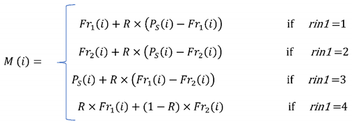
Equation (36) utilizes four distinct operators, and a random integer number between 1 and 4 (rin1) is generated to choose which operator is applied in the equation. This method introduces variability into the optimization process, enhancing the algorithm's ability to explore the search space and improving its convergence efficiency. Equation (35) outlines a discrete recombination process involving the new virion and a random number. Although this process aims to enhance diversity, it can unintentionally weaken the robustness of the original COVIDOA. Additionally, the performance of the original COVIDOA is highly sensitive to the mutation rate (MR), making it difficult to determine an optimal MR value for different optimization problems. To overcome these limitations, this paper introduces a hybrid recombination process as a replacement for the discrete recombination method used in the original COVIDOA. The hybrid recombination process is defined as follows:
By implementing the modifications outlined in Figure 2 of the flowchart, a robust version of the ENHCOVIDOA is developed, which is essential for effectively applying population-based algorithms to non-linear and non-convex problems. The ENHCOVIDOA demonstrates strong robustness, enabling it to effectively explore the complex and irregular search spaces commonly encountered in such optimization tasks. This leads to more consistent and precise results. By integrating this improved algorithmic design, COVIDOA becomes more capable of managing the complexities of DG uncertainty, ultimately enhancing system performance and efficiency.
5. Simulation Results and Discussion
The following thirteen cases were analyzed to evaluate the effectiveness of ENHCORONA with both IEEE (30&57) Bus system and Standard Iraq super grid high voltage (SISGHV- 28 Buses System)
5.1. The Analyzed Cases for the IEEE 30-Bus System
The IEEE 30-bus test system includes 6 generators, with bus 1 designated as the slack bus. It also comprises 24 load buses, 41 branches, 4 transformers, and 9 shunt reactive power injections, as outlined in Table 1. The optimization problem involves 24 control variables, with boundaries set between [0.94–1.06] for voltage magnitude, [0.9–1.1] for transformer tap settings, and [0–5 MVAr] for VAR compensators. Detailed line and bus data for the IEEE 30-bus system can be found in [22]. The system's active and reactive power demands are 283.4 MW and 126.2 MVAr, respectively. The IEEE 30-bus system has been updated to incorporate DG units based on renewable energy sources. The ideal placement of the DG unit is determined by analyzing of power flow of system [34]; for this case, bus number 30 was chosen. At this location, the DG unit's capacity is set at 5 MW, comprising 1 MW from solar cells and 4 MW from wind turbines. The study of the IEEE 30-bus system will include five cases. The first two cases (1&2) compare the performance of algorithms in identifying the MO-OPF without DG. The next two cases (3 & 4) focus on comparing algorithm performance in identifying MO-OPF with DG. The fifth case evaluates the MO-OPF using the TPEM-ENHCOVIDOA approach, considering the uncertainty associated with DG. The weight factors for all cases of IEEE-30 Bus in this study were chosen following [24], with values of = 21, = 22, and = 19, to maintain the balance among the different objectives of the problem.
- Case 1: Minimizing multi objectives of OPF the fuel cost, emissions, voltage deviation and losses without DG by COVIDOA.
- Case 2: Minimizing multi objectives of OPF the fuel cost, emissions, voltage deviation and losses without DG by ENHCOVIDOA .
- Case 3: Minimizing multi objectives of OPF the fuel cost, emissions, voltage deviation and losses with DG by COVIDOA.
- Case 4: Minimizing multi objectives of OPF the fuel cost, emissions, voltage deviation and losses with DG by ENHCOVIDOA .
- Case 5: Estimating multiple objectives, including fuel cost, emissions, voltage deviation, and losses under the uncertainty of DG by using TPEM & ENHCOVIDOA.
5.2. The Analyzed Cases for the IEEE 57-Bus System
This test system comprises 7 generators, with the reference generator positioned at bus 1, 50 load buses, 80 transmission lines, 17 transformers, and 3 capacitor banks to reactive power injections. It also includes six real power outputs from the generators, resulting in a total of 33 control variables for the OPF problem. The voltage magnitudes are limited between 0.94 and 1.06 per unit, while the transformer tap settings are restricted between 0.9 and 1.1 per unit. The range for reactive power compensation is from 0 to 20 MVAr. Specific details about the lines and buses can be found in [22]. The system's active power demand is 1250.8 MW, and the reactive power demand is 336.4 MVAr. In this study of the IEEE 57-bus system, the combined objective function uses weighting factors of 300 for , 30 for , and 600 for from [23]. Additionally, the IEEE 57-bus system has been enhanced by adding DG units [23]. The optimal locations for these DG units are identified as buses 35 and 36, with the solar unit having a capacity of 47.9067 MW and the wind unit having a capacity of 47.2636 MW. The study of the IEEE 57-bus system will include five cases. The first two cases (6 & 7) compare the performance of algorithms in identifying the MO-OPF without DG. The next two cases of IEEE 57-bus system (8 & 9) focus on comparing algorithm performance in identifying MO-OPF with DG. The tenth case evaluates the MO-OPF using the TPEM-ENHCOVIDOA approach, considering the uncertainty associated with DG.
- Case 6: Minimizing multi objectives of OPF the fuel cost, emissions, voltage deviation and losses without DG by COVIDOA.
- Case 7: Minimizing multi objectives of OPF the fuel cost, emissions, voltage deviation and losses without DG by ENH COVIDOA .
- Case 8: Minimizing multi objectives of OPF the fuel cost, emissions, voltage deviation and losses with DG by COVIDOA.
- Case 9 : Minimizing multi objectives of OPF the fuel cost, emissions, voltage deviation and losses with DG by ENHCOVIDOA .
- Case 10: Estimating multiple objectives, including fuel cost, emissions, voltage deviation, and losses under the uncertainty of DG by using TPEM & ENHCOVIDOA.
5.3. The Analyzed Cases for SISGHV-28 Buses System
The SISGHV-28 buses test system consists of 14 generators, with bus 1 serving as the slack bus. It also includes 14 load buses and 39 branches. The optimization problem is formulated with 27 control variables, where the voltage magnitude is constrained between [0.94–1.06] for the generator. Specific line and bus data for the SISGHV-28 buses system can be referenced in [22,35]. The system's active and reactive power demands are 5994.00 MW and 2657.00 MVAr, respectively. The SISGHV-28 buses system has been upgraded to integrate DG units based on renewable energy sources. The optimal placement of the DG units is determined through power flow analysis, identifying buses with the highest active and reactive power load and losses in the SISGHV-28 buses system. For this scenario, bus numbers 17 and 27 were selected, and the DG unit's total capacity is 300 MW, split between 100 MW from solar cells and 200 MW from wind turbines as 5% penetration of DG with power system. The weight factors for all cases of SISGHV-28 buses system in this study were chosen following [24], with values of = 21, = 22, and = 19, to maintain the balance among the different objectives of the problem. The study of the SISGHV-28 buses system will include three cases. The first one case (11) identifying the MO-OPF without DG by ENHCOVIDOA. The next case (12) focus on identifying MO-OPF with DG by ENHCOVIDOA. The last case (13) evaluates the MO-OPF using the TPEM-ENHCOVIDOA approach, considering the uncertainty associated with DG.
- Case 11 : Minimizing multi objectives of OPF the fuel cost, emissions, voltage deviation and losses without DG by ENH COVIDOA.
- Case 12 : Minimizing multi objectives of OPF the fuel cost, emissions, voltage deviation and losses with DG by ENH COVIDOA.
- Case 13 : Estimating multiple objectives, including fuel cost, emissions, voltage deviation, and losses under the uncertainty of DG by using TPEM & ENHCOVIDOA.
Several exams were performed with different population sizes and iteration counts. The best results, as discussed in this paper, were obtained with a population size of 50 and 200 iterations for the IEEE 30-bus test system in cases 1-4, and a population size of 50 with 300 iterations for the IEEE 57-bus test system in cases 6-9. These cases present the OPF results, both with and without DG, using COVIDOA and ENHCOVIDOA algorithms. For multi-objective estimation using TPEM, the optimal results were achieved with a population size of 50 and 100 iterations for the IEEE 30-bus test system in case 5, and a population size of 50 with 200 iterations for the IEEE 57-bus test system in case 10. In the reality application of the SISGHV-28 buses system, a population size of 50 and 200 iterations was used in cases 11 and 12. For case 13, using the TPEM method, the population size was 50 with 100 iterations. All algorithms were implemented in MATLAB 2020a, running on a 3.6 GHz Intel Core i7 processor with 8 GB RAM and a 64-bit operating system.
- Case (1&2) : IEEE 30-Bus System Minimizing multi objectives of OPF the fuel cost, emissions, voltage deviation and losses without DG by COVIDOA in case1& ENHCOVIDOA for case2 .
In cases 1 and 2 of the OPF problem, equation (18) was applied to the IEEE 30-bus system to determine the objectives of the OPF. The four objective functions were identified using the COVIDOA algorithm, as shown for case 1 in Table 1, and using the ENHCOVIDOA algorithm for case 2. These objectives are similar to those employed in algorithms such as MCOA [4], J-PPS3 [23], AGTLBO [24], and PSO-SSO [36]. This approach provides a systematic method for handling objective functions in OPF problems. In this study, for cases 1 and 2, both COVIDOA and ENHCOVIDOA were used to solve the OPF problem by optimizing a combined objective function. This function includes fuel cost, power loss, emissions, and voltage deviation, all evaluated without considering DG. Additionally, the results for active and reactive power, as well as voltage levels for generators, transformers, and capacitor banks, were maintained within the maximum and minimum limits of the IEEE 30-bus system. And compatible with optimal control variable settings are detailed in Table 1, for these cases. Table 2, provides a comparison of the results obtained from the proposed algorithms with those from recent studies. The results from COVIDOA align closely with those reported in the literature. However, the enhanced ENHCOVIDOA algorithm demonstrates superior performance in optimizing multiple objectives, including fuel cost, power loss, emissions, and voltage deviation. The effectiveness of ENHCOVIDOA is further validated by its convergence to a combined objective function value of 936.5081 $/h, compared to COVIDOA's 938.1275 $/h, as illustrated in Figure 3 (a & b). Moreover, Figures 4 (a & b). depict the voltage profiles obtained from the COVIDOA and ENHCOVIDOA , confirming that the voltage levels at all buses remained within the specified upper and lower limits.
- Case (3&4): IEEE 30-Bus System Minimizing multi objectivesof OPF the fuel cost, emissions, voltage deviation and losses with DG by COVIDOA in case3& ENHCOVIDOA for case4.
The inclusion of DG was found to enhance the results, outperforming the outcomes of Cases (1 & 2). Specifically, the combined objective function value using COVIDOA dropped from 938.1275 $/h in Case 1 to 925.0389 $/h in Case 3. Similarly, with ENHCOVIDOA, the value decreased from 936.5081 $/h in Case 2 to 922.4154 $/h in Case 4, representing a 1.3951% reduction in the combined objective function for COVIDOA, saving 13.0886 $ per hour, and a 1.5048% reduction for ENHCOVIDOA, resulting in a 14.0927 $ hourly saving. The results, including optimal control variable settings for COVIDOA and ENHCOVIDOA, were compared with those of the DA, GWO, Jaya, J-PPS1, J-PPS2, and J-PPS3 algorithms from [23]. as shown in Table 3. The ENHCOVIDOA, an Evolutionary Computing-based approach, demonstrated superior performance in handling the OPF problem in large-scale systems with DG units. The convergence characteristics of COVIDOA and ENHCOVIDOA after DG integration are depicted in Figure 5 (a &b) respectively, while Figure 6 a and b confirm that voltage magnitudes across all buses remain within the specified limits in both Cases (3 &4).
- Case 5: IEEE 30-Bus System Estimating multiple objectives, including fuel cost, emissions, voltage deviation, and losses under the uncertainty of DG by using TPEM-ENHCOVIDOA
As shown in Table 1, the ENHCOVIDOA in Case 4 resulted in a fuel cost of $810.12 per hour. In Case 5, the TPEM-ENHCOVIDOA demonstrated higher accuracy, achieving a greater reduction in fuel cost, lowering it to $799.9597 as mean value, accounting for the uncertainties of wind and solar energy as DG across six scenarios , as noted in Tables (1& 4). This represents a 1.2540% decrease, equivalent to a savings of $10.1589 per hour. This reduction amounts to a total saving of $243.8137 per day, $7314.4114 per month, and $87,772.9374 annually compared to the multi-objective results in Case 4. Additionally, the standard deviations for all objectives listed in Table 4 are 26.1802 for fuel cost, 0.2207for power loss, 0.00551for emissions, and 0.08106for voltage deviation. These low values indicate greater confidence in the estimates, with the results closely aligning with the mean values. Moreover, as shown in Figure 7, the computational effort was reduced, resulting in faster convergence.
- Case (6&7): IEEE 57-Bus System Minimizing multi objectives of OPF the fuel cost, emissions, voltage deviation and losses without DG by COVIDOA in case 6 & ENHCOVIDOA for case7 .
To evaluate the scalability and efficiency of the COVIDOA and ENHCOVIDOA algorithms in solving large-scale problems, they were applied to the OPF problem on the IEEE 57-bus test system without DG for cases 6 and 7. The results for active and reactive power, as well as voltage levels for generators, transformers, and capacitor banks, were maintained within the maximum and minimum limits of the IEEE 57-bus system and compatible to optimal control variable settings are detailed in Table 1 for these cases. Additionally, the objective function for the OPF in these cases includes fuel cost, emissions, real power loss, and total voltage deviation, as shown in Table 5. The performance of COVIDOA and ENHCOVIDOA, along with their optimal control variable settings, was compared to other algorithms from the literature, such as DA, GWO, Jaya, J-PPS1, J-PPS2, TLBO, and AGTLBO, as presented in Table 6. The ENHCOVIDOA algorithm demonstrated superior performance in addressing the multi-objective OPF problem (fuel cost, power loss, emissions, and voltage deviation) for a large-scale power system. COVIDOA and ENHCOVIDOA achieved combined objective function values of $42,487.3796/h and $42,417.1976/h, respectively, with ENHCOVIDOA converging faster than COVIDOA. This indicates that ENHCOVIDOA outperformed COVIDOA in cases 6 and 7 without violating any constraints, as illustrated in Figure 8 (a & b). Additionally, the bus voltage profiles obtained from both algorithms remained within the specified limits, as shown in Figure 9 (a & b).
- Case (8 & 9): IEEE 57-Bus System Minimizing multi objectives of OPF the fuel cost, emissions, voltage deviation and losses with DG by COVIDOA in case 8 &ENHCOVIDOA for case9 .
In these cases, the performance of COVIDOA and ENHCOVIDOA in solving the OPF problem was assessed using the IEEE 57-bus test system, incorporating two DGs. The results, along with the optimal control variable settings obtained by ENHCOVIDOA, were compared with those of other algorithms, including DA, GWO, Jaya, J-PPS1, J-PPS2, and J-PPS3 from prior research , as well as with COVIDOA (without enhancements) from our study, as shown in Table 7. This comparison highlights the superior performance of ENHCOVIDOA in handling multiple objectives, such as fuel cost, emissions, real power loss, and total voltage deviation. The proposed ENHCOVIDOA algorithm achieved a combined objective function value of 38,733.676, outperforming other methods while satisfying all constraints. The combined objective function value of ENHCOVIDOA improved by 8.68%, decreasing from 42,417.1976 in Case 7 to 38,733.676 in Case 9 after the inclusion of two DGs, as expected.
- Case 10 : IEEE 57-Bus System Estimatingmultiple objectives, including fuel cost, emissions, voltage deviation, and losses under the uncertainty of DG by using TPEM & ENHCOVIDOA
As shown in Table 5, the ENHCOVIDOA method in Case 9 resulted in a fuel cost of $37,799 per hour. In Case 10, the TPEM-ENHCOVIDOA demonstrated higher accuracy, achieving a greater reduction in fuel cost, lowering it to $37,753.71 per hour as mean value, accounting for the uncertainties of wind and solar energy as DG across six scenarios. This suggests that the TPEM-ENHCOVIDOA approach in Case 10 produced more precise results, leading to a 0.1198% reduction in fuel costs, equivalent to savings of $45.28 per hour. These savings total $1,086.80 per day, $32,603.91 per month, and $391,246.87 annually when compared to the ENHCOVIDOA method in Case 9. Additionally, the standard deviations for all objectives listed in Table 8 are 1175.8062 for fuel cost, 1.2534 for power loss, 0.0668 for emissions, and 0.06986 for voltage deviation. These low values indicate greater confidence in the estimates, with the results closely aligning with the mean values. Moreover, as shown in Figure 10, the computational effort was reduced, resulting in faster convergence.
- Cases (11,12&13) : SISGHV-28 buses systemEstimating multiple objectives, including fuel cost, emissions, voltage deviation, and losses under the uncertainty of DG by using TPEM & ENHCOVIDOA.
In Case 11, as detailed in Table 9, the OPF of the SISGHV-28 buses system was evaluated while considering the system's control variable values. This case also explored the multi-objective optimization of OPF using the ENHCOVIDOA method without DG. In Table 10, the ENHCOVIDOA method in Case 12 resulted in an average fuel cost of $24,053.64 per hour, accounting for the uncertainties of wind and solar energy as DG across six scenarios. In contrast, the TPEM method integrated with ENHCOVIDOA achieved a lower fuel cost of $23,762.34 per hour. This indicates that the TPEM-ENHCOVIDOA approach in Case 13 yielded more accurate results, resulting in a 1.2% reduction in fuel costs, which translates to savings of $288.64 per hour. Over time, these savings add up to $ 6,927.45 daily, $ 207,823.45 monthly, and $ 2,493,881.40 annually when compared to Case 12 with ENHCOVIDOA alone. Moreover, the standard deviations for all objectives listed in Table 10—896.08 for fuel cost, 0.91397 for emissions, and 0.01563 for voltage deviation are relatively low, reflecting higher confidence in the estimates and indicating that the results are closely aligned with the mean values. However, the standard deviation for power loss was recorded at 7.6639, indicating increased variability in power loss across the seven scenarios. Nonetheless, the power loss values, within ±7.6639, remain acceptable when compared to findings from other studies, such as [22] and [35].
6. Conclusion
This paper presents a multi-objective adaptation of the recently introduced COVIDOA algorithm, referred to as ENHCOVIDOA, aimed at solving optimization challenges like optimal power flow while considering four objectives: cost, power loss, emissions, and voltage deviation. ENHCOVIDOA preserves the core search strategy of COVIDOA, integrating an archiving system and a selection process. The evaluation of solutions in ENHCOVIDOA is performed using a weighted approach with co-scaling coefficients. To validate its effectiveness, the proposed algorithm was applied to two IEEE test systems (30,57 ) Buses and reality system from Iraq SISGHV- 28 Buses under various cases, leading to the following key conclusions:
- The ENHCOVIDOA enhances search ability in high-dimensional problems like multi-objective of OPF. In case 1&2 of the IEEE 30-Bus and case 6&7 of the IEEE 57 system, ENHCOVIDOA reduces fuel cost, emissions, and voltage deviation for 30 Bus by (0.5258%, 1.7966%, and 12.1419%) and for 57 Bus by (0.1643%, 0.0641%, and 0.9715%) when compared to the original COVIDOA without present DG.
- The effectiveness of the proposed ENHCOVIDOA method, enhanced for optimizing multi-objective OPF problems, particularly in the presence of renewable energy generation such as wind and solar as DG is certainty. As highlighted by the results, significant reductions in fuel cost, emissions, and voltage deviation were achieved. For the IEEE 30 Bus system, in cases (3&4) these reductions were 0.3076%, 2.5168%, and 6.0630% respectively, while for the IEEE 57 Bus system, in cases (8 & 9) the reductions were 0.1400%, 0.2667%, and 1.7734%, respectively, when compared to the results of the COVIDOA method. Moreover, ENHCOVIDOA outperforms other algorithms from the literature, as demonstrated by the data presented in the tables.
- In cases 5 and 10, a new methodology was introduced to solve the MOPF problem under uncertain renewable generation using the TPEM. The results highlight the superior performance of the TPEM-ENHCOVIDOA, providing greater accuracy and more optimal outcomes. This led to significant annual fuel cost savings, with $87,772.94 for the IEEE 30 Bus system and $391,246.87 for the IEEE 57 Bus system, compared to cases 4 and 9, which did not incorporate TPEM.
- In Cases 12 and 13, the effectiveness of the proposed TPEM-ENHCOVIDOA method was tested using a reality system from Iraq's SISGHV-28 Buses, both with and without DG. The method successfully optimized multiple objectives, resulting in annual fuel cost savings of $2,493,881.40.
- Based on the presented information, the algorithm is also scalable for larger systems and has shown competitive performance, as evidenced by the results.
Author Contributions
Conceptualization, B A.-B. and O.K.; methodology, B A.-B.; software, B A.-B.; validation, B A.-B., and O.K. ; formal analysis, B A.-B.; investigation, B A.-B. and O.K.; data curation, B A.-B.; writing—original draft preparation, B A.-B.; writing—review and editing, O.K. ; visualization, B A.-B. and O.K.; supervision, O.K.; project administration, O.K.; funding acquisition, O.K. All authors have read and agreed to the published version of the manuscript.
Funding
This research received no external funding.
Data Availability Statement
Not applicable.
| Abbreviations and Acronyms | Description |
| Selected objective function | |
| Total no. of objective functions | |
| Equality constraints | |
| Inequality constraints | |
| a and b | The state and control variable. |
| Apparent power flow of transmission line | |
| The total generation cost function | |
| The total emission functions | |
| Active and reactive power output generation | |
| The demand for active and reactive power at the load bus | |
| The total voltage deviation function | |
| The voltage magnitude of generation | |
| The voltage magnitude for bus | |
| Voltage reference equal to 1.0 per unit | |
| The voltage magnitude for transmission line | |
| Cost coefficients of the th generator | |
| Emission coefficients | |
| Reactive power of the VAR source | |
| COVIDOA | Coronavirus Disease Optimization Algorithm |
| ENHCOVIDOA | Enhanced Coronavirus Disease Optimization Algorithm |
| COA | Cuckoo optimization algorithm |
| MCOA | The modified Cuckoo optimization algorithm |
| TFWO | Turbulent flow of a water-based optimizer |
| SMA | SlimeMould Algorithm |
| J-PPS | Jaya algorithm and Powell’s Pattern Search |
| Jaya | Jaya algorithm |
| TLBO | Teaching–learning-based optimization |
| AGTLBO | Adaptive Gaussian Teaching–learning-based optimization |
| HHO | Harris Hawks Optimization |
| PSO-SSO | Particle swarm optimization with slap swarm optimization |
| DA | Dragonfly Algorithm |
| GWO | Grey Wolf Optimization |
| MODA | Multi-objective dragon fly |
| MOICA | Multi-objective imperialist competitive algorithm |
| MOMICA | Multi-Objective Modified Imperialist Competitive Algorith |
Appendix A
Coefficient Generating Unit

Table A1.
The cost and emission coefficients of generators for the IEEE 30-bus test system.
| Fuel cost coefficient | |||||||
|---|---|---|---|---|---|---|---|
| G1 | G2 | G5 | G8 | G11 | G13 | ||
| a | 0.00375 | 0.0175 | 0.0625 | 0.00834 | 0.025 | 0.025 | |
| b | 2 | 1.75 | 1 | 3.25 | 3 | 3 | |
| c | 0 | 0 | 0 | 0 | 0 | 0 | |
| Emission coefficient | |||||||
| 4.091 | 2.543 | 4.258 | 5.326 | 4.258 | 6.131 | ||
| -5.554 | -6.047 | -5.094 | -3.55 | -5.094 | -5.555 | ||
| 6.49 | 5.638 | 4.586 | 3.38 | 4.586 | 5.151 | ||
| 2.00 | 5.00 | 1.00 | 2.00 | 1.00 | 1.00 | ||
| 2.857 | 3.33 | 8 | 2 | 8 | 6.67 | ||
Table A2.
The cost and emission coefficients of generators for the IEEE 57-bus test system.
| Fuel cost coefficient | |||||||
|---|---|---|---|---|---|---|---|
| G1 | G2 | G3 | G6 | G8 | G9 | G12 | |
| a | 0.0775795 | 0.01 | 0.25 | 0.01 | 0.0222222222 | 0.01 | 0.0322580645 |
| b | 20 | 40 | 20 | 40 | 20 | 40 | 20 |
| c | 0 | 0 | 0 | 0 | 0 | 0 | 0 |
| Emission coefficient | |||||||
| 4.091 | 2.543 | 6.131 | 3.491 | 4.258 | 2.754 | 5.326 | |
| -5.554 | -6.047 | -5.555 | -5.754 | -5.094 | -5.847 | -3.555 | |
| 6.49 | 5.638 | 5.151 | 6.39 | 4.586 | 5.238 | 3.38 | |
| 2.00 | 5.00 | 1.00 | 3.00 | 1.00 | 4.00 | 0.002 | |
| 0.286 | 0.333 | 0.667 | 0.266 | 0.8 | 0.288 | 0.2 | |
Table A3.
The generator cost coefficients for the SISGHV network.
| Generator | a | b | c | |
| 1 | 275 | 0.35 | 0.0012 | |
| 2 | 0 | 0 | 0 | |
| 3 | 200 | 3.5 | 0.04 | |
| 4 | 2581 | 2.155 | 0.05 | |
| 5 | 1698 | 11.91 | 0.03 | |
| 6 | 154 | 7.05 | 0.0136 | |
| 7 | 200 | 0.64 | 0.0017 | |
| 8 | 0 | 0 | 0 | |
| 9 | 250 | 0.5 | 0.02 | |
| 10 | 300 | 2.2 | 0.003 | |
| 11 12 13 14 |
200 159 120 685 |
0.652 0.561 0.8 3.1 |
0.002 0.002 0.0025 0.0158 |
Table A4.
The generator emission coefficients for the SISGHV network.
| Generator | |||||
| 1 | 2.543 | -6.047 | 5.638 | 0.00005 | 0.5047 |
| 2 | 4.091 | -5.554 | 6.490 | 0.00042 | 0.000288 |
| 3 | 3.123 | -6.085 | 5.643 | 0.0003 | 0.376 |
| 4 | 3.642 | -3.441 | 3.564 | 0.0001 | 0.045 |
| 5 | 4.785 | -1.765 | 3.432 | 0.0002 | 0.287 |
| 6 | 3.765 | -5.333 | 6.543 | 0.00065 | 0.34 |
| 7 | 3.456 | -3.567 | 4.485 | 0.000032 | 0.0076 |
| 8 | 2.473 | -2.084 | 3.538 | 0.000132 | 0.043 |
| 9 | 3.258 | -2.084 | 6.566 | 0.000002 | 0.054 |
| 10 | 1.416 | -6.510 | 2.310 | 0.0001 | 0.68 |
| 11 12 13 14 |
3.255 4.221 2.198 6.456 |
-5.064 -6.333 -4.542 -4.441 |
3.555 3.231 1.586 3.131 |
0.0005 0.000014 0.0004 0.00001 |
0.098 0.57 0.012 0.266 |
Table A5.
Data of Buses of SISGHV.
| Bus | Voltage Mag(pu) | Voltage Ang(deg) | Generation P (MW) |
Generation Q (MVAr) |
Load P (MW) |
Load Q (MVAr) |
| 1 | 1.039 | 0.000 | 159.40 | 2347.40 | 206.00 | 56.00 |
| 2 | 1.020 | 9.525 | 396.59 | 77.77 | - | - |
| 3 | 1.010 | 7.695 | 282.29 | -46.24 | 150.00 | 75.00 |
| 4 | 1.020 | 6.74 | 347.61 | -84.12 | 125.00 | 93.00 |
| 5 | 1.020 | 6.792 | -0.00 | -25.51 | - | - |
| 6 | 1.020 | -0.773 | 247.07 | -112.80 | 130.00 | 10.00 |
| 7 | 1.010 | 2.645 | 1390.76 | 162.09 | - | - |
| 8 | 1.020 | 0.243 | 382.55 | -75.50 | 200.00 | 50.00 |
| 9 | 1.020 | -0.654 | 564.91 | -1946.89 | - | - |
| 10 | 1.030 | 1.618 | 351.72 | 34.22 | - | - |
| 11 | 1.030 | -2.117 | 266.86 | -77.00 | - | - |
| 12 | 1.020 | -9.663 | 572.14 | -85.11 | 423.00 | 101.00 |
| 13 | 1.010 | -9.48 | 605.83 | 78.51 | 155.00 | 72.00 |
| 14 | 1.010 | 7.252 | 445.07 | 48.50 | 200.00 | 101.00 |
| 15 | 1.011 | -1.251 | - | - | 650.00 | 302.00 |
| 16 | 1.020 | -0.947 | - | - | - | - |
| 17 | 1.004 | -1.802 | - | - | 576.00 | 302.00 |
| 18 | 1.006 | -1.583 | - | - | 849.00 | 295.00 |
| 19 | 1.008 | -0.533 | - | - | 413.00 | 149.00 |
| 20 | 1.014 | -1.278 | - | - | 127.00 | 56.00 |
| 21 | 1.005 | -1.528 | - | - | 50.00 | 182.00 |
| 22 | 1.004 | -1.953 | - | - | 84.00 | 22.0 |
| 23 | 1.022 | -2.023 | - | - | 260.00 | 108.00 |
| 24 | 1.016 | -1.438 | - | - | 109.00 | 40.00 |
| 25 | 1.032 | -0.650 | - | - | 308.00 | 185.00 |
| 26 | 1.026 | -1.080 | - | - | 213.00 | 152.00 |
| 27 | 0.998 | -3.604 | - | - | 311.00 | 161.00 |
| 28 | 1.005 | -0.693 | - | - | 455.00 | 145.00 |
Table A6.
Power flow parameter data for the lines of SISGHV.
| Branch # | From Bus |
To Bus |
From Bus P (MW) |
Injection Q (MVAr) |
To Bus P (MW) |
Injection Q (MVAr) |
Loss P (MW) |
Loss Q (MVAr) |
| 1 | 15 | 2 | -197.71 | -71.63 | 198.3 | 38.88 | 0.591 | 4.83 |
| 2 | 15 | 3 | -135.63 | -3.22 | 135.95 | -42.66 | 0.328 | 2.98 |
| 3 | 15 | 4 | -67.7 | -72.53 | 67.91 | -35.55 | 0.202 | 1.65 |
| 4 | 15 | 6 | -51.26 | -82.99 | 51.4 | -54.16 | 0.138 | 1.26 |
| 5 | 3 | 4 | -3.67 | -78.58 | 3.7 | -12.49 | 0.036 | 0.33 |
| 6 | 4 | 5 | 0 | -0.3 | 0 | -0.3 | 0 | 0 |
| 7 | 4 | 17 | 76.5 | -38.96 | -76.19 | -91.6 | 0.31 | 2.82 |
| 8 | 4 | 17 | 74.5 | -41.54 | -74.2 | -92.68 | 0.302 | 2.75 |
| 9 | 4 | 8 | 0 | -48.28 | 0 | -48.28 | 0 | 0 |
| 10 | 5 | 6 | 0 | -25.2 | 0 | -25.2 | 0 | 0 |
| 11 | 6 | 18 | 65.67 | -43.44 | -65.44 | -91.23 | 0.238 | 2.16 |
| 12 | 17 | 19 | -265.57 | -20.68 | 266.22 | 1.2 | 0.651 | 5.93 |
| 13 | 17 | 21 | -87.11 | -3.61 | 87.16 | -12.47 | 0.046 | 0.42 |
| 14 | 17 | 8 | -72.92 | -93.42 | 73.22 | -43.24 | 0.297 | 2.7 |
| 15 | 16 | 20 | 87.13 | 55 | -87.04 | -77.06 | 0.095 | 0.87 |
| 16 | 16 | 20 | 87.13 | 55 | -87.04 | -77.06 | 0.095 | 0.87 |
| 17 | 16 | 21 | 137.57 | 146.94 | -137.16 | -169.53 | 0.409 | 3.72 |
| 18 | 16 | 1 | -131.66 | -196.05 | 132.24 | 167.09 | 0.581 | 4.84 |
| 19 | 16 | 9 | -186.35 | 4.86 | 186.72 | -31.55 | 0.37 | 3.08 |
| 20 | 16 | 26 | 6.18 | -65.74 | -6.17 | -20.74 | 0.016 | 0.15 |
| 21 | 18 | 19 | -708.65 | -1.8 | 710.09 | 6.94 | 1.44 | 13.01 |
| 22 | 18 | 20 | -158.98 | -200.96 | 159.25 | 191.52 | 0.269 | 2.47 |
| 23 | 18 | 22 | 84.06 | -1.02 | -84 | -22 | 0.062 | 0.56 |
| 24 | 19 | 7 | -694.66 | -78.57 | 695.38 | 81.04 | 0.721 | 6.63 |
| 25 | 19 | 7 | -694.66 | -78.57 | 695.38 | 81.04 | 0.721 | 6.63 |
| 26 | 20 | 10 | -112.17 | -93.39 | 112.56 | 28.56 | 0.381 | 3.47 |
| 27 | 23 | 10 | -238.22 | -46.18 | 239.17 | 5.66 | 0.95 | 8.64 |
| 28 | 23 | 12 | -91.85 | -43.94 | 92.21 | -74.11 | 0.361 | 3.28 |
| 29 | 23 | 27 | 70.06 | -17.89 | -69.73 | -110.64 | 0.337 | 3.07 |
| 30 | 8 | 24 | 109.34 | -33.98 | -109 | -40 | 0.336 | 2.75 |
| 31 | 1 | 9 | -373.62 | 1950.02 | 378.19 | -1915.35 | 4.572 | 38.15 |
| 32 | 1 | 25 | 97.39 | 87.15 | -97.24 | -108.65 | 0.144 | 1.2 |
| 33 | 1 | 25 | 97.39 | 87.15 | -97.24 | -108.65 | 0.144 | 1.2 |
| 34 | 25 | 11 | -157.98 | 36.08 | 158.21 | -58.33 | 0.23 | 1.89 |
| 35 | 25 | 26 | 44.47 | -3.79 | -44.41 | -60.08 | 0.061 | 0.51 |
| 36 | 11 | 26 | 108.65 | -18.68 | -108.39 | -40 | 0.255 | 2.09 |
| 37 | 26 | 12 | -54.03 | -31.19 | 54.16 | -75.69 | 0.126 | 1.14 |
| 38 | 12 | 14 | 2.77 | -36.31 | -2.75 | -85.34 | 0.027 | 0.25 |
| 39 | 27 | 13 | -241.27 | -50.36 | 242.97 | -13.02 | 1.699 | 15.47 |
References
- U. Khan, N. Javaid, K. A. A. Gamage, C. James Taylor, S. Baig, and X. Ma, “Heuristic Algorithm Based Optimal Power Flow Model Incorporating Stochastic Renewable Energy Sources,” IEEE Access, vol. 8, pp. 148622–148643, 2020. [CrossRef]
- M. H. Nadimi-Shahraki, S. Taghian, S. Mirjalili, L. Abualigah, M. A. Elaziz, and D. Oliva, “Ewoa-opf: Effective whale optimization algorithm to solve optimal power flow problem,” Electronics (Switzerland), vol. 10, no. 23, Dec. 2021. [CrossRef]
- Adhikari, F. Jurado, S. Naetiladdanon, A. Sangswang, S. Kamel, and M. Ebeed, “Stochastic optimal power flow analysis of power system with renewable energy sources using Adaptive Lightning Attachment Procedure Optimizer,” International Journal of Electrical Power and Energy Systems, vol. 153, Nov. 2023. [CrossRef]
- Alanazi, “Optimal Power Flow Considering Solar and Wind Energy Systems Via Modified Cuckoo Optimization Algorithm,” Journal of the North for Basic and Applied Sciences, no. 8, 2023. [CrossRef]
- S. Alghamdi, “Optimal Power Flow of Renewable-Integrated Power Systems Using a Gaussian Bare-Bones Levy-Flight Firefly Algorithm,” Front Energy Res, vol. 10, May 2022. [CrossRef]
- T. H. B. Huy, D. Kim, and D. N. Vo, “Multiobjective Optimal Power Flow Using Multiobjective Search Group Algorithm,” IEEE Access, vol. 10, pp. 77837–77856, 2022. [CrossRef]
- S. Gupta, N. Kumar, L. Srivastava, H. Malik, A. Anvari-moghaddam, and F. P. García Márquez, “A robust optimization approach for optimal power flow solutions using rao algorithms,” Energies (Basel), vol. 14, no. 17, Sep. 2021. [CrossRef]
- S. Chandrasekaran, “Multiobjective optimal power flow using interior search algorithm: A case study on a real-time electrical network,” Comput Intell, vol. 36, no. 3, pp. 1078–1096, Aug. 2020. [CrossRef]
- F. Daqaq, M. Ouassaid, and R. Ellaia, “A new meta-heuristic programming for multi-objective optimal power flow,” Electrical Engineering, vol. 103, no. 2, pp. 1217–1237, Apr. 2021. [CrossRef]
- E. Naderi, M. Pourakbari-Kasmaei, F. V. Cerna, and M. Lehtonen, “A novel hybrid self-adaptive heuristic algorithm to handle single- and multi-objective optimal power flow problems,” International Journal of Electrical Power and Energy Systems, vol. 125, Feb. 2021. [CrossRef]
- M. Khalid, H. M. Hamza, S. Mirjalili, and K. M. Hosny, “MOCOVIDOA: a novel multi-objective coronavirus disease optimization algorithm for solving multi-objective optimization problems,” Neural Comput Appl, vol. 35, no. 23, pp. 17319–17347, Aug. 2023. [CrossRef]
- M. Khalid, K. M. Hosny, and S. Mirjalili, “COVIDOA: a novel evolutionary optimization algorithm based on coronavirus disease replication lifecycle,” Neural Comput Appl, vol. 34, no. 24, pp. 22465–22492, Dec. 2022. [CrossRef]
- L. A. Gallego, J. F. Franco, and L. G. Cordero, “A fast-specialized point estimate method for the probabilistic optimal power flow in distribution systems with renewable distributed generation,” International Journal of Electrical Power and Energy Systems, vol. 131, Oct. 2021. [CrossRef]
- F. Zishan, E. Akbari, and O. D. Montoya, “Analysis of probabilistic optimal power flow in the power system with the presence of microgrid correlation coefficients,” Cogent Eng, vol. 11, no. 1, 2023. [CrossRef]
- Bhattacharya, P. Das, and A. K. Chakraborty, “A novel approach towards uncertainty modeling in multiobjective optimal power flow with renewable integration,” International Transactions on Electrical Energy Systems, vol. 29, no. 12, Dec. 2019. [CrossRef]
- Ali, G. Abbas, M. U. Keerio, M. A. Koondhar, K. Chandni, and S. Mirsaeidi, “Solution of constrained mixed-integer multi-objective optimal power flow problem considering the hybrid multi-objective evolutionary algorithm,” IET Generation, Transmission and Distribution, vol. 17, no. 1, pp. 66–90, Jan. 2023. [CrossRef]
- M. Aien, M. Fotuhi-Firuzabad, and M. Rashidinejad, “Probabilistic optimal power flow in correlated hybrid wind-photovoltaic power systems,” IEEE Trans Smart Grid, vol. 5, no. 1, pp. 130–138, Jan. 2014. [CrossRef]
- M. Aien, R. Ramezani, and S. M. Ghavami, “Probabilistic Load Flow Considering Wind Generation Uncertainty,” 2011. [Online]. Available: www.etasr.com.
- M. Dadkhah and B. Venkatesh, “Cumulant based stochastic reactive power planning method for distribution systems with wind generators,” IEEE Transactions on Power Systems, vol. 27, no. 4, pp. 2351–2359, 2012. [CrossRef]
- K. Aurangzeb, S. Shafiq, M. Alhussein, Pamir, N. Javaid, and M. Imran, “An effective solution to the optimal power flow problem using meta-heuristic algorithms,” Front Energy Res, vol. 11, 2023. [CrossRef]
- S. Sarhan, R. El-Sehiemy, A. Abaza, and M. Gafar, “Turbulent Flow of Water-Based Optimization for Solving Multi-Objective Technical and Economic Aspects of Optimal Power Flow Problems,” Mathematics, vol. 10, no. 12, Jun. 2022. [CrossRef]
- M. Al-Kaabi, V. Dumbrava, and M. Eremia, “A Slime Mould Algorithm Programming for Solving Single and Multi-Objective Optimal Power Flow Problems with Pareto Front Approach: A Case Study of the Iraqi Super Grid High Voltage,” Energies (Basel), vol. 15, no. 20, Oct. 2022. [CrossRef]
- S. Gupta, N. Kumar, L. Srivastava, H. Malik, A. Pliego Marugán, and F. P. García Márquez, “A hybrid jaya–powell’s pattern search algorithm for multi-objective optimal power flow incorporating distributed generation,” Energies (Basel), vol. 14, no. 10, May 2021. [CrossRef]
- Alanazi, M. Alanazi, Z. A. Memon, and A. Mosavi, “Determining Optimal Power Flow Solutions Using New Adaptive Gaussian TLBO Method,” Applied Sciences (Switzerland), vol. 12, no. 16, Aug. 2022. [CrossRef]
- J. Zhao, L. Li, J. Yu, and Z. Li, “An Improved Marine Predators Algorithm for Optimal Reactive Power Dispatch With Load and Wind-Solar Power Uncertainties,” IEEE Access, vol. 10, pp. 126664–126673, 2022. [CrossRef]
- M. Ebeed, A. Alhejji, S. Kamel, and F. Jurado, “Solving the optimal reactive power dispatch using marine predators algorithm considering the uncertainties in load and wind-solar generation systems,” Energies (Basel), vol. 13, no. 17, Sep. 2020. [CrossRef]
- N. Karthik, A. K. Parvathy, R. Arul, and K. Padmanathan, “Multi-objective optimal power flow using a new heuristic optimization algorithm with the incorporation of renewable energy sources,” International Journal of Energy and Environmental Engineering, vol. 12, no. 4, pp. 641–678, Dec. 2021. [CrossRef]
- M. A. Ilyas, G. Abbas, T. Alquthami, M. Awais, and M. B. Rasheed, “Multi-Objective Optimal Power Flow with Integration of Renewable Energy Sources Using Fuzzy Membership Function,” IEEE Access, vol. 8, pp. 143185–143200, 2020. [CrossRef]
- S. M. Mohseni-Bonab, A. Rabiee, B. Mohammadi-Ivatloo, S. Jalilzadeh, and S. Nojavan, “A two-point estimate method for uncertainty modeling in multi-objective optimal reactive power dispatch problem,” International Journal of Electrical Power and Energy Systems, vol. 75, pp. 194–204, Feb. 2016. [CrossRef]
- J. M. Morales and J. Pérez-Ruiz, “Point estimate schemes to solve the probabilistic power flow,” IEEE Transactions on Power Systems, vol. 22, no. 4, pp. 1594–1601, 2007. [CrossRef]
- M. Peik-Herfeh, H. Seifi, and M. K. Sheikh-El-Eslami, “Decision making of a virtual power plant under uncertainties for bidding in a day-ahead market using point estimate method,” International Journal of Electrical Power and Energy Systems, vol. 44, no. 1, pp. 88–98, Jan. 2013. [CrossRef]
- Ramos-Figueroa, R. Kharel, M. Quiroz-Castellanos, and E. Mezura-Montes, “Variation Operators for Grouping Genetic Algorithms: A Review”. [CrossRef]
- G. Gad, “Particle Swarm Optimization Algorithm and Its Applications: A Systematic Review,” Archives of Computational Methods in Engineering, vol. 29, no. 5, pp. 2531–2561, Aug. 2022. [CrossRef]
- M. Z. Islam et al., “A Harris Hawks optimization based singleand multi-objective optimal power flow considering environmental emission,” Sustainability (Switzerland), vol. 12, no. 13, Jul. 2020. [CrossRef]
- M. AL-Kaabi, S. Q. Salih, A. I. B. Hussein, V. Dumbrava, and M. Eremia, “Optimal Power Flow Based on Grey Wolf Optimizer: Case Study Iraqi Super Grid High Voltage 400 kV,” in Lecture Notes in Networks and Systems, Springer Science and Business Media Deutschland GmbH, 2023, pp. 490–503. [CrossRef]
- L. Slimani and T. Bouktir, “Multi-objective optimal power flow considering the fuel cost, emission, voltage deviation and power losses using Multi-Objective Dragonfly algorithm,” 2017. [Online]. Available online: https://www.researchgate.net/publication/322939107.
- R. A. El Sehiemy, F. Selim, B. Bentouati, and M. A. Abido, “A novel multi-objective hybrid particle swarm and salp optimization algorithm for technical-economical-environmental operation in power systems,” Energy, vol. 193, Feb. 2020. [CrossRef]
- M. Ghasemi, S. Ghavidel, M. M. Ghanbarian, M. Gharibzadeh, and A. Azizi Vahed, “Multi-objective optimal power flow considering the cost, emission, voltage deviation and power losses using multi-objective modified imperialist competitive algorithm,” Energy, vol. 78, pp. 276–289, Dec. 2014. [CrossRef]
Figure 1.
flowchart of using TPEM for providing deterministic scenarios and estimating the uncertainty output variable.
Figure 1.
flowchart of using TPEM for providing deterministic scenarios and estimating the uncertainty output variable.
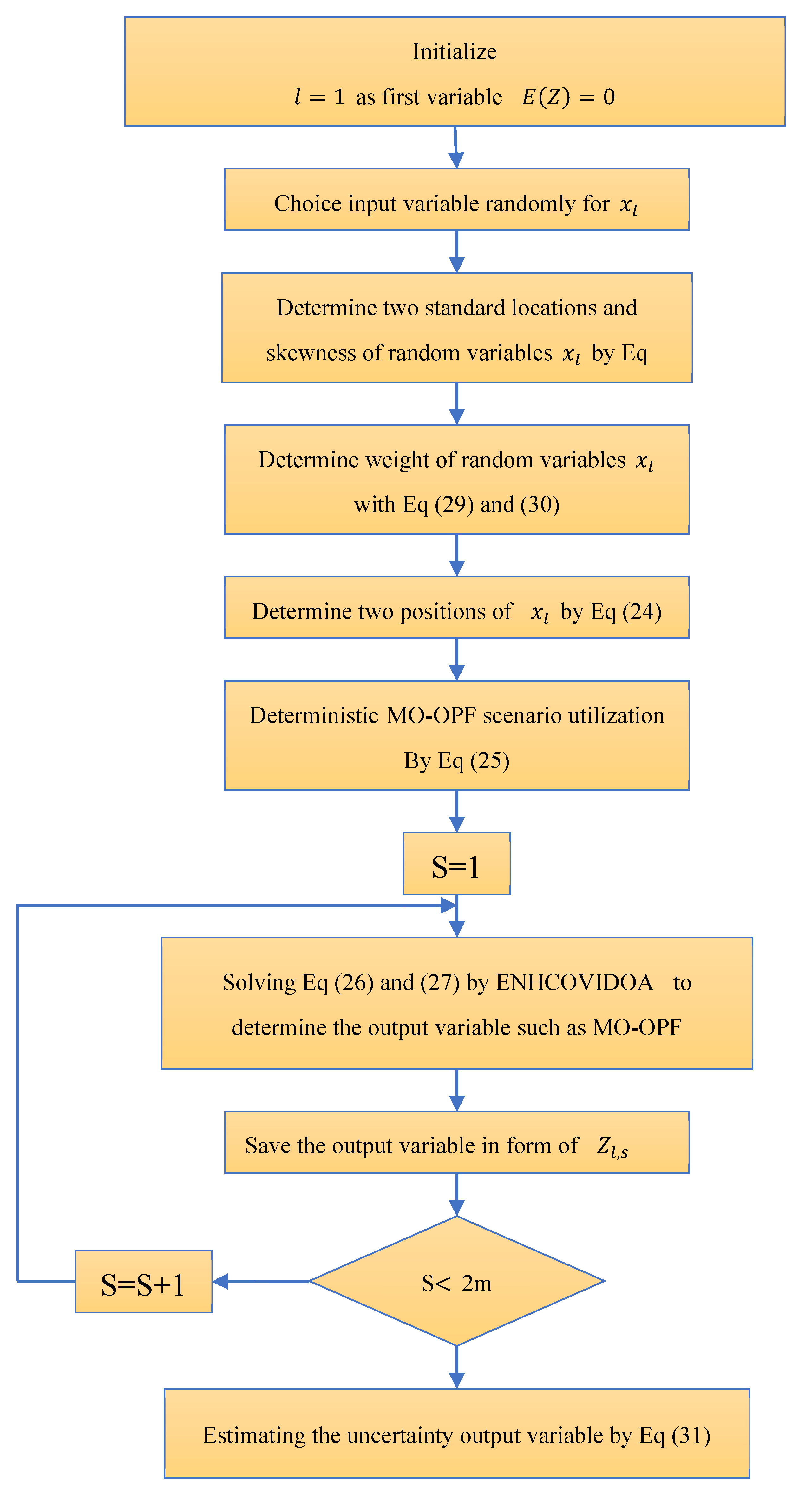
Figure 2.
flowchart of ENHCOVIDOA.
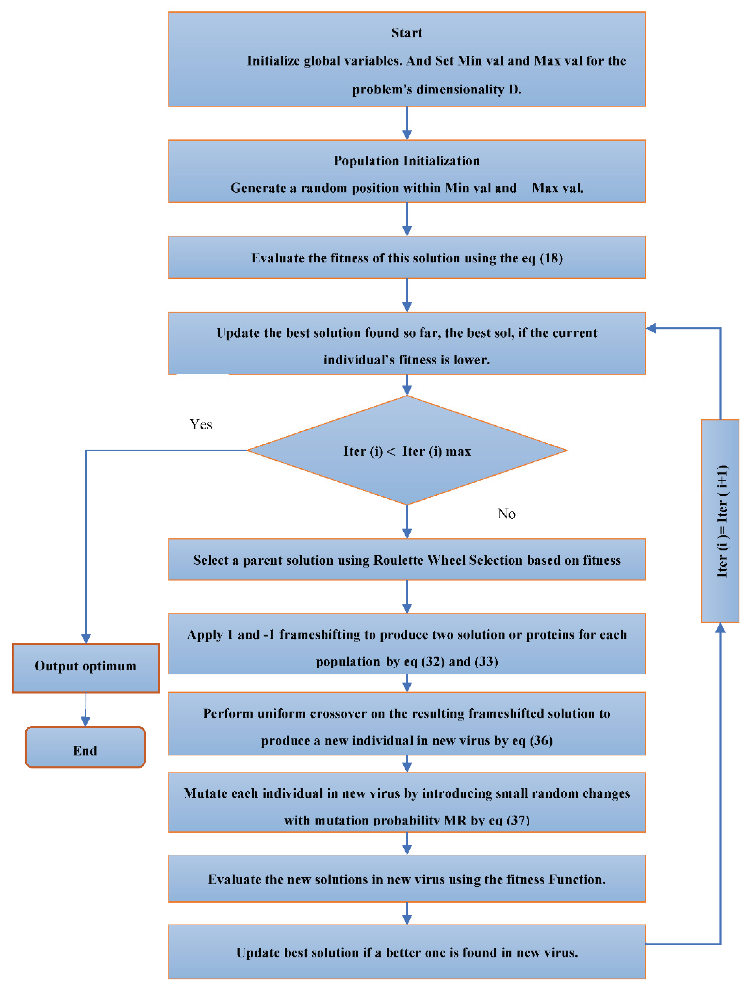
Figure 3.
(a) Convergence characteristic of COVIDO for case 1; (b) Convergence characteristic of ENHCOVIDO for case 2.
Figure 3.
(a) Convergence characteristic of COVIDO for case 1; (b) Convergence characteristic of ENHCOVIDO for case 2.
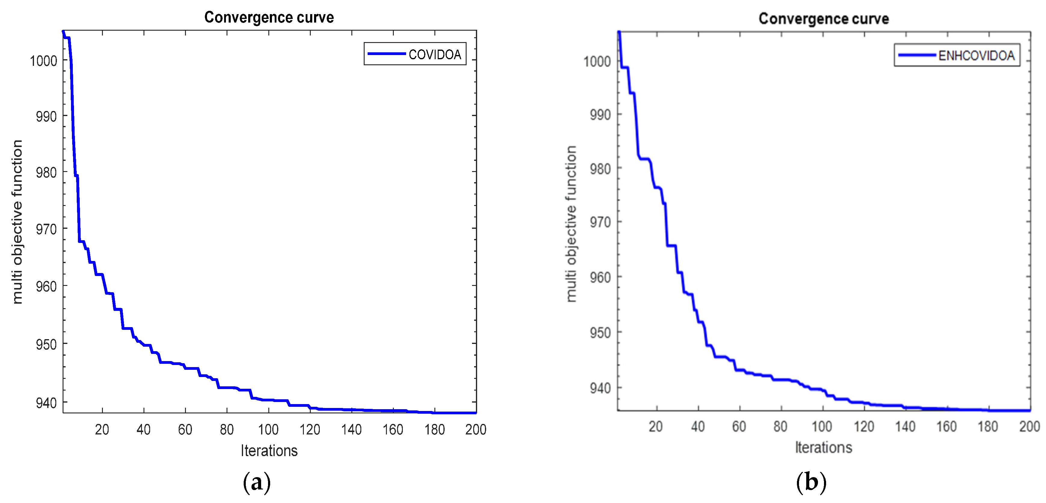
Figure 4.
(a) Voltage deviation provided by COVIDOA for Case 1; (b) Voltage deviation provided by ENHCOVIDOA for Case2.
Figure 4.
(a) Voltage deviation provided by COVIDOA for Case 1; (b) Voltage deviation provided by ENHCOVIDOA for Case2.
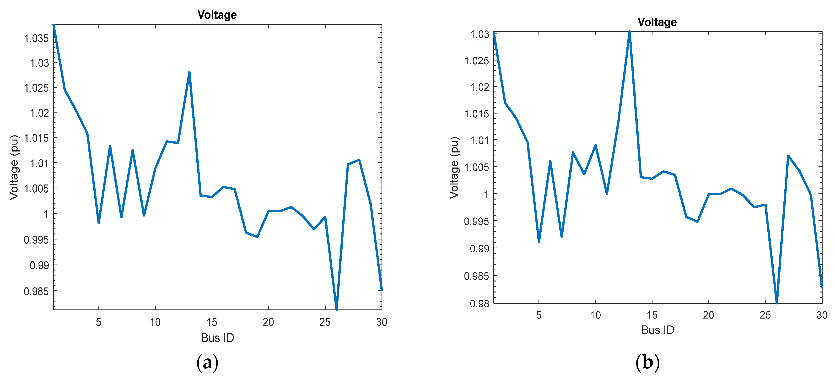
Figure 5.
(a) Convergence characteristic of COVIDOA for case 3; (b) Convergence characteristic of ENHCOVIDO for case 4.
Figure 5.
(a) Convergence characteristic of COVIDOA for case 3; (b) Convergence characteristic of ENHCOVIDO for case 4.
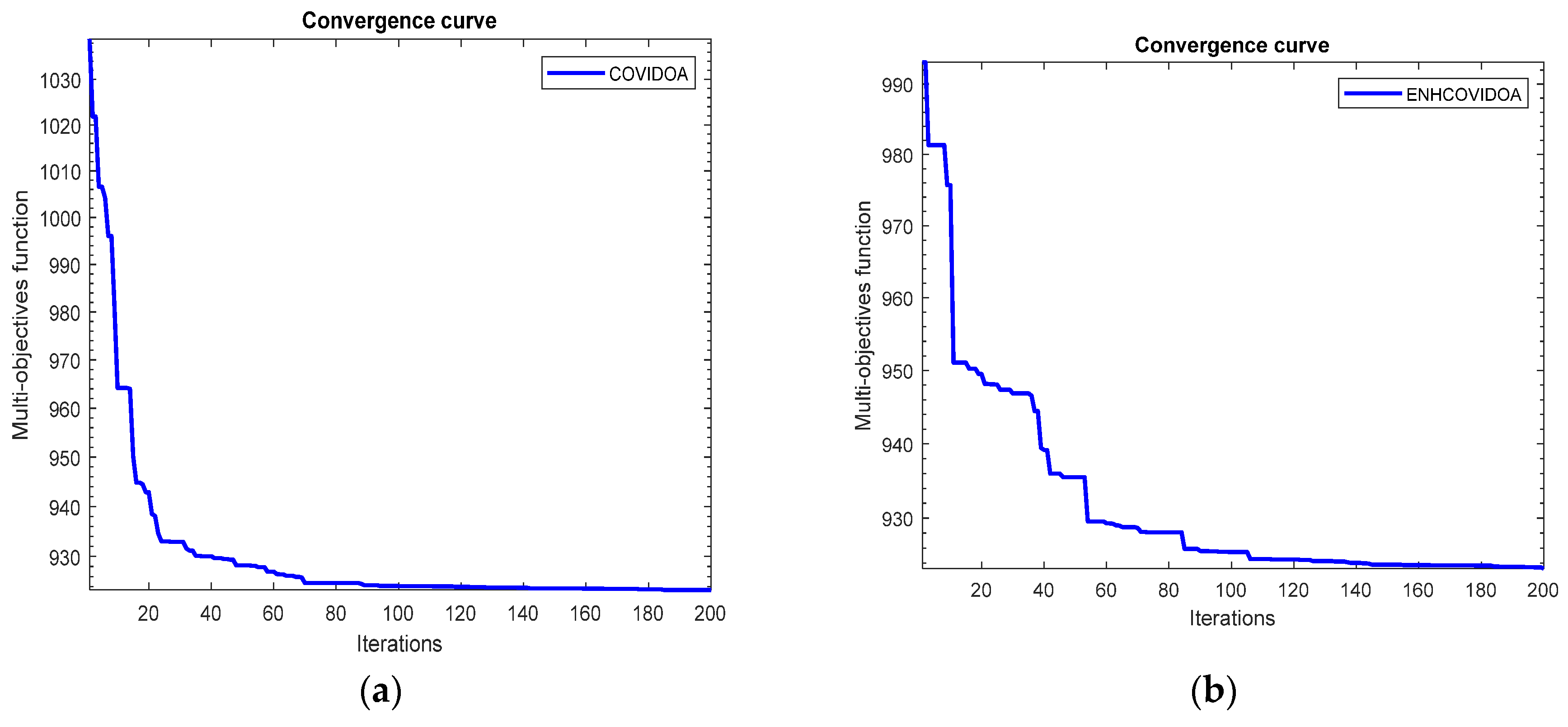
Figure 6.
(a) Voltage deviation provided by COVIDOA of Case 3; (b) Voltage deviation provided by ENHCOVIDOA of Case 4.
Figure 6.
(a) Voltage deviation provided by COVIDOA of Case 3; (b) Voltage deviation provided by ENHCOVIDOA of Case 4.
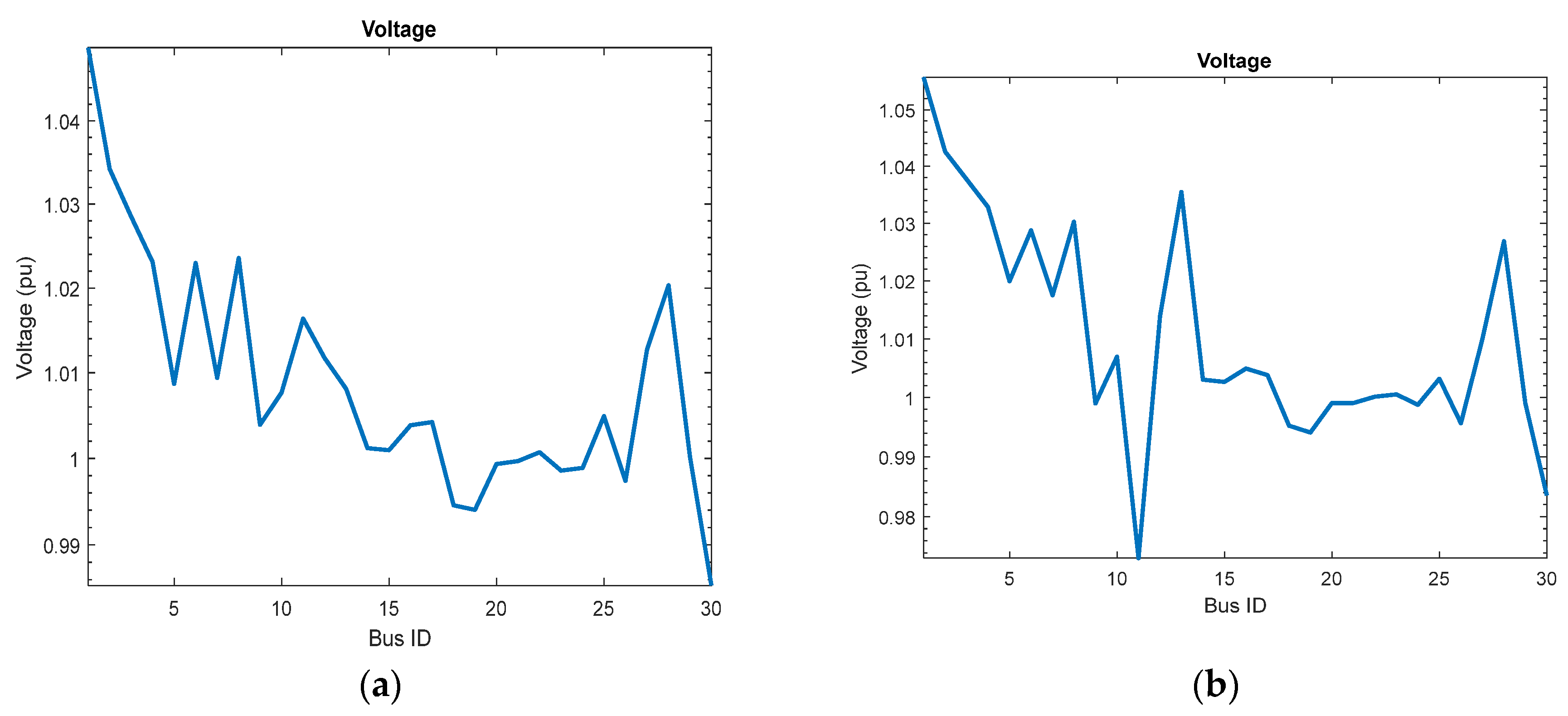
Figure 7.
convergence characteristic of ENHCOVIDOA based on TPEM.
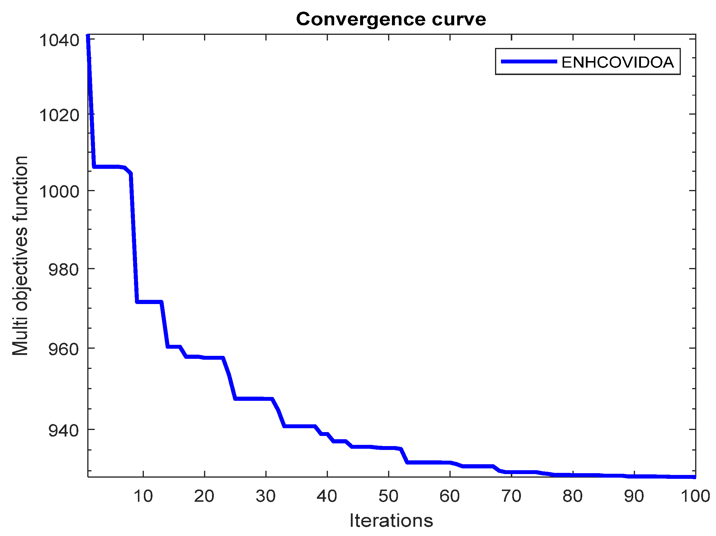
Figure 8.
(a) Convergence characteristic of COVIDOA for case 6; (b) Convergence characteristic of HENCOVIDOA for case 7.
Figure 8.
(a) Convergence characteristic of COVIDOA for case 6; (b) Convergence characteristic of HENCOVIDOA for case 7.
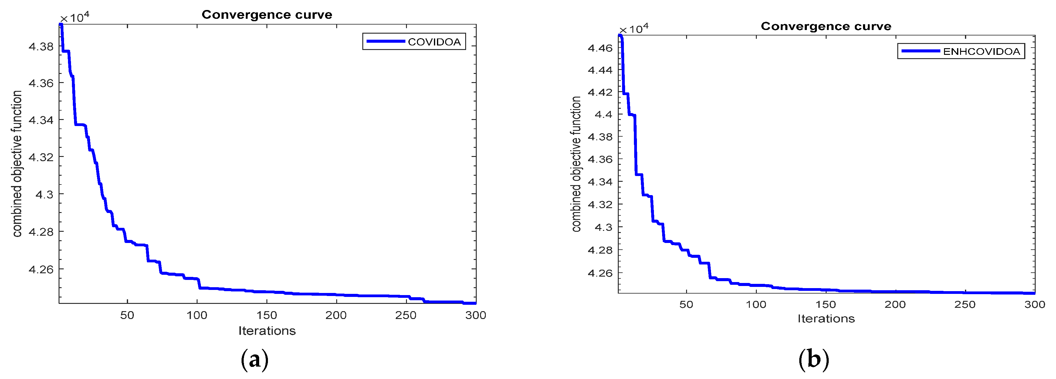
Figure 9.
(a) Voltage deviation provided by COVIDOA for Case 6; (b) Voltage deviation provided by ENHCOVIDOA for Case 7.
Figure 9.
(a) Voltage deviation provided by COVIDOA for Case 6; (b) Voltage deviation provided by ENHCOVIDOA for Case 7.
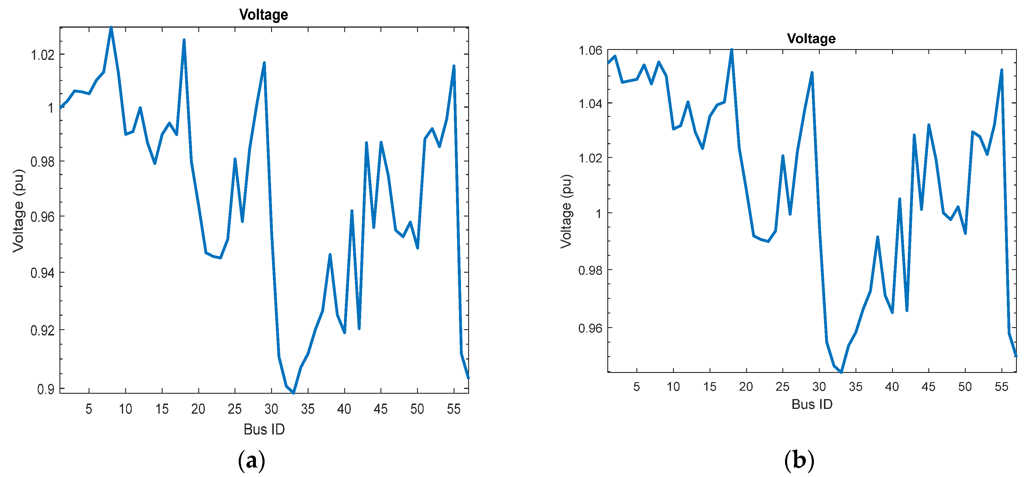
Figure 10.
convergence characteristic of TPEM-ENHCOVIDOA for case 10.
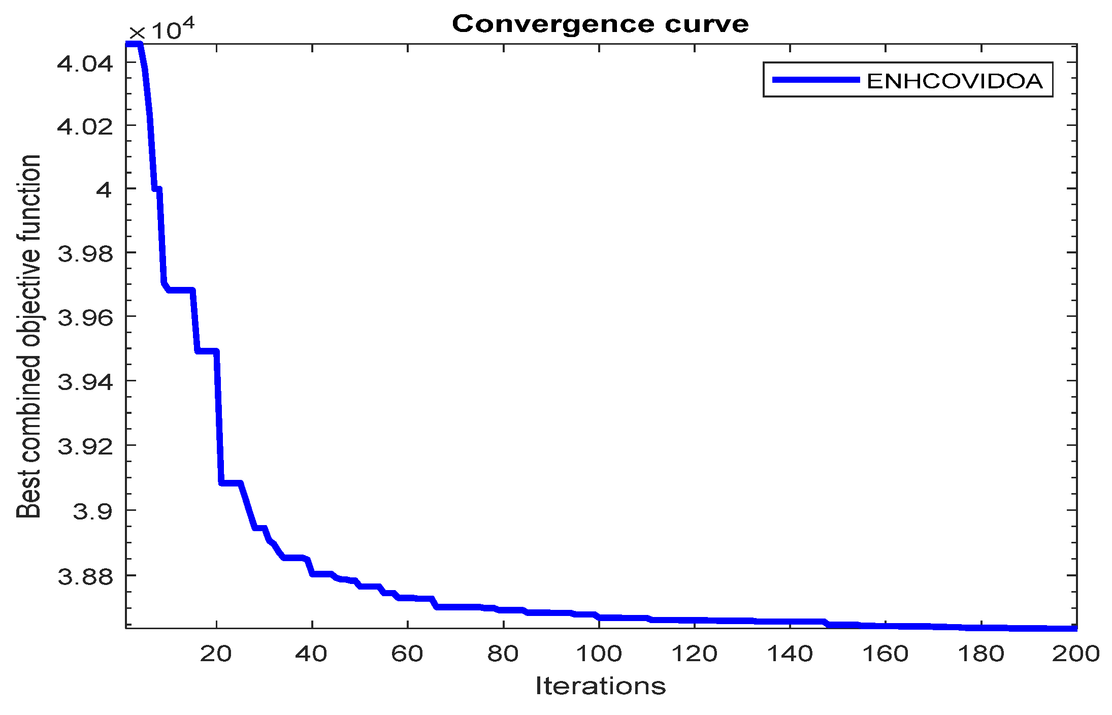
Table 1.
OPF results with optimum values of control variables for IEEE 30-bus system.
| Control variables | min | max | Case 1 | Case 2 | Case3 | Case 4 | Case 5 |
|---|---|---|---|---|---|---|---|
| Pg1(MW) | 50 | 200 | 140.2514 | 134.5761 | 134.6114 | 139.9049 | 130.1052 |
| Pg2(MW) | 20 | 80 | 50.43805 | 53.1141 | 48.70912 | 50.29628 | 50.1031 |
| Pg5(MW) | 15 | 50 | 27.80691 | 27.8523 | 29.05698 | 29.48819 | 27.49195 |
| Pg8(MW) | 10 | 35 | 35.34707 | 35.1804 | 34.07451 | 32.31542 | 33.62404 |
| Pg11(MW) | 10 | 30 | 19.489 | 22.2084 | 23.20275 | 21.42332 | 23.39687 |
| Pg13(MW) | 12 | 40 | 20.96857 | 18.9320 | 18.29716 | 15.3875 | 19.33414 |
| Q10(MVAr) | 0 | 5 | 4.595368 | 1.9572 | 3.578709 | 2.451346 | 3.17631 |
| Q12(MVAr) | 0 | 5 | 2.055626 | 1.0990 | 2.804495 | 0.465449 | 2.40793 |
| Q15(MVAr) | 0 | 5 | 4.402551 | 4.4817 | 4.187433 | 3.135117 | 0.53022 |
| Q17(MVAr) | 0 | 5 | 1.931677 | 3.8037 | 4.575689 | 4.725294 | 2.14841 |
| Q20(MVAr) | 0 | 5 | 4.550504 | 4.9286 | 3.436736 | 4.482416 | 1.60314 |
| Q21(MVAr) | 0 | 5 | 2.947572 | 4.6435 | 4.675022 | 4.528572 | 2.18216 |
| Q23(MVAr) | 0 | 5 | 2.544655 | 2.3785 | 1.870116 | 2.815127 | 1.78985 |
| Q24(MVAr) | 0 | 5 | 4.82601 | 3.5773 | 4.627495 | 4.96885 | 2.93594 |
| Q29(MVAr) | 0 | 5 | 4.300718 | 4.1293 | 2.424171 | 3.06705 | 1.08940 |
| Tr6-9 p.u | 0.9 | 1.1 | 1.006707 | 1.044504 | 1.014857 | 1.016047 | 1.05741 |
| Tr6-10 p.u | 0.9 | 1.1 | 1.021691 | 1.014578 | 1.051505 | 1.056226 | 1.01909 |
| Tr4-12 p.u | 0.9 | 1.1 | 1.009127 | 1.00571 | 1.023904 | 1.029375 | 1.01495 |
| Tr27-28 p.u | 0.9 | 1.1 | 0.990478 | 0.991432 | 1.003469 | 1.00641 | 1.01421 |
| VG1 p.u | 0.94 | 1.06 | 1.030368 | 1.037668 | 1.057574 | 1.0558 | 1.09406 |
| VG2 p.u | 0.94 | 1.06 | 1.016942 | 1.024458 | 1.046787 | 1.042571 | 1.08053 |
| VG3 p.u | 0.94 | 1.06 | 0.99113 | 0.998129 | 1.019273 | 1.019921 | 1.05439 |
| VG4 p.u | 0.94 | 1.06 | 1.007653 | 1.012465 | 1.035755 | 1.030266 | 1.0591 |
| VG5 p.u | 0.94 | 1.06 | 0.99996 | 1.014189 | 0.970747 | 0.973151 | 1.01485 |
| VG6 p.u | 0.94 | 1.06 | 1.030428 | 1.028067 | 1.023615 | 1.03548 | 1.01028 |
| cost ($/h) | ------ | ----- | 830.2781 | 825.9120 | 812.6197 | 810.12 | 799.959 |
| loss (MW) | ------ | ----- | 5.9010 | 6.0336 | 5.2519 | 5.415597 | 5.65531 |
| VD p.u | ------ | ----- | 0.1606 | 0.1411 | 0.2441 | 0.2293 | 0.2322 |
| Emission(ton/h) | ------ | ----- | 0.2449 | 0.2405 | 0.2372 | 0.231231 | 0.2516 |
Table 2.
Results of the proposed methods and other methods for case 1 &2 without DG.
| Papers | Method | Fuel cost $/h | Loss power (MW) | Emissions ton/h | V.D p.u |
|---|---|---|---|---|---|
| [4] | COA | 830.2933 | 5.7225 | 0.2558 | 0.3319 |
| [4] | MCOA | 830.2793 | 5.5876 | 0.2529 | 0.2971 |
| [21] | TFWO | 826.779 | 5.459 | 0.255 | 0.459 |
| [22] | SMA | 832.3665 | 6.4495 | 0.2675 | 0.2189 |
| [23] | J-PPS1 | 830.9938 | 5.612 | 0.2355 | 0.299 |
| [23] | J-PPS2 | 830.8672 | 5.6175 | 0.2357 | 0.2948 |
| [23] | J-PPS3 | 830.3088 | 5.6377 | 0.2363 | 0.949 |
| [23] | Jaya | 831.5493 | 5.578 | 0.23582 | 0.31147 |
| [24] | AGTLBO | 830.1559 | 5.5823 | 0.2529 | 0.2975 |
| [24] | TLBO | 831.3186 | 5.5847 | 0.2538 | 0.2982 |
| [34] | HHO | 906.52 | 4.21 | 0.297 | ----------- |
| [37] | PSO-SSO | 826.94 | 5.515 | 0.258 | 0.466 |
| Present paper | COVIDOA | 830.2781 | 5.9010 | 0.2449 | 0.1606 |
| proposal | ENHCOVIDOA | 825.9120 | 6.0336 | 0.2405 | 0.1411 |
Table 3.
Results of the proposed methods and other methods for case 3 &4 with DG.
| Paper | Method | Fuel cost ($/h) |
Power loss (MW) |
Emission (ton/h) | Voltage deviation p.u | Combined objective function ($/h) |
|---|---|---|---|---|---|---|
| [23] | DA | 811.9476 | 5.2318 | 0.2328 | 0.3385 | 938.5816 |
| [23] | GWO | 811.2105 | 5.2836 | 0.2340 | 0.3142 | 938.4980 |
| [23] | Jaya | 812.3347 | 5.2871 | 0.2327 | 0.2525 | 938.3787 |
| [23] | J-PPS1 | 811.9609 | 5.2381 | 0.2329 | 0.2875 | 937.6646 |
| [23] | J-PPS2 | 811.8993 | 5.2171 | 0.2330 | 0.2990 | 937.3837 |
| [23] | J-PPS3 | 811.8635 | 5.2214 | 0.2329 | 0.2946 | 937.3486 |
| [34] | HHO | 905.19 | 4.02 | 0.219 | ---------- | ------------- |
| Present paper | COVIDOA | 812.6197 | 5.2519 | 0.2372 | 0.2441 | 925.0389 |
| Proposal | HENCOVIDOA | 810.12 | 5.41559 | 0.231231 | 0.2293 | 922.4154 |
Table 4.
Mean, and standard deviations of multi objectives of optimal power flow with ieee-30 buses.
Table 4.
Mean, and standard deviations of multi objectives of optimal power flow with ieee-30 buses.
| objectives | Mean value of objectives in case (4) | Mean value of objectives in case (5) |
Standard deviation value of objectives | Percentage error of objectives % |
|---|---|---|---|---|
| Cost $/h | 810.12 | 799.9597 | 26.1802 | 1.2540 |
| Power loss (MW) | 5.415597 | 5.655313 | 0.2207 | 4.238 |
| Emission ton/h | 0.23123 | 0.23169 | 0.00551 | 0.1989 |
| V.D p.u | 0.2293 | 0.2322 | 0.08106 | 0.22 |
Table 5.
OPF results with optimum values of control variables for IEEE 57-bus system.
| Control variables | Min | Max | Case 6 | Case 7 | Case 8 | Case 9 | Case 10 |
|---|---|---|---|---|---|---|---|
| PG1(MW) | 0.0 | 576 | 147.7466 | 147.3466 | 138.2847 | 139.4484 | 126.3896 |
| PG2(MW) | 30 | 100 | 76.90452 | 76.90452 | 55.91601 | 64.024 | 82.52883 |
| PG3(MW) | 40 | 140 | 44.96443 | 44.96443 | 47.05652 | 44.3149 | 43.49 |
| PG6(MW) | 30 | 100 | 82.88241 | 82.28241 | 66.60258 | 56.42907 | 77.60407 |
| PG8(MW) | 100 | 550 | 440.0902 | 440.0902 | 396.2878 | 414.49 | 416.4948 |
| PG9(MW) | 30 | 100 | 91.28159 | 91.18159 | 85.92483 | 76.05979 | 62.79682 |
| PG12(MW) | 100 | 410 | 382.655 | 382.155 | 378.8193 | 374.7441 | 359.8531 |
| VG1 p.u | 0.94 | 1.06 | 1.05486 | 1.05486 | 0.999617 | 0.999848 | 1.014681 |
| VG2 p.u | 0.94 | 1.06 | 1.057506 | 1.057506 | 1.002474 | 1.003335 | 1.024809 |
| VG3 p.u | 0.94 | 1.06 | 1.047676 | 1.047676 | 0.997826 | 1.001074 | 1.021833 |
| VG6 p.u | 0.94 | 1.06 | 1.054179 | 1.054179 | 1.006701 | 1.013864 | 1.027252 |
| VG8 p.u | 0.94 | 1.06 | 1.055289 | 1.055289 | 1.029734 | 1.03665 | 1.055995 |
| VG9 p.u | 0.94 | 1.06 | 1.050137 | 1.050137 | 1.017335 | 1.019945 | 1.047834 |
| VG12 p.u | 0.94 | 1.06 | 1.040447 | 1.040447 | 0.999728 | 1.001865 | 1.027677 |
| T4-18 p.u | 0.9 | 1.1 | 1.083404 | 1.083404 | 1.002931 | 0.992828 | 0.967174 |
| T4-18 p.u | 0.9 | 1.1 | 1.078778 | 1.078778 | 1.038215 | 1.080058 | 0.952725 |
| T21-20 p.u | 0.9 | 1.1 | 0.992588 | 0.992588 | 1.03737 | 1.061319 | 0.947047 |
| T24-25 p.u | 0.9 | 1.1 | 1.024639 | 1.024639 | 1.028365 | 1.081288 | 0.918847 |
| T24-25 p.u | 0.9 | 1.1 | 0.996758 | 0.996758 | 1.042208 | 1.089272 | 0.99157 |
| T24-26 p.u | 0.9 | 1.1 | 1.033145 | 1.033145 | 1.092891 | 1.095885 | 0.985932 |
| T7-29 p.u | 0.9 | 1.1 | 0.992827 | 0.992827 | 0.990088 | 0.992962 | 1.019252 |
| T34-32 p.u | 0.9 | 1.1 | 1.083837 | 1.083837 | 1.001526 | 1.031651 | 0.919699 |
| T11-41 p.u | 0.9 | 1.1 | 1.067665 | 1.067665 | 1.023986 | 1.022516 | 0.994203 |
| T15-45 p.u | 0.9 | 1.1 | 1.004601 | 1.004601 | 1.092798 | 0.99325 | 0.994758 |
| T14-46 p.u | 0.9 | 1.1 | 1.020462 | 1.020462 | 1.026692 | 1.007397 | 0.953022 |
| T10-51 p.u | 0.9 | 1.1 | 0.995079 | 0.995079 | 1.027912 | 1.038841 | 0.987867 |
| T13-49 p.u | 0.9 | 1.1 | 1.018602 | 1.018602 | 1.07377 | 1.072386 | 0.904351 |
| T11-43 p.u | 0.9 | 1.1 | 1.08058 | 1.08058 | 1.038348 | 1.095747 | 0.941726 |
| T40-56 p.u | 0.9 | 1.1 | 1.02203 | 1.02203 | 1.066259 | 1.085865 | 0.969629 |
| T39-57 p.u | 0.9 | 1.1 | 1.085325 | 1.085325 | 1.045029 | 1.019932 | 1.016022 |
| T9-55 p.u | 0.9 | 1.1 | 1.094524 | 1.094524 | 1.003751 | 1.006241 | 0.965147 |
| Qc18 (MVAr) | 0.0 | 20 | 7.853548 | 7.853548 | 10.80543 | 9.883294 | 15.63243 |
| Qc25 (MVAr) | 0.0 | 20 | 7.137135 | 7.137135 | 16.33461 | 13.77547 | 5.431922 |
| Qc53 (MVAr) | 0.0 | 20 | 16.18947 | 16.18947 | 15.58332 | 8.537731 | 10.88658 |
| Fuel cost ($/h) | --------- | --------- | 41789.3378 | 41720.67 | 37852.000 | 37799.000 | 37753.7149 |
| power loss(MW) | --------- | --------- | 14.1550 | 14.1249 | 13.2619 | 13.8806 | 13.5276 |
| Emission(ton/h) | --------- | --------- | 1.32605 | 1.3252 | 1.1997 | 1.1965 | 1.1551 |
| V.D p.u | -------- | -------- | 1.4101 | 1.396422 | 0.7894 | 0.7754 | 0.83219 |
Table 6.
Results of the proposed methods and other methods for case 6 &7 without DG.
| Papers | Method | Fuel cost $/h |
Power loss (MW) | Emission (ton/h) | VD p.u |
|---|---|---|---|---|---|
| [23] | DA | 42,584.46 | 13.6065 | 1.3577 | 0.8124 |
| [23] | GWO | 42,587.97 | 13.2727 | 1.3447 | 0.7921 |
| [23] | Jaya | 42,547.09 | 12.772 | 1.3708 | 0.8202 |
| [23] | J-PPS1 | 42,575.97 | 12.5408 | 1.3336 | 0.7893 |
| [23] | J-PPS2 | 42,580.09 | 12.5242 | 1.3433 | 0.7251 |
| [23] | J-PPS3 | 42,564.46 | 12.5079 | 1.3566 | 0.7365 |
| [24] | TLBO | 41,932.01 | 11.5285 | 1.4357 | 0.9528 |
| [24] | AGTLBO | 41,929.39 | 13.2563 | 1.4328 | 0.9526 |
| [36] | MODA | 43897 | 16.7039 | 1.6312 | 0.004 |
| [38] | MOICA | 41,998.57 | 13.3353 | 1.7605 | 0.8748 |
| [38] | MOMICA | 41983.06 | 13.6969 | 1.496 | 0.797 |
| Present paper | COVIDOA | 41789.3378 | 14.1550 | 1.32605 | 1.4101 |
| proposal | ENHCOVIDOA | 41720.67 | 14.1249 | 1.3252 | 1.396422 |
Table 7.
Results of the proposed methods and other methods for case 8 &9 with DG.
| Papers | Method | Fuel cost ($/h) | Power loss (MW) | Emission (ton/h) | Voltage deviation p.u | Combined objective function ($/h) |
|---|---|---|---|---|---|---|
| [23] | DA | 38,120.833 | 12.3189 | 1.2751 | 0.5454 | 39,200.17 |
| [23] | GWO | 38,114.735 | 13.1703 | 1.3099 | 0.4504 | 39,173.097 |
| [23] | Jaya | 38,105.956 | 12.5706 | 1.3218 | 0.4721 | 39,162.889 |
| [23] | J-PPS1 | 38,059.913 | 12.8818 | 1.3035 | 0.5469 | 39,167.596 |
| [23] | J-PPS2 | 38,048.250 | 13.3724 | 1.3612 | 0.5136 | 39,165.964 |
| [23] | J-PPS3 | 38,033.832 | 12.9742 | 1.3115 | 0.5329 | 39,136.324 |
| Present paper | COVIDOA | 37852.000 | 13.2619 | 1.1997 | 0.7894 | 38748.123 |
| proposal | ENHCOVIDOA | 37,799.000 | 13.8806 | 1.1965 | 0.7754 | 38,733.676 |
Table 8.
Mean and standard deviation of multi objectives of optimal power flow with ieee-57 buses.
| objectives | Mean value of objectives in case (9) |
Mean value of objectives in case (10) |
Standard deviation value of objectives |
Percentage error of mean (9) & mean (10) % |
|
|---|---|---|---|---|---|
| Cost $/h | 37799.000 | 37753.7149 | 1175.8062 | 0.1198 | |
| Power loss (MW) | 13.8806 | 13.5276 | 1.2534 | 2.54311 | |
| Emission ton/h | 1.1965 | 1.1551 | 0.0668 | 3.4600 | |
| V.D p.u | 0.7754 | 0.83219 | 0.06986 | 7.3239 |
Table 9.
OPF results with optimum values of control variables for SISGHV-28 buses system. .
| Control variables | Min | Max | Case 11 | Case 12 | Case 13 |
|---|---|---|---|---|---|
| Pg1(MW) | 150 | 1200 | 699.9615 | 618.2087 | 719.1426 |
| Pg2(MW) | 130 | 988 | 492.2544 | 485.9416 | 489.1143 |
| Pg3(MW) | 150 | 750 | 214.1131 | 220.9904 | 215.9316 |
| Pg4(MW) | 120 | 1320 | 187.6118 | 157.4339 | 143.732 |
| Pg5(MW) | 70 | 636 | 86.83202 | 99.40292 | 103.8542 |
| Pg6(MW) | 50 | 260 | 218.9916 | 216.6991 | 225.7888 |
| Pg7(MW) | 180 | 910 | 900.778 | 905.4464 | 871.8454 |
| Pg8(MW) | 60 | 660 | 423.9247 | 402.1977 | 407.9387 |
| Pg9(MW) | 50 | 500 | 364.8132 | 82.70119 | 75.19729 |
| Pg10(MW) | 250 | 1320 | 354.707 | 295.1099 | 296.9072 |
| Pg11(MW) | 250 | 1250 | 403.361 | 731.3575 | 708.5445 |
| Pg12(MW) | 210 | 800 | 622.2266 | 577.7357 | 543.7552 |
| Pg13(MW) | 100 | 940 | 857.7883 | 742.7903 | 731.771 |
| Pg14(MW) | 50 | 250 | 185.3944 | 176.0874 | 170.8831 |
| VG1 p.u | 0.94 | 1.06 | 1.031671 | 0.971935 | 0.980602 |
| VG2 p.u | 0.94 | 1.06 | 1.059468 | 1.058471 | 1.058493 |
| VG3 p.u | 0.94 | 1.06 | 0.943989 | 0.942145 | 0.941001 |
| VG4 p.u | 0.94 | 1.06 | 0.996006 | 1.037361 | 0.946481 |
| VG5 p.u | 0.94 | 1.06 | 0.999072 | 1.040843 | 0.947657 |
| VG6 p.u | 0.94 | 1.06 | 1.021664 | 1.055141 | 0.941425 |
| VG7 p.u | 0.94 | 1.06 | 1.056341 | 1.059461 | 1.000028 |
| VG8 p.u | 0.94 | 1.06 | 1.054181 | 1.05847 | 1.058423 |
| VG9 p.u | 0.94 | 1.06 | 0.941005 | 1.059939 | 1.034749 |
| VG10p.u | 0.94 | 1.06 | 1.056691 | 1.052316 | 1.03147 |
| VG11 p.u | 0.94 | 1.06 | 1.054986 | 1.053859 | 1.032116 |
| VG12 p.u | 0.94 | 1.06 | 1.059054 | 1.055919 | 1.052243 |
| VG13p.u | 0.94 | 1.06 | 1.049867 | 1.047947 | 1.043022 |
| VG14p.u | 0.94 | 1.06 | 0.966548 | 0.961948 | 0.958046 |
| Fuel cost ($/h) | ------ | ----- | 27166.96 | 24053.64 | 23762.34 |
| power loss (MW) | ------ | ------ | 31.37879 | 34.1026 | 32.10262 |
| Emission(ton/h) | ------ | ------ | 0.8038 | 0.7379 | 0.7332 |
| V.D p.u | ------ | ------ | 0.3305 | 0.658 | 0.5408 |
Table 10.
Mean and standard deviation of multi objectives of optimal power flow with SISGHV-28 buses system.
Table 10.
Mean and standard deviation of multi objectives of optimal power flow with SISGHV-28 buses system.
| Objectives | Mean value of objectives in case (12) | Mean value of objectives in case (13) | Standard deviation value of objectives | Percentage error of objectives case12 & case 13 % | |
|---|---|---|---|---|---|
| Cost $/h | 24053.64 | 23762.34 | 896.0824 | 1.2 | |
| Power loss (MW) | 34.1026 | 32.10262 | 7.6639 | 5.8645 | |
| Emission ton/h | 0.7379 | 0.7332 | 0.91397 | 0.6369 | |
| V.D p.u | 0.658 | 0.5408 | 0.01563 | 17.8115 |
Disclaimer/Publisher’s Note: The statements, opinions and data contained in all publications are solely those of the individual author(s) and contributor(s) and not of MDPI and/or the editor(s). MDPI and/or the editor(s) disclaim responsibility for any injury to people or property resulting from any ideas, methods, instructions or products referred to in the content. |
© 2024 by the authors. Licensee MDPI, Basel, Switzerland. This article is an open access article distributed under the terms and conditions of the Creative Commons Attribution (CC BY) license (http://creativecommons.org/licenses/by/4.0/).
Copyright: This open access article is published under a Creative Commons CC BY 4.0 license, which permit the free download, distribution, and reuse, provided that the author and preprint are cited in any reuse.


