Preprint
Article

A New General Correlation for the Influence Parameter in Density Gradient Theory and Peng-Robinson Equation of State for N-Alkanes

This version is not peer-reviewed.

Submitted:

28 October 2024

Posted:

29 October 2024

You are already at the latest version

A peer-reviewed article of this preprint also exists.

Abstract
A new analytical expression is proposed for the reduced influence parameter in Density Gradient Theory when combined with the Peng-Robinson equation of state for 32 n-alkanes. It contains the critical and triple point temperature values for each fluid as input and three adjustable coefficients. The new analytical expression contains the two-coefficients Zuo and Stenby and Miqueu et al.correlations as particular cases, and it is a modification of the previously published Cachadiña et al. correlation. Initially, the correlation coefficients for each fluid were obtained by fitting selected values for surface tension, and the results were comparable to other specific correlations reported in the literature. The overall mean absolute percentage deviation (OMAPD) between the selected and calculated data is just 0.79% Then, a general correlation including six adjustable coefficients valid for all the considered n-alkanes is proposed. It includes the radius of gyration as a new input parameter for each fluid. In this case, the OMAPD is 1.78\%. The use of other fluid properties as inputs is also briefly discussed.
Keywords: 
Subject: 
Physical Sciences  -   Thermodynamics

1. Introduction

The surface tension is regarded as an essential property of liquids in both theoretical and practical studies of different processes such, for instance, bubble and droplet formation, wetting, capillarity, detergency, atomization, formation of aerosols and sprays, injection of fuels, and so others [1,2,3,4,5,6,7]. In particular, pure liquid n-alkanes and their mixtures are commonly used in some industrial processes [8,9,10,11,12,13,14,15,16,17] as, for example, the injection and atomization of fuels in engines or the use of liquefied natural gas as a fuel [8,10,16,18,19,20,21,22,23,24].
In the petroleum industry, the surface tension of n-alkanes has to be considered in the enhanced oil recovery technique, where gases, as CO 2 , of surfactants, are added to reduce the interfacial properties between crude oil and the geological reservoir [25].
Moreover, the knowledge of vapor-liquid equilibrium properties and surface tension of n-alkanes and alcohols is required to study additives commonly used in fuels [12,13,14,26,27], in removing hydrocarbons from liquid effluents [28,29], and in the study of carbon dioxide capture and storage technologies [17,30,31,32]. In this last case, high pressures and temperatures are needed, which are not always easily accessible.
In the study of the aforementioned applications, it is necessary to have surface tension values for both pure fluids and mixtures, especially for the longest or heaviest n-alkanes, in a wide range of temperatures, or to have reliable and accurate models or methods to calculate or predict them with reasonable extrapolation and prediction capabilities [17,31].
Some semi-theoretical methods, such as computer simulations, the application of the density gradient theory (DGT) together with an equation of state (EoS), and others have already been applied to the surface tension of pure n-alkanes and some mixtures containing them [13,14,29,31,33,34,35,36,37,38,39,40,41,42,43,44,45,46,47]. The main advantages of these methods are that they are based on some theoretical approaches and that, apart from the surface tension, other interface properties can be calculated. However, as expected, these general models are sometimes not accurate enough.
For instance, the computer simulation results available presently only lead to reproducing qualitatively the experimental values [15,31,35,41,43,45]. In the case of DGT+EoS method results exhibit good performance, but usually limited within to specific temperature regions, often at low temperatures [13,14,29,31,33,34,37,38,39,40,42,44,46]. On the other hand, the use of computer simulations and DGT+EoS method requires the use of specific software or the development of complex computer programs [47], so they cannot be considered straightforward ones. A comprehensive summary of these models was performed in Ref. [17].
In particular, the DGT+EoS model is one of the most used [13,14,29,33,34,37,41,42,43,44,47]. Basically, this method considers the use of the EoS to obtain the vapor-liquid equilibrium densities and then the DGT to relate them with the available values of the surface tension, which permits to calculate the so-called “influence parameter”. As the value of this parameter depends on the fluid and temperature considered, it is useful to have correlations allowing its calculation from the values of some fixed properties of the fluid, i.e., its triple point temperature, acentric factor, molar volume, critical temperature, etc. [33,42,48,49].
Two examples of the use of the DGT+EoS model to obtain the surface properties of pure alkanes can be mentioned here. One is the molecular parametrization based on a new version of the statistical associating fluid theory (SAFT) EoS proposed by Mejía et al. [43]. A qualitative comparison of the results obtained for the surface tension of n-hexane and 5-nonanone showed a good agreement when compared with some experimental results. Following a similar procedure but using a different version of the SAFT EoS, Garrido et al. [44] obtained results for the surface tension of 15 pure fluids, including some n-alkanes. The deviations from the experimental data were below 4.8%, with the overall absolute average deviation being 2.4%. As is said, a summary of the results obtained with this kind of model for different types of fluids is available in Ref. [17].
On the other hand, purely empirical or semiempirical methods such as artificial neural networks, group-contribution methods, quantitative structure-property relationships, corresponding states’ principle methods, or combinations of them have also been applied to obtain the surface tension of n-alkanes [46,50,51,52,53,54,55,56,57,58,59,60,61,62,63,64,65,66,67,68,69,70,71,72]. Nevertheless, the obtained results are not entirely satisfactory because of the limited number of fluids and/or data considered. Thus, in many cases, the number of data sources considered was very scarce (or even just one). Moreover, a previous selection or comparison between the data available from different sources was not made in most cases.
In a previous paper, we found significant differences between the values provided for different sources for the surface tension of n-alkanes [73]. This fact encourages us to select the more appropriate ones, and this data selection has been updated here to serve as a reference for the application of the DGT+EoS method for n-alkanes, as described below.
The DGT+EoS method requires calculating the influence parameter from surface tension data at different temperatures. Apart from having a collection of data for the influence parameter of different fluids and temperatures, it would be desirable to have a general correlation, including general coefficients valid for at least one family of fluids, that gave accurate results and that had the predictive capacity to apply it to other fluids of the same or similar family and also to mixtures of them.
In a previous paper (Cachadiña et al. [49]), a correlation for the influence parameter of a group of esters was developed and applied. The proposed analytical expression includes two adjustable coefficients for each ester and a common exponent for all esters. This exponent holds a physical significance as it is linked to the universal scaling law. The new correlation effectively replicates the surface tension of 39 esters, yielding an overall deviation of 1.37%.
Following a similar procedure, the main aim of this paper is to propose a general correlation for the influence parameter of n-alkanes. The Peng-Robinson equation of state [74,75] is used to obtain the vapor-liquid equilibrium densities for each temperature. Then the DGT is applied to obtain the influence parameter values in a wide range of temperatures by taking the values for the surface tension selected from different data sources (databases, books and papers) as referents.
Then, different correlations are considered to fit these data into an analytical expression that could reproduce them accurately for each fluid. Then, a generalized expression is used, which permits obtaining the influence parameter and then the surface tension of n-alkanes by using adjustable coefficients and some fixed thermodynamic properties for each fluid as input parameters.
This paper is organized as follows. First, the general expressions for the DGT and the Peng-Robinson EoS are introduced. Moreover, some advantages and disadvantages of using this method are summarized. Section 3 describes the surface tension dataset that has been considered. In Section 4, some previous correlations to obtain the influence parameter as a function of the temperature are analyzed. Then, a new correlation is proposed for the case of n-alkanes. Results are shown in Section 5, and, finally, conclusions are summarized in Section 6.

2. Density Gradient Theory And Peng-Robinson Equation Of State.

The Density Gradient Theory, developed by Cahn and Hilliard [76], and later used in combination with an equation of state by Carey et al. [77], has been successfully applied for years to correlate and predict the surface tension of pure fluids and their mixtures [33,48,77,78,79,80,81,82].
The DGT+EoS method leads to the calculation of the surface tension σ at a given temperature T through the following expression [44,77]:
σ = ρ V 0 ρ L 0 2 c f 0 ρ f 0 ρ T 0 + p 0 d ρ ,
where ρ is the density, ρ V 0 and ρ L 0 are the saturated vapor and liquid densities at temperature T, p 0 is the saturation pressure, and c is the influence parameter, which can be considered to be only temperature-dependent.
The Helmholtz energy density f 0 is defined as:
f 0 ( ρ , T ) = ρ f ( ρ , T ) ,
where f ( ρ , T ) is the Helmholtz energy of the system. As explained in Ref. [49], the Helmholtz energy is the sum of the ideal part ( f ) and the residual part ( f r ) , that is f = f + f r . The ideal part f is obtained from the ideal isobaric caloric capacity c p ( T ) , while the residual can be determined from the analytical expression of pressure (p) as:
f r ( ρ , T ) = p ρ 2 d ρ R T log ρ .
As it is demonstrated in Ref. [49], the result for the integration included in (1) is independent of the ideal contribution ( f ). Thus, the ideal contribution f 0 in (1) can be replaced by f 0 r = ρ f r ( ρ , T ) , and then the values for c p ( T ) are indeed not necessary.
It is important to note that the DGT+EoS method presents some advantages when compared with others:
i) It is theoretically sound, as the fundamentals of the van der Waals theory are applied. The system inhomogeneities are given as a function of the gradient density and can be expressed as a function of the direct correlation function [76,83].
ii) The coexistence densities at the vapor-liquid equilibrium and the saturation pressure are obtained directly from the EoS, so other data sources or analytical expressions are not needed.
iii) It permits the calculation of the surface or interfacial tension values as well as the density profiles and their thickness, the surface enthalpy and entropy, and some relevant properties for the adsorption processes [79].
On the other hand, the DGT+EoS method has certain limitations. According to Liang et al. [84], the method is not entirely general and does not always permit making predictions. A fitting procedure is needed to obtain the influence parameter, and its values, or the correlations proposed to calculate it, are not always transferable to other substances or temperature ranges [44,85]. Finally, the required calculations are not always straightforward and must be made carefully to avoid wrong results.
Besides, when applying the DGT+EoS, it has to be noted that [49]:
i) The influence parameter values will depend on the EoS used; ii) Usually the EoS were designed without paying much attention to the behavior in the region between the liquid and vapor densities, being this region taken into consideration only in the Maxwell-construction that leads to the equal-area equilibrium condition; and iii) The argument of the square root in Equation (1) must be positive: an accurate EoS with multiple van der Waals loops could lead to a negative argument, and the method could be not applicable.
Despite these limitations, the mentioned advantages are valuable, and the DGT+EoS method has been widely used with accurate results for both pure fluids and mixtures, considering different analytical expressions for the EoS and the influence parameter [33,37,42,44,48,77,78,84,85,86,87,88,89,90,91,92,93,94].
A critical decision in using the DGT+EoS method is the choice of an adequate equation of state. In 1978, Carey et al. [77] applied for the first time this method and they used a cubic equation of state, in particular the Peng-Robinson (PR) one. According to Garrido et al. [44], more than 150 scientific papers related to the gradient theory had been published up to 2016, and today the number has been greatly increased. In addition, they highlighted that the most used equations are PR EoS and Statistical-Associating-Fluid-Theory (SAFT) variations. On the other hand, Chow et al. [86], and Larsen et al. [88], reported that Soave-Redlich-Kwong and Cubic-Plus-Association were other widely used equations of state.
The EoS chosen in this work to model the bulk properties of the considered n-alkanes is the Peng-Robinson one [75], known as PR78, as it yields more accurate vapor pressure predictions for heavy hydrocarbons [46,95,96,97].
The PR78 EoS is written as:
p = R T v b a ( v + b ) 2 2 b 2 ,
where v = ρ 1 is the molar volume, R the ideal gas constant, a is the cohesive parameter and b the covolume parameter. The values of a and b are calculated from the critical temperature T c , critical pressure p c , and acentric factor ω , as [75,97]:
a = 0.45724 ( R T c ) 2 p c α ( T )
b = 0.07780 R T c p c
α ( T ) = 1 + m 1 T T c 2
m = 0.37464 + 1.5422 ω 0.26992 ω 2 if ω 0.491 0.379642 + 1.48503 ω 0.164423 ω 2 + 0.016666 ω 3 if ω > 0.491
being α ( T ) known as the thermal cohesion function.
The main improvement in PR78 EoS with respect to the original one [74], is the use of different correlations for m according to smaller o larger values of the acentric factor. As it is known, for the heaviest n-alkanes, the acentric factors are larger. So Equation (8) permits to obtain better results for the properties of the n-alkanes with a higher number of carbons when compared with other previous EoSs [75,95,97].
Once the EoS has been selected, the next step in applying the DGT+EoS method is to consider a set of data for the surface tension of the fluids considered. The procedure followed and the final data selection are explained in the next Section.

3. Sources Of Data

Despite surface tension values can be found in some papers, books, and databases, those data need to be screened and adequately selected, as sometimes there are apparent disagreements between data from different sources [73,98,99,100,101,102,103].
Recently, Mulero et al. [73] performed an extensive search to collect the surface tension data available for 33 n-alkanes, using DIPPR [104] and DETHERM [105] databases, and Wohlfarth and Wohlfarth’s books [106,107,108] as primary sources, and adding some very recently published data. After a screening process, they finally built a database containing 2561 values. They proposed specific correlations (containing two, four, or six adjustable coefficients for each fluid) that permit obtaining the surface tension as a function of the temperature of the fluid and its critical temperature. These correlations reproduce the selected data with mean absolute percentage deviations for each fluid below 2.1% and percentage deviations below 10% except for 9 data (which are close to the critical point, where percentage deviations are high no matter the model or correlation used) [73]. Also, from this work, it is clear that the primary source of the deviations is the data dispersion rather than a bad functional form, so it is not expected to find a specific or general correlation yielding lower mean absolute deviations than the ones reported by Mulero et al. [73].
This work considers an upgraded version of the DIPPR [109] database. The main changes from the version used by Mulero et al. [73] are minor corrections of the critical, triple, and normal boiling point temperatures and the addition of some predicted surface tension data obtained by using Sugden’s correlation [110]. Thus, finally, 2681 values of surface tension data have been considered in this work.
In Figure 1, the reduced temperature location of the available data as a function of the carbon number is shown. It can be seen that, only for the lower n-alkanes, there are surface tension values above the normal boiling point different from Sugden’s DIPPR data. Then, the results obtained for these heavier n-alkanes must be taken cautiously.

4. New Correlation For The Reduced Influence Parameter

To obtain a correlation for the influence parameter in n-alkanes, the following step is to calculate it at each temperature, taking as a referent the selected values for the surface tension. Thus, from Equation (1), the value of influence parameter, c ( T i ) , can be obtained at each temperature at which a surface tension datum ( σ i ) is available, as [49]:
c ( T i ) = σ i 2 ρ V 0 ρ L 0 2 f 0 ρ f 0 ρ T 0 + p 0 d ρ 2 .
To take into account the parameters of the selected EoS and to facilitate the calculations, a reduced influence parameter ( c * ) is defined as [33,48,78,111]:
c * = c a b 2 / 3 ,
being a and b the parameters of the EoS (Equations (5) and (6), respectively) and being c * calculated in mol 2 / 3 .
For convenience, and following the same procedure as in a previous paper [49], we have used the following reduced temperature (t):
t = T c T T c T t .
Thus, t takes values from 0 (critical point) to 1 (triple point temperature). In the same way, the reduced boiling point temperature can be defined as:
t b = T c T b T c T t ,
being T b the normal boiling point temperature.
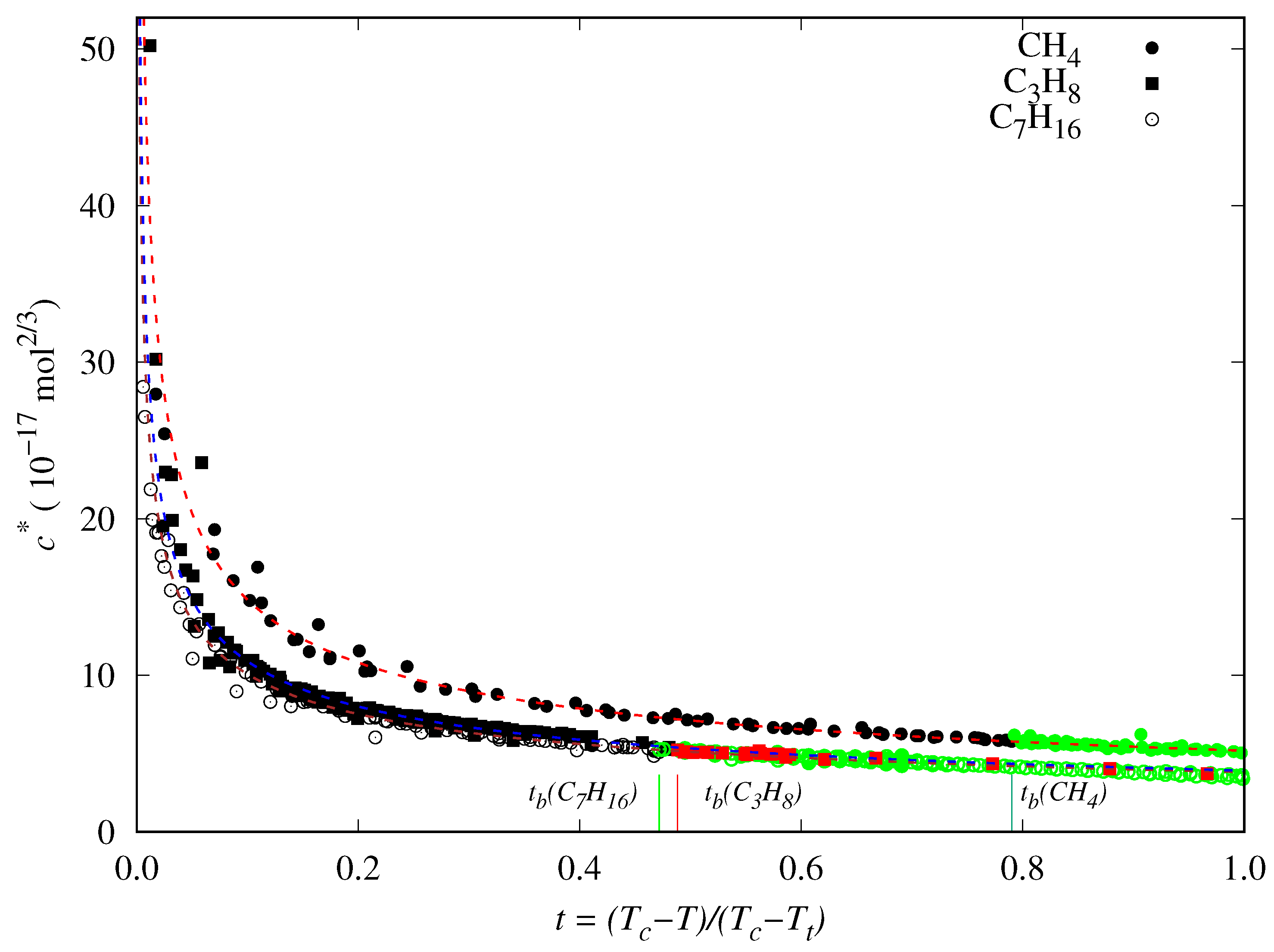
Some examples of the behavior of the reduced influence parameter versus the reduced temperature are shown in Figure 2. In particular, results for methane, n-butane, and n-heptane are displayed, which were calculated using the surface tension data previously selected and screened. Reduced boiling temperatures are marked as vertical lines. The chosen data at temperatures above the boiling point are shown in black, whereas those at lower temperatures are colored.
In a previous paper, we considered the dependence of c * versus t for several esters [49], and analyzing their behavior, we proposed a new correlation. We realize some common features by comparing those previous results for esters with those observed in Figure 2 for some n-alkanes. In particular:
i.
c * decreases almost linearly in the range [ t b , 1 ], so it could be fitted to a linear expression:
c * ( t ) = m 2 ( t 1 ) + m 1 ,
where m 2 < 0 is the slope and m 1 = c * ( 1 ) > 0 is the value of the reduced influence parameter at the triple point temperature.
ii.
Near the critical point ( t 0 ), c * tends to infinity. To reproduce this behavior, an analytical expression as the one proposed by Zuo and Stenby [33], has to be used:
c * ( t ) = A t n , with n < 0 ,
By combining both behaviours, Cachadiña et al. [49] have proposed a new analytical expression to calculate accurately the surface tension of esters:
c * ( t ) = m 0 ( t n 1 ) + m 1 .
They have shown that the value n = 0.392 can be considered a universal exponent and that it is related to the value for the critical exponent parameter associated with the density at the vapor-liquid equilibrium.
The results obtained in Ref. [49] show that, at least for esters, the accuracy of this expression is similar to the one from Zuo and Stenby, Equation (14). Even though they have the same number of adjustable coefficients, the new proposal is linear for m 0 and m 1 , so it is more straightforward to determine them when the reduced influence parameter is fitted using a least squares minimization method.
Nevertheless, when Zuo and Stenby, Equation (14), or Cachadiña et al. , Equation (15) correlations are applied to fluids for which surface tension data are available in a wide low-temperature range and they are linear with the reduced temperature, as it is the case of a majority of n-alkanes, the obtained results are not so accurate.
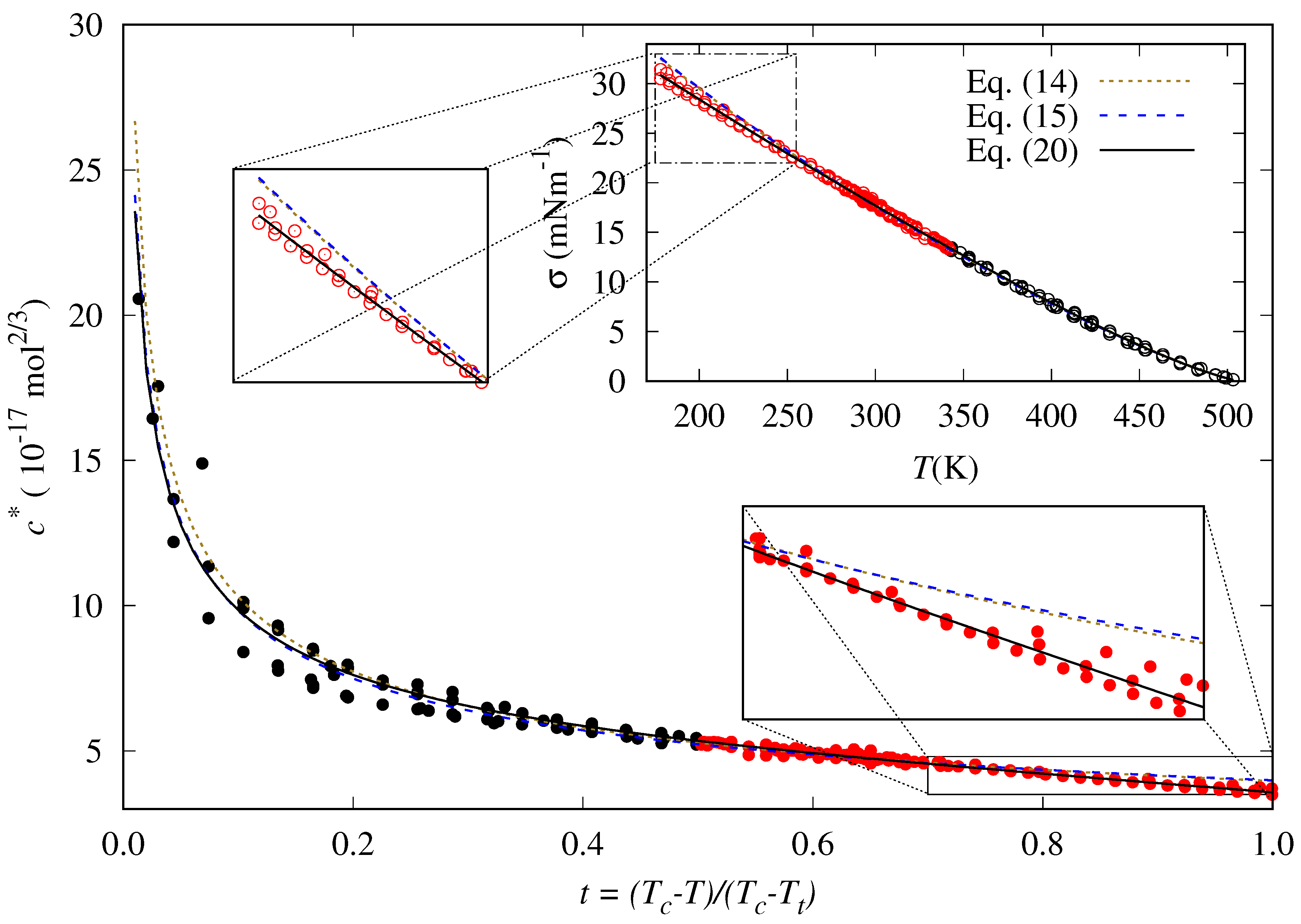
As shown in Figure 3, in the case of n-hexane, for instance, the Equations (14) and (15) cannot reproduce accurately the behavior of the reduced influence parameter at low temperatures ( T < 250 K or t > 0.7 , approximately), and consequently, the surface tension values are overestimated. These two correlations cannot appropriately describe the data trend in this temperature range.
The observed behavior suggests that the second derivative of the reduced influence parameter should be near zero in the temperature range from the triple point to normal boiling point temperatures. That is:
d 2 c * d t 2 0 t b > t 1 ,
It is easy to show that neither Zuo and Stenby or Cachadiña et al. correlations fulfill this condition, as their second derivatives at t = 1 are A n ( n 1 ) and m 0 n ( n 1 ) , respectively.
This work aims to propose a correction term, η ( t ) , to the expression proposed by Cachadiña et al. , Equation (15), to accurately reproduce the behavior of the reduced influence parameter at low temperatures. Thus, the new proposal is written as:
c * ( t ) = m 0 ( t n 1 ) + m 1 + η ( t ) .
with the following conditions at t = 1 (triple point temperature):
c * ( 1 ) = m 1 η ( 1 ) = 0 , d c * ( t ) d t | t = 1 = m 2 d η ( t ) d t | t = 1 = m 2 n m 0 , d 2 c * ( t ) d t 2 | t = 1 = 0 d 2 η ( t ) d t 2 | t = 1 = m 0 n ( n 1 ) .
The simplest analytical form of η ( t ) is the second order polynomial:
η ( t ) = q 0 + q 1 ( t 1 ) + q 2 ( t 1 ) 2 ,
that leads to the following analytical expression for the reduced influence parameter:
c * ( t ) = m 0 ( t n 1 ) + m 1 + ( m 2 n m 0 ) ( t 1 ) 1 2 n ( n 1 ) m 0 ( t 1 ) 2 ,
where the value n = 0.392 is fixed accordingly to the proposal of Cachadiña et al. [49]. As required in Equation (18), m 1 and m 2 are, respectively, the value and the slope of the reduced influence parameter at the triple point temperature ( t = 1 ).
It is essential to consider that the coefficients m 0 , m 1 , and m 2 must fulfill some constraints: since the influence parameter is positive, both m 0 and m 1 must be positive. On the other hand, at lower temperatures, it is observed that the reduced influence parameter follows a straight line with a negative slope [48], so m 2 has to be negative.
It is worth noting that when m 0 = 0 , Equation (20) results in:
c * ( t ) = m 1 + m 2 ( t 1 ) ,
which is equivalent to the linear correlation proposed by Miqueu et al. [48]:
c * = q 1 t + q 0 ,
when using PR EoS with volume translation [112]. In Equation (22), q 0 and q 1 are adjustable coefficients, and t = 1 T / T c is a reduced temperature. The following relations between q 0 , q 1 , m 0 , and m 1 are obtained easily when comparing (21) and (22):
q 0 = m 1 m 2 .
q 1 = m 2 1 T t T c .
.
Once the analytical expression given in Equation (20) has been proposed, the values of the coefficients must be determined. This work considers a comprehensive dataset of surface tension values for 32 n-alkanes, and the results are shown and discussed in the next section.

5. Results and Discussion

The values of coefficients m 0 , m 1 , and m 2 in Equation (20) have been obtained by minimizing the mean absolute percentage deviation ( MAPD f i t ) of every fluid:
MAPD f i t ( % ) = 100 N f i t i = 1 N f i t σ i σ D G T ( T i ) σ i ,
being N f i t the number of surface tension values selected for fitting that fluid. σ i is the surface tension datum at temperature T i , and σ D G T ( T i ) the calculated surface tension at the same temperature.
As it is well-known, the surface tension must be precisely zero at the critical point, and it takes values very near zero at temperatures closer to it. Consequently, no matter the model used, the absolute deviations will take low values. In contrast, the percentage deviations will be higher than those obtained at temperatures far from the critical point [49]. Thus, the data at temperatures closer to T c ( t 0 ) will significantly contribute to the sum in (25) and could bias the fitting results. To avoid this, only data with t 0.02 were considered in the fitting process. Also, those data from Sugden’s correlation are included. Thus, the specific correlation coefficients were determined with N f i t = 2652 out of the N = 2680 available data.
As the objective function Equation (25) is not linear in the adjustable coefficients, a careful choice of its initial values has to be taken. Since the expression for c * in Equation (20) is linear in m i ( i = 0 , 1 , 2 ), the initial values for m i have been obtained by using a linear least squares method [113] using the following merit function:
S 2 = i = 1 N f i t c i * c m o d e l * ( t i ) c i * 2 .
Then, these values were used in Powell’s minimization algorithm [113] to find the minimum MAPD f i t (Equation (25)). To prevent Powell’s method from falling into a local minimum, random displacements were given to the best values for the adjustable coefficients found, and then a new minimization was carried out. After 50 random displacement iterations, the coefficients of the lowest MAPD f i t found are saved.
The statistical figures discussed in the next two sections are defined for each fluid, considering all the available data (N) and regardless of the number of data fitted (see Table 1). The mean absolute percentage deviation (MAPD):
MAPD ( % ) = 100 N i = 1 N σ i σ D G T ( T i ) σ i ,
the mean deviation (MD):
MD ( % ) = 100 N i = 1 N σ D G T ( T i ) σ i σ i ,
and the maximum absolute percentage deviation ( PD m ):
PD m = 100 · max i = 1 , , N σ i σ D G T ( T i ) σ i .
In the following subsections, the values for the adjustable coefficients of the specific model for each fluid are given, and their variation is analyzed. Then, the accuracy of these proposed correlations is analyzed. Finally, the last section is devoted to proposing a new general correlation valid for all the considered n-alkanes and studying its results.

5.1. Adjustable Coefficients For The Specific Correlation

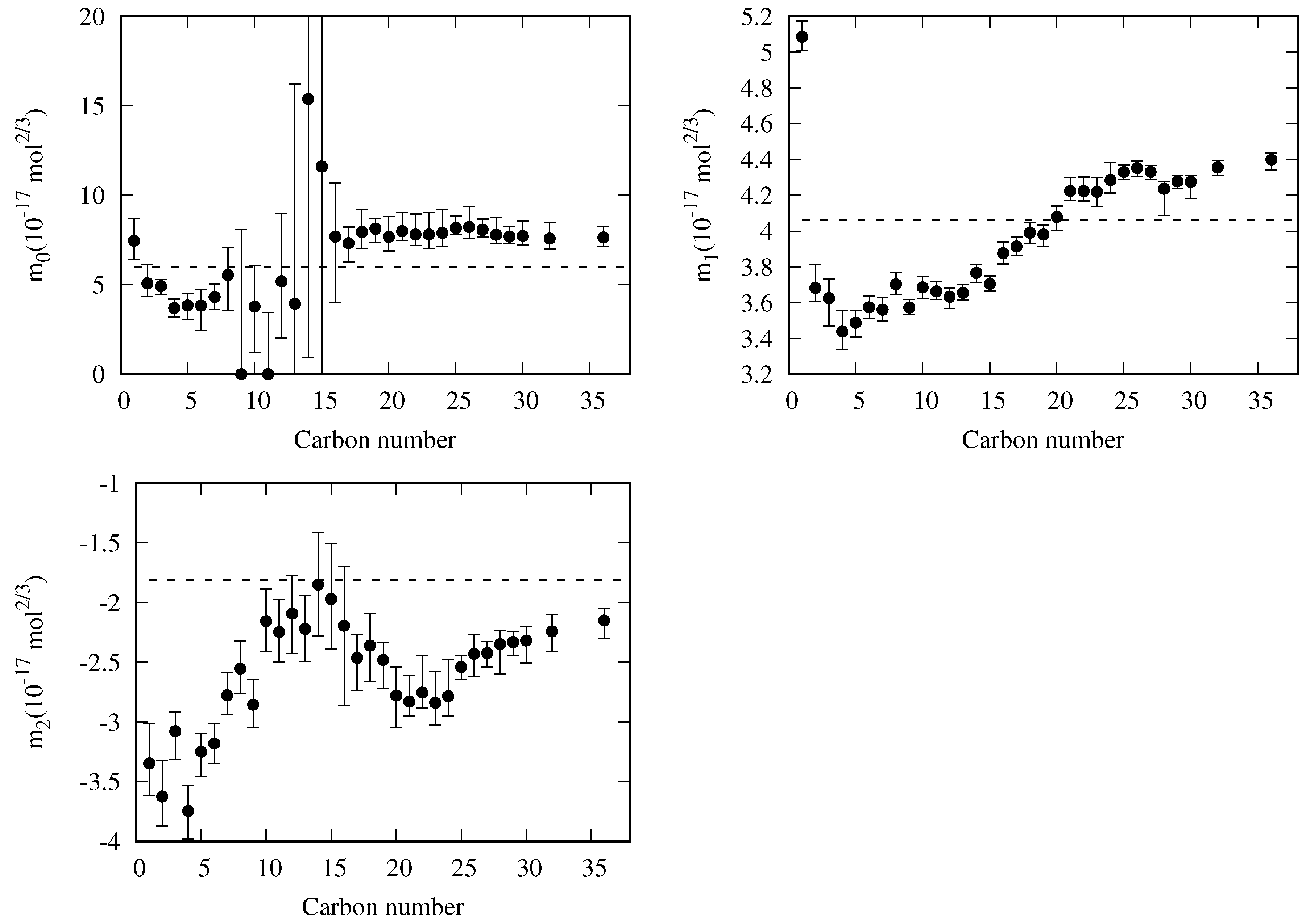
As a first step to study whether a global correlation for the m i can be finally found, it is interesting to evaluate how the variation of the value of a given m i coefficient influences in the resulting MAPD. Thus, we have calculated the displacements Δ m i + and Δ m i that increase the MAPD value by 0.25%, keeping the other coefficients fixed. In Figure 4, the values of m 0 , m 1 , and m 2 are plotted as a function of the carbon number of each n-alkane, with the vertical bars indicating the ranges m i Δ m i and m i + Δ m i + . The numerical values of m i and the min ( Δ m i , Δ m i + ) , MAPD, maximum percentage deviation ( PD m ), and reduced temperature t PDm where the maximum deviation is reached, are compiled in Table 1.
It is noteworthy that n-nonane and n-undecane have their m 0 = 0 . This value results from the lack of data at temperatures above the normal boiling point (see Figure 1). Thus, when plotting the reduced influence parameter versus the reduced temperature for both fluids, the observed values follow a straight line with no appreciable curvature. Since the constraint m 0 0 is set in the fitting process, the result is the analytical expression mentioned in Equation (21). As shown in Table 1, for n-nonane and n-undecane m 0 can be risen up to 8.1 and 3.4 × 10 17 mol 2 / 3 , respectively, without increasing the resulting MAPD by more than 0.25%.
The error bars associated with the obtained values for the adjustable coefficients of these fluids suggest that there is some room to choose other values for the adjustable coefficients that lead to a non-zero m 0 value, which could lead to a suitable extrapolation to higher temperatures, which will be discussed in the next section.
For the other n-alkanes considered, the m 0 values decrease with the carbon number down to n-butane. The trend for the heavier fluids seems to be compatible with a plateau starting from the n-alkane with 16 carbons. Unfortunately, this observation is biased by the fact that the m 0 values are determined mainly by the high-temperature range, and for these fluids, all the available data in this range (see Figure 1) are the predictions made by the DIPPR project [109] using Sugden’s correlation.
The narrow bars for m 1 observed for all the n-alkanes in Figure 4 are related to the role that m 1 plays in the proposed correlation, as the surface tension values at lower temperatures mainly determine it. As there is a high data availability in the temperature range between the triple and normal boiling points, a slight variation of m 1 will lead to a considerable change in the predicted values for this range, and so, the observed narrow bars are expected.
The highest value for m 1 is obtained for methane, decreasing to n-butane and increasing for higher n-alkanes. On the other hand, for carbon number higher than 25, the value of m 1 could be regarded as a constant.
Coefficient m 2 is related to the slope of the reduced influence parameter at the triple point temperature. The tendency observed in Figure 4 is almost a linear behavior up to carbon number 15. For higher carbon numbers, the observed behavior could be due to the DIPPR predictions, so we need to take them with some caution.
Finally, it is necessary to stress that the m i values reported in this work can be used to match the observed behavior for n-alkanes with a high degree of accuracy. Nevertheless, it has to be clear that, for carbon number greater than 15, the given correlation will reproduce mostly the DIPPR predictions. When new data becomes available for one of these fluids, a new fit is expected to yield a certain change in the corresponding m 0 and m 2 values.

5.2. Accuracy Of The Proposed Specific Model

By using Equation (20) and the values for the adjustable coefficients obtained for each fluid, the MAPDs, MDs, and PD m were calculated. Results are shown in Table 1 (remind that these values are obtained with all the data available for each fluid and not only with the considered in the fit).
The resulting deviation values are of the same order as those reported by Mulero et al. for n-alkanes [73] when using the Guggenheim-Katayama correlation with two, four, or six fitting coefficients for each n-alkane. For example, making a comparison for methane, the use of Guggenheim-Katayama correlation with four adjustable coefficients leads to an MAPD = 0.93% and PD m = 9.68% [73], while using the here-proposed correlation with three adjustable coefficients the obtained deviations are MAPD = 0.97% and PD m = 8.5%.
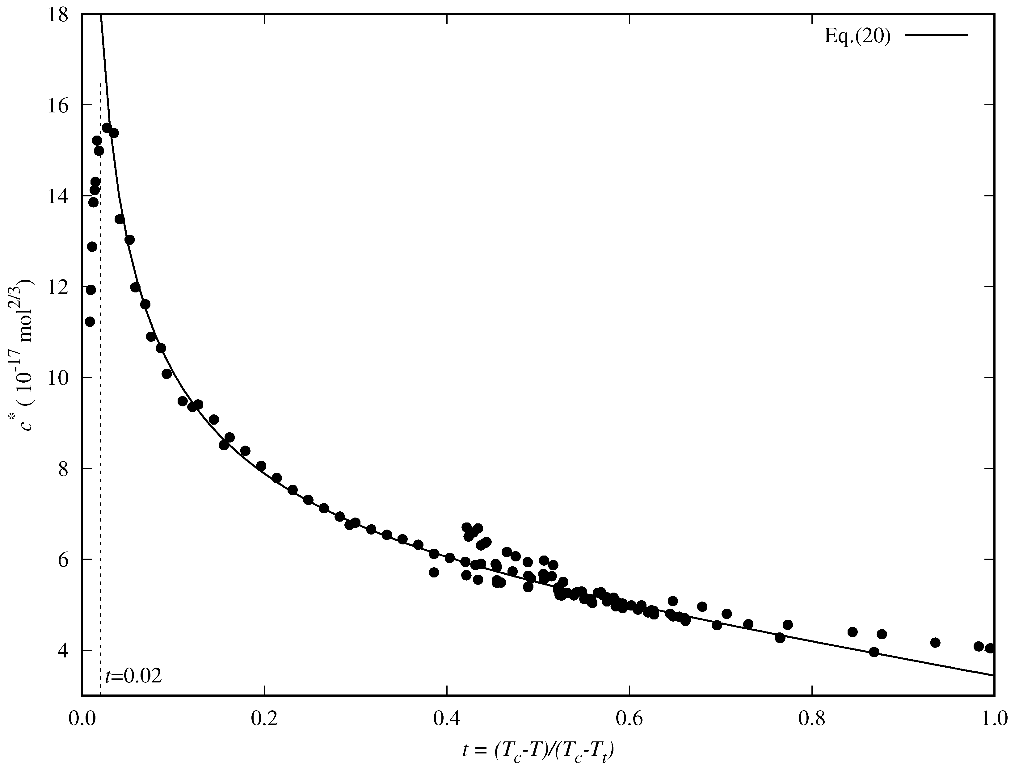
The highest PD m value found here, 48.9%, is obtained for n-butane, while Mulero et al. reported a PD m value of 11.70% using six adjustable coefficients for this same fluid [73]. This highest PD m value is located near the critical point temperature ( t PD m = 0.01 ). As shown in Figure 5, this is due to the anomalous behavior of the reduced influence parameter observed for this fluid, which decreases sharply at temperatures t 0.02 . Consequently, a high disagreement between the correlation predicted data and the surface tension values is obtained in this temperature range, i.e., near the critical point. Note that for the first eight n-alkanes, the results for t < 0.02 are extrapolated values, and the PDm of five out of the eight first n-alkanes are located in this range.
As the surface tension values near the critical point are subject to high uncertainty, it is interesting to check what values for MAPD and PD m are obtained when a narrower temperature range is considered, but keeping the m i values compiled in Table 1.
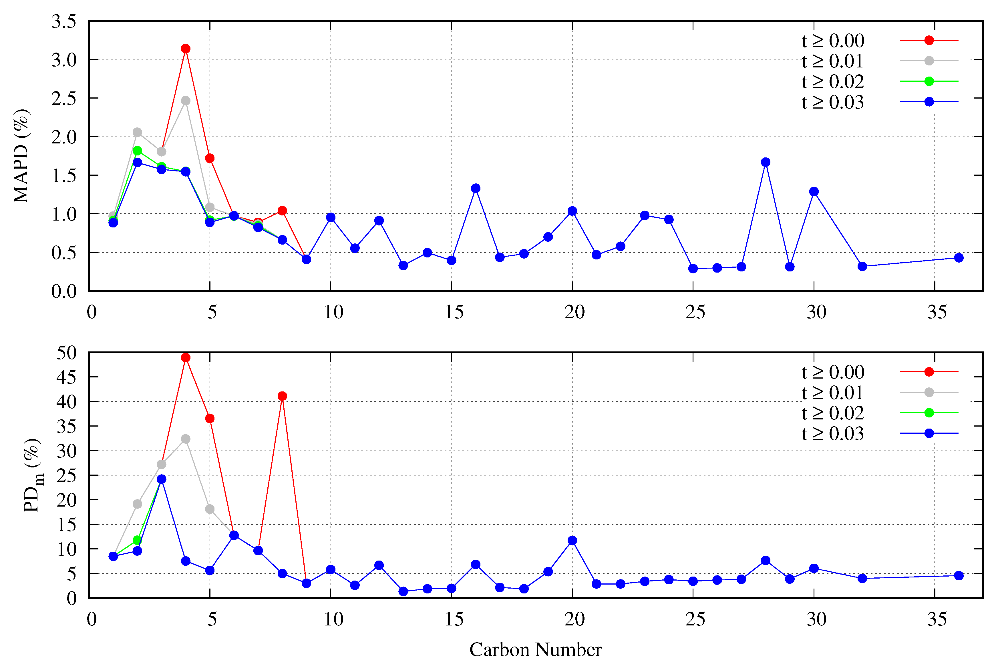
As shown in Figure 6, the maximum value of 48.9% for n-butane is lowered down to 7.54% when only data with t 0.02 are considered. No significant reduction is obtained when t 0.03 , where only the PD m of ethane is affected. On the other hand, the MAPDs calculated in the range t 0.02 yield values below 2% in all cases, a reasonable value since their origin is due to the disagreement between the different sources of surface tension data rather than the analytical form of the proposed correlations.

5.3. General Correlation

The lack of experimental data above the normal boiling point, especially for the higher n-alkanes (see Figure 1), suggests the importance of the development of a general correlation applicable to all of them and that permits to obtain predicted values. The DIPPR project, for example, includes in its database some predicted data based on the application of Sugden’s correlation [110]. This correlation establishes a relation between surface tension and the 4 th power of the liquid and vapor density difference. This data should not be considered when developing a new general correlation.
Before obtaining a general correlation, we need to make some considerations:
  • The DIPPR data predicted using Sugden’s correlation will not be considered in the new global correlation, and only data in the range t 0.02 will be considered in the coefficient determination of the global correlation. The number of available data and fitting data for each fluid are compiled in Table 5.
  • There are some fluids (see Figure 1) for which a considerable number of fitting data are available (i.e., n-heptane and n-hexane with 357 and 269 data, respectively), whereas in other cases the number of data is one (n-hexatriacontane and others). To have a suitable general correlation not biased by the data availability, the adjustable coefficients will be obtained by minimizing the overall mean absolute percentage deviation ( OMAPD f i t ), defined as:
    OMAPD f i t ( % ) = 1 N f l u i d s k = 1 N f l u i d s MAPD f i t , k ,
    where MAPD f i t , k is the mean absolute percentage deviation of the fluid k, defined in Equation (25), but taking N f i t from Table 5, and with N f l u i d s the number of fluids (32 in these case). Thus, the coefficients of the general correlation will be determined with N f i t = 2427 data, with a weighing scheme depending on the fitting data of each fluid.
As a first approximation, a general correlation where all the m i coefficients are regarded as constant is explored. The coefficient values that minimized the OMAPD f i t , defined in Equation (30), are: m 0 = 5.983 , m 1 = 4.060 , and m 2 = 1.810 (all of them in 10 17 mol 2 / 3 units). These values, which are shown as dashed lines in Figure 4, yield the OMAPDs of the whole and fitting data sets of 4.38% and 3.35%, respectively (see Table 2). When considering the overall mean deviation for the whole and fitting sets, defined as:
OMD whole / f i t i n g ( % ) = 1 N f l u i d k = 1 N f l u i d MD k , whole / f i t t i n g
the values obtained OMD whole = 1.38 % and OMD f i t = 0.53 % , respectively. This shows that the surface tension is under-predicted in most fluids (i.e., MD is negative in most cases).
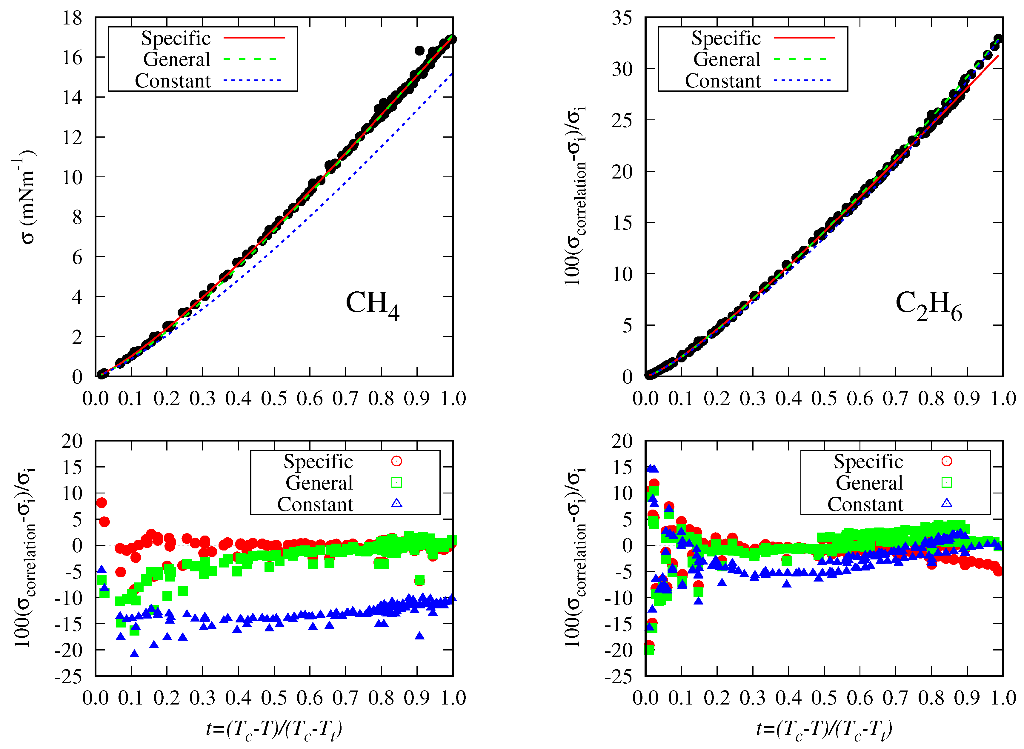
As expected, this most straightforward correlation gives poor results when compared to the specific correlations given in Table 1, but these results are not so bad when considering the difference in the number fitting coefficients: 96 vs. 3. Indeed, the MAPD f i t values are less than 5.0% with the only exception of methane (see Figure 7), for which the largest MAPD and MD deviations are found. In other fluids, i.e., ethane (see Figure 7), the constant correlation yields reasonable results despite the low number of fitting coefficients used.
It is crucial to take into account that, in some cases, the deviations are not only due to the behavior of the model but also to the disagreement between the data for the surface tension obtained by different authors for the same fluid and temperature range (the previous Figs. show several examples). As expected, despite the absolute deviations being low at high temperatures (t near zero), the percentage deviations are high, as is the case of any other models or correlations [73].
In addition, it must be pointed out that a new coefficient fit, excluding methane, could lead to lower MAPDs for the other n-alkanes. In this way, two 3-coefficient sets (3 for methane and 3 for the other n-alkanes) could be proposed, but, as is shown below, it is possible to find a 6-coefficient general correlation depending on some fluid parameter and giving low MAPDs with good extrapolation features.
Table 2. Statistical figures of the general correlation when all the m i are taken as constants (no fluid dependence). CN is the carbon number, N the number of data, MAPD the mean absolute percentage deviation, MD the mean deviation, PD m the maximum absolute percentage deviation, and t PDm is the reduced temperature of the maximum percentage deviation. The subscript f i t is added for those figures calculated with the fitting set (2427 values). The other results are for the whole data set (2681 values). The fitting parameters are m 0 = 5 . 983 , m 1 = 4 . 060 , and m 2 = 1 . 810 (in 10 17 mol 2 / 3 units).
CN N / N f i t MAPD/ MAPD f i t MD/ MD f i t PD m / PD m f i t t PDm / t PDm f i t
(%) (%) (%)
1 127/126 12.99/13.05 -12.99/-13.05 +20.95/+20.95 0.11/ 0.11
2 163/160 3.48/3.28 -2.33/-2.29 15.80/14.41 0.01/ 0.02
3 193/191 2.14/2.00 -0.49/-0.34 22.59/22.10 0.01/ 0.06
4 126/118 5.42/2.59 2.35/-0.70 75.48/+15.04 0.01/ 0.03
5 149/143 3.53/2.06 3.00/ 1.51 62.01/17.12 0.01/ 0.02
6 270/269 1.82/1.76 1.20/ 1.14 17.35/16.20 0.01/ 0.04
7 363/357 2.94/2.71 2.90/ 2.68 20.39/17.97 0.01/ 0.05
8 196/194 2.41/2.00 2.17/ 1.76 45.07/5.72 0.01/ 1.00
9 78 3.52 3.52 6.93 0.99
10 149 3.80 3.74 9.71 0.12
11 60 4.36 4.36 10.43 0.30
12 100 4.98 4.98 12.18 0.91
13 48 4.30 4.30 5.86 0.99
14 49 3.60 3.39 5.72 0.97
15 40 4.19 4.19 5.37 0.95
16 127/117 2.40/2.31 1.52/ 1.90 7.31/7.17 0.08/ 1.00
17 44/ 34 1.56/1.06 -0.13/ 0.80 7.16/2.15 0.07/ 0.78
18 39/ 29 1.57/0.55 -0.92/ 0.34 9.37/1.40 0.07/ 1.00
19 23/ 12 2.85/1.20 -2.49/-0.51 10.41/10.20 0.07/ 0.34
20 38/ 25 2.89/1.43 -2.78/-1.26 17.69/17.69 0.33/ 0.33
21 28/ 14 5.86/4.78 -5.86/-4.78 14.00/7.35 0.07/ 0.49
22 32/ 19 5.16/4.05 -5.16/-4.05 13.18/6.99 0.07/ 0.54
23 36/ 22 5.05/3.74 -5.05/-3.74 13.93/6.97 0.06/ 0.52
24 36/ 22 5.60/4.43 -5.56/-4.36 14.37/7.22 0.06/ 0.61
25 15/ 1 6.92/3.48 -6.92/-3.48 14.70/3.48 0.06/ 0.95
26 31/ 19 5.40/3.96 -5.40/-3.96 14.97/4.45 0.06/ 0.81
27 16/ 1 6.45/3.32 -6.45/-3.32 14.52/3.32 0.06/ 0.96
28 24/ 9 4.42/2.57 -3.35/ 0.29 13.13/4.23 0.06/ 0.78
29 16/ 1 5.41/2.60 -5.41/-2.60 12.95/2.60 0.06/ 0.97
30 22/ 7 4.64/2.57 -3.91/-0.30 13.07/4.01 0.06/ 0.55
32 25/ 12 4.92/3.64 -4.92/-3.64 12.61/4.23 0.06/ 0.85
36 18/ 1 5.67/3.48 -5.67/-3.48 13.36/3.48 0.06/ 1.00
- 2681/2427 75.48/22.10
N f l u i d OMAPD/ OMD/
OMAPD f i t OMD f i t
32 4.38/3.35 -1.38/-0.53
One of the present work aims is to give a simple general correlation for the surface tension of n-alkanes that could correlate the available surface tension data with high accuracy and having good extrapolation capability. That kind of correlation is usually written as a function of some fluid properties with fixed values, such as the critical pressure, acentric factor, or others [114]. In this work, we have considered all the properties in Table 3, whose values were obtained from the DIPPR [109] database. Nevertheless, it is worth noting that some of the fluid properties in the DIPPR database are also predicted, and it is especially true for the higher n-alkanes, so the predictions made for these fluids have to be taken cautiously.
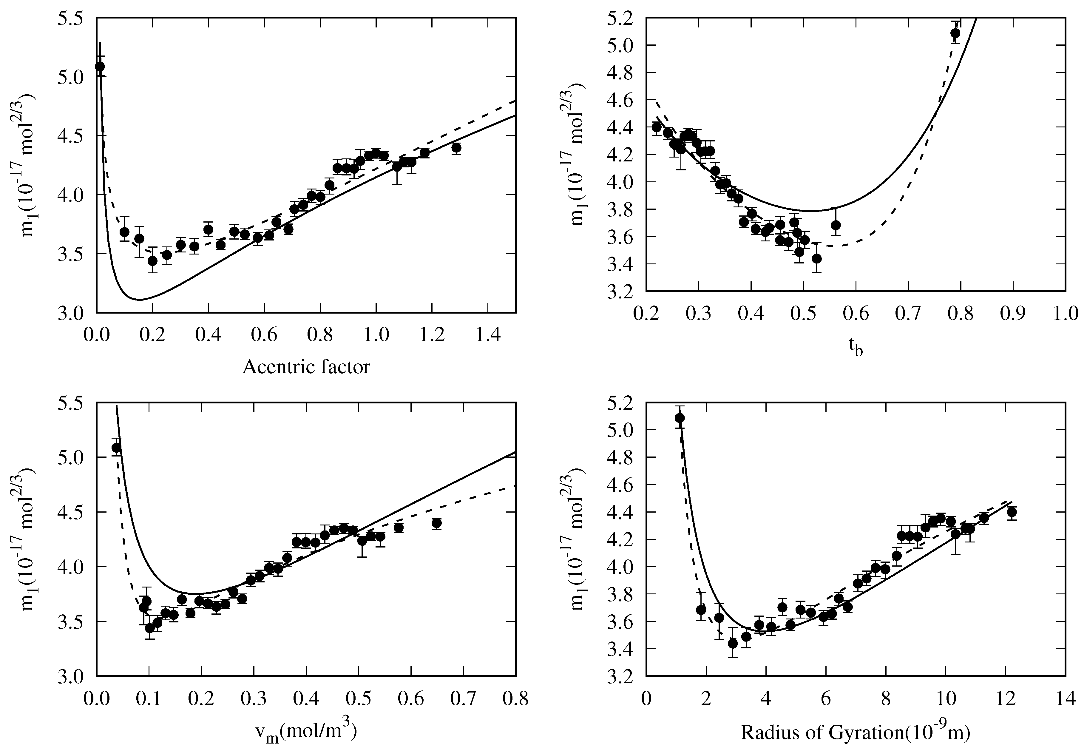
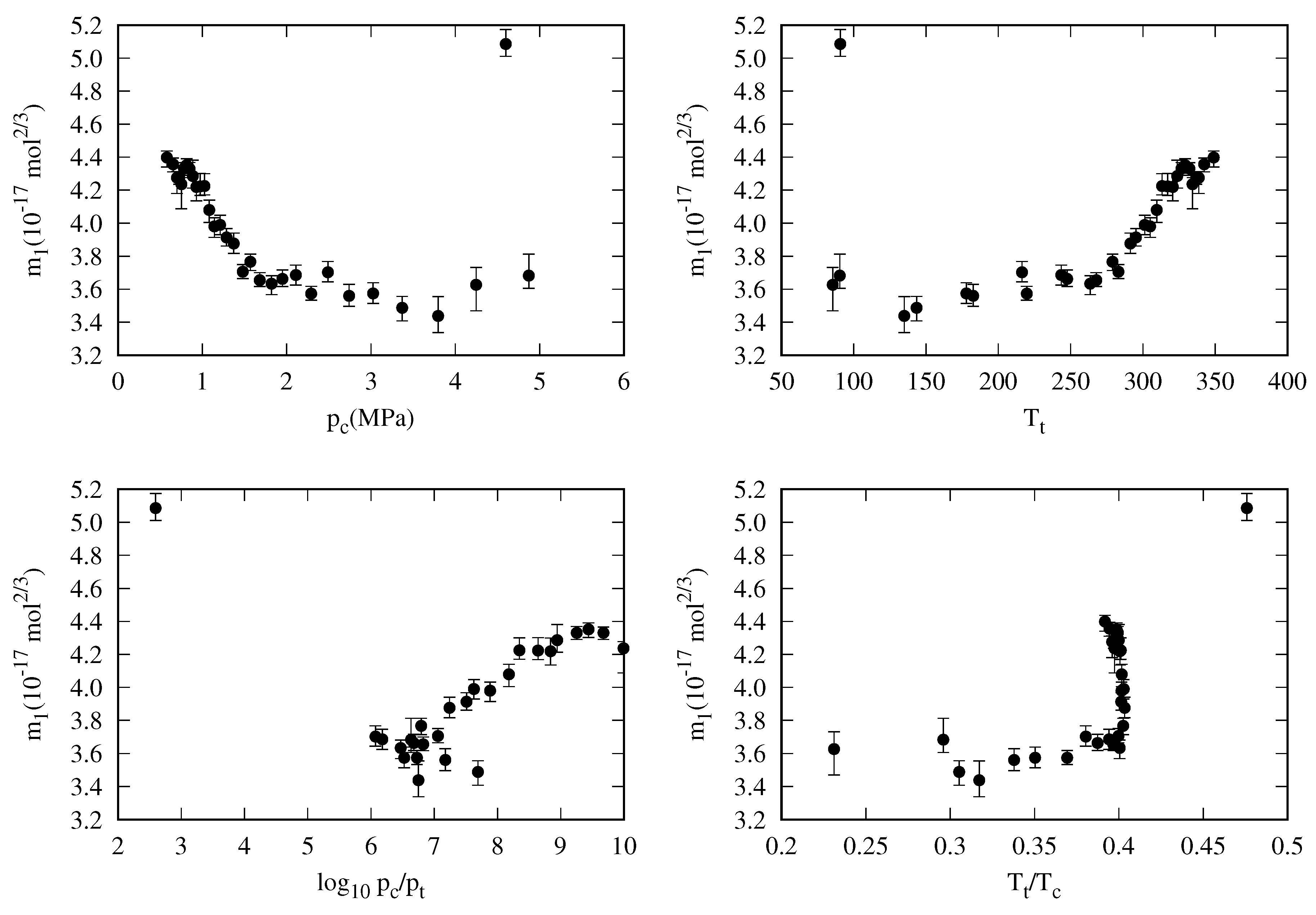
We will first explore the m 1 dependence from the fluid properties, as this is the most sensitive coefficient, i.e., a slight deviation in its values leads to a significant increase of the MAPD. When plotting m 1 versus the fluid properties listed in Table 3, one can see that there are some well (see Figure 8) and badly (see Figure 9) behaved candidates for a correlation. Other, as the dipole moment ( μ ), cannot be used as it has the same value (zero) for all the n-alkanes family.
For those properties that are well-behaved, the following functional dependency is proposed here:
m 1 ( x ) = a 1 x n 1 + a 2 x n 2 , ( n 1 > 0 , n 2 > 0 ) ,
where x is the chosen fluid property. In Figure 8, the dashed lines are the fits of the m 1 values to Equation (32) obtained using a least squares method.
Table 3. Fluid properties considered in the possible m i correlations.
Name Symbol Units
0 No dependency (constant) - -
1 Critical Pressure p c Pa
2 Critical Temperature T c K
3 Acentric factor ω -
4 Critical compressibility factor Z c -
5 Critical Volume v c L mol 1
6 Melting temperature T f K
7 Triple point temperature T t K
8 Normal boiling point temperature T b K
9 Logarithmic ratio between p c and p t log 10 ( p c / p t ) -
10 Liquid molar volume at 298.15 K and 101325 Pa v m L mol 1
11 Radius of Gyration RG 10 9 m
12 Dipole moment μ Cm
13 Molar weight M w kg kmol 1
14 Reduced triple point temperature T t / T c -
15 Reduced normal boiling temperature T b / T c -
16 Pseudo compressibility factor p c v m / ( R T b ) -
17 Reduced boiling temperature t b = ( T c T b ) / ( T c T t ) -
To keep the number of fitting parameters as low as possible, we have considered that m 0 and m 2 are constants, and m 1 is correlated with the chosen fluid property (x) as shown in Equation (32). Then, the number of fitting coefficients for c m o d e l * will be 6, that is { m 0 , a 1 , n 1 , a 2 , n 2 m 1 , m 2 } . The fitting coefficients have been obtained by minimizing the OMAPD f i t of the surface tension data, defined in Equation (30). The initial values for m 0 and m 2 are the ones previously determined in the constant model, whereas the others ( a 1 , n 1 , a 2 , n 2 ) are the corresponding ones to the functions in dashed lines in Figure 8, that have been obtained with a least squares method to the m 1 data. The minimization procedure is the same as that used for the specific correlation fitting.
As shown in Figure 8, the dashed lines of the m 1 fits are in better agreement than the solid lines corresponding to the global fit. This is an expected result, provided that in the global fit, the coefficients m 0 and m 2 have been regarded as a constant for all the fluids, and a small deviation in the m 1 correlation is needed to fulfill this requirement.
The error bars shown in Figure 8 represent the variation range of the corresponding m 1 values to increase the MAPD in a 0.25% keeping m 0 and m 2 fixed. For example, in the case of the radius of gyration, the figure shows that the disagreement between the general correlation (solid lines) and the m 1 points should increase the MAPD of each fluid by about 0.5% from the specific correlation (dashed lines).
Table 4 summarized the coefficients and the statistical deviations of the correlations for the parameter m 1 when correlating with different physical properties. It can be seen that the best correlation is found when the radius of gyration is used ( OMAPD f i t =1.78%), followed by v c ( OMAPD f i t =1.94%) and v m ( OMAPD f i t =1.99%). When the whole set is considered in evaluating the OMAPD w h o l e , the deviations are 2.26%, 2.52%, and 2.78%, respectively.
Table 4. Adjustable coefficients and statistical deviations for different physical properties considered in the correlation for m 1 = a 1 x n 1 + a 2 x n 2 , where x is the chosen property.
Adjustable coefficients RG v c v m t b ω
m 0 ( 10 17 mol 2 / 3 ) 5.01227 4.91156 5.37325 6.48294 4.99955
a 1 ( 10 17 mol 2 / 3 ) 4.40431 1.09159 0.662073 3.03929 0.625431
n 1 0.885059 0.53364 0.595946 0.254804 0.452929
a 2 ( 10 17 mol 2 / 3 ) 1.08825 2.68771 4.84453 5.0875 3.52179
n 2 0.519495 0.401163 0.542305 4.98139 0.405698
m 2 ( 10 17 mol 2 / 3 ) -2.92951 -2.6442 -2.05972 -2.20715 -3.45186
Statistical figures for the fitting set
OMAPD f i t (%) 1.78 1.94 1.99 2.16 2.18
MD f i t (%) 0.04 -0.02 -0.13 0.16 0.24
PDm f i t (%) 23.93 24.37 23.76 21.44 24.35
Statistical figures for the whole set
OMAPD(%) 2.26 2.52 2.78 2.68 2.57
MD(%) -0.45 -0.79 -1.20 -0.37 0.11
PDm(%) 65.02 63.50 68.36 81.76 64.95
The low deviations obtained when using different well-behaved fluid properties suggest that the analytical form of the reduced influence parameter and the choice of the parameters are sounded. Thus, it seems natural to have a fixed parameter ( m 0 ) governing the high-temperature range, another fixed parameter m 2 governing the rate of change with temperature of the surface tension, and other fluid-dependent properties related to the surface tension at the triple point temperature.
Although the deviations found when using different fluid parameters are very similar, it is quite appealing that the three lowest deviations are related to geometrical fluid properties: radius of gyration, critical volume, and liquid molar volume at 298.15 K and 101325 Pa.
The radius of gyration is related to the molecule’s shape, defined as the distance from the center of mass that a particle with the same mass as the molecule will lead to the same molecule’s momentum of inertia [109]. This property has been used by other authors in the development of correlations for the surface tension of ketones, silanes, and carboxilic acids [115,116,117], or the viscosity of silanes [118]. Then, it can be considered an adequate and useful input property for the correlation of fluid surface tension.
Table 5 shows detailed information on the number of data, fitted or not fitted, and the statistical deviations for each fluid when using the radius of gyration as input property. When considering the whole data set, all the MAPDs are below 4%, with the exception of n-butane, and they are below 3% (except for n-triacontane) for the fitting set.
Although we have included figures of surface tension and the correlations studied using the radius of gyration for all the n-alkanes in the supplementary material, it is worthwhile to briefly discuss the results obtained for a few selected fluids.
Figure 7 shows that for methane, the general correlation deviates from the surface tension data in the high-temperature range. For ethane, there are two data trends at lower temperatures, and the general correlation follows a different trend than the specific one. It can also be appreciated that the deviations in the high-temperature range are mainly due to the disagreement between data and not by the correlation performance.
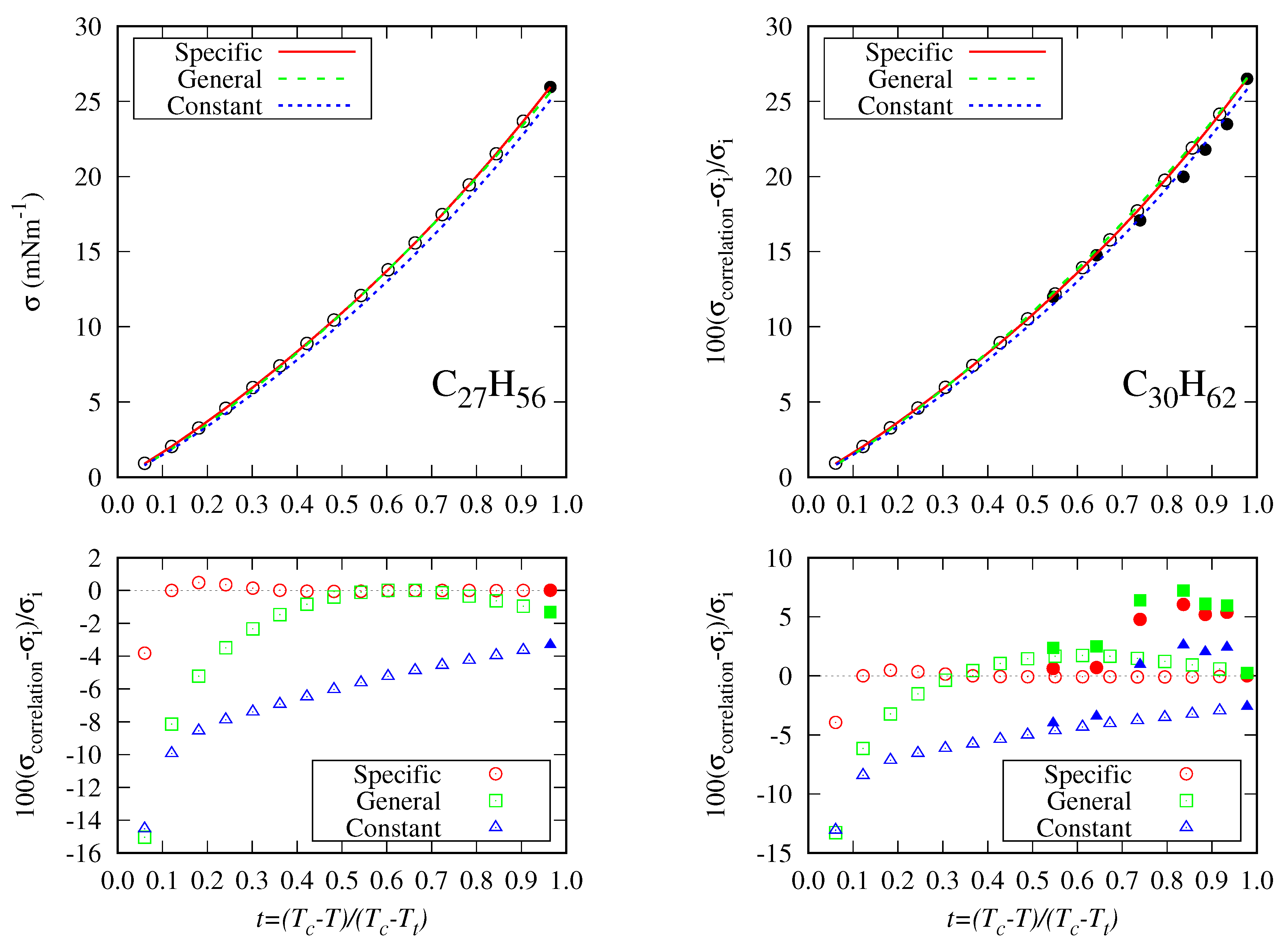
On the other hand, as an example for those fluids with few data in the fitting set, Figure 10 shows the surface tension data for n-heptacosane (one datum) and n-triacontane (seven data). As can be seen, the specific model behaves very well but deviates about 4% at higher temperatures. As expected, the general correlation behaves better than the constant model for both fluids. The data dispersion in the lower temperature range between the DIPPR predicted data and the fitting set can be appreciated in n-triacontane.
Table 5. Statistical figures of the global correlation when m 0 = 5 . 012 , m 2 = 2 . 92951 and m 1 = 4 . 40431 x 0 . 8851 + 1 . 08825 x 0 . 5195 (all in 10 17 mol 2 / 3 units), with x being the Radious of gyration. CN is the carbon number, N the number of data, MAPD the mean absolute percentage deviation, MD the mean deviation, PD m the maximum absolute percentage deviation, and t PDm is the reduced temperature of the maximum percentage deviation. The subscript f i t is added for those figures calculated with the fitting set.
CN N / N f i t MAPD/ MAPD f i t MD/ MD f i t PD m / PD m f i t t PDm / t PDm f i t
(%) (%) (%)
1 127/126 2.49/2.45 -2.20/-2.16 16.28/16.28 0.11/ 0.11
2 163/160 2.58/2.35 0.09/ 0.25 20.01/10.71 0.01/ 0.04
3 193/191 1.84/1.65 0.27/ 0.48 26.76/23.93 0.01/ 0.06
4 126/118 4.54/2.19 1.53/-1.02 65.02/10.03 0.01/ 0.03
5 149/143 2.42/1.25 1.75/ 0.54 51.44/11.26 0.01/ 0.02
6 270/269 1.72/1.69 -0.37/-0.41 12.64/12.64 0.07/ 0.07
7 363/357 1.36/1.22 0.96/ 0.81 13.96/13.96 0.05/ 0.05
8 196/194 1.40/1.08 -0.34/-0.68 35.68/4.47 0.01/ 0.19
9 78 0.54 0.38 3.76 0.54
10 149 1.55 0.97 8.52 0.12
11 60 1.77 1.77 11.63 0.30
12 100 2.37 2.34 7.96 0.91
13 48 1.66 1.66 4.26 0.69
14 49 0.96 0.61 3.76 0.72
15 40 1.67 1.67 4.58 0.74
16 127/117 1.77/1.73 -0.24/-0.09 8.64/7.67 0.08/ 0.46
17 44/ 34 1.15/0.84 -0.68/-0.39 8.56/2.20 0.07/ 0.78
18 39/ 29 1.50/1.08 -1.24/-0.74 10.54/2.65 0.07/ 0.99
19 23/ 12 2.06/1.44 -1.54/-0.64 11.62/7.08 0.07/ 0.34
20 38/ 25 2.48/1.97 -2.18/-1.52 14.55/14.55 0.33/ 0.33
21 28/ 14 3.80/2.81 -3.80/-2.81 14.97/3.63 0.07/ 0.49
22 32/ 19 3.15/2.48 -3.15/-2.48 13.98/3.32 0.07/ 0.63
23 36/ 22 2.79/1.90 -2.53/-1.47 14.82/3.23 0.06/ 0.64
24 36/ 22 3.02/2.20 -2.92/-2.04 15.08/3.94 0.06/ 0.80
25 15/ 1 3.64/2.25 -3.64/-2.25 15.32/2.25 0.06/ 0.95
26 31/ 19 2.32/1.39 -2.31/-1.36 15.59/2.09 0.06/ 0.93
27 16/ 1 2.53/1.31 -2.53/-1.31 15.04/1.31 0.06/ 0.96
28 24/ 9 3.33/4.91 1.05/ 4.91 13.58/8.81 0.06/ 0.78
29 16/ 1 2.22/0.07 -0.92/ 0.07 13.24/0.07 0.06/ 0.97
30 22/ 7 3.07/4.39 0.83/ 4.39 13.29/7.22 0.06/ 0.84
32 25/ 12 1.64/0.55 -0.11/ 0.55 12.66/0.97 0.06/ 0.87
36 18/ 1 2.88/1.30 0.45/ 1.30 13.31/1.30 0.06/ 1.00
Overall 2681/2427 65.02/23.93
N f l u i d OMAPD/ OMD/
OMAPD f i t OMD f i t
32 2.26/1.78 -0.45/0.04
The second and third lowest OMAPD are obtained when the critical and molar volumes are used as input properties. Nevertheless, the use of the molar volume rather than the critical one is recommended because it is more easily accessible from the experimental point of view.
The next input parameter with low OMAPD values is the reduced normal boiling temperature. Detailed information (similar to those in Table 5) for the readers interested in the performance of these fluid properties have been included as Supplementary Material.
Finally, in Table 4, the statistical deviations obtained when the acentric factor is used as a correlating property are listed. The advantage of using this parameter is that only the information of the triple point temperature ( T t ) is added to the information required for the PR78 EoS ( T c , p c , and ω ). The obtained OMAPD=2.57% of the global fit only increases in a 0.31% the value obtained when using the radius of gyration, and the mean deviation of the whole set is the lowest one compiled in Table 4. Detailed statistical information is included in the Supplementary Material.

6. Conclusions

In this paper, the data available for the surface tension of n-alkanes have been compiled and adequately selected. In particular, 2,681 data were selected for 32 fluids, and the data selected for each fluid ranged from 15 to 363. The available surface tension data show a high dispersion in some cases, as the values for the same fluid and temperature from different sources are usually in apparent disagreement. This can influence the results obtained when these data are used in a fitting procedure.
The Peng-Robinson-78 EoS has been selected to obtain the equilibrium vapor and liquid densities, and these properties were used as inputs in calculating the influence parameter according to the Density Gradient Theory. In particular, values for the reduced influence parameter were obtained for every fluid and temperature at which selected data for the surface tension were available.
A new analytical expression containing three adjustable coefficients ( m 0 , m 1 , and m 2 ) and a fixed exponent ( n = 0.392 ) is proposed to fit the reduced influence parameter values versus the reduced temperature. This correlation requires each fluid’s critical and triple point temperatures as input properties. Also, the analytical expression proposed holds the Miqueu et al. ( m 0 = 0 ) and Zuo and Stenby ( m 1 = m 0 , m 2 = 0 , n adjustable) correlations as particular cases.
The correlation coefficients are related to the reduced influence parameter: m 0 determines the behavior near the critical point temperature, m 1 is the value at the triple point temperature, and m 2 is the slope at the triple point temperature. The new proposal’s performance is comparable to the Guggenheim-Katayama correlation reported by other authors, so it can be considered an alternative.
From the analysis of the 96 fitting coefficients for all the fluids, it is observed that m 0 and m 2 can be fixed, and m 1 can be correlated with some fluid property, such as radius of gyration, molar volume, acentric factor, etc. Thus, a four-coefficient analytical expression for m 1 is proposed and fitted using the t 0.02 data without considering DIPPR data using Sugden’s correlation. The results show that the best results are obtained when the radius of gyration is used as an input parameter, and the results using critical point volume, molar volume, and other parameters are also good alternatives.
A new general correlation, containing six adjustable coefficients, can be used as a predictive tool to populate those temperature ranges for which there are no available data.
New studies will focus on the role of m 0 and m 2 in addition to the radius of gyration as an input property for other fluid families. Also, the extension of the proposed correlation to mixtures containing n-alkanes will be evaluated in future works.

Author Contributions

I.C. Conceptualization, methodology, software, writing, editing; A.H. writing, review, editing; A.M. Data curation, review, and editing.

Acknowledgments

I.C. and A.M. thank the financial support received from the “Junta de Extremadura” and "Programa FEDER Extremadura 2021-2027" of the European Union (European Regional Development Fund) through project GR24101. A.H. acknowledges the economic support given by the UCSC.

Conflicts of Interest

The authors declare no conflicts of interest.

References

  1. Adamson, A.; Gast, A. Physical Chemistry of Surfaces; Interscience publishers: New York, 1967; Vol. 150. [Google Scholar]
  2. Myers, D. Surfaces, Interfaces, and Colloids: Principles and Applications; John Wiley & Sons, Inc., 1999.
  3. Liu, H. Science and Engineering of Droplets: Fundamentals and Applications; Noyes Publications, 2000.
  4. Hartland, S. Surface and Interfacial Tension: Measurement, Theory and Applications; Marcel Dekker, 2004.
  5. Schramm, L.L. Emulsions, foams, and suspensions: Fundamentals and applications; John Wiley & Sons, 2006.
  6. Neumann, A.W.; David, R.; Zuo, Y. Applied Surface Thermodynamics; Vol. 151, CRC Press, 2010.
  7. Ashgrid, N. Handbook of Atomization and Sprays. Theory and Applications; Springer, 2011.
  8. Ejim, C.; Fleck, B.; Amirfazli, A. Analytical study for atomization of biodiesels and their blends in a typical injector: Surface tension and viscosity effects. Fuel 2007, 86, 1534–1544. [Google Scholar] [CrossRef]
  9. Seneviratne, K.N.; Hughes, T.J.; Johns, M.L.; Marsh, K.N.; May, E.F. Surface tension and critical point measurements of methane+ propane mixtures. The Journal of Chemical Thermodynamics 2017, 111, 173–184. [Google Scholar] [CrossRef]
  10. West, Z.J.; Yamada, T.; Bruening, C.R.; Cook, R.L.; Mueller, S.S.; Shafer, L.M.; DeWitt, M.J.; Zabarnick, S. Investigation of water interactions with petroleum-derived and synthetic aviation turbine fuels. Energy & fuels 2018, 32, 1166–1178. [Google Scholar]
  11. Ameli, F.; Hemmati-Sarapardeh, A.; Schaffie, M.; Husein, M.M.; Shamshirband, S. Modeling interfacial tension in N2/n-alkane systems using corresponding state theory: Application to gas injection processes. Fuel 2018, 222, 779–791. [Google Scholar] [CrossRef]
  12. Ahmad, W.; Vakilinejad, A.; Aman, Z.M.; Vakili-Nezhaad, G.R. Thermophysical study of binary systems of tert-amyl methyl ether with n-hexane and m-xylene. Journal of Chemical & Engineering Data 2019, 64, 459–470. [Google Scholar]
  13. Chaparro, G.; Cartes, M.; Mejía, A. Vapor–liquid equilibrium at 94 kPa and surface tension at 298.15 K for hexane+ ethanol+ cyclopentyl methyl ether mixture. Fuel 2020, 279, 118415. [Google Scholar] [CrossRef]
  14. Mejía, A.; Cartes, M.; Chaparro, G. Isobaric vapor–liquid equilibrium and isothermal surface tension for hexane+ cyclopentyl methyl ether binary mixture: Experimental determinations and theoretical predictions. Fluid Phase Equilibria 2020, 520, 112654. [Google Scholar] [CrossRef]
  15. Klein, T.; Lenahan, F.D.; Kerscher, M.; Rausch, M.H.; Economou, I.G.; Koller, T.M.; Fröba, A.P. Characterization of long linear and branched alkanes and alcohols for temperatures up to 573.15 K by surface light scattering and molecular Dynamics Simulations. The Journal of Physical Chemistry B 2020, 124, 4146–4163. [Google Scholar] [CrossRef]
  16. Yuan, Z.; Zhao, G.; Zhang, X.; Yin, J.; Ma, S. Experimental investigation and correlations of thermophysical properties for bio-aviation kerosene surrogate containing n-decane with ethyl decanoate and ethyl dodecanoate. The Journal of Chemical Thermodynamics 2020, 150, 106201. [Google Scholar] [CrossRef]
  17. Shardt, N.; Wang, Y.; Jin, Z.; Elliott, J. Surface tension as a function of temperature and composition for a broad range of mixtures. Chemical Engineering Science 2021, 230, 116095. [Google Scholar] [CrossRef]
  18. Aleiferis, P.G.; van Romunde, Z. An analysis of spray development with iso-octane, n-pentane, gasoline, ethanol and n-butanol from a multi-hole injector under hot fuel conditions. Fuel 2013, 105, 143–168. [Google Scholar] [CrossRef]
  19. Prak, D.J.L.; Trulove, P.C.; Cowart, J.S. Density, viscosity, speed of sound, surface tension, and flash point of binary mixtures of n-hexadecane and 2, 2, 4, 4, 6, 8, 8-heptamethylnonane and of algal-based hydrotreated renewable diesel. Journal of Chemical & Engineering Data 2013, 58, 920–926. [Google Scholar]
  20. Luning Prak, D.J.; Cowart, J.S.; Trulove, P.C. Density, viscosity, speed of sound, bulk modulus, and surface tension of binary mixtures of n-heptane+ 2, 2, 4-trimethylpentane at (293.15 to 338.15) K and 0.1 MPa. Journal of Chemical & Engineering Data 2014, 59, 3842–3851. [Google Scholar]
  21. Luning Prak, D.J.; Luning Prak, P.J.; Cowart, J.S.; Trulove, P.C. Densities and viscosities at 293.15–373.15 K, speeds of sound and bulk moduli at 293.15–333.15 K, surface tensions, and flash points of binary mixtures of n-hexadecane and alkylbenzenes at 0.1 MPa. Journal of Chemical & Engineering Data 2017, 62, 1673–1688. [Google Scholar]
  22. Luning Prak, D.J.; Mungan, A.L.; Cowart, J.S.; Trulove, P.C. Densities, viscosities, speeds of sound, bulk moduli, surface tensions, and flash points of binary mixtures of ethylcyclohexane or methylcyclohexane with n-dodecane or n-hexadecane at 0.1 MPa. Journal of Chemical & Engineering Data 2018, 63, 1642–1656. [Google Scholar]
  23. Luning Prak, D.J.; Fries, J.M.; Gober, R.T.; Vozka, P.; Kilaz, G.; Johnson, T.R.; Graft, S.L.; Trulove, P.C.; Cowart, J.S. Densities, viscosities, speeds of sound, bulk moduli, surface tensions, and flash points of quaternary mixtures of n-dodecane (1), n-butylcyclohexane (2), n-butylbenzene (3), and 2, 2, 4, 4, 6, 8, 8-heptamethylnonane (4) at 0.1 MPa as potential surrogate mixtures for military jet fuel, JP-5. Journal of Chemical & Engineering Data 2019, 64, 1725–1745. [Google Scholar]
  24. Luning Prak, D.J.; Cowart, J.S.; Simms, G.R. Physical Properties of Binary Mixtures of n-Dodecane and Various Ten-Carbon Aromatic Compounds (2-Methyl-1-phenylpropane, 2-Methyl-2-phenylpropane, 2-Phenylbutane, and 1, 3-Diethylbenzene): Densities, Viscosities, Speeds of Sound, Bulk Moduli, Surface Tensions, and Flash Points at T=(293.15–333.15) K and 0.1 MPa. Journal of Chemical & Engineering Data 2020, 65, 3941–3954. [Google Scholar]
  25. Massarweh, O.; Abushaikha, A.S. The use of surfactants in enhanced oil recovery: A review of recent advances. Energy Reports 2020, 6, 3150–3178. [Google Scholar] [CrossRef]
  26. Vijande, J.; Pineiro, M.; García, J.; Valencia, J.; Legido, J. Density and surface tension variation with temperature for heptane+ 1-alkanol. Journal of Chemical & Engineering Data 2006, 51, 1778–1782. [Google Scholar]
  27. Estrada-Baltazar, A.; López-Lázaro, J.d.l.S.; Iglesias-Silva, G.; Barajas-Fernández, J. Density and surface tension of binary mixture of 1-nonanol+ n-octane,+ n-nonane, and+ n-decane from (293.15 to 323.15) K at P= 0.1 MPa. The Journal of Chemical Thermodynamics 2020, 150, 106225. [Google Scholar] [CrossRef]
  28. Mejía, A.; Segura, H.; Wisniak, J.; Polishuk, I. Association and molecular chain length effects on interfacial behavior. Physics and Chemistry of Liquids 2006, 44, 45–59. [Google Scholar] [CrossRef]
  29. Oliveira, M.; Marrucho, I.; Coutinho, J.; Queimada, A. Surface tension of chain molecules through a combination of the gradient theory with the CPA EoS. Fluid Phase Equilibria 2008, 267, 83–91. [Google Scholar] [CrossRef]
  30. Chalbaud, C.; Robin, M.; Lombard, J.; Martin, F.; Egermann, P.; Bertin, H. Interfacial tension measurements and wettability evaluation for geological CO2 storage. Advances in Water Resources 2009, 32, 98–109. [Google Scholar] [CrossRef]
  31. Mejia, A.; Cartes, M.; Segura, H.; Müller, E. Use of equations of state and coarse grained simulations to complement experiments: Describing the interfacial properties of carbon dioxide+ decane and carbon dioxide+ eicosane mixtures. Journal of Chemical & Engineering Data 2014, 59, 2928–2941. [Google Scholar]
  32. Cui, J.; Bi, S.; Fröba, A.P.; Wu, J. Viscosity and interfacial tension of n-heptane with dissolved carbon dioxide by surface light scattering (SLS). The Journal of Chemical Thermodynamics 2021, 152, 106266. [Google Scholar] [CrossRef]
  33. Zuo, Y.X.; Stenby, E. Calculation of interfacial tensions with gradient theory. Fluid Phase Equilibria 1997, 132, 139–158. [Google Scholar] [CrossRef]
  34. Fu, D.; Li, X.S.; Yan, S.; Liao, T. Investigation of critical properties and surface tensions for n-alkanes by perturbed-chain statistical associating fluid theory combined with density-gradient theory and renormalization-group theory. Industrial & Engineering Chemistry Research 2006, 45, 8199–8206. [Google Scholar]
  35. Singh, J.; Errington, J. Calculation of phase coexistence properties and surface tensions of n-alkanes with grand-canonical transition-matrix Monte Carlo simulation and finite-size scaling. The Journal of Physical Chemistry B 2006, 110, 1369–1376. [Google Scholar] [CrossRef]
  36. Biscay, F.; Ghoufi, A.; Goujon, F.; Lachet, V.; Malfreyt, P. Surface tensions of linear and branched alkanes from Monte Carlo simulations using the anisotropic united atom model. The Journal of Physical Chemistry B 2008, 112, 13885–13897. [Google Scholar] [CrossRef]
  37. Müller, E.; Mejía, A. Interfacial properties of selected binary mixtures containing n-alkanes. Fluid Phase Equilibria 2009, 282, 68–81. [Google Scholar] [CrossRef]
  38. Maghari, A.; Najafi, M. On the calculation of surface tensions of n-alkanes using the modified SAFT-BACK-DFT approach. Journal of Solution Chemistry 2010, 39, 31–41. [Google Scholar] [CrossRef]
  39. Mohsen-Nia, M.; Rasa, H.; Naghibi, S. Experimental and theoretical study of surface tension of n-pentane, n-heptane, and some of their mixtures at different temperatures. The Journal of Chemical Thermodynamics 2010, 42, 110–113. [Google Scholar] [CrossRef]
  40. Mohsen-Nia, M. Measurement and modelling of surface tensions of systems containing n-hexadecane, n-heptane and n-pentane. Physics and Chemistry of Liquids 2011, 49, 608–614. [Google Scholar] [CrossRef]
  41. Müller, E.A.; Mejia, A. Comparison of united-atom potentials for the simulation of vapor–liquid equilibria and interfacial properties of long-chain n-alkanes up to n-C100. The Journal of Physical Chemistry B 2011, 115, 12822–12834. [Google Scholar] [CrossRef]
  42. Breure, B.; Peters, C. Modeling of the surface tension of pure components and mixtures using the density gradient theory combined with a theoretically derived influence parameter correlation. Fluid Phase Equilibria 2012, 334, 189–196. [Google Scholar] [CrossRef]
  43. Mejía, A.; Herdes, C.; Müller, E. Force fields for coarse-grained molecular simulations from a corresponding states correlation. Industrial & Engineering Chemistry Research 2014, 53, 4131–4141. [Google Scholar]
  44. Garrido, J.; Mejía, A.; Piñeiro, M.; Blas, F.; Müller, E. Interfacial tensions of industrial fluids from a molecular-based square gradient theory. AIChE Journal 2016, 62, 1781–1794. [Google Scholar] [CrossRef]
  45. Garrido, J.M.; Cartes, M.; Mejía, A. Coarse-grained theoretical modeling and molecular simulations of nitrogen+ n-alkanes:(n-pentane, n-hexane, n-heptane, n-octane). The Journal of Supercritical Fluids 2017, 129, 83–90. [Google Scholar] [CrossRef]
  46. Farzi, N.; Yazdanshenas, Z. Surface tension prediction of n-alkanes by a modified Peng-Robinson equation of state using the Density Functional Theory. Physical Chemistry Research 2017, 5, 569–583. [Google Scholar]
  47. Chaparro, G.; Mejía, A. Phasepy: A Python based framework for fluid phase equilibria and interfacial properties computation. Journal of Computational Chemistry 2020, 41, 2504–2526. [Google Scholar] [CrossRef]
  48. Miqueu, C.; Mendiboure, B.; Graciaa, A.; Lachaise, J. Modelling of the surface tension of pure components with the gradient theory of fluid interfaces: A simple and accurate expression for the influence parameters. Fluid Phase Equilibria 2003, 207, 225–246. [Google Scholar] [CrossRef]
  49. Cachadiña, I.; Hernández, A.; Mulero, Á. Surface tension of esters. Temperature dependence of the influence parameter in density gradient theory with Peng-Robinson equation of state. Case Studies in Thermal Engineering 2022, 36, 102193. [Google Scholar] [CrossRef]
  50. Sastri, S.; Rao, K. A simple method to predict surface tension of organic liquids. The Chemical Engineering Journal and the Biochemical Engineering Journal 1995, 59, 181–186. [Google Scholar] [CrossRef]
  51. Zuo, Y.X.; Stenby, E. Corresponding-states and parachor models for the calculation of interfacial tensions. The Canadian Journal of Chemical Engineering 1997, 75, 1130–1137. [Google Scholar] [CrossRef]
  52. Romero-Martinez, A.; Trejo, A. Surface tension of pure hydrocarbons. International Journal of Thermophysics 1998, 19, 1605–1614. [Google Scholar] [CrossRef]
  53. Miqueu, C.; Broseta, D.; Satherley, J.; Mendiboure, B.; Lachaise, J.; Graciaa, A. An extended scaled equation for the temperature dependence of the surface tension of pure compounds inferred from an analysis of experimental data. Fluid Phase Equilibria 2000, 172, 169–182. [Google Scholar] [CrossRef]
  54. Knotts, T.; Wilding, W.; Oscarson, J.; Rowley, R. Use of the DIPPR database for development of QSPR correlations: Surface tension. Journal of Chemical & Engineering Data 2001, 46, 1007–1012. [Google Scholar]
  55. Queimada, A.; Marrucho, I.M.; Coutinho, J. Surface tension of pure heavy n-alkanes: A corresponding states approach. Fluid Phase Equilibria 2001, 183, 229–238. [Google Scholar] [CrossRef]
  56. Queimada, A.J.; Silva, F.A.; Caço, A.I.; Marrucho, I.M.; Coutinho, J.A. Measurement and modeling of surface tensions of asymmetric systems: heptane, eicosane, docosane, tetracosane and their mixtures. Fluid Phase Equilibria 2003, 214, 211–221. [Google Scholar] [CrossRef]
  57. Queimada, A.J.; Marrucho, I.M.; Stenby, E.H.; Coutinho, J.A. Generalized relation between surface tension and viscosity: A study on pure and mixed n-alkanes. Fluid Phase Equilibria 2004, 222, 161–168. [Google Scholar] [CrossRef]
  58. Queimada, A.; Miqueu, C.; Marrucho, I.; Kontogeorgis, G.; Coutinho, J. Modeling vapor–liquid interfaces with the gradient theory in combination with the CPA equation of state. Fluid Phase Equilibria 2005, 228, 479–485. [Google Scholar] [CrossRef]
  59. Delgado, E.; Diaz, G. A molecular structure based model for predicting surface tension of organic compounds. SAR and QSAR in Environmental Research 2006, 17, 483–496. [Google Scholar] [CrossRef] [PubMed]
  60. Pazuki, G.; Nikookar, M.; Sahranavard, L. Prediction of surface tension of pure hydrocarbons by an artificial neural network system. Petroleum Science and Technology 2011, 29, 2384–2396. [Google Scholar] [CrossRef]
  61. Gharagheizi, F.; Eslamimanesh, A.; Mohammadi, A.H.; Richon, D. Use of artificial neural network-group contribution method to determine surface tension of pure compounds. Journal of Chemical & Engineering Data 2011, 56, 2587–2601. [Google Scholar]
  62. Gharagheizi, F.; Eslamimanesh, A.; Tirandazi, B.; Mohammadi, A.H.; Richon, D. Handling a very large data set for determination of surface tension of chemical compounds using quantitative structure–property relationship strategy. Chemical Engineering Science 2011, 66, 4991–5023. [Google Scholar] [CrossRef]
  63. Gharagheizi, F.; Eslamimanesh, A.; Sattari, M.; Mohammadi, A.; Richon, D. Development of corresponding states model for estimation of the surface tension of chemical compounds. AIChE Journal 2013, 59, 613–621. [Google Scholar] [CrossRef]
  64. Roosta, A.; Setoodeh, P.; Jahanmiri, A. Artificial neural network modeling of surface tension for pure organic compounds. Industrial & Engineering Chemistry Research 2012, 51, 561–566. [Google Scholar]
  65. Mulero, A.; Parra, M.; Cachadiña, I. The Somayajulu correlation for the surface tension revisited. Fluid Phase Equilibria 2013, 339, 81–88. [Google Scholar] [CrossRef]
  66. Aleem, W.; Mellon, N.; Sufian, S.; Mutalib, M.; Subbarao, D. A model for the estimation of surface tension of pure hydrocarbon liquids. Petroleum Science and Technology 2015, 33, 1908–1915. [Google Scholar] [CrossRef]
  67. Randová, A.; Bartovská, L. Group contribution method: Surface tension of linear and branched alkanes. Fluid Phase Equilibria 2016, 429, 166–176. [Google Scholar] [CrossRef]
  68. Zhang, C.; Yi, H.; Tian, J. Lielmezs–Herrick correlation for the temperature-dependent surface tension of hydrocarbons. International Journal of Modern Physics B 2016, 30, 1650154. [Google Scholar] [CrossRef]
  69. Farzi, R.; Esmaeilzadeh, F. Prediction of surface tension of pure hydrocarbons using Esmaeilzadeh-Roshanfekr equation of state and group contribution method. Fluid Phase Equilibria 2016, 427, 353–361. [Google Scholar] [CrossRef]
  70. Aleem, W.; Mellon, N. New relation between viscosity and surface tension for pure hydrocarbon liquids. Petroleum Science and Technology 2017, 35, 338–344. [Google Scholar] [CrossRef]
  71. Lashkarbolooki, M.; Bayat, M. Prediction of surface tension of liquid normal alkanes, 1-alkenes and cycloalkane using neural network. Chemical Engineering Research and Design 2018, 137, 154–163. [Google Scholar] [CrossRef]
  72. Yaws, C.L.; Gabbula, C. Yaws’ Handbook of thermodynamic and physical properties of chemical compounds; Knovel, 2003.
  73. Mulero, A.; Cachadiña, I.; Bautista, D. Recommended correlations for the surface tension of n-alkanes. Journal of Physical and Chemical Reference Data 2021, 50, 023104. [Google Scholar] [CrossRef]
  74. Peng, D.Y.; Robinson, D. A new two-constant equation of state. Industrial & Engineering Chemistry Fundamentals 1976, 15, 59–64. [Google Scholar]
  75. Robinson, D.; Peng, D. The characterization of the heptanes and heavier fractions. Gas Processors Association Report. Research Report RR-28, (booklet only sold by the GPA, Gas Processors Association). 1978; 1–366. [Google Scholar]
  76. Cahn, J.; Hilliard, J. Free energy of a nonuniform system. I. Interfacial free energy. The Journal of Chemical Physics 1958, 28, 258–267. [Google Scholar] [CrossRef]
  77. Carey, B.; Scriven, L.; Davis, H. Semiempirical theory of surface tensions of pure normal alkanes and alcohols. AIChE Journal 1978, 24, 1076–1080. [Google Scholar] [CrossRef]
  78. Oliveira, M.; Coutinho, J.; Queimada, A. Surface tensions of esters from a combination of the gradient theory with the CPA EoS. Fluid Phase Equilibria 2011, 303, 56–61. [Google Scholar] [CrossRef]
  79. Hernández, A. Interfacial behavior prediction of alcohol+ glycerol mixtures using gradient theory. Chemical Physics 2020, 534, 110747. [Google Scholar] [CrossRef]
  80. Hernández, A.; Khosharay, S. Investigation on the Surface Tension and Viscosity of (dimethylsulfoxide+alcohol) Mixtures by Using Gradient Theory and Eyring’s Rate Theory. International Journal of Thermophysics 2020, 41, 1–22. [Google Scholar] [CrossRef]
  81. Hernández, A.; Zabala, D. Modeling of the Interfacial Behavior of Carbon Dioxide+ Methyl Myristate, Carbon Dioxide+ Palmitate, and Carbon Dioxide+ Methyl Myristate+ Methyl Palmitate Mixtures Using CPA-EOS and Gradient Theory. International Journal of Thermophysics 2021, 42, 1–21. [Google Scholar] [CrossRef]
  82. Biglar, F.; Hernández, A.; Khosharay, S. Modeling of the Interfacial Behavior of CO2 + H2O and H2S + H2O with CPA EOS and Gradient Theory. International Journal of Thermophysics 2021, 42, 1–19. [Google Scholar] [CrossRef]
  83. Yang, A.; Fleming III, P.; Gibbs, J. Molecular theory of surface tension. The Journal of Chemical Physics 1976, 64, 3732–3747. [Google Scholar] [CrossRef]
  84. Liang, X.; Michelsen, M.; Kontogeorgis, G. A density gradient theory based method for surface tension calculations. Fluid Phase Equilibria 2016, 428, 153–163. [Google Scholar] [CrossRef]
  85. Garrido, J.; Polishuk, I. Toward development of a universal CP-PC-SAFT-based modeling framework for predicting thermophysical properties at reservoir conditions: inclusion of surface tensions. Industrial & Engineering Chemistry Research 2018, 57, 8819–8831. [Google Scholar]
  86. Chow, Y.; Eriksen, D.; Galindo, A.; Haslam, A.; Jackson, G.; Maitland, G.; Trusler, J. Interfacial tensions of systems comprising water, carbon dioxide and diluent gases at high pressures: Experimental measurements and modelling with SAFT-VR Mie and square-gradient theory. Fluid Phase Equilibria 2016, 407, 159–176. [Google Scholar] [CrossRef]
  87. Cornelisse, P.; Peters, C.; de Swaan Arons, J. Application of the Peng-Robinson equation of state to calculate interfacial tensions and profiles at vapour-liquid interfaces. Fluid Phase Equilibria 1993, 82, 119–129. [Google Scholar] [CrossRef]
  88. Larsen, P.; Maribo-Mogensen, B.; Kontogeorgis, G. A collocation method for surface tension calculations with the density gradient theory. Fluid Phase Equilibria 2016, 408, 170–179. [Google Scholar] [CrossRef]
  89. Pérez-López, J.; González-Ortiz, L.; Leiva, M.; Puig, J. Estimation of surface tension of pure fluids using the gradient theory. AIChE journal 1992, 38, 753–760. [Google Scholar] [CrossRef]
  90. Zuo, Y.X.; Stenby, E. A linear gradient theory model for calculating interfacial tensions of mixtures. Journal of Colloid and Interface Science 1996, 182, 126–132. [Google Scholar] [CrossRef]
  91. Mejía, A.; Segura, H.; Wisniak, J.; Polishuk, I. Correlation and prediction of interface tension for fluid mixtures: An approach based on cubic equations of state with the Wong-Sandler mixing rule. Journal of Phase Equilibria and Diffusion 2005, 26, 215–224. [Google Scholar] [CrossRef]
  92. Mejía, A.; Segura, H.; Vega, L.; Wisniak, J. Simultaneous prediction of interfacial tension and phase equilibria in binary mixtures: An approach based on cubic equations of state with improved mixing rules. Fluid Phase Equilibria 2005, 227, 225–238. [Google Scholar] [CrossRef]
  93. Oliveira, M.; Freitas, S.; Llovell, F.; Vega, L.; Coutinho, J.A. Development of simple and transferable molecular models for biodiesel production with the soft-SAFT equation of state. Chemical Engineering Research and Design 2014, 92, 2898–2911. [Google Scholar] [CrossRef]
  94. Haarmann, N.; Reinhardt, A.; Danzer, A.; Sadowski, G.; Enders, S. Modeling of Interfacial Tensions of Long-Chain Molecules and Related Mixtures Using Perturbed Chain-Statistical Associating Fluid Theory and the Density Gradient Theory. Journal of Chemical & Engineering Data 2019, 65, 1005–1018. [Google Scholar]
  95. Avaullee, L.; Trassy, L.; Neau, E.; Jaubert, J.N. Thermodynamic modeling for petroleum fluids I. Equation of state and group contribution for the estimation of thermodynamic parameters of heavy hydrocarbons. Fluid Phase Equilibria 1997, 139, 155–170. [Google Scholar] [CrossRef]
  96. Lopez-Echeverry, J.; Reif-Acherman, S.; Araujo-Lopez, E. Peng-Robinson equation of state: 40 years through cubics. Fluid Phase Equilibria 2017, 447, 39–71. [Google Scholar] [CrossRef]
  97. Jaubert, J.N.; Mutelet, F. VLE predictions with the Peng–Robinson equation of state and temperature dependent kij calculated through a group contribution method. Fluid Phase Equilibria 2004, 224, 285–304. [Google Scholar] [CrossRef]
  98. Mulero, A.; Cachadiña, I.; Parra, M. Recommended correlations for the surface tension of common fluids. Journal of Physical and Chemical Reference Data 2012, 41, 043105. [Google Scholar] [CrossRef]
  99. Mulero, A.; Cachadiña, I. Recommended correlations for the surface tension of several fluids included in the REFPROP program. Journal of Physical and Chemical Reference Data 2014, 43, 023104. [Google Scholar] [CrossRef]
  100. Mulero, A.; Cachadiña, I.; Sanjuán, E. Recommended correlations for the surface tension of aliphatic, carboxylic, and polyfunctional organic acids. Journal of Physical and Chemical Reference Data 2016, 45, 033105. [Google Scholar] [CrossRef]
  101. Mulero, A.; Cachadiña, I.; Bautista, D. Recommended Correlations for the Surface Tension of n-Alkanes. Journal of Physical and Chemical Reference Data 2021, 50, 023104. [Google Scholar] [CrossRef]
  102. Mulero, A.; Cachadiña, I.; Vegas, A. Recommended correlations for the surface tension of 80 esters. Journal of Physical and Chemical Reference Data 2021, 50, 033106. [Google Scholar] [CrossRef]
  103. Mulero, A.; Cachadiña, I.; Vegas, A. Recommended correlations for the surface tension of aromatic, polyfunctional and glyceride esters. Journal of Physical and Chemical Reference Data 2022, 51, 023102. [Google Scholar] [CrossRef]
  104. Rowley, R.; Wilding, W.; Oscarson, J.; Knotts, T.; Giles, N. DIPPR®Data Compilation of Pure Chemical Properties; AIChE, New York, NY, 2020. [CrossRef]
  105. DETHERM, Thermophysical Properties of Pure Substances & Mixtures. DECHEMA, Gesellschaft für Chemische Techink und Biotechnologie e.V., 2018. Accessed 2018.
  106. Wohlfarth, C.; Wohlfarth, B. Surface Tension of Pure Liquids and Binary Liquid Mixtures; Springer, 1997.
  107. Wohlfarth, C. Surface Tension of Pure Liquids and Binary Liquid Mixtures, Supplement to IV/16; Springer, 2008.
  108. Wohlfarth, C.; Lechner, M. Surface Tension of Pure Liquids and Binary Liquid Mixtures: Supplement to Volume IV/24; Springer, 2016.
  109. Rowley, R.; Wilding, W.; Oscarson, J.; Knotts, T.; Giles, N. DIPPR®Data Compilation of Pure Chemical Properties; AIChE, New York, NY, 2022. [CrossRef]
  110. Sugden, S. VI. The variation of surface tension with temperature and some related functions. Journal of the Chemical Society Transactions 1924, 125, 32–41. [Google Scholar] [CrossRef]
  111. Cornelisse, P. The Gradient Theory Applied, Simultaneous Modelling of Interfacial Tension and Phase Behaviour. PhD thesis, Technische Universiteit Delft, 1997.
  112. Soreide, I. Improved phase behavior predictions of petroleum reservoir fluids from a cubic equation of state. Dr. Techn. Thesis 1989. [Google Scholar]
  113. Press, W.; Teukolsky, S.; Vetterling, W.; Flannery, B. Numerical Recipes, 3rd edition: The art of scientific computing; Cambridge University Press, 2007.
  114. Poling, B.; Prausnitz, J.; O’Connell, J. The properties of gases and liquids; Vol. 5, McGraw-Hill, New York, 2001.
  115. Di Nicola, G.; Pierantozzi, M. A new scaled equation to calculate the surface tension of ketones. Journal of Thermal Analysis and Calorimetry 2014, 116, 129–134. [Google Scholar] [CrossRef]
  116. Di Nicola, G.; Coccia, G.; Pierantozzi, M. Surface tension of silanes: A new equation. Fluid Phase Equilibria 2016, 418, 88–93. [Google Scholar] [CrossRef]
  117. Di Nicola, G.; Coccia, G.; Pierantozzi, M. A new equation for the surface tension of carboxylic acids. Fluid Phase Equilibria 2016, 417, 229–236. [Google Scholar] [CrossRef]
  118. Di Nicola, G.; Coccia, G.; Malvagi, L.; Pierantozzi, M. New equation for the liquid viscosity of silanes. Journal of Thermophysics and Heat Transfer 2017, 31, 832–840. [Google Scholar] [CrossRef]
Figure 1. Surface tension data availability as a function of the reduced temperature t and carbon number of the studied n-alkanes. Red symbols correspond to the data below the normal point temperature. Crosses (×) are those data predicted using Sugden’s correlation, whereas circles (∘) represent the rest of the selected data. Blue diamonds correspond to each fluid’s reduced normal boiling point temperature ( t b ).
Preprints 137736 g001
Figure 2. Dependency of the reduced influence parameter ( c * ) respect reduced temperature (t) for methane, n-propane, and n-heptane. The data at temperatures between the triple and normal boiling points ( t b t 1 ) are colored. Lines are the fit of the reduced influence parameter of each fluid to the Zuo and Stenby correlation given by Equation (14).
Preprints 137736 g002
Figure 3. Reduced influence parameter and surface tension for n-hexane (points) and our fits to the Zuo and Stenby correlation [51], Equation (14), Cachadiña et al. proposal [49], Equation (15), and the new correlation proposed in this work, Equation (20). The data at temperatures below the normal boiling point are shown in red. Results for the lower temperatures, i.e., higher reduced temperatures, are more clearly shown in the insets.
Preprints 137736 g003
Figure 4. Values of the adjustable coefficients ( m 0 , m 1 and m 2 ) as a function of the carbon number of the n-alkanes. The vertical bars indicate the range within the resulting MAPD increases less than 0.25% from the lowest value. The dashed lines corresponds to the constant values m 0 = 5.983 , m 1 = 4.060 , and m 2 = 1.810 (in 10 17 mol 2 / 3 units) of the simplest global model considered in Section 5.3.
Preprints 137736 g004
Figure 5. Reduced influence parameter versus the reduced temperature for n-butane (points) and results obtained with the proposed correlation, given in Equation (20).
Preprints 137736 g005
Figure 6. MAPD and PDm as a function of carbon number when different temperature ranges are taken into consideration.
Preprints 137736 g006
Figure 7. Surface tension data for methane and ethane (circles) and the specific, general, and constant correlations (lines) versus the reduced temperature. The percentage deviations for each correlation are represented below the surface tension figures with different colors and symbols.
Preprints 137736 g007
Figure 8. Dependency of m 1 values with respect some fluid properties (variable x). Dashed lines correspond to the least squares fit of the data shown as points to m 1 ( x ) = a 1 x n 1 + a 2 x n 2 . Solid lines correspond to the same correlation for m 1 using the coefficients in Table 4.
Preprints 137736 g008
Figure 9. Dependency of m 1 values from some fluid properties showing that the properties are not good candidates for a correlation.
Preprints 137736 g009
Figure 10. Surface tension data for n-heptacosane and n-triacontane and percentage deviations from the correlations considered here (lines). The open symbols are the data from Sugden’s correlation included in the DIPPR database. Closed symbols represent the fitting set data.
Preprints 137736 g010
Table 1. Fitting parameters m 0 , m 1 , and m 2 of Eq. (20), Number of available data (N) and data fitted ( N f i t ) when N N f i t . Mean Absolute Percentage Deviation (MAPD), Mean Deviation (MD), Maximum Percentage Deviation ( PD m ), and reduced temperature at which the PDm is found for the fluids studied. NC means number of carbons. For the fluids in boldface there are not enough data in the high temperature range, so the value m 0 = 0 is obtained. The number between brackets indicates the variation in the last digits of the parameter value (positive or negative) that increases the MAPD in 0.25% when the others parameters are kept fixed. For instance, 0 . 0 ( 81 + ) in parameter m 0 means that if one takes the value 8 . 1 instead of 0 . 0 the obtained MAPD would be 0.25% greater than the MAPD with m 1 = 0 . 0 .
CN Fluid m 0 m 1 m 2 N / N f i t MAPD MD PD m t PD m
( 10 17 mol 2 / 3 ) ( 10 17 mol 2 / 3 ) ( 10 17 mol 2 / 3 ) (%) (%) (%)
1 methane 7.5(12+) 5.086(88+) -3.35(34+) 127/126 0.97 -0.28 8.5 0.11
2 ethane 5.1(10+) 3.68(13+) -3.63(31+) 163/160 2.06 -0.77 19.2 0.01
3 propane 4.92(48) 3.63(16) -3.08(24) 193/191 1.80 0.04 27.2 0.01
4 n-butane 3.70(51+) 3.44(12+) -3.75(23) 126/118 3.14 1.17 48.9 0.01
5 n-pentane 3.84(76) 3.488(80) -3.25(21) 149/143 1.72 1.03 36.5 0.01
6 n-hexane 3.8(14) 3.574(64+) -3.18(17+) 270/269 0.97 0.18 12.8 0.07
7 n-heptane 4.32(74+) 3.560(68+) -2.78(20+) 363/357 0.89 0.09 9.7 0.22
8 n-octane 5.5(20) 3.702(65+) -2.55(23+) 196/194 1.04 0.43 41.1 0.01
9 n-nonane 0.0(81+) 3.573(44+) -2.86(21+) 78 0.41 0.07 3.0 0.80
10 n-decane 3.8(26) 3.686(62) -2.16(27+) 149 0.95 -0.08 5.8 0.68
11 n-undecane 0.0(34+) 3.663(53+) -2.25(27+) 60 0.55 0.05 2.6 0.49
12 n-dodecane 5.2(38+) 3.633(65) -2.09(33) 100 0.91 0.30 6.7 0.91
13 n-tridecane 4(12+) 3.655(45+) -2.22(28+) 48 0.33 -0.02 1.3 0.69
14 n-tetradecane 15(14) 3.767(53) -1.85(44+) 49 0.49 0.07 1.9 0.97
15 n-pentadecane 12(44+) 3.705(44+) -1.97( 47 + ) 40 0.40 -0.01 2.0 0.67
16 n-hexadecane 7.7( 37 ) 3.876(64+) -2.19(67) 127 1.33 0.12 6.8 0.40
17 n-heptadecane 7.3(11) 3.914( 54 + ) -2.46( 27 ) 44 0.44 0.08 2.1 0.78
18 n-octadecane 8.0( 13 + ) 3.990(59) -2.36(30) 39 0.48 0.05 1.9 0.79
19 n-nonadecane 8.13(79) 3.981(67) -2.48( 24 ) 23 0.70 0.02 5.4 0.34
20 n-eicosane 7.7(11+) 4.079(75) -2.78(26) 38 1.04 -0.10 11.7 0.33
21 n-heneicosane 8.0(10+) 4.225(76+) -2.83( 22 + ) 28 0.47 -0.18 2.8 0.07
22 n-docosane 7.8(12+) 4.223(78+) -2.75(31+) 32 0.58 -0.28 2.9 0.07
23 n-tricosane 7.8(12+) 4.219(84) -2.84(27+) 36 0.98 0.12 3.4 0.06
24 n-tetracosane 7.9(13+) 4.286(96+) -2.79(31+) 36 0.93 -0.11 3.8 0.98
25 n-pentacosane 8.17(67+) 4.330( 40 ) -2.54(10) 15 0.29 -0.21 3.4 0.06
26 n-hexacosane 8.2(11+) 4.352(49) -2.43(19) 31 0.30 -0.04 3.7 0.06
27 n-heptacosane 8.07(60+) 4.331(41) -2.42( 12 ) 16 0.31 -0.19 3.8 0.06
28 n-octacosane 7.80( 97 + ) 4.24( 15 ) -2.35(25) 24 1.67 1.26 7.7 0.78
29 n-nonacosane 7.70(58+) 4.278( 42 ) -2.33( 12 ) 16 0.31 -0.18 3.9 0.06
30 n-triacontane 7.72( 83 + ) 4.276( 95 ) -2.32(19) 22 1.29 0.86 6.0 0.84
32 n-dotriacontane 7.58(90+) 4.356( 45 ) -2.24(17) 25 0.32 -0.09 4.0 0.06
36 n-hexatriacontane 7.65(58 58 + ) 4.399(58 58 ) -2.15( 15 ) 18 0.43 -0.13 4.6 0.06
Overall mean absolute percentage deviation (defined in Eq. (30)) 0.79
Disclaimer/Publisher’s Note: The statements, opinions and data contained in all publications are solely those of the individual author(s) and contributor(s) and not of MDPI and/or the editor(s). MDPI and/or the editor(s) disclaim responsibility for any injury to people or property resulting from any ideas, methods, instructions or products referred to in the content.
Copyright: This open access article is published under a Creative Commons CC BY 4.0 license, which permit the free download, distribution, and reuse, provided that the author and preprint are cited in any reuse.
Alerts
Prerpints.org logo

Preprints.org is a free preprint server supported by MDPI in Basel, Switzerland.

Subscribe

© 2025 MDPI (Basel, Switzerland) unless otherwise stated