Optimization of the Monte Carlo Simulation to Improve the Calibration Uncertainty of Volume Meters for Hydrocarbons Custody Transfer

The adaptive implementation of the Monte Carlo Method (AMCM) has been applied to optimize the calibration uncertainty of a positive displacement meter against a standard tank in an ISO 17025 accredited volume laboratory. These meters are used for custody transfer in liquid hydrocarbon logistics where any reduction in the uncertainty estimation may have an important economic impact. Several innovations are proposed when applying AMCM; regulation of AMCM convergence by applying the Student's t-distribution, validation of repeatability and filtering of outliers by performing 50 iterations of the AMCM, and characterization of the measurand's Probability Density Function (PDF) which results in a Flatten Gaussian. This work proves that GUM method does not assign the correct PDF. The uncertainty estimation is reduced 7.1 % compared to GUM method.

Keywords:

Subject: Engineering - Mechanical Engineering

1. Introduction

The first edition of The Guide to the Expression of Uncertainty in Measurement (GUM) was published in 1993 by the Comite International des Poids et Mesures (CIPM) and the International Bureau of Weights and Measures (BIPM) as ISO/IEC Guide 98[1] and since then it has been used as an industry standard for estimating measurement uncertainty. This method, also known as GUF (GUM Uncertainty Framework) is based on the law of propagation of uncertainty (LPU), nevertheless, it has certain limitations when the model function is not linear and when the Probability Distribution Function (PDF) is not Gaussian.

It is common to use GUM to estimate the uncertainties of custody transfer meters (turbines and positive displacement meters) involved in large economic and fiscal transactions[2,3,4,5]. A reduction or increase of the uncertainty in this type of operations implies economic consequences so the uncertainty evaluation should be performed as accurately as possible. Therefore, these inherent limitations of GUM do not allow a correct optimization of the calibration uncertainties of these meters, which has considerable importance from an economic as well as a legal point of view[6].

Hence, this work proposes to replace the classical GUM method of variance propagation by the propagation of PDF through the Monte Carlo Method (MCM)[7,8]. The main strength of the MCM is that, to estimate the expanded uncertainty, it avoids using the central limit theorem and the application of Student's t-distribution with certain effective degrees of freedom, whenever that theorem is not applicable.

There are different examples in literature where GUM method has been validated by MCM [9,10,11,12,13]. Examples of hydrocarbons metrology can also be found, though not many[2,3,4].

For this purpose, the GUM-S1(1) scheme of Supplement 1 of the GUM document has been used as a starting point, and methodological innovations are proposed to optimize the application of the MCM, which can be useful beyond custody transfer meters. It must be kept in mind that the number of samples M in MCM is critical since different results could be obtained when repeating the simulation[14,15]. In fact, according to GUM-S1, there is no guarantee that a specific pre-assigned number will suffice. Specifically, inside the GUM-S1 scheme, the adaptive implementation of the MCM (AMCM) is chosen to optimize M. Examples of application of this method can be found in literature[16,17,18,19].

In this work, the following innovations are proposed when applying AMCM in the calibration of a flow meter against a proving tank:

(a): Regulation of AMCM convergence by applying the Student's t-distribution coverage factors (with the possibility to select the confidence level).
(b): Validation of repeatability and filtering of outliers by performing 50 iterations of the AMCM to ensure numerical stability of the results within the selected tolerance.
(c): Characterization of the measurand's PDF, combining skewness and kurtosis analysis of the AMCM results and performing normality contrasts of a sample of the measurand's PDF.

These improvements are not only applicable in the case of custody transfer meters but can be useful in any of the AMCM applications.

To validate the efficacy of the proposed methodology, this scheme is applied to the calibration results of a Positive Displacement Meter (PD) against a 5000 L standard tank in an ISO 17025 accredited volume laboratory. In this calibration, the proposed methodology allows for a reduction of the uncertainty compared to GUM.

Thus, it has been proven that using the GUM methodology does not assign the PDF of the result correctly because the proposed AMCM obtains a distribution that is neither Gaussian nor Student's t-type. The relative expanded uncertainty obtained is reduced by 7.1 % with AMCM compared to GUM method.

A Flatten-Gaussian distribution [20,21] is proposed as the PDF of the final result. The use of this PDF guarantees the uncertainty requirement to be transferable to other users. In fact, only if the PDF is known, further Monte Carlo simulation can be performed.

2. Experimental Set-Up of the Calibration

In this work, the experiment under study is the calibration of a flow meter against a standard proving tank. The result of the calibration is the ratio between the volume measured by the meter

V_{METER}

and the reference volume

V_{REFERENCE}

, in this case, the proving tank volume. This ratio is referred to as Meter Factor (MF)[22], so:

M F_{i} = \frac{V_{REFERENCE, i}}{V_{METER, i}}

(1)

The subscript i refers to the fact that the MF is calculated 3 times because the experiment comprises three measurements or runs. The reference volume needs to be corrected because the calibration normally takes place at a temperature

{\bar{t}}_{i}

different from the reference temperature

t_{REF}

(15 ºC), so equation (1) becomes:

M F_{i} = \frac{V_{TAN K, i} \{1 + k_{v} [{\bar{t}}_{i} - t_{REF}]\}}{V_{METER, i}}

(2)

With

k_{v}

being the cubic expansion coefficient of the tank material,

V_{TAN K, i}

is the volume measured by the tank at temperature

{\bar{t}}_{i}

, that is the average of the three temperature indications (t_i1,2,3) measured at the tank:

{\bar{t}}_{i} = \frac{t_{i 1} + t_{i 2} + t_{i 3}}{3}

(3)

Since three runs are measured, MF is:

\bar{M} \bar{F} = \sum_{i = 1}^{3} \frac{M F_{i}}{n}

(4)

There is also a tolerance repeatability limit above which the calibration would be withdrawn.

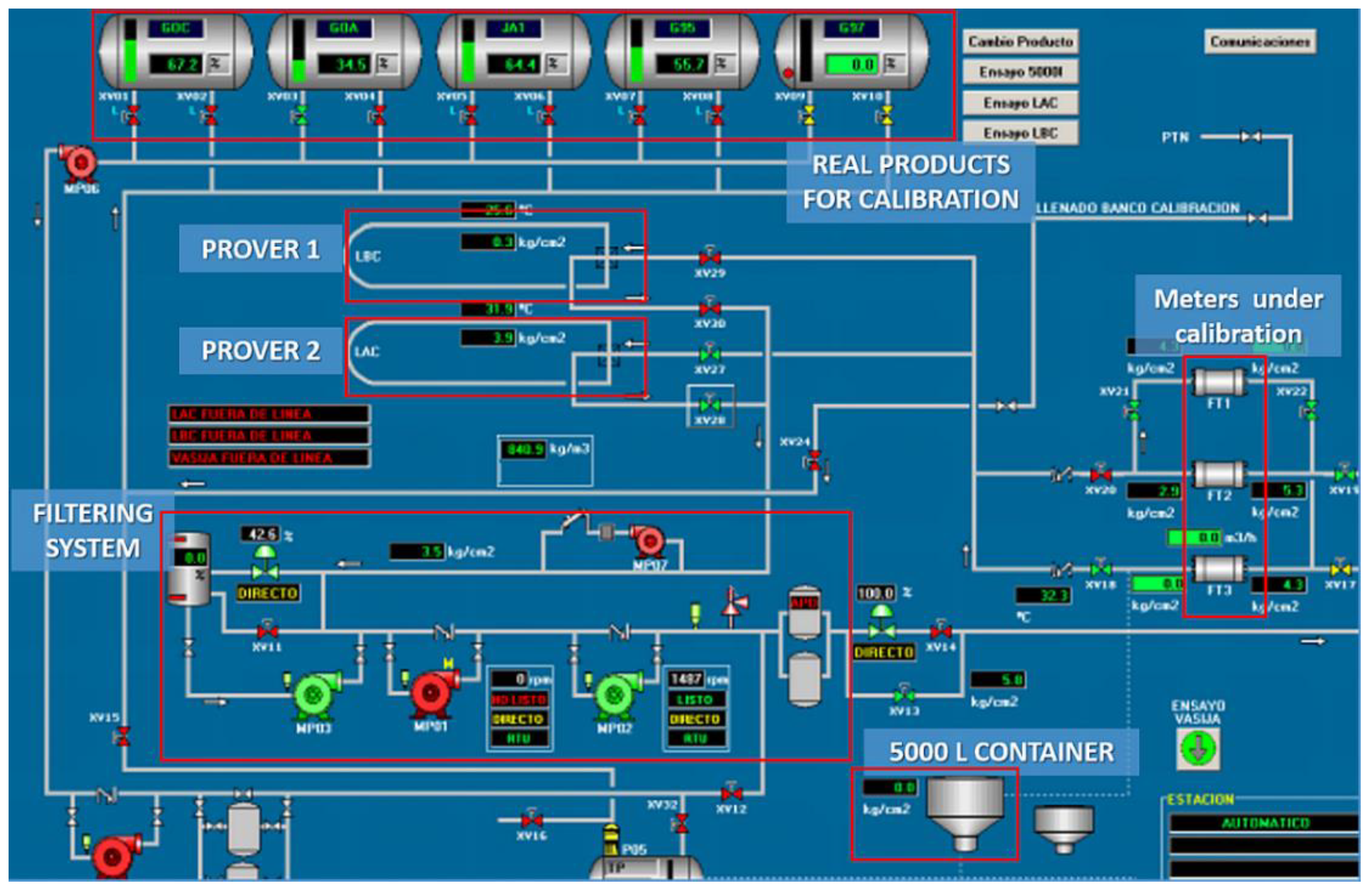
The schematic calibration set-up can be seen in Figure 1, as it appears in the control room of the calibration facility. This scheme includes all the components of the calibration facility and not only the ones used for this work. The calibration lab consists of two pipe provers (prover 1 and prover 2, seen in Figure 1) which receive the real products that are previously filtered by the filtering system (see real products for calibrations in Figure 1 and the filtering system in such figure). The location of the meters under calibration are also indicated (meters under calibration in the diagram). There is a dashed line that connects the 5000 L standard proving tank (at the bottom of Figure 1 and appearing as a 5000 L container) with the meter under calibration. So, the meters can be calibrated either by the tanks or by the provers.

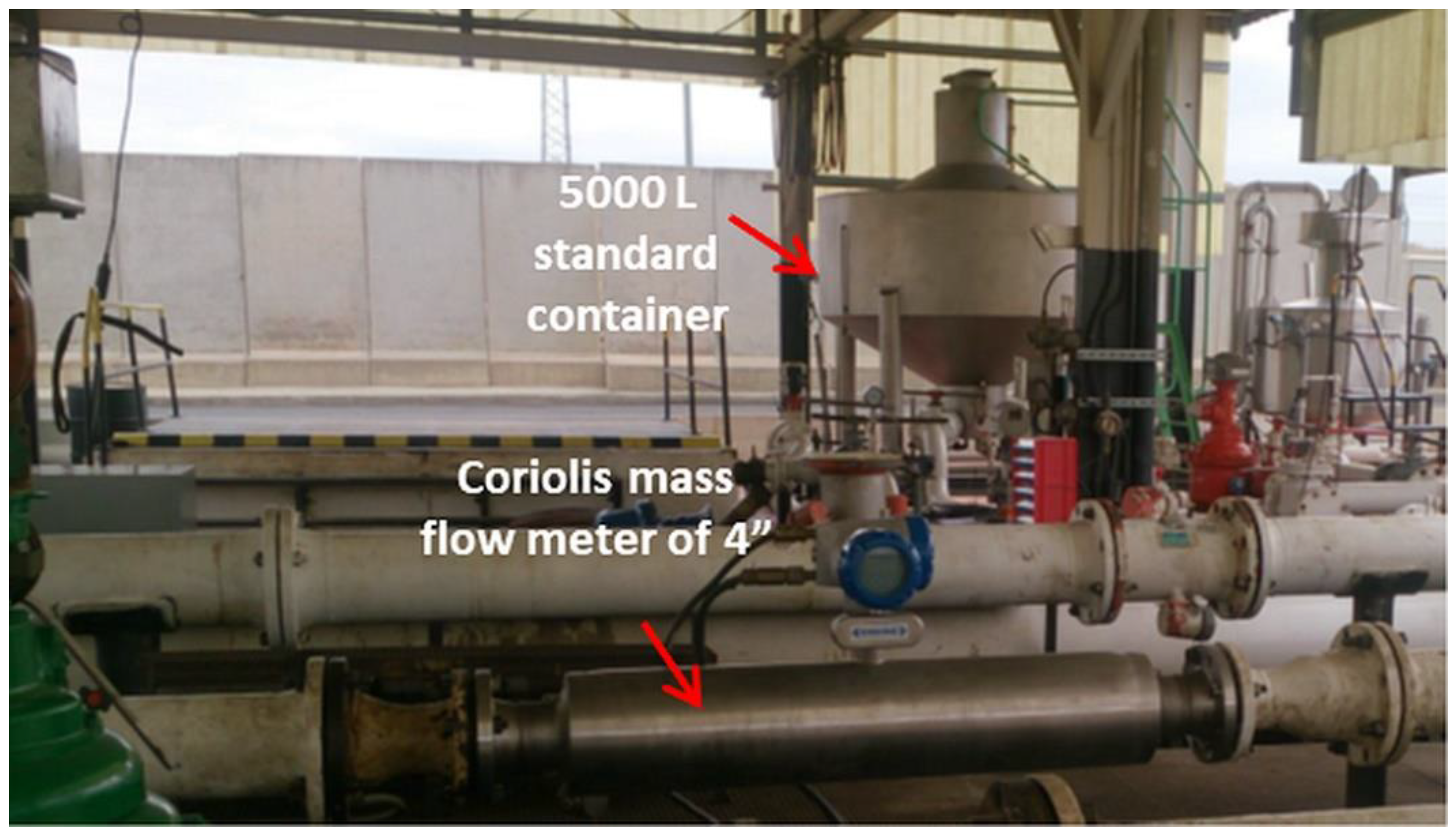
Figure 2 presents a photograph of the 5000-litre tank and a meter under calibration (in the figure, the meter is a Coriolis mass flow meter).

3. Adaptation of the Model Function for GUM-S1

According to GUM, there are two approaches to obtain the estimated value of the measurand Y: method 1 and method 2 [23]. Method 1 refers to obtaining y from:

y = f ({\bar{X}}_{1}, {\bar{X}}_{2}, ..., {\bar{X}}_{N})

(5)

where

{\bar{X}}_{1}, {\bar{X}}_{2}, ..., {\bar{X}}_{N}

are the arithmetic means of each input quantity and f is the model function.

Method 2 refers to obtaining the estimate y as:

\bar{Y} = (\sum_{k = 1}^{n} Y_{k}) / n

(6)

In general, if the model is not linear both methods are not compatible. If the repeatability range of the input quantities is low, both can be compatible.

The GUM-S1 method cannot implement method 2. If both methods are not compatible, only method 1 would be meaningful in the MCM (Monte Carlo method) framework as it requires a model function to obtain the measurand.

In case of lack of repeatability, both approaches are incompatible, the model cannot be linearized and GUM can not be used: GUM-S1 should be used with method 1.

In this work, it is shown how the application of GUM-S1 affects the measurand representation, considering the model function of the meter factor (MF) of a calibrated meter against a proving tank. When applying the GUM method, uncertainty calculation and measurand estimation can be independent, that is, method 1 can be used to estimate uncertainty and method 2 can be used to estimate the measurand. In fact, this is the situation in this case. However, if MCM is used, method 1 should be applied both for measurand and uncertainty estimation.

The MF calculation is performed in equation (2) by using method 2. So, in order to apply GUM-S1, equation (2) should be adapted [22]. The proposal of this work is substituting the type A evaluation of uncertainty of the measurand by a global additive contribution of a rectangular shape.

Therefore, the adapted model function of the calibration against a proving tank is as follows:

M F = \frac{V_{TAN K} \{1 + k_{v} [(t + δ t_{e}) - t_{REF}]\}}{V_{METER}} + δ M F_{REP}

(7)

where the quantities, t, V_METER and V_TANK are detailed in the following equations:

t = \bar{t} + δ t_{c a l} + δ t_{r e s} + δ t_{d r i f t} + δ t_{c o r r}

(8)

V_{T A N K} = {\bar{V}}_{T A N K} + δ V_{T A N K, c a l} + δ V_{T A N K, r e s} + δ V_{T A N K, d r i f t} + δ V_{T A N K, r a n g e}

(9)

V_{M E T E R} = {\bar{V}}_{M E T E R} + δ V_{M E T E R, r e s}

(10)

When applying the Monte Carlo method, the PDFs of the input quantities must be assigned as prior quantities based on the metrologist’s judgement [24]. The explanation of every input quantity as a random variable and its related probability density function PDF is detailed in Table 1.

4. General Methodology for Monte Carlo Simulation

In classical GUM method, two types of calculations are specified: the estimated value of the measurand and the typical uncertainty estimation, both calculations are separated and independent [1]. In GUM-S1, the simulation with random samples does not allow such separation [8].

According to [8], GUM-S1 provides a general approach to obtain an approximate numerical representation G of the distribution function G_Y for the measurand Y. The heart of the approach is repeated sampling from the PDFs for the input quantities Xi and the evaluation of the model in each case. The general description of the MCM approach would be as follows:

(a): Select the number M of Monte Carlo trails to be made.
(b): Generate M vectors, by sampling from the assigned PDFs, as realizations of the input quantities (X_i).
(c): For each such vector, form the corresponding model value of Y, yielding M model values.
(d): Sort these M models in strictly increasing order to provide G.
(e): Use G to form an estimate y of Y and the standard uncertainty u(y) associated with y.
(f): Use G to form an appropriate coverage interval for Y, for a stipulated coverage probability p, computing y_low and y_high being y_low is 2.5 th percentile (P2.5) and y_high 97.5 th percentile (P97.5), if a 95 % confidence level is desired.

When the PDF is not symmetrical, the uncertainty is not symmetrical either and the coverage factor is no longer meaningful. In fact, the coverage factor k is not considered in GUM-S1.

In GUM-S1 the expanded uncertainty is directly calculated with the approximate numerical representation of the PDF (G_Y) and there is no need to assume certain hypotheses on the normality or the effective degrees of freedom in a Student’s t-distribution.

If the MCM approach is used only for estimating the uncertainty, it must be proved that the measurand value y given by the MCM is compatible with the result given by the classical GUM method. When applying MCM the sample size M must be chosen. If the sample size is not large enough, different results could be obtained when repeating the simulation. According to GUM-S1, M could be in the order of 10⁶ but there is no guarantee that this or any specific pre-assigned number will suffice [8]. In this work, the adaptive Monte Carlo method (AMCM) was selected as this procedure controls the repeatability of the result and optimizes M, though its programming is more complicated. Nevertheless, in practice, a certain lack of repeatability is observed in the AMCM results, especially in the extreme percentiles of the PDF.

A basic implementation of an adaptive Monte Carlo procedure involves carrying out an increasing number of Monte Carlo trials until the various results of interest have stabilized in a statistical sense. AMCM is based on going from an M sample to a larger one of size h×M with a better statistical significance, being h a certain positive integer. The h value is obtained through an iterative process. Starting from the first sample of M size, more M-sized samples are generated independently at every iteration. The size samples which are being generated increase by 2× M, 3 × M, 4 × M, …, h × M until the statistical significance of h×M sample is optimal compared with the numerical tolerance of the measurand typical uncertainty

u (y)

The optimal sample is used to estimate the measurand value, its typical uncertainty, and consequently the expanded uncertainty. In the MCM framework, the numerical tolerance δ is the semi-width which delimits the last significant decimal of

u (y)

, and oscillates according to the number of significant figures selected to express

u (y)

. In this work, the number of significant figures is always two.

According to the GUM-S1 scheme, the value of M must be 10⁴ in order to reach a coverage probability less or equal to 99 %, which allows an equivalent Gaussian k=2 coverage probability (k=3 could not be reached). For a coverage larger than 99 %, M must be increased. The determination of h requires optimizing the statistics in every iteration. Therefore, the statistical descriptors

y

u (y)

y_{l o w}

y_{h i g h}

related to the h samples independently generated, are obtained. This results in a h-sized sample for every descriptor. The corresponding sample means would be

\bar{y}

\bar{u} (y)

{\bar{y}}_{l o w}

{\bar{y}}_{h i g h}

.The standard deviation from these are also calculated

s (\bar{y})

s [\bar{u} (y)]

s ({\bar{y}}_{l o w})

s ({\bar{y}}_{h i g h})

. In GUM-S1 the final h selected h^*, must be the first which complies with

2 s (\bar{y})

2 s [\bar{u} (y)]

2 s ({\bar{y}}_{l o w})

2 s ({\bar{y}}_{h i g h})

being less than the numerical tolerance δ.

5. Proposals for AMCM Improvement

The selection criteria for the h value in GUM-S1 assumes that the mean values of the statistical descriptors

y

u (y)

y_{l o w}

y_{h i g h}

at every iteration follow a normal distribution and, therefore, such selection criterion would have a 95.45 % confidence level. Strictly speaking, this is correct when h is large enough, but in practice, this is not so. This implies that the factor multiplying

s (\bar{y})

s [\bar{u} (y)]

s ({\bar{y}}_{l o w})

s ({\bar{y}}_{h i g h})

is underestimated.

In this work, the first proposal is to use a coverage factor from a Student’s t-distribution with h–1 degrees of freedom. In the case that the number of degrees of freedom is large enough and compatible with Gaussian statistics, the Student’s t-distribution itself will be very similar to a Gaussian and the GUM-S1 criteria could be used. In principle, the Student’s t-distribution coverage factor which should be used would be the one corresponding to a 95.45 % confidence level, as in GUM-S1 the standard deviations

s (\bar{y})

s [\bar{u} (y)]

s ({\bar{y}}_{l o w})

s ({\bar{y}}_{h i g h})

are multiplied by 2. A higher confidence level could be used (for instance 99.73 %) but this would imply more iterations to converge h.

Therefore, the first improvement proposal for AMCM consists of changing the acceptance and rejection criterion for h from GUM-S1 so that this criterion is also adaptive; that is, the stricter the criterion the lower the h value. The level of confidence in the optimization of h would be 95.45 % (GUM-S1) or higher depending on the requirements in each case.

As a second improvement, this work proposes the validation of the AMCM repeatability by using δ as a reference. In practice, when a new cycle of iterations is performed, the lack of repeatability could lead to the variability of

y

u (y)

y_{l o w}

y_{h i g h}

and a new value of h,

h \neq h'

would be obtained. Therefore, the proposal considers R repetitions of the adaptive cycle and checks if

y

u (y)

y_{l o w}

y_{h i g h}

are changing if rounded according to δ. This rounding process is done first in

u (y)

according to δ and then in

y

y_{l o w}

y_{h i g h}

according to

u (y)

The precision of the final results of AMCM must be always adjusted to δ; otherwise, a spurious variability would always be observed. In order to come up with a stable result, the R values for

y

u (y)

y_{l o w}

y_{h i g h}

will be averaged and rounded according to δ. The stability will be confirmed by calculating the standard deviations of the sample means multiplied by 2 or 3, depending on the requirements, and the results will be checked to be zero after rounded according to δ. This will ensure that the repeatability of the results

y

u (y)

y_{l o w}

y_{h i g h}

will have a 95.45 % or 99.73 % confidence level whenever R is large enough. In this work, R is taken as 50.

In the third place, the diagnosis of the empirical PDF of the measurand is proposed. For that purpose, the estimation of skewness and kurtosis are combined with normality contrasts. An index of deviation from normality based on the kurtosis is proposed to quantify the diagnostics. It must be checked that the skewness is zero to validate the symmetry of the interval [

y_{l o w}

y_{h i g h}

] in respect to y, before calculating the expanded uncertainty and the k factor. Three hypothesis tests are proposed: distribution function tests (Lilliefors and Anderson-Darling test), momentum tests (D’Agostino and Omnibus de D’Agostino tests for skewness and kurtosis), and squared minimum correlation (Shapiro Wilk). With these tests, the samples are checked to be normal with a 95 % confidence level. If there is no rejection, normality cannot be assured.

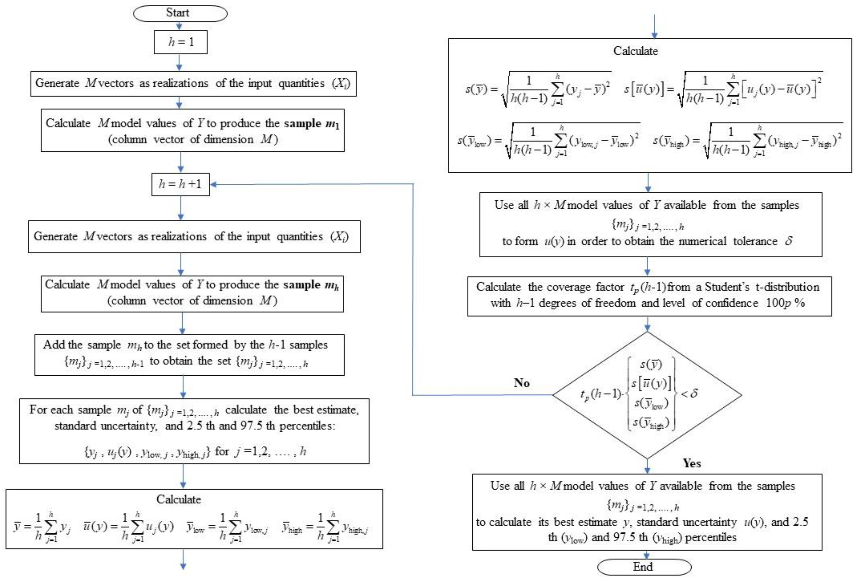
In Figure 3 there is a flow chart representing all the steps of the proposed methodology.

6. Results and Discussion

The case presented is the calibration of a flow meter against a standard tank to obtain the meter factor (MF). The results are gathered in two tables; Table 2 shows the results for the meter factor, its standard uncertainty and its lower and upper limits for AMCM and GUF and Table 3 shows the results for the expanded uncertainty, the coverage factor, the relative expanded uncertainty (W), and the numerical tolerance δ for both methods.

As can be seen, AMCM U(MF) is lower than GUF. This means a 7,1 % decrease in relative expanded uncertainty W(MF). MF from AMCM is identical to MF from GUF: which implies that the model function is linear within the range of the input quantities.

The GUF value for u(MF) with two significant figures is identical to the value for AMCM: the law of propagation of uncertainty of the GUM method could be applied in this case to estimate the standard uncertainty.

The AMCM value for de U(MF) is 6 % lower than the GUF value due to the different coverage factors of both methods, so the MF distribution is not Gaussian.

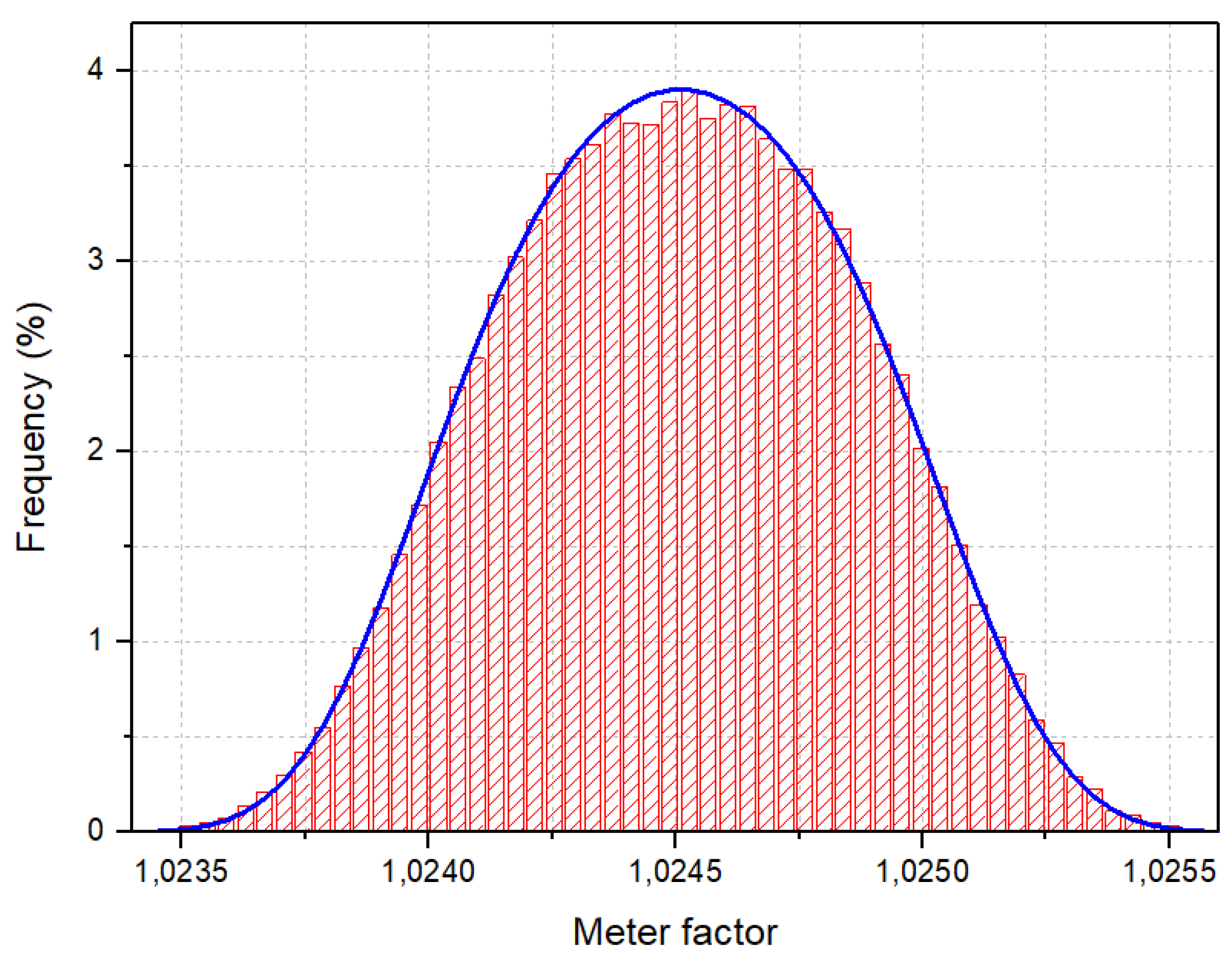
The tests applied reject the normality, and the kurtosis values (-0.55) are lower than in a normal distribution.

The normality deviation index shows a deviation of –18.3 % in respect to a Gaussian.

The classical GUM method would never result in the correct PDF as the Student’s t-distribution has a positive excess kurtosis.

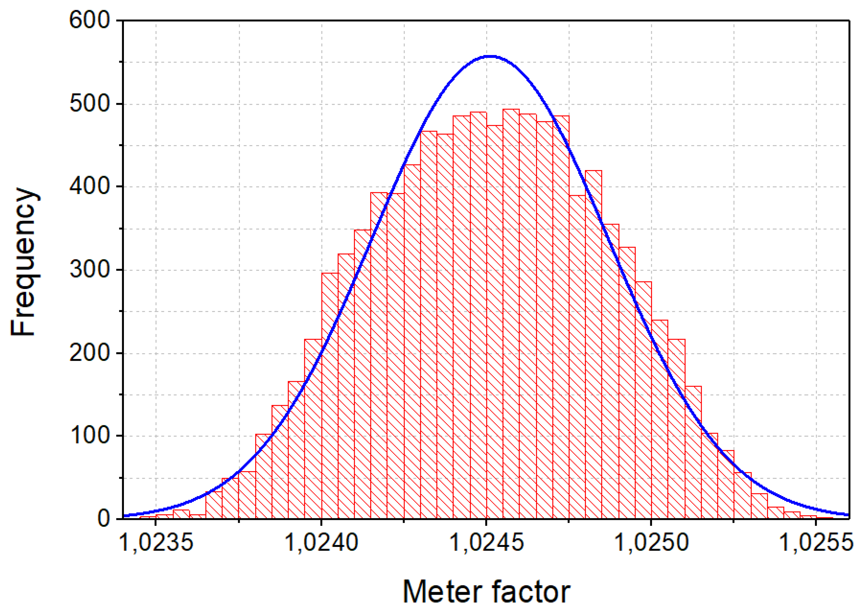
In Figure 4, the MF histogram as obtained from the AMCM is fitted to a normal distribution. As can be observed, the resulting distribution is clearly deviated from the Gaussian with a negative excess kurtosis.

Though the MF model function can be linearized, the deviation from normality indicates that the conditions for the Central Limit Theorem are not fulfilled.

According to GUM-S1 in NOTE 4 of the 5.7.2 subsection, the lack of normality is due to the fact that the rectangular distribution assigned to the MF repeatability is dominant. This can be proved by simulating the PDF and removing the repeatability contribution. The function model result of the sum of a Gaussian and a dominant rectangular distribution is a Flatten-Gaussian PDF [20] as it is the one proposed for the MF.

A specific simulation (non-adaptive) of 10⁵ samples has been carried out to fit the empirical distribution to a Flatten-Gaussian PDF whose equation is [20]:

g_{MF} (ξ) = A \exp [- a {(ξ - c)}^{2} - b {(ξ - c)}^{4}]

(11)

where A is a normalization constant, a and b are parameters dependent on the distribution momenta and, c, is the best estimate of the MF. The fitting plot is shown in Figure 5 and the estimated parameters are presented in Table 4. The goodness of fit is given by the adjusted R- Squared whose value is 0.99914.

Finally, it has been checked that the estimated A is compatible with the A value (0.03868) calculated from a and b with the expression given in [20].

Some authors also detect a non-gaussian dominant component but they do not identify it as such [13]. Other authors interpret the presence of a rectangular dominant component as a consequence of the lack of a linearity measurement model [9] but in fact, the model was linear. The use of this PDF guarantees the uncertainty requirement to be transferable to other users. In fact, only if the PDF is known, further Monte Carlo simulations can be performed.

7. Conclusions

In this work, the expanded uncertainty of the ratio between measured volume and reference volume called Meter Factor (MF) for the calibration of a flow meter against a proving tank is estimated by using the Adaptive Monte Carlo Method. In this way, the shortcomings of the traditional GUM method are avoided and the following innovations for the AMCM are proposed:

The convergence regulation of the AMCM by applying the coverage factors of a Student’s t-distribution.

The repeatability validation of the AMCM through the realization of 50 iterations of the adaptive cycle to assure the numerical stability of the results.

The analysis of the measurand PDF by estimating its skewness, kurtosis, and testing its normality.

For the flow meters used in the custody transfer and calibrated against a standard proving tank, the proposed methodology reduces the uncertainty compared to the one calculated through GUM.

In fact, for the case study, it was proved that GUM did not result in the correct PDF qualitatively for the MF as it is neither Gaussian nor Student’s t-distribution. The analytical expression proposed for the PDF of the MF is a Flatten-Gaussian.

Author Contributions

“Conceptualization, A García-Berrocal and P.Carmona; methodology, A García-Berrocal.; software, A García-Berrocal, C. Montalvo ; validation, A García-Berrocal, C. Montalvo and P.Carmona.; formal analysis, A García-Berrocal, C. Montalvo and R.García-Álvarez; investigation, A García-Berrocal, C. Montalvo.; resources, P.Carmona.; A García-Berrocal, C. Montalvo, X.; writing—original draft preparation, A García-Berrocal and C. Montalvo; writing—review and editing, A García-Berrocal, C. Montalvo, P.Carmona and R.García-Álvarez.; visualization, C. Montalvo and R.García-Álvarez.; supervision, P.Carmona ; project administration, A García-Berrocal.; funding acquisition, A García-Berrocal. All authors have read and agreed to the published version of the manuscript.”

Funding

This work has been funded by the EXOLUM-UPM Chair in Metrology at the Universidad Politécnica de Madrid. This program develops the scientific collaboration between UPM (Spain) and EXOLUM Corporation, with the purpose of promoting knowledge of metrology. EXOLUM is the leading company in Spain for oil product transportation and storage and is one of the largest private companies in its sector at an international level. In addition, the authors wish to thank the Metrology Laboratory of EXOLUM in Loeches (Madrid) for providing the data analysed in this work.

Data Availability Statement

Data not available due to commercial and confidentiality restrictions.

Acknowledgments

The authors would like to thank Carlos García-Berrocal for careful review of the language of the manuscript.

Conflicts of Interest

The authors declare no conflicts of interest.

1	Monte Carlo Method (MCM)

References

Joint Committee for Guides in Metrology (JCGM) et al., “Evaluation of measurement data — An introduction to the ‘Guide to the expression of uncertainty in measurement’ and related documents,” International Organization for Standardization Geneva ISBN, vol. 3, no. October, 2008.
H. F. F. Castro, “Validation of the GUM using the Monte Carlo method when applied in the calculation of the measurement uncertainty of a compact prover calibration,” Flow Measurement and Instrumentation, vol. 77, p. 101877, Mar. 2021. [CrossRef]
H. F. F. Castro, “Mathematical modeling applied to the uncertainty analysis of a tank prover calibration: Understanding the influence of calibration conditions on the GUM validation using the Monte Carlo method,” Flow Measurement and Instrumentation, vol. 96, p. 102547, Apr. 2024. [CrossRef]
García-Berrocal, C. Montalvo, P. Carmona, and J. Blázquez, “The Coriolis mass flow meter as a volume meter for the custody transfer in liquid hydrocarbons logistics,” ISA Trans, vol. 90, pp. 311–318, Jul. 2019. [CrossRef]
Barateiro, A. Faria, J. Farias Filho, K. Maggessi, and C. Makarovsky, “Fiscal Measurement and Oil and Gas Production Market: Increasing Reliability Using Blockchain Technology,” Applied Sciences 2022, Vol. 12, Page 7874, vol. 12, no. 15, p. 7874, Aug. 2022. [CrossRef]
E. Savio, L. De Chiffre, S. Carmignato, and J. Meinertz, “Economic benefits of metrology in manufacturing,” CIRP Annals, vol. 65, no. 1, pp. 495–498, 2016. [CrossRef]
R. Kacker, K.-D. Sommer, and R. Kessel, “Evolution of modern approaches to express uncertainty in measurement,” Metrologia, vol. 44, no. 6, pp. 513–529, Dec. 2007. [CrossRef]
“JCGM 101: Evaluation of Measurement Data - Supplement 1 to the ‘Guide to the Expression of Uncertainty in Measurement’ - Propagation of Distributions Using a Monte Carlo Method.” Accessed: May 28, 2024. [Online]. Available: https://www.sci.utah.edu/~kpotter/Library/Papers/jcgm:2008:PDMC/index.html.
H. Alkhatib, I. Neumann, and H. Kutterer, “Uncertainty modeling of random and systematic errors by means of Monte Carlo and fuzzy techniques,” Journal of Applied Geodesy, vol. 3, no. 2, Jan. 2009. [CrossRef]
Chen and C. Chen, “Comparison of GUM and Monte Carlo methods for evaluating measurement uncertainty of perspiration measurement systems,” Measurement, vol. 87, pp. 27–37, Jun. 2016. [CrossRef]
M. Forster, F. Seibold, T. Krille, C. Waidmann, B. Weigand, and R. Poser, “A Monte Carlo approach to evaluate the local measurement uncertainty in transient heat transfer experiments using liquid crystal thermography,” Measurement, vol. 190, p. 110648, Feb. 2022. [CrossRef]
G. M. Mahmoud and R. S. Hegazy, “Comparison of GUM and Monte Carlo methods for the uncertainty estimation in hardness measurements,” International Journal of Metrology and Quality Engineering, vol. 8, p. 14, 2017. [CrossRef]
Runje, A. Horvatic, V. Alar, S. Medic, and A. Bosnjakovic, “Examples of measurement uncertainty evaluations in accordance with the revised GUM,” J Phys Conf Ser, vol. 772, p. 012008, Nov. 2016. [CrossRef]
R. Willink, “Difficulties arising from the representation of the measurand by a probability distribution,” Meas Sci Technol, vol. 21, no. 1, p. 015110, Nov. 2009. [CrossRef]
M. G. Cox and B. R. L. Siebert, “The use of a Monte Carlo method for evaluating uncertainty and expanded uncertainty,” Metrologia, vol. 43, no. 4, p. S178, Aug. 2006. [CrossRef]
Y. Li, Z. Wang, Y. Tang, and Z. Shang, “Application of adaptive Monte Carlo method to evaluate pose uncertainty in monocular vision system,” https://doi.org/10.1117/1.OE.61.6.061413, vol. 61, no. 6, p. 061413, Mar. 2022. [CrossRef]
J. Singh, N. Bura, K. Kaushik, L. A. Kumaraswamidhas, and N. Dilawar Sharma, “Investigation of contribution of number of trials in Monte Carlo simulation for uncertainty estimation for a pressure balance,” Transactions of the Institute of Measurement and Control, vol. 43, no. 16, pp. 3615–3624, Dec. 2021. [CrossRef]
X. L. Wen, Y. B. Zhao, D. X. Wang, and J. Pan, “Adaptive Monte Carlo and GUM methods for the evaluation of measurement uncertainty of cylindricity error,” Precis Eng, vol. 37, no. 4, pp. 856–864, Oct. 2013. [CrossRef]
G. Wübbeler, P. M. Harris, M. G. Cox, and C. Elster, “A two-stage procedure for determining the number of trials in the application of a Monte Carlo method for uncertainty evaluation,” Metrologia, vol. 47, no. 3, pp. 317–324, Jun. 2010. [CrossRef]
J. Blázquez, A. García-Berrocal, C. Montalvo, and M. Balbás, “The coverage factor in a Flatten–Gaussian distribution,” Metrologia, vol. 45, no. 5, p. 503, Aug. 2008. [CrossRef]
P. Fotowicz, “Modified Monte Carlo Method for Calculating the Expanded Measurement Uncertainty,” Advances in Intelligent Systems and Computing, vol. 352, pp. 67–74, 2015. [CrossRef]
“API MPMS 4.9.3 - Manual of Petroleum Measurement Standards Chapter 4-Proving Systems Section 9-Methods of Calibration for Displacement and Volumetric Tank Provers Part 3—Determination of the Volume of Displacement Provers by the Master Meter Method of Calibration Measurement Coordination | GlobalSpec.” Accessed: May 28, 2024. [Online]. Available: https://standards.globalspec.com/std/9958017/API%20MPMS%204.9.3.
W. Bich, L. Callegaro, and F. Pennecchi, “Non-linear models and best estimates in the GUM,” Metrologia, vol. 43, no. 4, 2006. [CrossRef]
J. Singh, L. A. Kumaraswamidhas, N. Bura, and N. Dilawar Sharma, “A Monte Carlo simulation investigation on the effect of the probability distribution of input quantities on the effective area of a pressure balance and its uncertainty,” Measurement, vol. 172, p. 108853, Feb. 2021. [CrossRef]

Figure 1. Calibration set-up scheme.

Figure 2. Photograph of the tank and a flow meter under calibration in the facility.

Figure 3. Flow chart of the proposed methodology.

Figure 4. In red, a histogram of the empirical PDF of the MF. In blue, normal fit.

Figure 5. Flatten-Gaussian fit of the MF empirical distribution.

Table 1. Explanation of input quantities in the model function.

Input quantity	Contribution to the MF model function	PDF
$δ M F_{REP}$	Repeatability of the MF	Rectangular
$δ t_{e}$	Temperature gradient inside the tank	Rectangular
$\bar{t}$	Average measured temperature in the tank	Constant
$δ t_{c a l}$	Calibration of temperature sensor in the tank	Gauss
$δ t_{r e s}$	Resolution of temperature sensor in the tank	Rectangular
$δ t_{d r i f t}$	Drift of temperature sensor in the tank	Rectangular
$δ t_{c o r r}$	Correction of temperature sensor in the tank	Rectangular
${\bar{V}}_{T A N K}$	Average measured volume in the tank	Constant
$δ V_{T A N K, c a l}$	Calibration of tank volume	Gauss
$δ V_{T A N K, r e s}$	Resolution of tank volume	Rectangular
$δ V_{T A N K, d r i f t}$	Drift of tank volume	Rectangular
$δ V_{T A N K, r a n g e}$	Range of tank volume	Rectangular
${\bar{V}}_{M E T E R}$	Average measured meter volume	Constant
$δ V_{M E T E R, r e s}$	Resolution of meter	Rectangular

Table 2. Meter factor and standard meter factor uncertainty for both methods: AMCM and GUF.

AMCM			GUF
MF	1.024 51	dimensionless	MF	1.024 51	dimensionless
u(MF)	0.000 36	dimensionless	u(MF)	0.000 356 5	dimensionless
MF_low	1.023 84	dimensionless	MF_low	N/A	-
MF_high	1.025 18	dimensionless	MF_high	N/A	-

Table 3. Meter factor expanded uncertainty, coverage factor, W and numerical tolerance δ for both methods: AMCM and GUF.

AMCM			GUF
U(MF)	0.000 67	dimensionless	U(MF)	0.000 713	dimensionless
k	1.86	dimensionless	k	2	dimensionless
W(MF)	0.065	%	W(MF)	0.070	%
δ	0.000 005	dimensionless	δ	N/A	-

Table 4. Estimated parameters from the Flatten-Gaussian fit.

Estimated parameter	Standard error
A = 0.038 60	0.000 15
a = 1.766×10⁶	0.062×10⁶
b = 3,616×10¹²	0.162×10¹²

Disclaimer/Publisher’s Note: The statements, opinions and data contained in all publications are solely those of the individual author(s) and contributor(s) and not of MDPI and/or the editor(s). MDPI and/or the editor(s) disclaim responsibility for any injury to people or property resulting from any ideas, methods, instructions or products referred to in the content.

© 2024 by the authors. Licensee MDPI, Basel, Switzerland. This article is an open access article distributed under the terms and conditions of the Creative Commons Attribution (CC BY) license (http://creativecommons.org/licenses/by/4.0/).

Copyright: This open access article is published under a Creative Commons CC BY 4.0 license, which permit the free download, distribution, and reuse, provided that the author and preprint are cited in any reuse.

MDPI Initiatives

Important Links

Choose an area of interest and we will send you notifications of new preprints at your preferred frequency.

Disclaimer