1. Introduction
Landslides, particularly those triggered by rainfall, pose a significant threat to human life and infrastructure worldwide. The global incidence of landslides is alarming, with thousands of events reported each year [
1], often resulting in catastrophic damage and loss of life. Japan, with its mountainous terrain and frequent typhoons, faces a recurring threat of landslides caused by rainfall. Saito [
2] reports numerous such events each year, worsened by intense seasonal rains and typhoons. These landslides cause destruction to infrastructures and significant economic losses and disruptions [
3]. Therefore, it is crucial to have effective monitoring and early warning systems in place in these regions. Understanding the factors that contribute to slope failures, such as rainfall patterns and soil saturation levels, is essential for the development of such systems. Research indicates that accurate prediction and timely alerts can mitigate the impact of these disasters [
4,
5]. Consequently, there is a growing focus on enhancing the tools and techniques utilized for monitoring slopes at risk of landslides.
To comprehend the mechanisms of slope failure, many researchers have conducted small-scale slope model experiments within laboratory settings [
6,
7,
8,
9,
10]. These experiments aim to replicate real-world conditions to study the behavior of slopes under various scenarios. Common equipment used in these studies includes inclinometers, which measure the angle of slope movements, and pore pressure transducers, which monitor water pressure within the soil. Additionally, soil moisture sensors are crucial for detecting changes in soil water content, a key factor in slope stability [
11,
12,
13,
14]. These sophisticated instruments provide detailed insights into the processes leading to slope failure, contributing significantly to our understanding of landslide dynamics. However, the high cost and complexity of these instruments limit their widespread application, especially in resource-constrained settings. Therefore, there is a need for more accessible and cost-effective monitoring solutions. Although some progress has been made in this area [
14,
15,
16,
17], many existing systems remain impractical for widespread application due to challenges related to affordability, scalability, need for expertise, and maintenance in remote or developing regions. These limitations underscore the ongoing inadequacies in landslide monitoring systems, particularly in susceptible locations that would benefit from more long-term solution.
With the current advancements in technology, the development of low-cost sensors integrated with the Internet of Things (IoT) presents a promising solution. IoT technology enables the remote collection and transmission of data, making it possible to monitor slope failure vulnerability in multiple sites simultaneously and in real-time [
18,
19,
20]. One notable example is the SKU:SEN0193, a low-cost capacitive moisture sensor that offers a feasible alternative for widespread monitoring and has been widely studied for agricultural purposes [
21,
22,
23,
24]. This sensor is not only affordable but also capable of providing real-time data. In the context of landslide monitoring and mitigation, SKU:SEN0193 has the potential to be used effectively in landslide early warning systems. Moreover, integrating this soil moisture sensor with IoT platforms allows for continuous monitoring and data analysis, enhancing the effectiveness of landslide prediction models. This approach not only reduces costs but also improves the accessibility of landslide monitoring technologies.
To ensure the accuracy and reliability of this low-cost moisture sensor, calibration on specific soil types and properties is essential, as the calibration results significantly influence sensor readings, making calibration a critical step [
22,
24,
25]. This research aims to evaluate the performance of low-cost capacitive moisture sensors (SKU:SEN0193) by developing calibration equations to predict soil moisture content. To verify the results, the moisture sensors were tested in slope model experiments under laboratory condition in different rainfall intensities. After the completion of the slope model experiment, the moisture contents detected by the sensors were compared against the actual soil moisture contents. The validation of calibration equations through slope model experiments shows the effectiveness of the moisture sensors in delivering accurate data, thus supporting cost-effective solutions for a landslide early warning system.
2. Materials and Methods
2.1. Data Acquisition
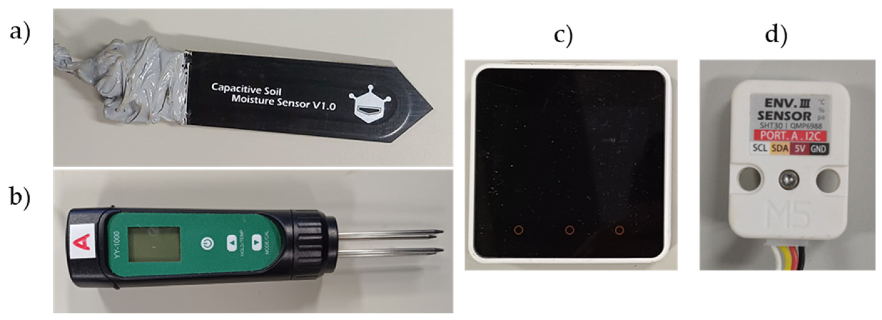
Six low-cost capacitive soil moisture sensors SKU:SEN0193 from DFRobot were used in this study. Each sensor operates within a voltage input range of 3.3 to 5.5 V, measures 9.8 × 2.3 cm (L × W) and weights15 grams, making it compatible with low-power microcontrollers [
26]. Its surface is coated with a corrosion-resistant material, enhancing its durability. To protect the electronic components of the moisture sensors from short circuits, oxidation, and physical damage during experiments, the electronic parts were covered with silicone, making them waterproof. From the following, the term moisture sensor is used, instead of SKU:SEN0193. In addition, two Slyfox soil moisture meters were used to measure the soil temperature. This commercial device, designed specifically for agricultural applications, incorporates a temperature measurement feature for soil assessment [
27]. Lastly, an ENV III environmental sensor from M5Stack was employed to measure room temperature, humidity, and atmospheric pressure. The ENV III sensor is capable of measuring temperatures ranging from -40 to 125 °C, relative humidity from 0 to 100 %, and air pressure from 300 to 1100 hPa. The equipment used for this study is shown in
Figure 1.
The moisture sensor and ENV III were connected to the M5Stack Core2, serving as a microcontroller unit for aggregating and transmitting data to a cloud server via the internet. The M5Stack Core2 has dimensions of 5.4 × 5.4 × 1.6 cm (L × W × H) and is equipped with a 390mAh 3.7V built-in battery. It features a dual-core Xtensa
® 32-bit 240MHz processor, onboard 16MB Flash and 8MB PSRAM, and a USB Type-C interface for charging, program downloading, and serial communication. The M5Stack Core2 was programmed using the Arduino programming language. To monitor and download data from the cloud server, an open-source Internet of Things (IoT) data visualization tool Ambient (
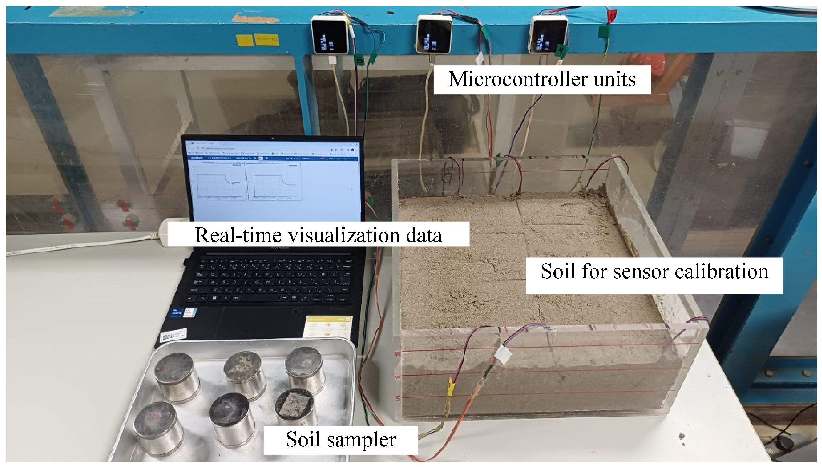
https://ambidata.io/) was utilized. The experiment setup is presented in (
Figure 2), while the component and total cost for the study was around US
$ 260 (
Table 1).
2.2. Soil Properties and Calibration Process
Commercially available silica sand grade 7 was used for this research, hereafter referred to as K7 sand. This sand was chosen because it is frequently utilized in slope model experiments to examine the failure mechanisms associated with rainfall-induced landslides, particularly in scenarios where sandy soils play a critical role in the triggering process [
28,
29,
30,
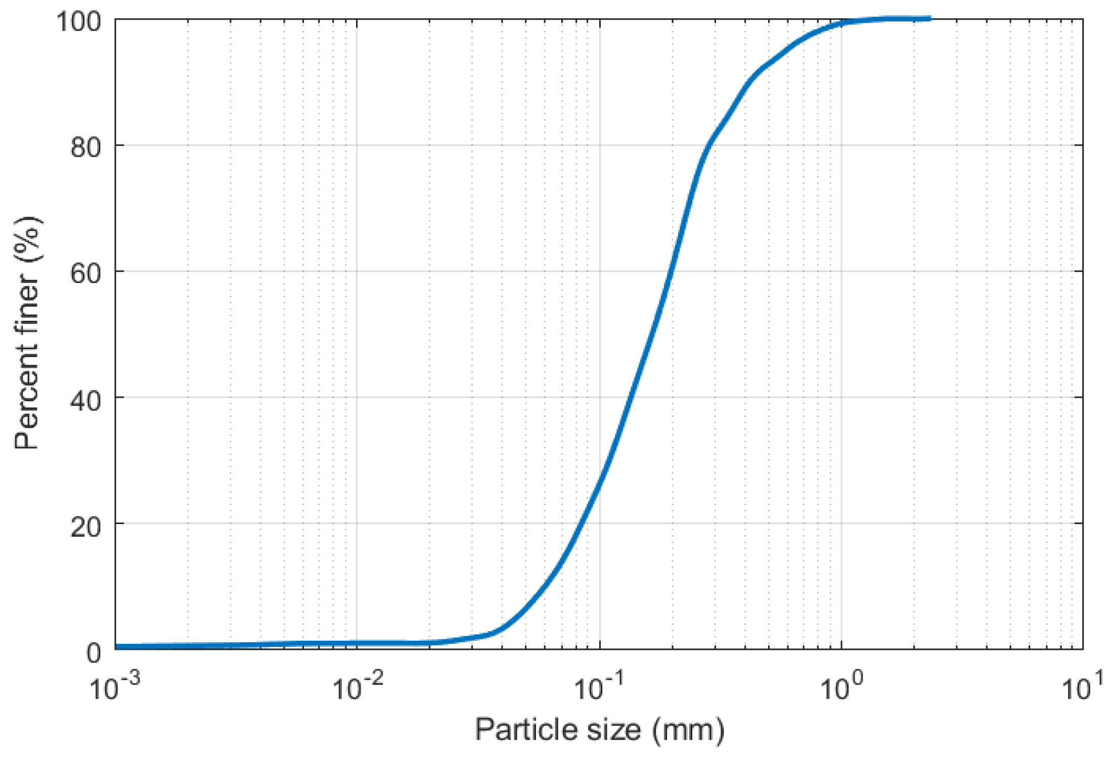
31]. The soil particle size distribution and properties are presented in
Figure 3 and
Table 2.
To achieve precise calibration and ensure the accuracy of the moisture sensor, a calibration experiment was carefully designed. Upon completion, the output was the calibration equation for each soil moisture sensor. To verify these calibration equations, three slope model experiments with different rainfall intensities were conducted. In the slope model experiments, the raw data from the soil moisture sensors were converted using the calibration equation to measure the soil moisture content. Therefore, the calibration process was designed according to the slope model experiment, since the sensor measurements during calibration are strongly influenced by sample preparation and calibration protocols [
32,
33]. The calibration experiment involves ten steps:
The dimensions of the soil box were measured, and the required amount of soil was determined. Additionally, the weight of soil for two layers was calculated. The soil box was then marked at heights of 5 cm and 10 cm for the first and second layers, respectively.
Water equivalent to 5% of the weight of the soil was mixed to the oven-dried soil.
Half of the soil prepared in step 2 was placed in the soil box to create the first layer, after which it was compacted to match the height of the first layer.
Six moisture sensors were placed on top of the first soil layer. The moisture sensors were positioned at an adequate distance from one another to prevent any potential interference.
The remaining soil-water mixture prepared in Step 2 was placed and compacted to match the height of the second layer.
The soil box was covered with a plastic sheet to minimize potential moisture evaporation and the soil sample was left to homogenized for 20 to 40 minutes.
The moisture sensors recorded three measurements (5 minutes each). The average value of these measurements was used for the analysis of moisture sensor calibration.
Both soil and room temperatures were recorded.
Soil samples were collected from locations near the moisture sensors, and the actual soil moisture content was measured.
Steps 2 through 9 were repeated, increasing the water incrementally by 5% until the soil sample indicates saturation conditions.
To fit and evaluate both linear and non-linear regression models, the programming language and numeric computing environment MATLAB version R2023b was utilized. The first model was linear, the second was logarithmic and the quadratic was considered as polynomial in the third model. The best-fitted model was determined based on its high coefficient of determination (R2) and low root mean square error (RMSE).
2.3. Slope Model Experiment
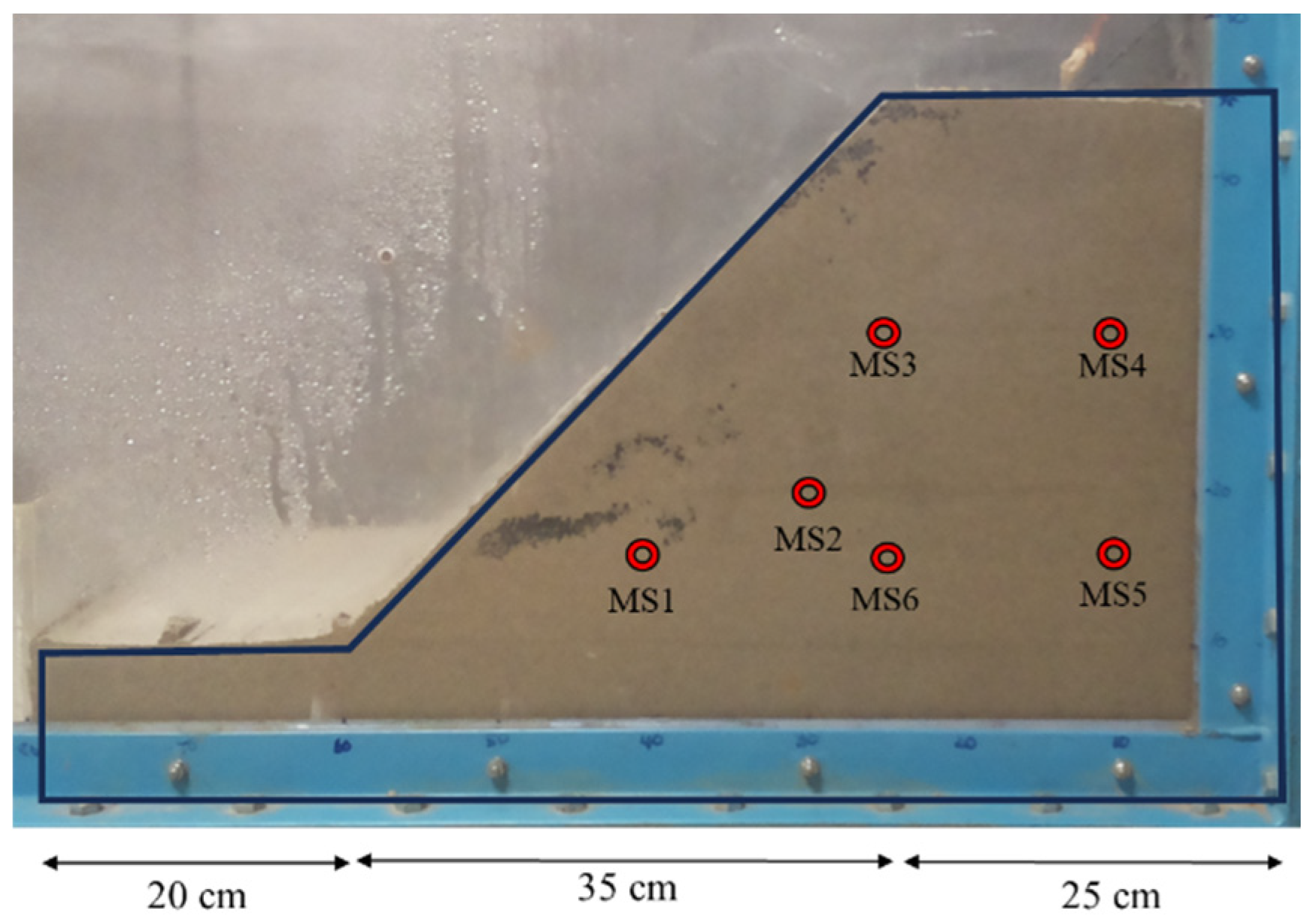
Slope model experiment was designed to test the soil moisture sensors in a controlled environment under rainfall intensities of 100, 70, and 45 mm/h. The dimensions of the slope model and the positions of the sensors for the experiments are illustrated in
Figure 4. The slope model measured 80 cm in length, 40 cm in width, and 45 cm in height. The slope angle was set to 45°. This slope angle was chosen as it represents a practical compromise between stability and the risk of failure, allowing for effective modeling of real-world conditions. The slope model was constructed by compacting the soil every 5 cm, while the base layer was compacted at 10 cm of height. There were a total of eight soil layers with a soil dry density of 1.40 g/cm
3 and an initial water content of 10%. A rainfall simulator was designed to simulate uniform and continuous rainfall with different rainfall intensities. The rainfall is generated by nozzles attached to the rainfall simulator frame installed above the flume tank.
After each experiment, soil samples were collected from the near respective moisture sensors. The purpose is to measure the actual moisture contents (
) of the soil and verify the result with the moisture contents monitored by the sensors. Moisture content from the collected soil samples were measured by oven-drying them. It is expressed by the weight ratio difference between wet and dry samples. The water mass ratio is established by drying the soil samples in an oven at a temperature of 100–110 °C until a constant mass is reached, followed by measuring the weight of the soil samples before and after the drying process. The calculation is following the formula:
where
is mass of the sample and container,
mass of the oven-dried sample and container,
is mass of container in gram.
2.4. Statistical Evaluation
Three statistical indicators were used to quantify the accuracy of the calibration equations: coefficient of determination (R
2), root mean square error (RMSE), and mean biased error (MBE) [
24,
34]. R
2 describes the correlation between the calibrated and actual values (Eq. 2), RMSE was used to describe the accuracy between calibrated and actual values (Eq. 3), and mean biased error (MBE) was used to measure the deviation of overall calibration results (Eq. 4).
where
is the sample size,
is the sensor measured value,
is the mean sensor measured value,
is the actual value, and
is the mean actual value.
3. Results
3.1. Moisture Sensor Calibration
The SKU:SEN0193 is one of the moisture sensors designed for integration into the Internet of Things (IoT), allowing for operation at low power levels ranging from 3.3 to 5V. Verifying the operating voltage of 3.3 to 5V in the moisture sensor, including checking the timer chips and voltage regulator [
35,
36] was the initial step before utilizing it. In this study, the authors were using SKU:SEN0193 v1.0. Both the timer chip and voltage regulator for all moisture sensors were examined and found to operate within the 3.3 to 5V range.
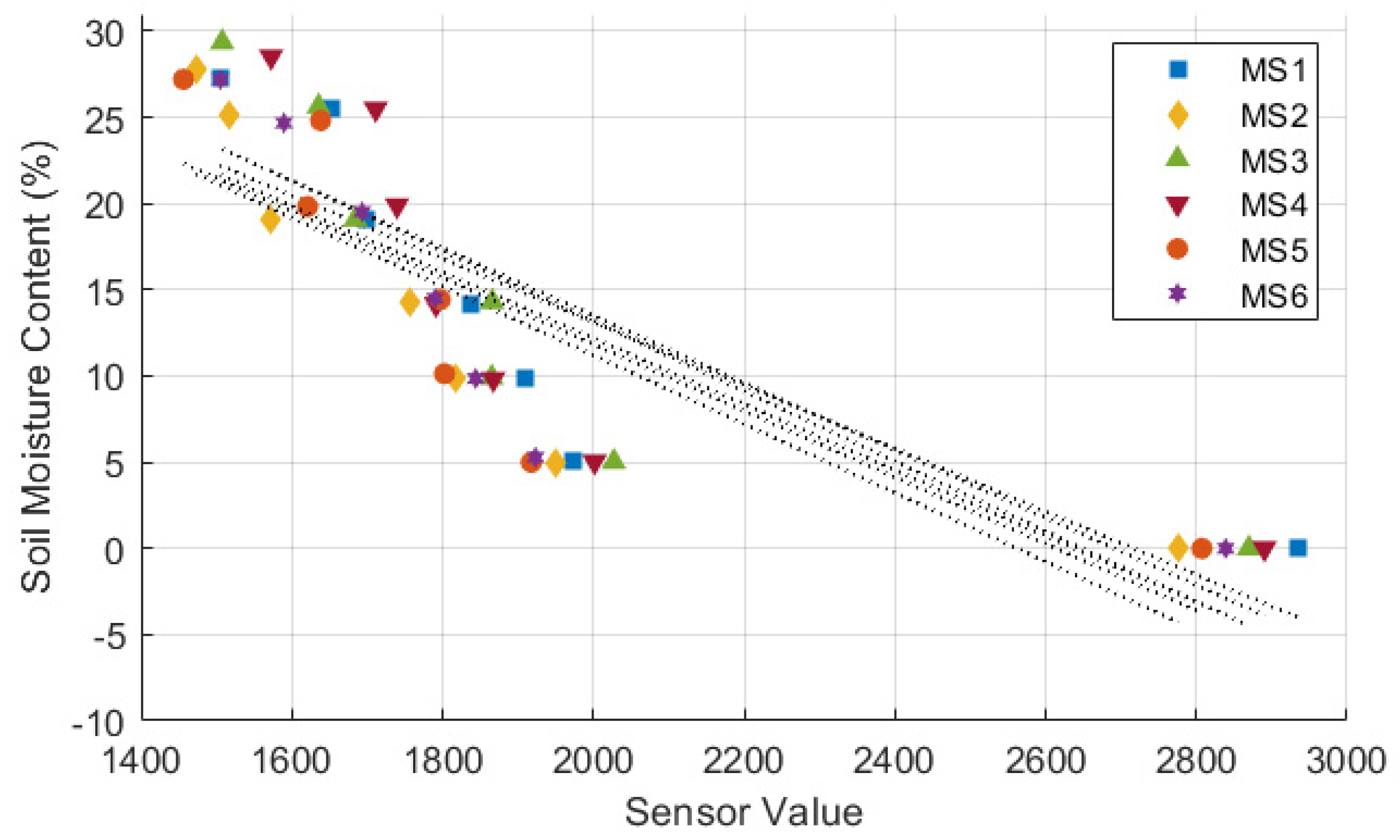
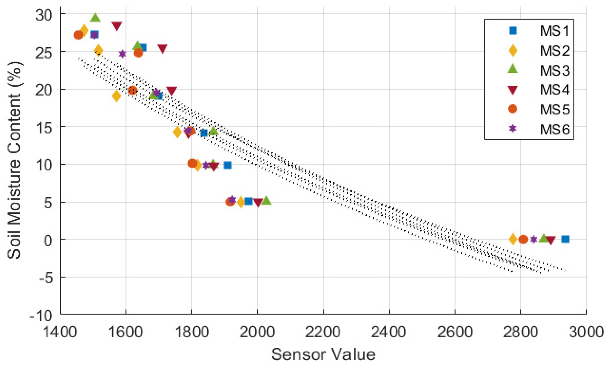
Figure 5,
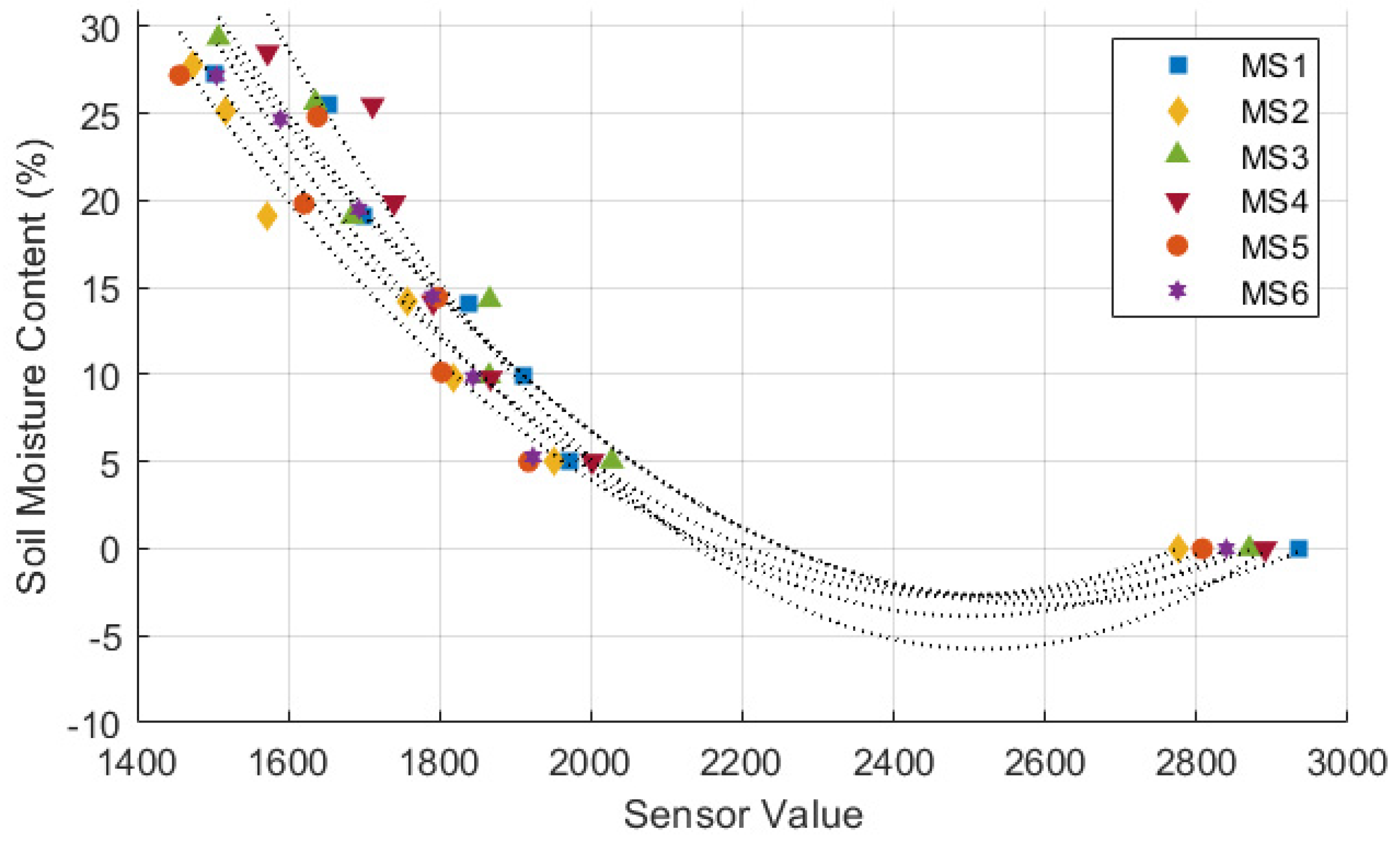
Figure 6 and
Figure 7 illustrates the sensor values obtained from all tested moisture sensors plotted against true soil moisture contents, and the fitting curves of three different types of calibration equation are shown as dotted lines. True soil moisture content refers to the actual moisture content measured from oven-dried samples, as described in step 9 of section 2.2. The calibration lines closely align for all sensors, indicating consistent performance across different sensor units in measuring soil moisture content. Each sensor demonstrates a similar trend but with variations in sensor value readings, suggesting minor differences in calibration or sensitivity among the sensors. The calibration equation results and statistical evaluation of moisture sensors are presented in
Table 3. Statistical analysis reveals that a polynomial equation yields the best calibration results due to its high R
2 and low RMSE compared to other type of equations. Furthermore, data from the calibration process follows a polynomial trend, which can be attributed to a nonlinear behavior of the sensor’s response to changes in soil moisture [
21,
22,
37,
38].
The calibration equation presented in
Figure 7 shows that all sensors had difficulties in measuring moisture content below 5%. Similar cases were observed in previous studies [
39,
40], where some sensors had difficulty in measuring below or above certain values. This issue could be caused by the soil samples were not completely compacted as it will affect the soil-sensor contact. Alternatively, it is possible that the sensor is not sensitive enough to detect moisture at lower soil moisture levels.
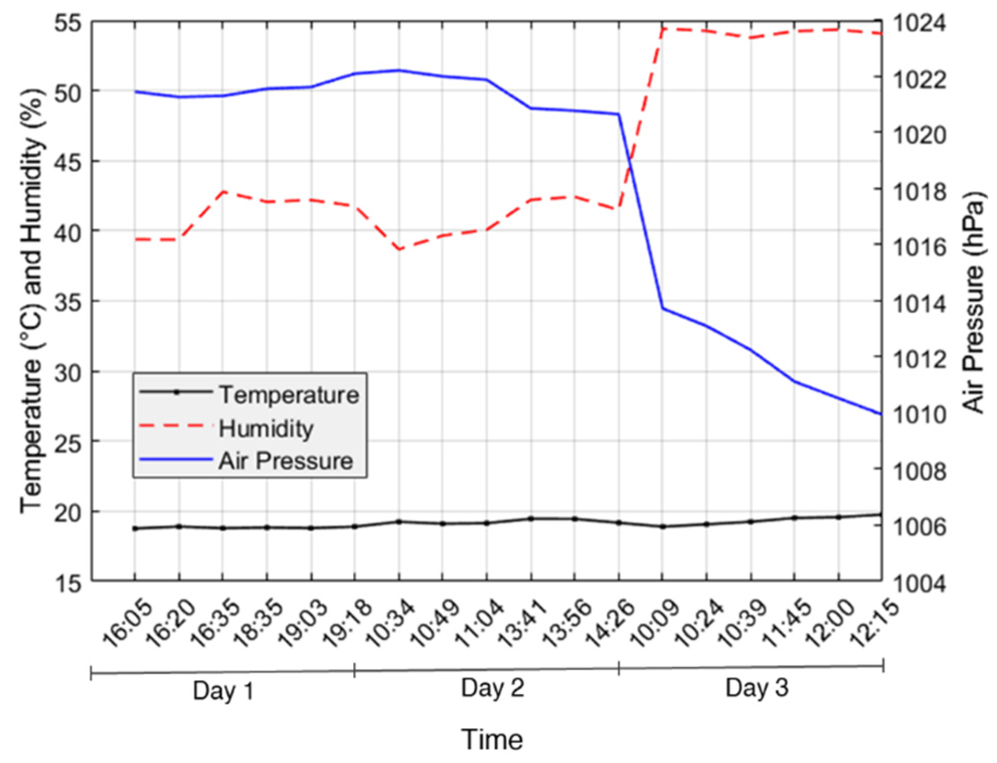
Room temperature, relative humidity and air pressure during the calibration process were shown in
Figure 8 and presented as text axis, which displays label as categories along the x-axis. Calibration process took up three days due to technical issues in the preparation. The room temperature is relatively constant during the calibration process, ranging from 18.7 to 19.7°C. Relative humidity shows an increase, while air pressure decreases over time with a significant drop around the point where humidity sharply rises. This suggests that humidity and air pressure have an inverse relationship: humidity tends to rise as air pressure declines, likely because lower pressure permits the air to contain more moisture. Temperature appears to be less directly affected by these changes, maintaining a consistent trend despite the variations in humidity and air pressure.
3.2. Slope Model Experiment
In slope model experiments, it is essential to assess the fundamental aspects of slope behavior and evaluate the roles played by factors such as geometry, initial and boundary conditions, and soil properties. However, since this study aims to validate the results of moisture sensor calibration equations, the aforementioned aspects are not the focus of this paper.
In this section, moisture sensors were tested in slope model experiments, and the soil moisture contents were observed under different artificial rainfall conditions.
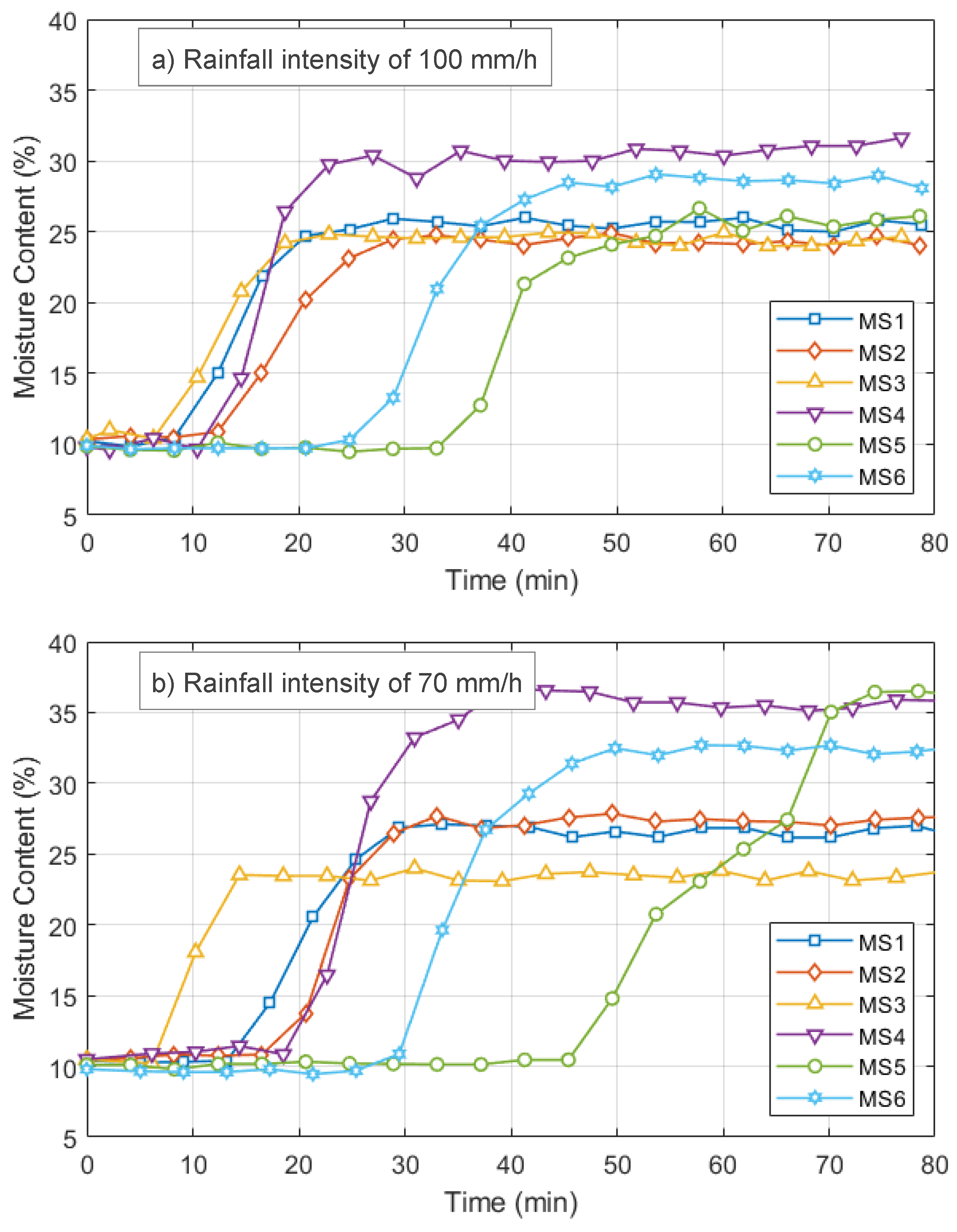
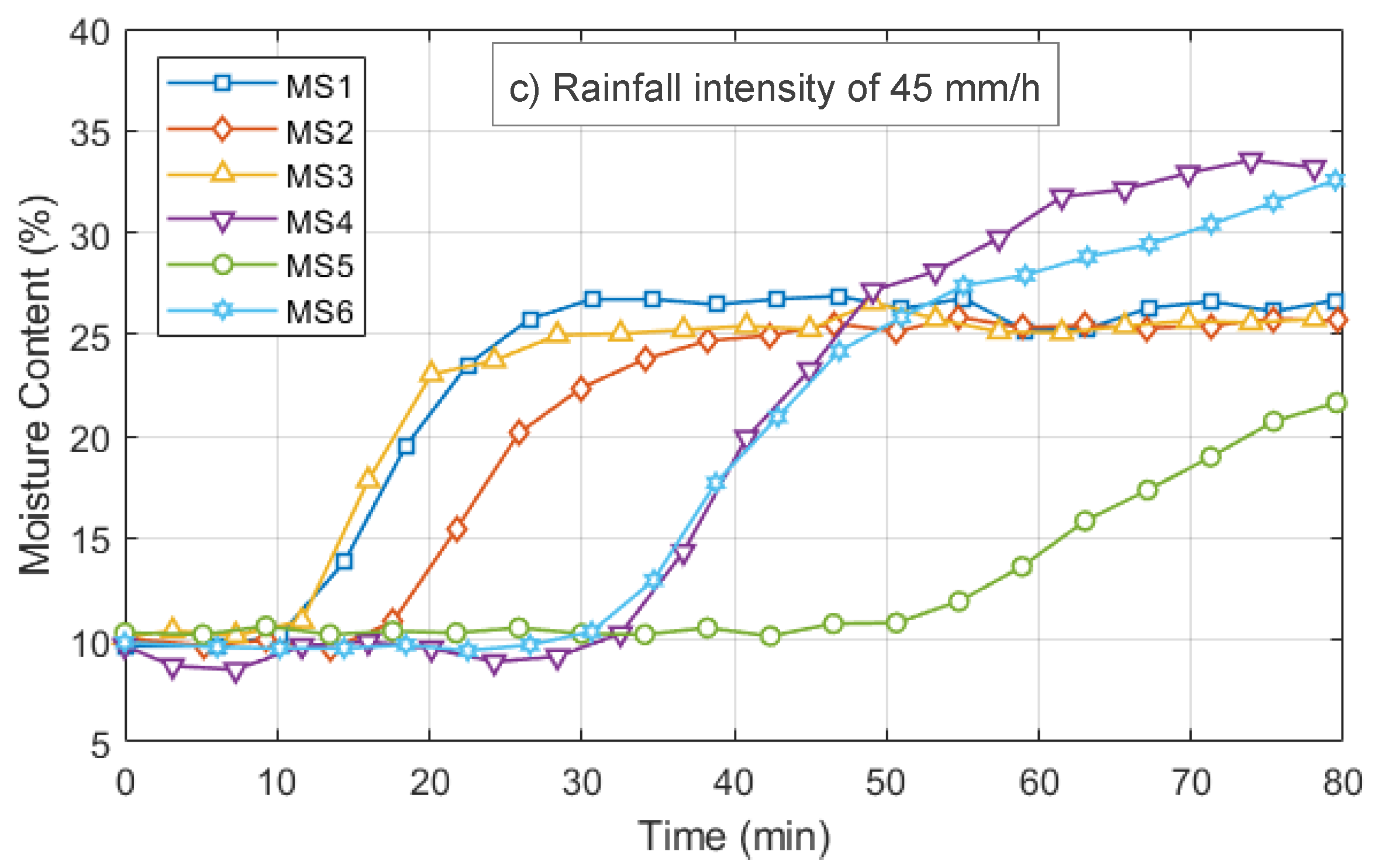
Figure 9 illustrates the changes in subsurface moisture contents recorded by the moisture sensors in response to rainfall over time since the beginning of the experiment. Initially, all moisture sensors recorded a similar moisture content of around 10%. As the soil was subjected to 100 mm/h rainfall (
Figure 9a), moisture sensors near the surface (MS1, 2, 3, 4) recorded an increase in soil moisture content, followed by moisture sensors located further from the surface (MS5 and 6). Within 10 minutes, all moisture sensors located near the surface recorded a change in soil moisture content and reached critical condition within 30 minutes, while MS5 and 6 started to record an increase in soil moisture content within 30 minutes and reached critical condition within 50 minutes. Critical condition in this experiments refer to the condition where the moisture sensors recorded relatively stable of soil moisture content. A similar pattern was observed in slope model experiments under 70 and 45 mm/h rainfall, although lower rainfall intensities resulted in slower moisture detection by the sensors. This demonstrates that rainfall intensity directly influences the response time of the moisture sensors due to rainwater infiltration.
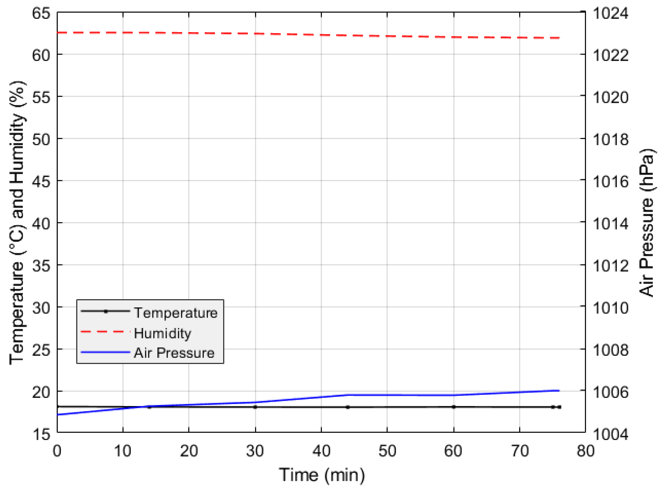
During the slope model experiment, temperature, humidity and air pressure has minor changes as presented in
Figure 10. The temperature remains within a narrow range, with a difference of only 0.06°C, indicating a stable trend. Humidity levels are also stable, consistently around 62%, indicating no significant changes in moisture levels. Air pressure shows slight increase but remains relatively steady, above 1004 hPa. This stability shows that the environmental conditions during the slope model experiment were remain consistent.
4. Discussion
4.1. Moisture Sensor Calibration
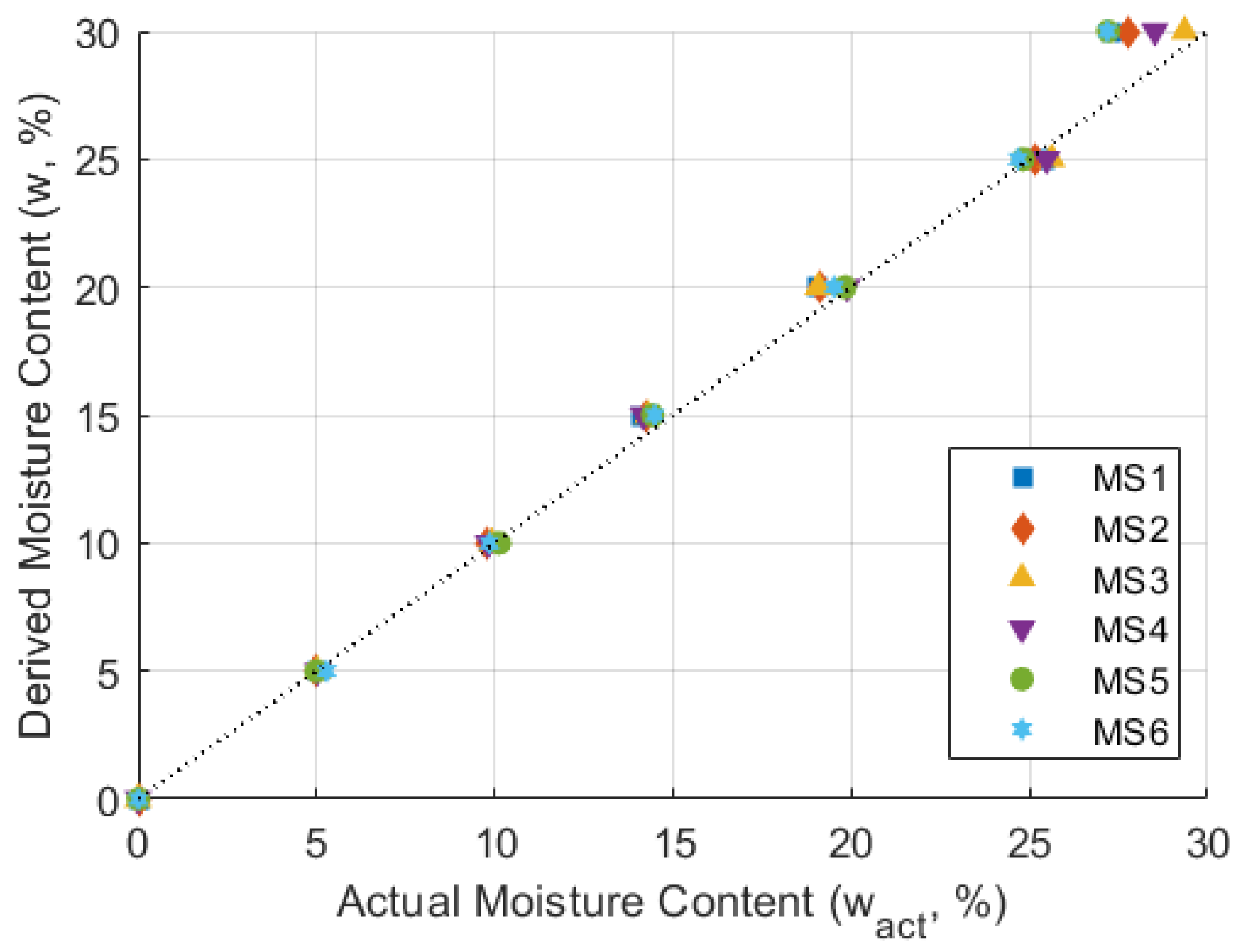
Performance evaluation of soil moisture sensors was conducted in the laboratory settings. Soil temperature during sensor calibration was constant at 16.0 ± 1.4 °C. The comparison of moisture content with actual moisture content is presented in
Figure 11. The derived moisture contents (
) were obtained from the known quantities of water added to the oven-dried soil before the calibration process, while the actual moisture contents (
) were determined by the oven-drying soil samples after the measurement in the calibration process. It is shown that the derived moisture and the actual moisture content are almost identical. However, the values changed when the moisture content exceeded 25%, suggesting that the recorded moisture content deviates when the soil reaches critical condition.
Statistical results reveal that individual sensor calibration using a polynomial equation yielded the lowest R2 of 0.92, the highest RMSE of 2.67, and an MBE of -0.03, whereas the universal or generalized calibration from all sensors produces values of R2, RMSE, and MBE of 0.92, 2.74, and 5.44, respectively. Despite the identical value of R2, the universal calibration exhibited higher RMSE and MBE values. A high RMSE value indicates a significant deviation between the sensor-measured moisture contents and the actual moisture contents, indicating a lack of precision in the model. Furthermore, a positive 5.44 in MBE indicates a significant systematic error in the measurements, suggesting that, on average, the sensor consistently overestimates the actual moisture contents. Therefore, although individual sensor calibrations demonstrated the same R2 values compared to universal calibrations, the higher RMSE and MBE values in the universal calibration highlight greater imprecision and systematic overestimation errors. It is important to note that converting the raw sensor values using universal calibration can lead to inaccuracies when measuring the initial moisture content, despite the consistent trend of increasing moisture content. These inaccuracies are likely due to the inherent variability of individual sensors. Each sensor may have unique characteristics and responses due to manufacturing differences, environmental conditions, and wear and tear. Universal calibration applies a generalized correction that cannot accommodate these individual sensor variances, resulting in systematic error and inaccuracies.
This finding is specific to the tested soil sample and may have different results with different types of soil and conditions [
40,
41]. Previous studies [
37,
39,
42] have consistently emphasized the importance of utilizing a local or individual calibration curve for a specific type of soil rather than a universal calibration approach. The polynomial function of the individual sensor calibration curve demonstrates satisfactory consistency between soil moisture content and sensor value with R
2 greater than 0.90, similar to the correlation found in other studies [
22,
25,
39,
43].
4.2. Sensor Performance in Slope Model Experiment
After the slope model experiment concluded, soil samples were collected to measure the actual soil moisture content (
), which was then compared to the moisture content readings obtained by the sensors
(
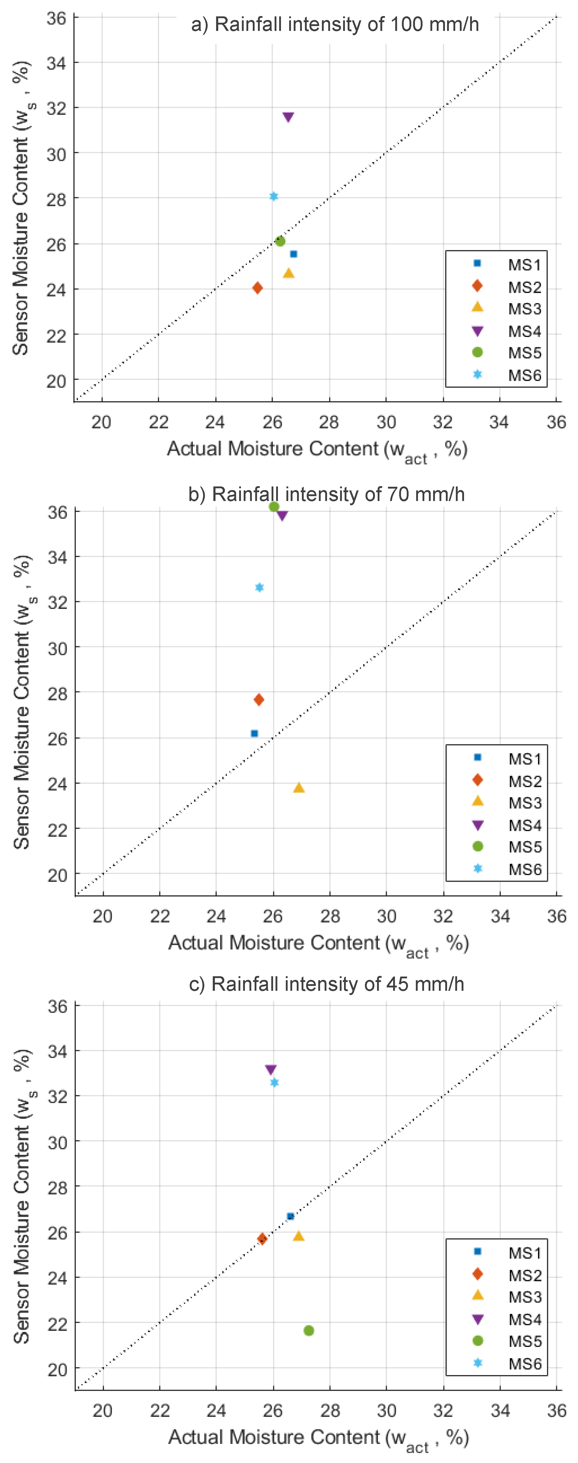
Figure 12). The differences in moisture contents (Δw) are presented in
Table 4. Positive values indicate an overestimation of moisture content, while negative values indicate an underestimation of moisture content by the sensors. The mean bias error of the sensors in the slope model experiment under rainfall intensities of 100, 70, and 45 mm/h are 0.39, 4.43, and 1.20, respectively.
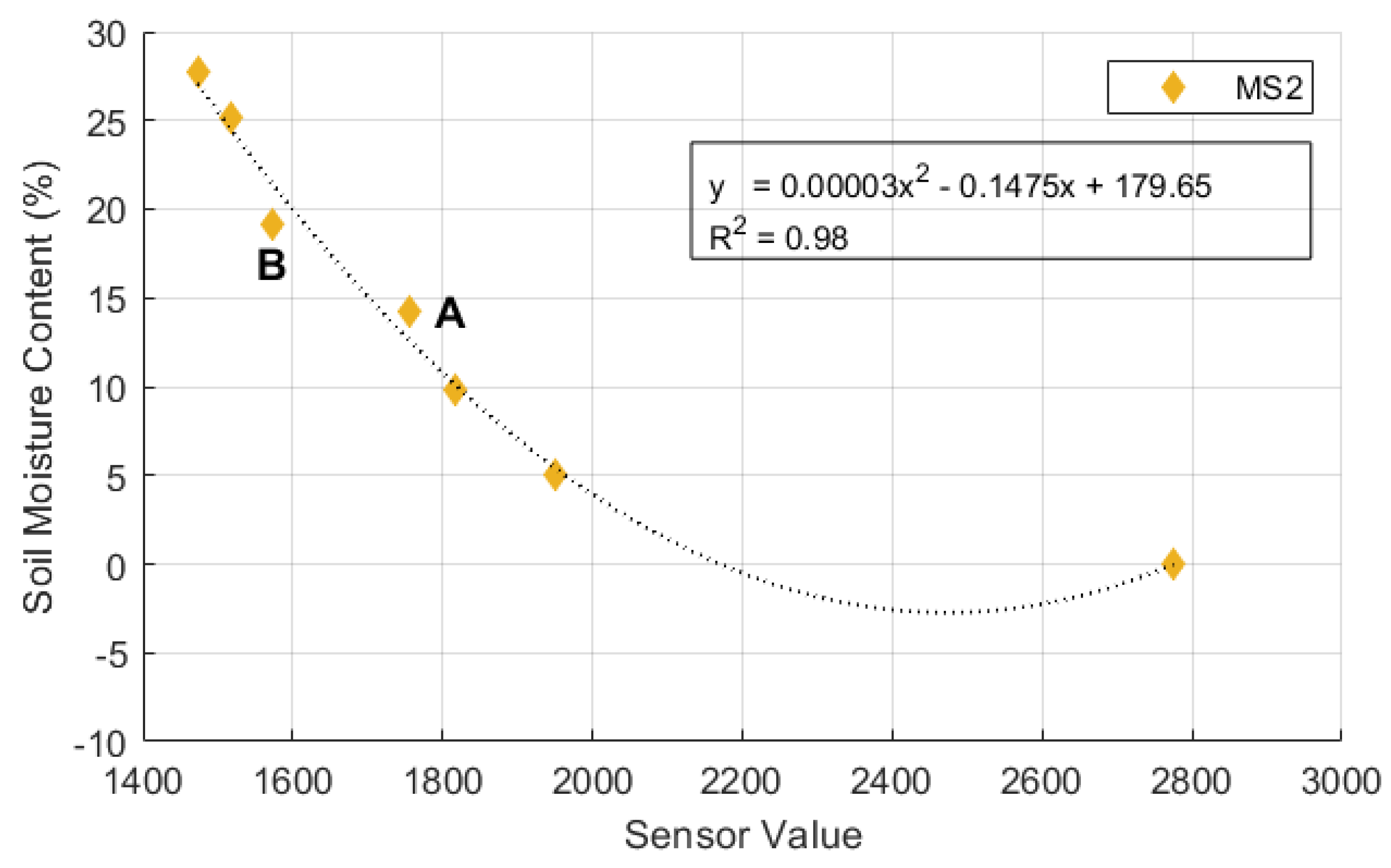
The disparity between the actual and the sensor moisture content (Δw) could be caused by the calibration process and its estimations. For instance, the calibration data of moisture sensor number 2 (MS2) is illustrated in
Figure 13. At point A, the polynomial equation underestimates the moisture content. During calibration, a sensor value of 1757 corresponded to 14.2% of the soil moisture content. However, when using the individual calibration equation for MS2, the same sensor value is equal to 12.5% of moisture content.
On the contrary, the calibration equation overestimates the soil moisture content value at point B. During the calibration process, a sensor value of 1572 corresponded to a soil moisture content of 19.1%, while the calculated moisture content using the polynomial calibration equation was 21.5%. The deviation in sensor readings could reduce the accuracy of the monitoring system. However, in the case of an example presented above, the moisture content difference or error of ±10 % is acceptable given that previous research has already mentioned that this sensor has medium accuracy [
39]. It is important to note that both underestimation and overestimation occur in all moisture sensors, as presented in
Figure 7.
The calibration process and the slope model experiment were carried out around the end of winter, which explains the relatively low temperatures observed. During the calibration process, variations in humidity and air pressure were observed. However, these variables slightly changes during the slope model experiment. This difference can be attributed to the timing of the two experiments: sensor calibration was performed at different times over three days, when air pressure and relative humidity naturally fluctuate, while the slope model experiment was conducted in the middle of the night, when the environmental conditions were more stable [
44,
45]. Overall, these findings emphasize the importance of timing in experimental design, as it significantly impacts the environmental conditions affecting sensor calibration and performance.
The drawbacks of the experiment included, but were not limited to, experimental and human errors, as well as the use of soil with uniform particle size (
Figure 3). Uniform soil, such as coarse sand, has a lower sensor-surface contact area, while fine sand has a higher sensor-surface contact area, both of which affect the sensor readings. Additionally, soil temperature, salinity, and bulk density also influence the sensor values [
46,
47]. Another aspect that was not tested in this research is the durability of the sensor under laboratory conditions. To improve the accuracy of sensor readings and mitigate these issues, several methods can be implemented: 1) Conducting calibration process with different soil particle size, salinity and density; 2) Periodic calibration is crucial, as sensor age can affect reliability [
48]. The calibration of sensor systems, like the interdigital conductance sensor for measuring liquid film thickness, highlights the importance of accurate measurements for system reliability [
49]; 3) Conducting calibration and slope model experiments in a similar environmental settings to improve precision, and; 4) Applying filters such as the Kalman filter helps reduce noise and correct systematic errors in sensor data [
50]. Furthermore, utilizing machine learning algorithms enables analysis of sensor drift, noise and biases over time [
51,
52].
To expand this study, the authors suggest to validate the calibration and accuracy of soil moisture sensors by deploying the system in the field to monitor a real slope. This validation will contribute to a better understanding of sensor behavior in more complex conditions, data stability, durability or life expectancy, and other factors that could lead to data faults [
48]. For instance, moisture sensors deployed in the field may experience higher noise compared to those in a laboratory study [
53]. Therefore, denoising the transmitted data received by the server is important to avoid false alarms in the development of the landslide early warning system. Finally, the authors would suggest maintaining the total construction of the monitoring system as minimal as possible since the system has the potential to be adapted as a landslide early warning system installed across the globe and reduce the impact of disasters caused by landslides.
5. Conclusions
To ensure the accuracy and reliability of low-cost moisture sensor, calibration on specific soil types and properties is important, as the calibration results significantly influence sensor readings. This study evaluated the performance of low-cost soil moisture sensor (SKU: SEN1093) through laboratory experiment. The study began with the calibration of moisture sensors to develop sensor calibration equations and identify the equation that yields the best results. The calibration results were then verified through three slope model experiments using silica sand, with varying rainfall intensities. The following conclusions summarize the key outcomes and implications of this study:
According to the statistical analysis, calibration using the polynomial equation performed best compared to the linier and logarithmic equations. The polynomial equation exhibited the lowest R2 of 0.92, the highest RMSE of 2.67, and an MBE of -0.03.
The developed soil-specific calibration equation for the slope model experiments provided moderate accuracy, yielding a prediction error of ±10%. This prediction error is due to the sensors’ underestimation and overestimation of the actual moisture content.
The study suggests that individual sensor calibration achieves greater accuracy than universal or generalized calibration. Overall, universal calibration exhibited lower R² value, and higher RMSE and MBE, indicating a lack of accuracy and precision in the model.
The calibration process can be influenced by the time of day, when humidity and air pressure naturally fluctuate, whereas the slope model experiment experienced stable nighttime conditions for both humidity and air pressure. This underscores the importance of scheduling or timing to ensure consistent environmental factors in sensor testing.
The use of low-cost moisture sensors integrated with the Internet of Things (IoT) shows its potential to be used for the development of landslide early warning system. It is necessary to have an in-depth slope model research that incorporates all parameters that affecting sensor behavior under different conditions, such as variation in soil temperature, salinity, particle size, and bulk density. Lastly, further studies should be undertaken to assess the sensor behavior in a real-world scenario under field conditions.
Author Contributions
Conceptualization, H.H.; methodology, M.H. and H.K.; formal analysis, M.H.; writing—original draft preparation, M.H.; writing—review and editing, M.H., H.H. and H.K.; supervision, H.H. All authors have read and agreed to the published version of the manuscript.
Funding
Original study was funded by Sabo and Landslide Technical Center, Japan. The study could be further proceeded with generous financial assistance from Japan Construction Information Center (JACIC), Japan.
Conflicts of Interest
The authors declare no conflicts of interest.
References
- Froude, M.J.; Petley, D.N. Global Fatal Landslide Occurrence from 2004 to 2016. Natural Hazards and Earth System Sciences 2018, 18, 2161–2181. [Google Scholar] [CrossRef]
- Saito, H.; Korup, O.; Uchida, T.; Hayashi, S.; Oguchi, T. Rainfall Conditions, Typhoon Frequency, and Contemporary Landslide Erosion in Japan. Geology 2014, 42, 999–1002. [Google Scholar] [CrossRef]
- Schuster, R.L.; Fleming, R.W. Economic Losses and Fatalities Due to Landslides. Environmental & Engineering Geoscience 1986, xxiii, 11–28. [Google Scholar] [CrossRef]
- Guzzetti, F.; Gariano, S.L.; Peruccacci, S.; Brunetti, M.T.; Marchesini, I.; Rossi, M.; Melillo, M. Geographical Landslide Early Warning Systems. Earth Sci Rev 2020, 200, 102973. [Google Scholar] [CrossRef]
- Sorensen, J.H. Hazard Warning Systems: Review of 20 Years of Progress. Nat Hazards Rev 2000, 1, 119–125. [Google Scholar] [CrossRef]
- Ahmadi-adli, M.; Huvaj, N.; Toker, N.K. Rainfall-Triggered Landslides in an Unsaturated Soil: A Laboratory Flume Study. Environ Earth Sci 2017, 76, 735. [Google Scholar] [CrossRef]
- Xu, J.; Ueda, K.; Uzuoka, R. Evaluation of Failure of Slopes with Shaking-Induced Cracks in Response to Rainfall. Landslides 2022, 19, 119–136. [Google Scholar] [CrossRef]
- Chueasamat, A.; Hori, T.; Saito, H.; Sato, T.; Kohgo, Y. Experimental Tests of Slope Failure Due to Rainfalls Using 1g Physical Slope Models. Soils and Foundations 2018, 58, 290–305. [Google Scholar] [CrossRef]
- Liu, Y.; Hazarika, H.; Kanaya, H.; Takiguchi, O.; Rohit, D. Landslide Prediction Based on Low-Cost and Sustainable Early Warning Systems with IoT. Bulletin of Engineering Geology and the Environment 2023, 82, 177. [Google Scholar] [CrossRef]
- Hidayat, M.N.; Hazarika, H.; Fujishiro, T.; Murai, M.; Manandhar, S.; Liu, Y.; Fukumoto, Y.; Kanaya, H.; Takiguchi, O. Evaluation of Landslide Triggering Mechanism During Rainfall in Slopes Containing Vertical Cracks. In Geo-Sustainnovation for Resilient Society; Hazarika, H., Haigh, S.K., Chaudhary, B., Murai, M., Manandhar, S., Eds.; Springer, 2024; pp. 47–56. [Google Scholar] [CrossRef]
- Cogan, J.; Gratchev, I. A Study on the Effect of Rainfall and Slope Characteristics on Landslide Initiation by Means of Flume Tests. Landslides 2019, 16, 2369–2379. [Google Scholar] [CrossRef]
- Huang, C.-C.; Yuin, S.-C. Experimental Investigation of Rainfall Criteria for Shallow Slope Failures. Geomorphology 2010, 120, 326–338. [Google Scholar] [CrossRef]
- Pajalić, S.; Peranić, J.; Maksimović, S.; Čeh, N.; Jagodnik, V.; Arbanas, Ž. Monitoring and Data Analysis in Small-Scale Landslide Physical Model. Applied Sciences 2021, 11, 5040. [Google Scholar] [CrossRef]
- Peranić, J.; Čeh, N.; Arbanas, Ž. The Use of Soil Moisture and Pore-Water Pressure Sensors for the Interpretation of Landslide Behavior in Small-Scale Physical Models. Sensors 2022, 22, 7337. [Google Scholar] [CrossRef] [PubMed]
- Zhao, B.; Dai, Q.; Zhuo, L.; Zhu, S.; Shen, Q.; Han, D. Assessing the Potential of Different Satellite Soil Moisture Products in Landslide Hazard Assessment. Remote Sens Environ 2021, 264, 112583. [Google Scholar] [CrossRef]
- Segoni, S.; Rosi, A.; Lagomarsino, D.; Fanti, R.; Casagli, N. Brief Communication: Using Averaged Soil Moisture Estimates to Improve the Performances of a Regional-Scale Landslide Early Warning System. Natural Hazards and Earth System Sciences 2018, 18, 807–812. [Google Scholar] [CrossRef]
- Ray, R.L.; Jacobs, J.M. Relationships among Remotely Sensed Soil Moisture, Precipitation and Landslide Events. Natural Hazards 2007, 43, 211–222. [Google Scholar] [CrossRef]
- Rawat, P.S.; Barthwal, A. Landslide Monitor : A Real-Time Landslide Monitoring System. Environ Earth Sci 2024, 83, 226. [Google Scholar] [CrossRef]
- Oguz, E.A.; Depina, I.; Myhre, B.; Devoli, G.; Rustad, H.; Thakur, V. IoT-Based Hydrological Monitoring of Water-Induced Landslides: A Case Study in Central Norway. Bulletin of Engineering Geology and the Environment 2022, 81, 217. [Google Scholar] [CrossRef]
- Placidi, P.; Vergini, C.V.D.; Papini, N.; Cecconi, M.; Mezzanotte, P.; Scorzoni, A. Low-Cost and Low-Frequency Impedance Meter for Soil Water Content Measurement in the Precision Agriculture Scenario. IEEE Trans Instrum Meas 2023, 72, 1–13. [Google Scholar] [CrossRef]
- López, E.; Vionnet, C.; Ferrer-Cid, P.; Barcelo-Ordinas, J.M.; Garcia-Vidal, J.; Contini, G.; Prodolliet, J.; Maiztegui, J. A Low-Power IoT Device for Measuring Water Table Levels and Soil Moisture to Ease Increased Crop Yields. Sensors 2022, 22, 6840. [Google Scholar] [CrossRef]
- Kulmány, I.M.; Bede-Fazekas, Á.; Beslin, A.; Giczi, Z.; Milics, G.; Kovács, B.; Kovács, M.; Ambrus, B.; Bede, L.; Vona, V. Calibration of an Arduino-Based Low-Cost Capacitive Soil Moisture Sensor for Smart Agriculture. Journal of Hydrology and Hydromechanics 2022, 70, 330–340. [Google Scholar] [CrossRef]
- Borah, S.; Kumar, R.; Mukherjee, S. Low-Cost IoT Framework for Irrigation Monitoring and Control. International Journal of Intelligent Unmanned Systems 2020, 9, 63–79. [Google Scholar] [CrossRef]
- Nagahage, E.A.A.D.; Nagahage, I.S.P.; Fujino, T. Calibration and Validation of a Low-Cost Capacitive Moisture Sensor to Integrate the Automated Soil Moisture Monitoring System. Agriculture 2019, 9, 141. [Google Scholar] [CrossRef]
- Pereira, R.M.; Sandri, D.; Silva Júnior, J.J. da Evaluation of Low-Cost Capacitive Moisture Sensors in Three Types of Soils in the Cerrado, Brazil. Revista Engenharia na Agricultura - REVENG 2022, 30, 262–272. [Google Scholar] [CrossRef]
- DFRobot Capacitive Soil Moisture Sensor SKU:SEN0193 Available online:. Available online: https://wiki.dfrobot.com/Capacitive_Soil_Moisture_Sensor_SKU_SEN0193 (accessed on 16 May 2022).
- Slyfox 3 in 1 Soil Moisture Meter for Agriculture Available online:. Available online: https://www.amazon.co.jp/-/en/dp/B0C5SWTL78/?coliid=IMXG1A10B6K1R&colid=G4CJWLMA6XDT&psc=1&ref_=list_c_wl_lv_ov_lig_dp_it (accessed on 26 January 2024).
- Tang, J.; Taro, U.; Huang, D.; Xie, J.; Tao, S. Physical Model Experiments on Water Infiltration and Failure Modes in Multi-Layered Slopes under Heavy Rainfall. Applied Sciences 2020, 10, 3458. [Google Scholar] [CrossRef]
- Lourenço, S.D.N.; Sassa, K.; Fukuoka, H. Failure Process and Hydrologic Response of a Two Layer Physical Model: Implications for Rainfall-Induced Landslides. Geomorphology 2006, 73, 115–130. [Google Scholar] [CrossRef]
- Wang, G.; Sassa, K. Factors Affecting Rainfall-Induced Flowslides in Laboratory Flume Tests. Géotechnique 2001, 51, 587–599. [Google Scholar] [CrossRef]
- Wang, F.; Dai, Z.; Takahashi, I.; Tanida, Y. Soil Moisture Response to Water Infiltration in a 1-D Slope Soil Column Model. Eng Geol 2020, 267, 105482. [Google Scholar] [CrossRef]
- Placidi, P.; Gasperini, L.; Grassi, A.; Cecconi, M.; Scorzoni, A. Characterization of Low-Cost Capacitive Soil Moisture Sensors for IoT Networks. Sensors 2020, 20, 3585. [Google Scholar] [CrossRef]
- Domínguez-Niño, J.M.; Bogena, H.R.; Huisman, J.A.; Schilling, B.; Casadesús, J. On the Accuracy of Factory-Calibrated Low-Cost Soil Water Content Sensors. Sensors 2019, 19, 3101. [Google Scholar] [CrossRef]
- Datta, S.; Taghvaeian, S.; Ochsner, T.; Moriasi, D.; Gowda, P.; Steiner, J. Performance Assessment of Five Different Soil Moisture Sensors under Irrigated Field Conditions in Oklahoma. Sensors 2018, 18, 3786. [Google Scholar] [CrossRef] [PubMed]
- Voltage Regulator - XC6206P302MR (65Z5) Available online:. Available online: https://www.sunrom.com/p/xc6206p302mr-65z5 (accessed on 23 November 2022).
- Texas Instruments TLC555 LinCMOSTM Timer Chip; 2019.
- Bircher, S.; Andreasen, M.; Vuollet, J.; Vehviläinen, J.; Rautiainen, K.; Jonard, F.; Weihermüller, L.; Zakharova, E.; Wigneron, J.-P.; Kerr, Y.H. Soil Moisture Sensor Calibration for Organic Soil Surface Layers. Geoscientific Instrumentation, Methods and Data Systems 2016, 5, 109–125. [Google Scholar] [CrossRef]
- Radi; Murtiningrum; Ngadisih; Muzdrikah, F.S.; Nuha, M.S.; Rizqi, F.A. Calibration of Capacitive Soil Moisture Sensor (SKU:SEN0193). In Proceedings of the 2018 4th International Conference on Science and Technology (ICST); IEEE, August 2018; pp. 1–6.
- Schwamback, D.; Persson, M.; Berndtsson, R.; Bertotto, L.E.; Kobayashi, A.N.A.; Wendland, E.C. Automated Low-Cost Soil Moisture Sensors: Trade-Off between Cost and Accuracy. Sensors 2023, 23, 2451. [Google Scholar] [CrossRef] [PubMed]
- Dong, Y.; Miller, S.; Kelley, L. Performance Evaluation of Soil Moisture Sensors in Coarse- and Fine-Textured Michigan Agricultural Soils. Agriculture 2020, 10, 598. [Google Scholar] [CrossRef]
- Li, B.; Wang, C.; Gu, X.; Zhou, X.; Ma, M.; Li, L.; Feng, Z.; Ding, T.; Li, X.; Jiang, T.; et al. Accuracy Calibration and Evaluation of Capacitance-Based Soil Moisture Sensors for a Variety of Soil Properties. Agric Water Manag 2022, 273, 107913. [Google Scholar] [CrossRef]
- Campora, M.; Palla, A.; Gnecco, I.; Bovolenta, R.; Passalacqua, R. The Laboratory Calibration of a Soil Moisture Capacitance Probe in Sandy Soils. Soil and Water Research 2020, 15, 75–84. [Google Scholar] [CrossRef]
- Adla, S.; Rai, N.K.; Karumanchi, S.H.; Tripathi, S.; Disse, M.; Pande, S. Laboratory Calibration and Performance Evaluation of Low-Cost Capacitive and Very Low-Cost Resistive Soil Moisture Sensors. Sensors 2020, 20, 363. [Google Scholar] [CrossRef]
- Howell, J.F.; Sun, J. Surface-Layer Fluxes in Stable Conditions. Boundary Layer Meteorol 1999, 90, 495–520. [Google Scholar] [CrossRef]
- Hughes, M.; Hall, A.; Fovell, R.G. Dynamical Controls on the Diurnal Cycle of Temperature in Complex Topography. Clim Dyn 2007, 29, 277–292. [Google Scholar] [CrossRef]
- Chandel, A.; Swami, D.; Joshi, N. Calibration Complexities: Full-Scale Error Impact and Simultaneous Variation of Salinity, Temperature, and Moisture Content on Sensor Performance in Soil. Environ Dev Sustain 2024. [Google Scholar] [CrossRef]
- Seyfried, M.S.; Murdock, M.D. Response of a New Soil Water Sensor to Variable Soil, Water Content, and Temperature. Soil Science Society of America Journal 2001, 65, 28–34. [Google Scholar] [CrossRef]
- Ni, K.; Ramanathan, N.; Chehade, M.N.H.; Balzano, L.; Nair, S.; Zahedi, S.; Kohler, E.; Pottie, G.; Hansen, M.; Srivastava, M. Sensor Network Data Fault Types. ACM Trans Sens Netw 2009, 5, 1–29. [Google Scholar] [CrossRef]
- Ren, W.; Jin, N.; Wang, T. An Interdigital Conductance Sensor for Measuring Liquid Film Thickness in Inclined Gas–Liquid Two-Phase Flow. IEEE Trans Instrum Meas 2024, 73, 1–9. [Google Scholar] [CrossRef]
- Park, S.; Gil, M.-S.; Im, H.; Moon, Y.-S. Measurement Noise Recommendation for Efficient Kalman Filtering over a Large Amount of Sensor Data. Sensors 2019, 19, 1168. [Google Scholar] [CrossRef] [PubMed]
- Schmidt, J.Q.; Kerkez, B. Machine Learning-Assisted, Process-Based Quality Control for Detecting Compromised Environmental Sensors. Environ Sci Technol 2023, 57, 18058–18066. [Google Scholar] [CrossRef]
- Pereira, M.; Glisic, B. Detection and Quantification of Temperature Sensor Drift Using Probabilistic Neural Networks. Expert Syst Appl 2023, 213, 118884. [Google Scholar] [CrossRef]
- Hidayat, M.N.; Hazarika, H.; Murai, M.; Kanaya, H. Application of Early Warning System for Monitoring Landslide Vulnerability of Slope. In Proceedings of the 7th International Conference on Geotechnics, Civil
180 Engineering and Structures, CIGOS 2024, Ho Chi Minh City, Vietnam, 4-5 April; 2024; pp. 772–780. [Google Scholar] [CrossRef]
Figure 1.
Equipment used: a) moisture sensor, b) soil moisture meter, c) M5Stack Core2, and d) ENV III sensor.
Figure 1.
Equipment used: a) moisture sensor, b) soil moisture meter, c) M5Stack Core2, and d) ENV III sensor.
Figure 2.
Overview of calibration experiment setup.
Figure 2.
Overview of calibration experiment setup.
Figure 3.
Particle size distribution of K7 sand.
Figure 3.
Particle size distribution of K7 sand.
Figure 4.
Overview of slope model and moisture sensor layout.
Figure 4.
Overview of slope model and moisture sensor layout.
Figure 5.
Calibration of moisture sensor using linier equation.
Figure 5.
Calibration of moisture sensor using linier equation.
Figure 6.
Calibration of moisture sensor using logarithmic equation.
Figure 6.
Calibration of moisture sensor using logarithmic equation.
Figure 7.
Calibration of moisture sensor using polynomial equation.
Figure 7.
Calibration of moisture sensor using polynomial equation.
Figure 8.
Temperature, humidity and air pressure during the calibration process.
Figure 8.
Temperature, humidity and air pressure during the calibration process.
Figure 9.
Moisture content monitoring result on different rainfall intensities: a) 100 mm/h, b) 70 mm/h, and c) 45 mm/h.
Figure 9.
Moisture content monitoring result on different rainfall intensities: a) 100 mm/h, b) 70 mm/h, and c) 45 mm/h.
Figure 10.
Temperature, humidity and air pressure during slope model experiment (100 mm/h).
Figure 10.
Temperature, humidity and air pressure during slope model experiment (100 mm/h).
Figure 11.
Comparison of derived moisture content with actual moisture content during calibration process.
Figure 11.
Comparison of derived moisture content with actual moisture content during calibration process.
Figure 12.
Comparison of sensor moisture content with actual moisture content on different rainfall intensities.
Figure 12.
Comparison of sensor moisture content with actual moisture content on different rainfall intensities.
Figure 13.
Calibration equation of Moisture Sensor number 2.
Figure 13.
Calibration equation of Moisture Sensor number 2.
Table 1.
The overall expenditure associated with the implementation of the soil moisture monitoring system (US$ in May 2024).
Table 1.
The overall expenditure associated with the implementation of the soil moisture monitoring system (US$ in May 2024).
| Item |
Quantity |
Unit Cost ($) |
Subtotal ($) |
Total ($) |
| M5Stack Core2 |
3 |
46.90 |
140.7 |
|
| SKU:SEN0193 |
6 |
5.90 |
35.4 |
|
| Slyfox |
2 |
39.15 |
78.3 |
|
| ENV III sensor |
1 |
5.95 |
5.95 |
|
| |
|
|
|
260.35 |
Table 2.
Soil properties of K7 sand.
Table 2.
Soil properties of K7 sand.
| Description |
Value |
| Specific Gravity, Gs
|
2.62 |
| Density of soil, ρt (g/cm3) |
1.51 |
| Dry density of soil, ρd (g/cm3) |
1.40 |
| Maximum dry density of soil, ρd max (g/cm3) |
1.60 |
| Minimum dry density of soil, ρd min (g/cm3) |
1.19 |
| Void ratio, e
|
0.87 |
Table 3.
Calibration equation results and statistics evaluation of moisture sensors.
Table 3.
Calibration equation results and statistics evaluation of moisture sensors.
| Sensor |
Equation Type |
Calibration Equation |
R2
|
RMSE |
| MS1 |
Linier |
y = -0.0183x + 49.779 |
0.71 |
5.06 |
| Logarithmic |
y = -42.14ln(x) + 332.28 |
0.79 |
4.36 |
| Polynomial |
y = 3E-05x2 - 0.1582x + 197.23 |
0.98 |
1.31 |
| MS2 |
Linier |
y = -0.0199x + 51.084 |
0.76 |
4.69 |
| Logarithmic |
y = -43.16ln(x) + 337.9 |
0.83 |
3.92 |
| Polynomial |
y = 3E-05x2 - 0.1475x + 179.65 |
0.98 |
1.17 |
| MS3 |
Linier |
y = -0.0203x + 53.802 |
0.74 |
5.08 |
| Logarithmic |
y = -45.85ln(x) + 360.54 |
0.81 |
4.30 |
| Polynomial |
y = 3E-05x2 - 0.1527x + 193.14 |
0.97 |
1.72 |
| MS4 |
Linier |
y = -0.0196x + 52.613 |
0.66 |
5.65 |
| Logarithmic |
y = -45.38ln(x) + 357.42 |
0.73 |
5.07 |
| Polynomial |
y = 4E-05x2 - 0.206x + 253.52 |
0.95 |
2.18 |
| MS5 |
Linier |
y = -0.0193x + 50.437 |
0.71 |
5.03 |
| Logarithmic |
y = -42.55ln(x) + 333.98 |
0.78 |
4.41 |
| Polynomial |
y = 3E-05x2 - 0.1449x + 179.61 |
0.92 |
2.67 |
| MS6 |
Linier |
y = -0.0191x + 50.47 |
0.72 |
4.94 |
| Logarithmic |
y = -43.02ln(x) + 337.97 |
0.79 |
4.25 |
| Polynomial |
y = 3E-05x2 - 0.1658x + 203.54 |
0.98 |
1.42 |
Table 4.
The difference between sensor and actual moisture content on different rainfall intensities.
Table 4.
The difference between sensor and actual moisture content on different rainfall intensities.
| Sensor |
Rainfall intensity of 100 mm/h |
Rainfall intensity of 70 mm/h |
Rainfall intensity of 45 mm/h |
| ws (%) |
wact (%) |
Δw (%) |
ws (%) |
wact (%) |
Δw (%) |
ws (%) |
wact (%) |
Δw (%) |
| MS1 |
25.5 |
26.7 |
-1.2 |
26.2 |
25.3 |
0.8 |
26.7 |
26.6 |
0.1 |
| MS2 |
24.0 |
25.5 |
-1.5 |
27.7 |
25.5 |
2.2 |
25.7 |
25.6 |
0.0 |
| MS3 |
24.6 |
26.6 |
-2.0 |
23.7 |
26.9 |
-3.2 |
25.8 |
26.9 |
-1.1 |
| MS4 |
31.6 |
26.6 |
5.0 |
35.8 |
26.3 |
9.5 |
33.2 |
25.9 |
7.3 |
| MS5 |
26.1 |
26.3 |
-0.2 |
36.2 |
26.0 |
10.2 |
21.7 |
27.3 |
-5.6 |
| MS6 |
28.1 |
26 |
2.1 |
32.6 |
25.5 |
7.1 |
32.6 |
26.0 |
6.5 |
|
Disclaimer/Publisher’s Note: The statements, opinions and data contained in all publications are solely those of the individual author(s) and contributor(s) and not of MDPI and/or the editor(s). MDPI and/or the editor(s) disclaim responsibility for any injury to people or property resulting from any ideas, methods, instructions or products referred to in the content. |
© 2024 by the authors. Licensee MDPI, Basel, Switzerland. This article is an open access article distributed under the terms and conditions of the Creative Commons Attribution (CC BY) license (https://creativecommons.org/licenses/by/4.0/).
