Tabular Reinforcement Learning for Reward Robust, Explainable Crop Rotation Policies Matching Deep Reinforcement Learning Performance

Georg Goldenits; Thomas Neubauer; Sebastian Raubitzek; Kevin Mallinger; Edgar Weippl

doi:10.20944/preprints202410.2391.v1

Preprint

Article

Tabular Reinforcement Learning for Reward Robust, Explainable Crop Rotation Policies Matching Deep Reinforcement Learning Performance

This version is not peer-reviewed.

Georg Goldenits^*

,Thomas Neubauer,Sebastian Raubitzek,

Kevin Mallinger,

Edgar Weippl

Georg Goldenits^*

,Thomas Neubauer,Sebastian Raubitzek,

Kevin Mallinger,

Edgar Weippl

This version is not peer-reviewed.

Downloads

Views

Comments

Submitted:

29 October 2024

Posted:

30 October 2024

You are already at the latest version

Abstract

Digital Twins’ design frequently incorporates machine learning and, more recently, deep reinforcement learning techniques in order to interpret data and forecast future outcomes based on incoming data. However, because neural networks are typically considered a ”black box” model, doubts over the reliability of the output from deep learning models continue. In our work, we developed crop rotation policies using explainable tabular reinforcement learning techniques. We created five-step rotations, or a succession of five successive crops, to compare these policies to those produced by a deep Q-learning technique. The purpose of the rotations is to maximize crop yields while upholding prescribed planting guidelines and preserving a healthy amount of nitrogen in the soil. We incorporated phenomena related to weather and price fluctuations into the reward signal to account for the potential impact of external factors on crop production. The deployed explainable tabular reinforcement learning methods outperform the deep Q-learning approach regarding collected rewards when the rewards are not perturbed. For the perturbed case, robust tabular reinforcement learning methods outperform the deep learning approach even more while maintaining human interpretable policies. By consulting with farmers and crop rotation experts, we demonstrate that the derived policies are reasonable to use and more resilient towards external perturbations. Furthermore, the use of interpretable and explainable reinforcement learning techniques increases confidence in resulting policies, thereby increasing the likelihood that farmers will adopt the suggested policies. Digital Twins are often intertwined with machine learning and, more recently, deep reinforcement learning methods in their architecture to process data and predict future outcomes based on input data. However, concerns about the trustworthiness of the output from deep learning models persist due to neural networks generally being regarded as a black box model. In our work, we developed crop rotation policies using explainable tabular reinforcement learning techniques. We compared these policies to those generated by a deep Q-learning approach by generating five-step rotations, i.e. producing a series of five consecutive crops. The aim of the rotations is to maximise crop yields while maintaining a healthy nitrogen level in the soil and adhering to established planting rules. Crop yields may vary due to external factors such as weather patterns or changes in market prices, so perturbations have been added to the reward signal to account for those influences. The deployed explainable tabular reinforcement learning methods collect, on average, at least as much reward over 100 crop rotation plans when randomly starting with any crop compared to the deep learning model. For the perturbed case, robust tabular reinforcement learning methods collect similar amounts of reward across 100 crop rotation plans compared to the non-random reward setting, whereas the deep reinforcement learning agent collects even fewer rewards compared to learning on non-perturbed rewards. By consulting with farmers and crop rotation experts, we demonstrate that the derived policies are reasonable to use and more resilient towards external perturbations. Furthermore, the use of interpretable and explainable reinforcement learning techniques increases confidence in resulting policies, thereby increasing the likelihood that farmers will adopt the suggested policies.

Keywords:

Crop Rotation Planning

;

Digital Twin

;

Explainable AI

;

Reinforcement Learning

;

Sustainable Agriculture

Subject:

Computer Science and Mathematics - Artificial Intelligence and Machine Learning

This preprints belongs to the Topic

(World) Heritage Sites and Values in Danger: Climate-Change Related Challenges and Transformation

1. Introduction

Digital Twins are important tools in various critical infrastructures, such as energy production and distribution, food security, healthcare and information security[5,22,23],when aiming to optimise operations and evaluate potential scenarios [18,19]. Digital Twins replicate real-world entities and operations using sensor data and existing domain knowledge. They frequently incorporate machine learning models to simulate scenarios based on this replication[6]. Reinforcement learning is a particularly promising machine learning technique to use in Digital Twins as it can leverage the Digital Twins virtual environment to learn optimal strategies within it [27]. Recent developments have made deep reinforcement learning a promising tool for realising optimisation potential and increasing productivity [15]. Despite its increasing popularity, a significant disadvantage of using deep reinforcement learning to solve these tasks is that their decision-making process might be hard to trace and understand. However, the model’s decisions must be understandable, especially in critical infrastructure security, as they control systems vital to many people. This transparency makes it easier for the users of the models to assess the consequences and opportunities of the current or future situations, to build trust in the decisions made, and, in the event of malfunctions or failures in the system, to investigate the causes. On the part of the model developer, an explainable decision-making process facilitates the maintainability of the models, as weak points or undesirable results can be identified more quickly [25].

Global food production is one critical system that is experiencing increasing pressure towards optimisation as population numbers grow and climate change presents increasingly difficult challenges [7,16,17,31]. An aspect of food production that has yet to see much attention concerning reinforcement learning-based Digital Twins is crop rotation planning [11]. Reinforcement learning-based Digital twins in this work refer to Digital twins that use some form of reinforcement learning as their machine learning model. There is an implementation by Fenz et al. [9], which uses a deep reinforcement learning agent to derive optimal crop rotation policies. Within their virtual environment, the rewards, which are the expected crop yields, are fixed for each crop succession. Using fixed crop yields for each planning step is generally inaccurate in the real world because factors influencing the yields, such as weather, soil nutrient levels and market prices, can vary massively. However, it is necessary to incorporate these fluctuations in the learning process to represent the real world more accurately and to derive more robust crop rotation policies.

Therefore, this work aims to implement a tabular reinforcement learning agent as an alternative to deep reinforcement learning to derive explainable crop rotation policies. The goal is to show that the tabular agents can perform at least equally as well when the rewards for each state-action pair are fixed and outperform deep reinforcement learning when the rewards are perturbed. Moreover, the learning process of the tabular agent will be adapted to be especially suitable for learning with random rewards and deliver reward-robust, explainable crop rotation policies. The collected rewards will be compared as an evaluation measure on the model side. On the application side, domain experts will evaluate the quality of the crop rotations and their resilience towards external perturbations. The goals of this work can be summarised in the following two theses and corresponding research question:

RT1: Tabular reinforcement learning will lead to better explainable policies while maintaining similar model performance to deep reinforcement learning methods when the training is done with non-noisy rewards.
RT2: Noisy rewards in tabular reinforcement learning algorithms will lead to worse model performance regarding collected rewards and make explanations of performed actions less interpretable compared to tabular reinforcement learning algorithms trained on non-noisy rewards.
RQ1: How can reinforcement learning methods help to improve critical infrastructure management in the long term by ensuring accountability, resilience and adaptability?

The work will be structured as follows: First, we summarise work related to this one in Chapter Section 2, before we discuss the employed concepts, techniques and corresponding definitions in Chapter Section 3. Furthermore, we examine the consequences of the violation of the Markov property and how to work around it. We also present the measures to robustify the training process and how the random rewards are set. The experimental design setup is described in Chapter Section 3. In Chapter Section 5, we present the results, which are then discussed in Chapter Section 6. This includes a discussion on the collected rewards and the effects of the robustification measures, as well as the opinions of the domain experts regarding the applicability and resilience of the derived crop rotations. Chapter Section 7 concludes this work, and we present future research directions.

2. State of the Art & Related Work

This section briefly summarises the current state of the art regarding Digital Twins in agriculture and crop rotation planning. Furthermore, it summarises current developments in explainable reinforcement learning and relevant works on random rewards.

Goldenits et al. [11] found that while reinforcement learning-based Digital Twins play an essential role in various agricultural applications, such as pest and disease detection, water and fertiliser management, or greenhouse climate control, crop rotation planning has been a mostly unexplored topic. Furthermore, in most cases, some form of deep reinforcement learning (DRL) was used, which may deliver useful results but lacks the ability to make the decision process explainable.

Two notable exceptions are the works by Fenz et al. [9] and Fenz et al. [10], who introduce a crop successor suitability matrix based on the NDVI score and show that strategies based on that matrix outperform crop rotations that use the Kolbe matrix as a source. Furthermore, in their works, they set up a reinforcement learning environment and used a deep reinforcement learning agent to obtain crop rotation policies. The environment they set up will be the foundation for the tabular reinforcement learning agents presented in this work. In this environment, yield data for 26 crops are available. Furthermore, the successor suitabilities based on the NDVI score are collected, and crop-growing rules contributed by domain experts are included. The agent obtains a negative reward if any rule or unsuitable succession is chosen. For suitable crop successions, the available yield amount will be the reward.

Milani et al. [20] summarise advances in explainable reinforcement learning methods and categorise them based on where the explanations are derived from in the algorithm, dividing them into feature importance, learning process and MDP, and policy level. This work’s findings fall into the last category.

Xu et al. [32] attempt to structure the work on robustness, safety and generalizability by introducing trustworthy reinforcement learning. According to the authors, dealing with noisy rewards is one part of the robustness aspect of trustworthy reinforcement learning, as it may lead to a conservative or bad policy

Another method involves average reward reinforcement learning, as Wang et al. [29] demonstrate. Their core idea is to use a discretised continuous reward space and maintain a confusion matrix containing the probability that a random reward is sampled given the known true reward in a state. In an algorithm they present, the goal is to use this matrix to estimate the true reward and use that for updating the Q-values.

An algorithm that has been used especially in the context of average reward learning is RVI Q-learning. Abounadi et al. [2] study the asymptotic behaviour of this method and show that it converges to an optimal solution.Wang et al. [30] expand on RVI Q-learning by introducing a robust version of it, which they also show to converge to an optimal solution in a non-robust average-reward MDP.

Bellemare et al. [3] also achieved promising results using a Bayesian approach to the noisy reward problem. Instead of using the expected future rewards in the Bellman equation as a target for optimisation, they try to estimate the underlying reward distribution and replace the expected value with it.

A different commonly used approach in reinforcement learning is experience replay. In this approach, the agent is presented with all the rewards and actions it has faced when encountering a state multiple times, thus breaking apart temporal dependencies between them. Generally, the advantage of using experience replay is considered a more stable learning process [1].

3. Methodology

This work aims to use tabular reinforcement learning methods to derive explainable crop rotation policies in a random reward setting. First, we show that tabular methods can match or outperform deep reinforcement learning by comparing the collected rewards for crop rotations derived in the non-random reward setting. This comparison justifies using tabular methods instead of deep reinforcement learning for crop rotation planning. In the next step, random rewards are implemented based on historical crop yield and crop price data in Austria and the data foundation provided by Fenz et al. [9]. Then, the reinforcement learning models with the best hyperparameter settings from the non-random reward setting were trained on the perturbed rewards. To ensure results that are resilient towards these perturbations, the tabular reinforcement learning methods are adapted in the action decision step and the planning phase – in case a technique uses a model. The goal of these adaptations is, on the one hand, to match the performances in the non-random reward setting and, on the other hand, to gain additional insights into the training process. Lastly, the crop rotation policies are evaluated by domain experts to assess how useful the suggestions are and whether the explanations are clear to understand and provide additional confidence in adopting decision support for crop rotation planning.

3.1. Definitions

Digital Twins: The core concept of Digital Twins is that they replicate real-world entities, systems, or organisms in a virtual environment. Michael Grieves published the first use case for Digital Twins in 2003, in which he tried to optimise a factory process by virtually replicating it [12]. Digital Twins often rely on sensor data and expert knowledge to transfer a real system as accurately as possible to the virtual space, thus making them usable in various Internet of Things (IoT) applications.

A key component of most Digital Twins is some form of machine learning model that is used to run simulations within the environment. These simulations aim to create potential scenarios that might, under certain circumstances, be encountered in the real world and serve to guide decision-making for the real-life scenario. In addition, the effects of deliberate changes to a system can be observed, and preparations for unseen scenarios can be made. [6]

Reinforcement Learning: The main goal of reinforcement learning is to find the best course of action among a list of available states and actions in a Markov Decision Process(MDP). That means an agent aims to derive an optimal policy to maximise a reward signal it receives by interacting with the environment. In most cases, like, for example, learning to play Chess [26] or controlling vehicles [28], the collected rewards for a state-action pair are deterministic, meaning that the same action always yields the same reward. However, modelling unknown uncertainties in the real world like this is generally inaccurate. An accurate representation of the real world is crucial for a well-functioning system representation. In the context of reinforcement learning, this means that decisions are made, and the subsequent (positive or negative) consequences are observed. However, as the effects of the same action can vary, in the case of reinforcement learning, this can mean that the optimal actions for a given situation are not learnt. Therefore, resilience to variations in the consequences of actions is essential to the model training process. A robust model increases confidence in decisions and enables the development of optimal action strategies, even in previously unobserved situations.

A key property of a MDP is that the Markov Property needs to be satisfied. That means there are no temporal dependencies between the history of visited states and the current and future states.

Before function approximation to the quality function of each state-action pair based on artificial neural networks (ANNs) in the form of deep reinforcement learning was invented, tabular reinforcement learning was the most common form of reinforcement learning. As the name suggests, a table containing each state-action pair’s quality values is maintained and incrementally updated using the Bellman equation [4]. Given enough training time, tabular agents will find the optimal solution, and by maintaining tables, they allow to derive explanations in the learning process. However, handling large state spaces is computationally expensive due to the need to maintain the tables. [27]

Crop rotation planning aims to derive an optimal sequence of crops to grow in succession. It involves finding suitable planting sequences for cash crops, break crops, and cover crops. The goal is to ensure farmers’ income, break pest and disease cycles, and build soil fertility and health. Crop rotation plans can range from short-term plans of two to three years to longer-term plans of up to ten years or more. These plans are customised to suit the needs of individual farmers or fields and specify which crops to plant and when to plant them [21].

Explainability: An important focus point of this work is the explainability of the behaviour of reinforcement learning agents and the interpretability thereof within a real-life context. Explaining the decision process can be split into two parts. Firstly, explanations that are primarily relevant for the model developer. These include tracking the change of Q-values, which indicate the quality of an action compared to other actions, and recording the development of the optimal strategy throughout the learning process. Observations based on these two approaches help capture the influences of (random) rewards on the overall strategy and the decisions themselves and help identify the algorithm’s strengths and weaknesses. Secondly, the stakeholders are mainly interested in why the reinforcement learning agent suggests certain decisions over others, what results can be expected from a particular strategy, and what potential risks a strategy holds; i.e., interpreting the decision-making within real-life contexts.

3.2. Reinforcement Learning Methods

The general literature on reinforcement learning [27], as well as the literature specifically focusing on agricultural problems [11], contains many different reinforcement learning approaches that can be used to find a solution. This section discusses the models relevant to the crop rotation planning problem.

3.3. Tabular Reinforcement Learning Methods

A set of candidate agents need to be defined as a first step towards improving the crop rotation solution with tabular reinforcement learning methods. Among tabular reinforcement learning methods that are summarised in Table 1, there are generally four groups that can be categorised by two decisions.

Model-based vs. model-free techniques [27]. In model-based methods, rewards for state action pairs visited during training are stored as memories, which enables tracing the learning behaviour but comes at a higher computational cost.
On-policy vs. off-policy reinforcement learning [27]. The difference between these two variants is how the Q value for each state-action pair gets updated. In an on-policy setting, the q-value update is based on the next action reward and under the assumption that the current policy will be followed in the future. In contrast, an off-policy agent updates its q values as if it followed a greedy policy even though it does not.

For this work, three methods were chosen, which are also described in detail in [27]:

A basic 1-step tabular Q-learning method that is off-policy and model-free. This is one of the simplest versions of reinforcement learning and is, therefore, easy to implement. However, it has no internal memory, which might lead to bad results in training on random rewards.
DynaQ is an off-policy and model-based algorithm that is more advanced than the 1-step tabular Q-learning as it combines learning and planning by maintaining a model of the environment. The model, which can essentially be seen as memory, is useful for deriving explainable policies and can ensure good learning results even when rewards for the same state-action pair vary over the course of training. The reason for this is that in addition to the exploration and exploitation phase, there is an additional step in the algorithm that can be influenced to learn good results. Maintaining and updating the model increases the computational cost compared to the 1-step tabular Q-learning.
The Expected SARSA algorithm will be tested as an on-policy alternative. This agent is a model-free variation of the frequently used SARSA algorithm that updates its Q-values based on the average Q-values of future actions. The idea behind choosing expected SARSA over its basic version was that fluctuations based on perturbed rewards might be mitigated by selecting actions based on the expected value.

For all agents, we choose an

ϵ

-greedy policy. After a grid search for each agent, we obtained the best results for parameters

ϵ = 0.5

, discount rate

δ = 0.5

, and learning rate

α = 0.3

for both the DynaQ agent and the expected SARSA agent. The same hyperparameters also gave the best result for the 1-step tabular model, except for the discount factor, which was better at

δ = 0.8

3.4. Markov Property

A key component of each Markov Decision Problem (MDP) and, therefore, reinforcement learning is that the Markov Property [13] is satisfied. This means that the current state is independent of every previous decision or observation. In the case of crop rotation planning, this cannot be true. Deciding on what crop to grow next highly depends on what crops were grown on the same plot before the current one, as they influence soil nutrient levels or what kind of roots remain in the soil. Therefore, the historical information of each plot is essential in order to take the best action in the future.

This problem can also be exemplified by considering a simplified environment where only five crops numbered 1 to 5 exist, and an agent wants to plan a sequence of four crops. Two potential sequences at some point during the training might look like this:

$1 \to 4 \to 3 \to$ ?
$1 \to 5 \to 3 \to$ ?

In both sequences, the current state is "crop 3," and the goal is to plan one more step. All five crops are candidates for the last remaining step in both cases. However, certain rules are in place; for example, there needs to be a break of two seasons before planting the same crop again. Adhering to this rule means that in sequence 1, crop 4 and in sequence 2, crop 5 cannot be used in the next step, thus showing that even though in both sequences the current state is "crop 3", the next decision depends on what happened before the current state occurred, which violates the Markov Property.

One way of dealing with this situation is to work with a partially observable MDP (POMDP)[24]. However, solving POMDPs requires computationally expensive solutions, reworking the existing environment, and, therefore, loses the ability to compare the results to the DQN implementation. Instead, the violation is fixed by expanding the state space and, in doing so, avoiding working on a partially observable MDP (POMDP) and instead working with an MDP. That means instead of working with a 26 x 26 table for each planning step, a

26^{n}

x 26 table must be considered for each planning step n,

n \geq 1

. That is because starting at a random crop, there are 26 potential actions for this crop. This is true for each starting crop and results in 26 x 26 potential states after the first planning step – and 26 potential actions. That means for four planning steps, the agent would have to maintain four tables of the following sizes:

26 x 26
676 x 26
17.576 x 26
456.976 x 26

While these tables are not too large to handle by most systems, they do increase memory usage and lead to longer runtimes when values need to be updated.

However, for this publication, the problem can be mitigated by having the agent explore the entire state space once before learning anything and omitting infeasible crop rotation trajectories from the state space. Trajectories were deemed infeasible if taking an action would result in a domain expert’s rule violation. This also includes eliminating trajectories if a rule was violated at some later point during planning. For example, if four planning steps are required and an action would violate a rule, this trajectory would be eliminated. After exploring the state space "forward" once and deleting the infeasible trajectories, a "backward" control has to be run. After the forward exploration, some actions are left without any feasible successor actions as all trajectories have been eliminated immediately or when they became infeasible at a later planning stage. These states without feasible successors have to be omitted, too, as otherwise, the agent would be able to explore the states but would be unable to plan any further, even though the desired crop rotation length was not reached.

Performing this procedure decreases the state space, so now the table dimensions are:

26 x 26
578 x 26
11.648 x 26
206.002 x 26

3.5. Robustifying Tabular Algorithms

As stated in the Section 2 on the related work, research on robust reinforcement learning strategies usually focuses on experience replay [1], robust algorithms [2,30] or Bayesian learning [3]. While these strategies exist, the goal of altering an existing simple algorithm as little as possible is not meat or unattainable. In the case of experience replay, more robust results are achieved by removing temporal dependencies of states and actions. However, as was discussed in Section 3.4, fixing the violation of the Markov property heavily relies on the exact sequence of states and actions. Regarding robust algorithms, they are specifically developed to deal with reward perturbations but are more difficult to implement and may not necessarily be suitable for developing explainable strategies. Furthermore, they require to estimate many more parameters, increasing the computational costs even more. The Bayesian approach that works on estimating the underlying reward distribution might be interesting for how the random rewards were set up in this work. However, the concept so far has been developed mostly for use in deep reinforcement learning applications as the estimated distribution is used to calculate a cross-entropy loss.

So, instead of expanding on one of these concepts, we identified the algorithms’ exploitation phase as the key contributor to making the results more robust. In addition, using the DynaQ agent model allows altering the planning phase by not using only the last observed reward of a state-action pair in the planning step.

One would consider these robustification strategies here because when agents learn their actions based on fluctuating rewards, these variations might lead to exploring and exploiting a bad strategy by accident. This is particularly problematic when the training is completed, and a suboptimal action has the highest Q-value and is, therefore, suggested by the agent as the best one.

A situation like this is depicted in Figure 1, where the current state is "8" and the potential actions are "10", "11" or "12". As can be seen, in this case, the best action, according to the algorithm, is action 11. However, a brief look at the Q-value trajectory of action 10 indicates that it might, in reality, be the better decision, as the Q-values over the course of the training have been higher and, therefore, they have been used more frequently in the exploitation phase. This could mean that, on the one hand, the agent might truly have discovered a new, better strategy for pursuing action 11 instead of action 10. On the other hand, the fluctuation might have occurred due to the fluctuating rewards, where for action 10, unusually low rewards were observed, whereas, for action 11, they were higher than usual. Thus, the number of updates and the general trend of the trajectory of a specific Q-value hold additional information that has not been used in the training process.

This observation leads to the idea of using a weighted 1-step Q-value prediction to favour strategies that have been explored more frequently and have a positive trend. Regarding the prediction of the next Q-value, the goal is to extract the general trend of a trajectory to determine whether a decrease or increase is the consequence of a newly discovered, better strategy or due to the noisy rewards. Therefore, a simple linear regression model is fit to the last 25 percent of the observed Q-value updates for an action that has been explored frequently. If there were eight or fewer updates to a Q-value, all observations are used for the prediction. The reason for this is that for very short trajectories, taking only the last 25 percent of it captures too little information. If an action has only been explored once, there is no linear prediction; instead, the only observed value is the predicted value.

For the weighting part, let

N_{Q_{i}}

be the number of updates for Q-value

Q_{i}

and

N_{m a x} = m a x (N_{Q i})

for

i \in {1, \dots, N_{s t a t e s}}

. Each predicted Q-value

Q_{i}

is multiplied by a weight factor of

w = \frac{1}{2} * (1 + {((1 + N_{Q i}) / (1 + N_{m a x}))}^{\frac{1}{8}})

In case the maximum Q-value of a decision is negative, instead, the factor was set to w = 2 – w to still be able to wrap an

argmax

function around the scaled Q-values and to avoid distinguishing between two cases.

A major challenge in developing this factor was to achieve a balance between favouring the decision with the most updates and considering strategies that were truly developing into becoming the best decisions but have not been explored that much. To aid the agent in choosing the best decision with respect to that balance, the reasons for this particular factor are:

In the weight w, the fraction gets taken to the power of $\frac{1}{8}$ , thus punishing small differences between $N_{Q_{i}}$ and $N_{m a x}$ less, compared to choosing a larger value in the exponent while still having a reasonably fast decay for larger differences of $N_{Q_{i}}$ and $N_{m a x}$
The factor is bound to the interval $(\frac{1}{2}, 1]$ , which ensures the importance of the Q-values $Q_{i}$ in the decision-making, as bounds of 0 and 1 would almost exclusively base the decisions on the number of observations.
The new argmax function was only used after 75 per cent of the training was done on the regular argmax function because the new argmax still favours more frequently updated decisions. This hinders training initially as exploration is more important, but later in the process, the new argmax helps to improve over regular exploitation.

3.6. Robust Planning

A key strength that is unique to DynaQ within the context of this work is combining exploring and planning using a model of the observed states. In a regular non-noisy reward setting, once a state-action pair is observed, the reward is stored in the model and then used in the planning phase. Introducing randomness changes the reward of each state-action pair every time it is explored. To closely resemble the non-random version of the DynaQ agent, the algorithm was adapted to store the last observed reward for each state-action pair and use that in the planning phase. However, doing this disregards all the other outcomes of a state-action pair and means that the last reward is "the most" correct one going into the planning phase. In the way that the random rewards are set up, this is, in most cases, not true. Therefore, there are two alternative strategies that can be pursued regarding the planning phase and the model.

Firstly, one way to ensure that all rewards to the same state-action pair are of equal importance is to collect all of these rewards and, in the planning phase, randomly select one of them to be used in the planning step.
Secondly, another way of thinking about these rewards and giving equal importance to each of them is to construct an estimator for the mean of the underlying distribution and use this value as a target in the planning phase. Implementing this estimator is simple, as the average of the observed rewards is unbiased for the true sample mean. Using the unweighted average also puts equal importance on each observed reward.

Therefore, three different planning strategies, in addition to the updated argmax function, help to robustify the algorithm’s crop rotation policies.

3.7. Deep Reinforcement Learning Method

This work uses Fenz et al.’s [9] implementation as a benchmark. Therefore, the same Deep Q-network (DQN) that is implemented in the Python machine learning library Keras-rl2 was chosen for the DRL method to solve the crop rotation problem. That means the DQN is not duelling, and double DQN is disabled. Similarly to the tabular agents, the exploration policy is epsilon greedy, and the learning rate is 0.9.

3.8. Setting the Random Rewards

Since the target of the crop rotation plans is to maximise the marginal crop yields, measured in Euro/ha, data containing the variation in yields are of interest. Unfortunately, data for marginal crop yields in Austria is not readily available. Therefore, the marginal yields were reconstructed based on the data given by Fenz et al.[9], available only for the year 2022, crop yield data (t/ha) and market price data, which are both collected by Statistics Austria and available for the past 28 years (1995 – 2023) and 17 of the 26 crops of interest. The missing market price data for broad beans for the first eight and last five years of the time series were imputed based on the changes in market prices for peas because, for the available data, the prices behaved very similarly. In the next step for these 17 crops, the proportion of the marginal yield of the total yield for the year 2022 was determined. The resulting values were then multiplied by the total yield data of all the other years.

This process assumes that total revenue and marginal yield are always in the same proportion, which is probably too strong of an assumption. However, this method still produces yield fluctuations that are strongly correlated to the actual crop yields and, therefore, implicitly capture external perturbations and natural crop yield development.

The marginal yield time series for the remaining nine crops were reconstructed by multiplying the available marginal yields with the average yearly change in marginal yields for all other available crops. That means for the year 2022, the multiplying factor was 1, as it is chosen as the reference year. For the year 2021, the average marginal yields were 25 percent lower, which is why the value from 2022 was multiplied by a factor of 0.75 to simulate the price for 2021. This procedure was carried out over the entire time series and thus completes the base data set on which the random rewards are built.

The empiric distributions of each crop’s marginal yield time series were determined to efficiently use the data. For nine crops, a Kolmogorov-Smirnov Test [14] could not reject the null hypothesis that these marginal yields are normally distributed. For the remaining 17 cases, a Gibbs Sampling scheme [8] was implemented to simulate normal distributions for the mean and variance of the yield to also be able to draw samples from a distribution. Arguably, randomly selecting just from the observed values would have been an option to avoid creating distributions. However, sampling from distributions is advantageous, as a wider variety of values can be sampled, and it is more likely to sample values closer to the mean, thus making the random rewards more resilient towards repeatedly drawing outlier values.

In addition to the distributions, trends over the observed period of time could be observed for most crop yields. Therefore, a linear model was fit with crop yields as the dependent variable and time (in years) as the independent variable. For crops where the trend was significant, the coefficient of the estimator was used to add a time-dependent constant to the crop yield.

4. Experimental Design and Setup

The aim of this work is to plan crop rotations efficiently while accounting for unknown variabilities by introducing randomness into the process. Additionally, as outlined earlier, certain robustifications are necessary to accommodate randomness while ensuring reliable results from the proposed reinforcement learning approach. This led to several experimental setups being evaluated and tested against each other for crop rotation planning.

Overall, there are 26 crops available that can be used in the crop rotation plan. These crops, in particular, were chosen because they accounted for 95% of the crops grown in Austria between 2017 and 2021 [10]. For each pair of crops, the direct successor suitability based on the NDVI score is available, which indicates how beneficial a direct crop succession is. Among these crops, the goal of the plans is to maximise crop yields that the agents receive as a reward, which are a direct consequence of available yield data for each crop as well as the successor suitability. In case, a suitable crop succession is planned, the expected crop yield gets multiplied by a factor of 1.1 or 1.2, depending on how beneficial according to the NDVI score this plan is. Should any of four rules introduced by domain experts be violated or an unsuitable crop is planned, the agent receives a negative reward of

- 2 times highest positive reward

instead, thus discouraging it from that plan. The experts’ rules are:

Soil nitrogen levels must not fall below 0
There is a long enough break before planning the same crop again
There cannot be two root crops in direct succession
A crop can only occur a fixed number of times within a crop rotation plan

The length of the plans was chosen because it allows to plan far enough ahead to estimate influences of the plans on soil nitrogen levels and expected yields. A depiction of the crop rotation planning process can be seen in Figure 2.

Thus, to test tabular reinforcement learning and deep reinforcement learning for crop rotation planning, all agents were tasked to learn optimal five-step crop rotation policies for all 26 starting crops by training over 37.500 training episodes. The number of training episodes was fixed at 37.500 because the DQN model performed best at 150.000 training steps – where one step equals planning one step in an episode. Firstly, the regular non-random rewards for each crop yield are used for each agent and in the second step, these deterministic rewards are replaced by their randomised versions. The observations in that setting motivate the approaches to robustify the training process, and in the last step, the effects of the changes to an algorithm with respect to the learned strategies are studied.

Records during the training process are used for explanatory charts to obtain insights into the tabular agents’ decision-making process. For the deep reinforcement learning model, analyses of the results are possible only after the training is completed.

Domain experts evaluate the crop rotation plans and the respective explanation of the learning processes to validate the results and find avenues for further improvements.

A schematic representation of the experimental design is depicted in Figure 3.

5. Results

In the following, the resulting crop rotation plans from the tabular and deep learning agents in the non-random and random reward settings are presented and discussed. First, the focus lies on the technical side of the results regarding the collected rewards. Secondly, expert opinions and real-world applicability are discussed.

5.1. DRL vs. Tabular RL: Non-Random Rewards

To begin with, we want to demonstrate that tabular Q-learning agents, using the updated larger Q-tables that help to fix the violation of the Markov Property, can match Deep Reinforcement Learning in terms of collected rewards and also deliver better explainable strategies.

5.1.1. Overall Rewards During Training

During the DQN’s training process, the rewards for each episode were stored, and therefore, the success of the training process at each iteration can be tracked. Of course, other metrics, like the loss function, can be used for measuring training success. However, they are unique to function approximations and cannot be used when comparing results to tabular agents.

For the tabular agents, the rewards during training were computed differently to obtain more robust results. After each 500 training episodes, 100 episodes were run, always starting with a different crop, and the best strategies and the corresponding rewards were collected and averaged. As depicted in Figure 4, the results show that all tabular agents learn faster and reach higher rewards during training, indicating a better performance of the crop rotations.

A closer look at the best strategies summarised in Table 2 for each starting crop reveals that DQN is best for 1 starting crop, while the 1-step algorithm performs best for 7 crops, DynaQ for 15 crops, and expected SARSA for 18 crops. These results further strengthen the confidence in the tabular agents since the SARSA agent performs particularly well, but also the very simple 1-step Q-learning approach yields reasonable results. Note that these numbers do not add up to 26 as the agents train independently of each other and can arrive at the same conclusion for the best strategy for a given starting crop.

In general, not all crops are suitable starting crops for rotations; for some, adhering to all expert rules and finding suitable crops is not feasible. But not all crops need to be a good starting point, which is why focusing on the most rewarding strategies also allows to gain insights into the quality of the algorithm results. The DQN agent unsurprisingly also has the lowest maximum rewards, but interestingly, its highest rewarding strategy was found for twelve of the 26 crops. The reason for this is that the agent found two very promising four-step rotations, which were applied to a variety of starting crops. This works in most cases but does not allow for a comparatively high peak performance. Regarding the tabular agents, the expected SARSA algorithm seems to find very specific strategies with great performance, while the DynaQ agent seems to find promising crop rotations for a range of crops overall. The 1-step Q-learning agent is definitely the worst of the tabular agents, but the results are still very respectable.

One of the main reasons for DQN’s underperformance is that fixing the violation of the Markov Property is not easy for this particular use case. Techniques like combining sequences of states into one state and using it as experience replay fail because the goal is to plan one step at a time without fixing the sequences beforehand.

In conclusion, combining the results confirms that tabular reinforcement learning agents can match DQN performance for crop rotation planning and can even outperform them in most cases.

5.1.2. Explainability for non-Random Rewards

Regarding the explainability and interpretability of the obtained results, we see that tabular agents are also favourable compared to the DQN agent, as their design allows to derive explanations of the training process and the results. Each Q-value update for each state-action pair can be stored for the tabular agents during the training phase. This allows to analyse the training process afterwards and gain insights into which decisions were favoured at some point during training. Furthermore, especially in the case of fixed rewards, a notion of convergence can be visually determined, indicating whether the value of certain actions still increases or has already peaked. Figure 5 below depicts the Q-value development for the first action after starting in state 4 for the 1-step Q-learning algorithm.

Two things are of particular interest. Firstly, the value of Decision 10 steadily increased until it seemed to have peaked at a value of around 1500. However, after some time, a better policy following decision 10 was found, and its value increased to around 1800. Secondly, for the current best decision, 11, the training has not been fully completed, as the updates to the Q-value still increase the value.

To gain insights into a broader, chronological picture, the best strategy during each point in training can be tracked for each starting state. Figure 6 shows the strategy development for starting state 4 and the 1-step agent.

While these explanations are useful for developing and improving the model as the state of convergence or the current best strategies can be examined, the plots might not be the most useful to stakeholders. For them, explanations behind decisions or visualisations for yield and nitrogen level might be way more useful. An example of visualising these relations can be seen in Figure 7 – this graph can also be derived from the DQN agent.

The explainability tree, however, depicted in Figure 8, is exclusive to the tabular agents because each step of the training process can be tracked, thus allowing to gain insights at which point in training which decisions were favoured and also why it was favoured.

With this interactive graph, at each point during the decision process, it is traceable which actions violated which expert rule, what the yield of the best decision is, and how it defers from the other decisions that did not violate any rule but were also unsuitable. The mentioned information is available when hovering over the respective squares of the tree.

These graphs show that tabular reinforcement learning for crop rotation is advantageous in terms of the explainability of strategies compared to DQN. This also confirms the first thesis: Tabular reinforcement learning will lead to better explainable policies while maintaining similar model performance to deep reinforcement learning methods when the training is done with non-noisy rewards, as it was shown that tabular agents can outperform DQN in collected reward and in addition add explainability to the decision-making process.

5.2. DRL vs. Tabular RL: Random Rewards

After justifying the use of tabular reinforcement learning by showing its advantages in a non-random reward setting, the next step is to examine how randomised rewards affect the strategies. In general, the idea behind using random rewards is to better replicate the real world by allowing the capture of fluctuations in crop yield that may arise due to market volatility or unpredictable weather patterns, for example. The goal, then, is to find more resilient crop rotation strategies and/or estimate the potential risks of planting a certain crop.

5.3. Overall Rewards During Training

Similar to before, the reward developments during the training phase can be compared as seen in Figure 9. This time, the focus lies on the differences between the same agent’s non-random and random training behaviour. For completeness, the DQN rewards are also shown here. In this side-by-side overview, it can be observed that the non-random strategies perform better, as the average rewards during the training process are higher, which can be seen when comparing the graphs row by row. The reason for that is that fluctuations in rewards lead to fluctuating Q-values, as they are directly influenced by the rewards. Thus, Q-values for good decisions can be lower than they should be, and conversely, for worse decisions, they can be unnaturally high, which misguides the agent in learning the optimal crop rotation plans and, therefore, results in lower average rewards.

Diving a bit deeper into the strategy level again reveals that there are still strategies for each agent that are the same regardless of which rewards have been used. As can be seen in Table 3, for most agents, there are 4 to 8 strategies where the random rewards do not affect the best policy, 11 to 15 starting crops where the non-random rewards produce better policy and a bit surprisingly 7 to 10 strategies they are better when trained on the random rewards. The latter observation can be explained by discovering better strategies when certain rewards are unusually higher or lower than in the other setting. From the table, it can also be inferred that the 1-step Q-learning agent is the most susceptible to discovering better crop rotations, while the random rewards do not lead to a lot of better strategies for the expected SARSA agent. The numbers for the DynaQ agent are between the numbers of the other agents, but the number of equal strategies between non-random and random rewards is higher than that of the other two models. Note that the rewards shown here are as if the strategies were executed on non-random rewards to make the results comparable.

Examining the reasons why some strategies differ reveals that for some starting crops, there was a better strategy at some point during training, but due to randomness in rewards, the quality of the best action was sometimes assessed incorrectly, leading to a worse rotation to be considered the best. An example of such a scenario for the DynaQ agent can be observed in Figure 10, where the strategy corresponding to the highest accumulated rewards was 8, 10, 0, 7, 20 while the best strategy after the training, according to the agent, was 8, 11, 6, 23, 10, even though it had a lower overall reward and a lower overall Q-value. The reason why the agent suggests a worse strategy is that due to fluctuating rewards, crop 11 is preferred over crop 10 in the second planning step, which leads to a suboptimal result. The Q-value development of this state-action pair was used as an example in Figure 1. Note that only the last part of the training process is visualised for better readability. In order to avoid such results and increase the overall model performance, the robustification measures that are discussed in Section 3.6 are implemented.

5.3.1. Update Argmax for Exploration

The effects of the changes to the argmax function on the training of the DynaQ agent are exemplified below. In Figure 11, the reward developments during the training process over 37.500 episodes are compared. The red line indicates the point after which the argmax functions differ. Both to the left and to the right of the red line, there are 500 data points, where one data point is the average over 100 training episodes at this stage of training. For better comparability of the results, all training episodes in both cases started with the same crop. Visibly, there are no huge differences between the two graphs, but comparing some summary statistics as in Table 4 only of the parts to the right of the red line reveals that the new argmax function finds better strategies.

On a decision level, Figure 12 reveals the differences between the two approaches. The three graphs show the Q-value development for all potential actions in state 8, whose final Q-value is positive. Simply put, that means that currently, crop 8 is growing or the last of a previous plan, and one of the crops 10, 11 or 12 is a potentially suitable successor. The leftmost plot shows the Q-value development up to the point where the different argmax strategies take over. In the plot in the middle, the regular argmax function – that was also used up until that point and was depicted in Figure 1 – is continuously used, while in the rightmost plot, the above-described new version is shown. In the case where the regular argmax function was continued, action 11 was explored more frequently as it had the higher absolute Q-value. In contrast, the new argmax version favoured exploring decision 10 as it has been explored more frequently up until that point and also had an overall increasing trend of Q-values, whereas the values for decision 11 stagnated. Thus, the new argmax found the overall better decision here, which led to a better performance of this strategy overall.

5.3.2. Differing Planning Strategies for DynaQ

Comparing the results of the three different planning approaches, which all use the update argmax function, using each of the 26 crops as a start of a crop rotation does not indicate that any of the planning versions is decisively better than the others. The agent that uses the last value for planning delivers the highest rewarding strategies for 16 crops and the worst strategies for 8 crops. In contrast, the agent that uses the average observed rewards in planning finds the highest rewarding strategy in 11 cases and the worst in 13 cases, while the agent that plans from randomly sampling previously observed rewards is the best in 11 cases and the worst in 12 cases. Note that the numbers for best and worst strategies do not add up to 26 as there are ties between the agent’s strategies. As a consequence of these inconclusive results, the final suggestions of the DynaQ agent in the random reward setting will be an ensemble of these three planning versions, where for each crop, the highest rewarding strategy from either of these agents will be suggested.

5.4. Robust Random Reward learning vs. non-Random Reward Learning

In Chapter 5.3, the motivation behind robustifying the learning process was to prevent the agent from choosing a worse strategy than the current best due to reward and, therefore, Q-value fluctuations. Compared to Figure 10, Figure 13 shows that there are cases, such as the one depicted, where this goal was achieved, and a better result was maintained.

Even though improvements to the tested agents were made, randomly selecting rewards for the same state-action pairs still costs some performance in terms of collected rewards. Each previously described robust DynaQ version gets outperformed by training on non-random rewards. However, combining the agents into one ensemble even leads to a better average score compared to its non-random counterpart. The flexibility to adapt two major components, exploration policy and planning, in this fairly simple algorithm compared to the other two tabular reinforcement learning agents allows for the introduction of enough improvements so that the performance increases significantly.

An overview of the achieved average score over all starting crops on the final planning suggestion can be seen in Table 5.

These results can also be seen when comparing different strategies again. In Table 6 below, the same comparison is depicted as in Table 3 in Section 5.3; however, now, the robustification measures are used to train the models on the random rewards.

The most notable thing that can be observed is that the DynaQ ensemble now finds better crop rotations for 11 out of 26 starting crops, and in 10 cases, the strategies are identical to the non-random ones. There are also slight improvements in the 1-step Q-learning algorithm’s strategies; however, for the Expected SARSA algorithm, the robustification approaches did not yield the desired results. The reason for that is, that the Q-value trajectories for the state-action pairs gradually decrease after the initial steep increase. That happens because usually, there are more unsuitable actions for each decision, which come with a negative reward, thus decreasing the expected Q-value over all decisions, which leads to decreasing Q-value trajectories. This decreasing trend seems to collide with the idea of choosing the greatest increase to favour a certain action.

Importantly, it has to be noted that obtaining a lower model performance when comparing learning on perturbed rewards to learning on deterministic rewards is not necessarily a negative sign with regard to the model domain. The reason for that is that deterministic rewards might be an idealised but unrealistic representation of the real world, and thus, the rewards may be better on paper but produce worse results when trying to implement them.

5.4.1. Summary

We outlined and extensively discussed the results obtained from our experiments in the previous part of this section. Here again, we briefly summarize our findings with respect to performance and expandability according to the pipeline depicted in Figure 3.

Initially, three tabular reinforcement learning algorithms, 1-step Q-learning, DynaQ and Expected SARSA, were tested against a DQN model to predict 5-step crop rotation policies among a corpus of 26 available crops. We showed that the tabular methods collected more rewards for the obtained crop rotations, thus underlining a superior performance. Furthermore, due to their tabular nature, better explanations of the training process and the results can be obtained, which greatly increases the understanding of why the agents made their decisions.

We also showed that using randomised rewards, which aim at better replicating the real world, negatively impacts the performance of all tested models. To improve the results of training on the random rewards and to obtain more resilient crop rotation plans, robustification measures were taken. These include the proposed changes to the argmax function to encourage the agent to stick to well-explored decisions and the discussed changes to the planning phase of the DynaQ agent, which resulted in three different DynaQ versions. The robust planning increased the model performance of the 1-step Q-learning algorithm and greatly increased the performance of the DynaQ approach when combining the three different models into an ensemble. However, the Expected SARSA algorithm did not show signs of improvement for favouring strategies trained on random rewards.

5.5. Domain Expert Evaluation

To test how the results could uphold in the real-world domain, experts David Mayer, farmer and consultant at the Organization of the Austrian Chamber of Agriculture in Lower Austria (ger.: Landwirtschaftskammer Niederösterreich), Annika Mayer, from BOKU Vienna, Martin Auer, a farmer in Lower Austria and Simon Zoubek, an organic farmer from Biohof Adamah, kindly took their time to validate the results. The focus of the evaluation was to answer whether crop rotations suggested by learning with random rewards are preferable overall and more resilient regarding crop yields compared to those learned with deterministic rewards. Additionally, the evaluation focused on prior experiences with AI in crop rotation planning and whether explanations of the agent’s decision-making process would encourage farmers to adopt these decision-support tools to tools without any explanations. Lastly, the experts were asked to voice concerns and opportunities for using AI in crop rotation planning.

Regarding prior experiences with crop rotation planning and AI, all experts currently use crop rotations on their farms; however, none of them uses any software or AI tool to create the rotation plans. The reasons why no software is used are that prior experience is available, there is no interest in investing time to learn it, and there is no knowledge of any existing product that would do that.

To determine which crop rotation is better to use, the experts were asked to choose their preferred strategy for six different starting crops (Spring Barley, Grain Peas, Grain Maize, Summer Oat, Potatoes and Winter Rye). The starting crops were chosen because they cover root crops, grains, and legumes and because highly rewarding strategies were found for those crops. For each crop, up to three different strategies could be chosen: one was derived from a non-random DynaQ agent, one from the random DynaQ ensemble and in the case where three options were possible, the majority vote of all models was chosen too. The optimal strategy was the same for potatoes for both the non-random and noisy rewards. The experts did not know which crop rotation was derived from which agent in order to avoid biases in any direction. For Spring Barley, Grain Maize and Winter Rye, the suggested strategy learned on the non-random rewards scored higher, and for Grain Maize and Grain Peas, the random reward strategy collected more rewards. Therefore, cases where the experts chose a lower rewarding strategy over a higher one are of particular interest as based on those, more insights into improving the model can be gained. In addition, based on a Likert scale, the experts answered how income resilient towards external perturbations they deemed each strategy to be (not only their preferred one). The possible options on the Likert scale are: 1: not risky at all, 2: not risky, 3: acceptable, 4: risky, 5: very risky.

The results of the interviews regarding the preference of each crop rotation are summarised in Table 7. Interestingly, for the three starting crops where the better strategy was obtained in the deterministic reward setting, the experts’ choice was mixed. In the case of spring barley the random strategy was deemed more suitable because it better adhered to the principle that root crops and stalk plants should alternatingly be planted. Furthermore, according to one expert, the plan is useful for growing crops to feed cattle. However, they also found the perturbed reward strategy useful, especially in the context of organic farming. Another expert preferred the non-random strategy because lucernes grow over multiple years and, therefore, cover the soil over a longer period of time.

The opinions on the strategies for grain maize vary a lot. For the organic farmer, it is important that the lucernes are present in the rotation as they loosen the soil. In contrast, one expert liked to use pumpkins in the rotation. In the case where none of the strategies was preferred, both were deemed impractical as the root material of the soybeans hinders the growth of the pumpkin crops and for the second option, lucernes are not economically feasible.

Again, the alternation between root crops and stalk crops was preferred for the available strategies for winter rye in the random strategy. The reasons for choosing the non-random suggestions are that soybeans are sought after, and for the organic farmer, the random strategy had too much wheat in suboptimal crop breaks.

Compared to the crop rotations plans that were more rewarding in the non-random setting, the opinions on the plans that performed better in the noisy reward setting are way less divided.

For grain peas, all experts agreed on the same plan, as this is a known plan for two farmers. For the organic farmer, peas, in general, are a promising organic culture, and again, he liked that Wheat is grown before potatoes as it requires less work on the soil and, therefore, allows for some regeneration.

Lastly, for summer oats, the random strategy prevailed, as it twice contained some form of Wheat, avoided the aforementioned difficulties for soybeans and pumpkin, and was economically the most promising. Refilling soil nutrients is of greater importance only for the organic farmer, which is why he preferred growing clover, which is suggested by the majority of all models, excluding the DynaQ ensemble.

Regarding the economic risk of the strategies, it is no surprise that the preferred strategy was also seen as the less risky one, as economic considerations play a crucial role when deciding on a crop rotation. In Table 8, an overview of the risk assessment of the preferred strategy is shown, which indicates that most crop rotation plans are deemed acceptable or not risky. Only for grain maize, the plans were seen as very risky, which also coincides with the answer of the expert that none of the plans is feasible.

Overall, the risk assessment aimed at answering the question of whether the crop rotations are seen as resilient towards external perturbations like weather influences or market price fluctuations. According to the answers given, the strategies are resilient enough that they mostly come at an acceptable economic risk. This again emphasises the importance of using the random rewards as present in this work, as nine of the plans preferred originate from training on random rewards, compared to only five choices for plans derived from deterministic rewards.

To examine the importance of explainable AI decision support tools, the experts were shown a sample explainability tree, like in Figure 8 and the soil nitrogen and yield development Figure 7 and concluded that they could determine why the agent made its decision. They also said that such explanations generally increased the chances of AI tools being adopted in crop rotation planning. One expert, however, was sceptical about using AI for their farming operations, and even explanations would not convince them to adopt such decision-support tools. In contrast, one expert was very impressed, especially by the line chart, as they reasoned that crop yields are eventually what economically sustainable farming boils down to, which is why having the ability to somehow estimate the potential future yields is essential. Furthermore, nutrient development is also a key factor for deciding on a crop rotation plan, especially in organic farming, when fertiliser usage is not easily possible.

At the end of the interviews potential concerns as well as future opportunities about using AI for crop rotation planning could be voiced. One major concern with respect to AI tools is that people blindly follow the suggestions without considering potential consequences. Furthermore, there are doubts that AI will ever know a plot as well as a farmer’s and will, therefore, lead to worse decisions.

However, the experts also see a great opportunity to develop AI tools for crop rotation planning. An idea that they came up with in one interview is to develop an app where farmers can enter the crops they want to grow and on which plot of land they want to grow it. Based on the input crops and plot history, a crop rotation plan is created that may be AI-powered and includes explanations such as the one presented in this work that not only considers suitable crop successors but also regulatory needs, potential funding sources, and cover crops. In addition, real-time market price data of crops should be considered, as they are sometimes known for some years in advance.

In general, a lot was talked about the scale on which such AI models could be applied. Frequently, in the interviews, it was concluded that farming practices are very region-dependent as weather conditions, soil nutrient levels, the slope of the field as well and elevation above sea level all contribute to crop growth and, in addition to market price data, influence the final yield. In all interviews, the farmers found that if this information is available, AI would be able to handle it and contribute to their crop rotation plans.

6. Discussion

In our study, we conducted a series of experiments and interviews to explore the potential of tabular reinforcement learning models in crop rotation planning. Our investigation encompassed two primary threads: a technical analysis of their performance under varying conditions and expert interviews to evaluate the practical application of these models in real-world scenarios. The following discusses insights gathered from the comparison of the different reinforcement learning approaches, the conducted interviews, and the key findings that highlight the potential and limitations of AI for planning crop rotations within the given context.

Our experiments demonstrated how our tabular reinforcement learning approaches compare to deep reinforcement learning approaches. We examined how both approaches handle variability in the observed system by introducing noisy rewards, how tabular reinforcement learning approaches can be robustified under these conditions, the differences between these approaches, and how these differences can be interpreted in a real-life context.

Furthermore, the conducted interviews revealed that the presented reinforcement learning models, particularly those trained on random rewards, can be used to model reasonable, resilient, and explainable crop rotations. Although none of the experts interviewed currently rely on software or AI tools for creating crop rotation plans, two of them acknowledged the potential of using such technology in the future, especially when explanations of the decision-making process and the potential consequences of the plans are provided. While this demonstrates the potential of using AI in crop rotation planning, further improvements are needed, such as incorporating additional soil data for organic farming, using funding information, and enabling the model to predict crop rotations on an individual field level to fully unlock AI’s potential in this domain.

In summary, the main takeaways from our experiments and the conducted interviews are:

A more accurate real-world representation of crop yields, modelled by randomised rewards in the learning process, decreases the quality of crop rotation policies learned by reinforcement learning agents.
Robustification measures guide the agents towards overcoming some of the negative influences of the noisy rewards and, therefore, lead to better and more resilient crop rotation plans.
The interviewed domain experts overall favoured the crop rotation plans obtained from the noisy reward training, indicating that accounting for external factors that influence crop yields improves the quality of the crop rotation plans.
Explanatory graphics, such as the ones presented in this work, are deemed necessary by the domain experts to understand why a crop rotation plan was suggested and what effects on the income and the field following that plan has.

Even though related work in agriculture frequently employs DRL methods, tabular reinforcement learning should not be disregarded when explainable decisions are desired. As the interviews showed, explanatory mechanisms in machine learning greatly contribute to gaining trust in decision support tools and to assessing risks that suggested crop rotation plans have.

Furthermore, stakeholders and users of the crop rotation plans are mainly interested in how well a crop rotation fits their agricultural and economic needs. Therefore, efforts such as modelling uncertainties through noisy rewards and then dealing with their effects on the learning behaviour are necessary to make these models attractive for real-world applications. Another contributing factor to increasing interest in these models is to allow for individualised crop rotation planning that can be enabled through means such as the app mentioned before.

Tabular reinforcement learning is a powerful machine learning tool that we have shown and can encompass both of these desires. It can deal with reward perturbations and still deliver crop rotation plans that farmers want to use, which mostly come at an acceptable degree of risk. Moreover, tabular reinforcement learning can deliver the desired explanations, thus making its use easier and more approachable for its users. Another advantage of using reinforcement learning in the crop rotation planning problem is that it allows for the optimization of multiple targets at the same time. The relation between these targets does not have to be known in advance. In general, it suffices to reward behaviour that leads to the desired outcome and punishes undesired crop rotations. For example, an organic farmer might want to have crop rotations focused more on retaining soil nutrient levels over the course of multiple years while still gaining acceptable profits. A farmer that uses fertiliser, on the other hand, might favour profits over all other factors. The main challenge in achieving various goals at the same time is to appropriately set the rewards such that they aid the learning process in the desired direction.

7. Conclusion & Future Research

This work showed that the tabular reinforcement learning agents Q-learning, expected SARSA and DynaQ can outperform a DQN implementation for a crop rotation problem in both the classical deterministic reward setting and for noisy rewards. Furthermore, it was shown that introducing perturbations to collected rewards decreases the model performance. However, measures such as using weighted Q-values and different approaches in the DynaQ planning step can mitigate the effects of the random rewards. The evaluation done by domain experts revealed that explainable AI tools increase the trust decisions they suggested and, therefore, the chance of them being used in crop rotation planning. Moreover, the evaluation showed that random rewards in crop rotation planning contribute to obtaining better plans and that these plans are more resilient towards external influences on crop yields.

While this work contributes to improving reinforcement learning-based crop rotation strategies by increasing model performance and making them more explainable for the model developer and the stakeholder, there is still room for further improvement. As for most machine learning problems, additional data such as soil potassium and phosphorus could contribute to more accurate crop rotations as these soil nutrients ensure healthy crop growth. Furthermore, other learning objectives could be targeted, such as minimising the number of crops in a rotation or aiming for plans that naturally maintain soil nutrient levels. The introduction of random rewards also allows to aim for crop rotations that minimise the yield variance and thus again put emphasis on resilience.

Acknowledgments

The authors acknowledge the funding of the project "digital.twin.farm" funded by the Austrian Federal Ministry of Education, Science and Research. The authors want to thank David Mayer, Annika Mayer, Martin Auer and Sebastian Zoubek for taking the time to answer the questionnaire.

Appendix A

Questionnaire: German Version

Fragebogen: Fruchtfolgeplanung

Name:

Namentliche Erwähnung in der Arbeit: JA □ NEIN□

Tätigkeit/Beruf:

Firma/Organisation:

Fragenblock 1: Persönlichen Erfahrung mit Fruchtfolgeplanung

Arbeiten Sie aktuell mit wechselnden Fruchtfolgen?

JA □ NEIN□
Verwenden Sie bereits bestimmte Programme oder künstliche Intelligenz (KI) zur Unterstützung bei der Fruchtfolgeplanung?

JA □ NEIN□

(a)

Wenn ja, welche Programme oder KI verwenden Sie?

(b)

Wenn ja, wird bei dem Programm oder der KI der Entscheidungsprozess erklärt?

(c)

Wenn nein, was sind die Gründe, warum Sie keine KI oder andere Software verwenden?

Fragenblock 2: Fruchtfolgen, die von unseren Modellen bestimmt wurden

Das Ziel der Fruchtfolgen ist es, das erwartete Einkommen pro Hektar unter Einhaltung gewisser Regeln (z.B.: Stickstoffgehalt im Boden) zu maximieren. Für die Berechnung der Fruchtfolgen wurden 2 Fälle unterschieden:

Das erwartete Einkommen pro Hektar für eine Pflanze verändert sich nicht von Jahr zu Jahr = Risiko nicht berücksichtigt
Das erwartete Einkommen pro Hektar für eine Pflanze unterliegt gewissen Schwankungen, die z.B. durch das Wetter hervorgerufen werden können = Risiko berücksichtigt

Im Folgenden sind beispielhaft einige Fruchtfolgen angeführt, die von meinen Modellen erzeugt wurden. Es gibt 6 verschiedene Startpflanzen. Pro Startpflanze werden entweder 3 oder 2 Fruchtfolgen verglichen bzw. Ihre Meinung zu einer bestimmten Fruchtfolge gefragt. Der Zeitraum der Fruchfolgeplanung liegt immer bei 5 Jahren.

Startpflanze: Sommergerste

A: Sommergerste → Luzerne → Ölkürbis → Winterweichweizen → Kartoffeln

B: Sommergerste → Winterweichweizen → Kartoffeln → Winterdinkel → Linsen

Welche dieser Strategien würden Sie bevorzugen? A □ B □

Warum?

Wie riskant ist Strategie A in Bezug auf das erwartete Einkommen gegenüber externen Einflüssen (z.B. Wetterschwankungen) auf einer Skala von 1 bis 5?

1:gar nicht riskant□, 2:nicht riskant □, 3:akzeptabel □, 4:riskant □, 5:sehr riskant □

Wie riskant ist Strategie B in Bezug auf das erwartete Einkommen gegenüber externen Einflüssen (z.B. Wetterschwankungen) auf einer Skala von 1 bis 5?

1:gar nicht riskant□, 2:nicht riskant □, 3:akzeptabel □, 4:riskant □, 5:sehr riskant □

Startpflanze: Körnererbse

A: Körnererbse → Winterdinkel → Hanf → Winterroggen → Hanf

B: Körnererbse → Wintertriricale → Ölkürbis → Winterweichweizen → Kartoffel

C: Körnererbse → Wintertriricale → Buchweizen → Sommerhafer → Winterweichweizen

Welche dieser Strategien würden Sie bevorzugen? A □ B □ C □

Warum?

Wie riskant ist Strategie A in Bezug auf das erwartete Einkommen gegenüber externen Einflüssen (z.B. Wetterschwankungen) auf einer Skala von 1 bis 5?

1:gar nicht riskant□, 2:nicht riskant □, 3:akzeptabel □, 4:riskant □, 5:sehr riskant □

Wie riskant ist Strategie B in Bezug auf das erwartete Einkommen gegenüber externen Einflüssen (z.B. Wetterschwankungen) auf einer Skala von 1 bis 5?

1:gar nicht riskant□, 2:nicht riskant □, 3:akzeptabel □, 4:riskant □, 5:sehr riskant □

Wie riskant ist Strategie C in Bezug auf das erwartete Einkommen gegenüber externen Einflüssen (z.B. Wetterschwankungen) auf einer Skala von 1 bis 5?

1:gar nicht riskant□, 2:nicht riskant □, 3:akzeptabel □, 4:riskant □, 5:sehr riskant □

Startpflanze: Körnermais

A: Körnermais → Sojabohne → Ölkürbis → Winterweichweizen → Kartoffeln

B: Körnermais → Luzerne → Winterweichweizen → Kartoffel → Winterdinkel

Welche dieser Strategien würden Sie bevorzugen? A □ B □

Warum?

Wie riskant ist Strategie A in Bezug auf das erwartete Einkommen gegenüber externen Einflüssen (z.B. Wetterschwankungen) auf einer Skala von 1 bis 5?

1:gar nicht riskant□, 2:nicht riskant □, 3:akzeptabel □, 4:riskant □, 5:sehr riskant □

Wie riskant ist Strategie B in Bezug auf das erwartete Einkommen gegenüber externen Einflüssen (z.B. Wetterschwankungen) auf einer Skala von 1 bis 5?

1:gar nicht riskant□, 2:nicht riskant □, 3:akzeptabel □, 4:riskant □, 5:sehr riskant □

Startpflanze: Sommerhafer

A: Sommerhafer → Buchweizen → Winterdinkel → Sojabohne → Ölkürbis

B: Sommerhafer → Winterweichweizen → Kartoffeln → Winterdinkel → Sojabohne

C: Sommerhafer → Klee → Winterweichweizen → Kartoffeln → Winterdinkel

Welche dieser Strategien würden Sie bevorzugen? A □ B □ C □

Warum?

Wie riskant ist Strategie A in Bezug auf das erwartete Einkommen gegenüber externen Einflüssen (z.B. Wetterschwankungen) auf einer Skala von 1 bis 5?

1:gar nicht riskant□, 2:nicht riskant □, 3:akzeptabel □, 4:riskant □, 5:sehr riskant □

Wie riskant ist Strategie B in Bezug auf das erwartete Einkommen gegenüber externen Einflüssen (z.B. Wetterschwankungen) auf einer Skala von 1 bis 5?

1:gar nicht riskant□, 2:nicht riskant □, 3:akzeptabel □, 4:riskant □, 5:sehr riskant □

Wie riskant ist Strategie C in Bezug auf das erwartete Einkommen gegenüber externen Einflüssen (z.B. Wetterschwankungen) auf einer Skala von 1 bis 5?

1:gar nicht riskant□, 2:nicht riskant □, 3:akzeptabel □, 4:riskant □, 5:sehr riskant □

Startpflanze: Kartoffeln (Alle Fälle gleich)

A: Kartoffeln → Winterweichweizen → Ölkürbis → Sojabohne → Winterweichweizen

Wie riskant ist Strategie A in Bezug auf das erwartete Einkommen gegenüber externen Einflüssen (z.B. Wetterschwankungen) auf einer Skala von 1 bis 5?

1:gar nicht riskant□, 2:nicht riskant □, 3:akzeptabel □, 4:riskant □, 5:sehr riskant □

Startpflanze: Winterroggen

A: Winterroggen → Ölkürbis → Sojabohne → Winterweichweizen → Kartoffeln

B: Winterroggen → Ölkürbis → Winterweichweizen → Kartoffeln → Winterdinkel

Welche dieser Strategien würden Sie bevorzugen? A □ B □

Warum?

Wie riskant ist Strategie A in Bezug auf das erwartete Einkommen gegenüber externen Einflüssen (z.B. Wetterschwankungen) auf einer Skala von 1 bis 5?

1:gar nicht riskant□, 2:nicht riskant □, 3:akzeptabel □, 4:riskant □, 5:sehr riskant □

Wie riskant ist Strategie B in Bezug auf das erwartete Einkommen gegenüber externen Einflüssen (z.B. Wetterschwankungen) auf einer Skala von 1 bis 5?

1:gar nicht riskant□, 2:nicht riskant □, 3:akzeptabel □, 4:riskant □, 5:sehr riskant □

Fragenblock 3: Erklärbarkeit und Vertrauen in Vorschläge von künstlicher Intelligenz

Können Sie aus den folgenden Grafiken erkennen, warum das Modell zu seinen Entscheidungen gekommen ist? Können Sie die Folgen und Risiken abschätzen, die der Anbau einer Pflanze hätte? (Anmerkung: Hier wurden den Experten Grafik 7 und Grafik 8 gezeigt)

JA □ NEIN□
Hätten Sie mehr Vertrauen in Fruchtfolgepläne, die von einer KI vorgeschlagen werden, wenn erklärende Grafiken, wie die gerade gezeigten, verwendet werden um den Entscheidungsprozess nachvollziehbar zu machen?

JA □ NEIN□

Warum?
Welche Bedenken haben Sie beim Einsatz von KI in der Fruchtfolgeplanung?
Welche Möglichkeiten sehen Sie beim Einsatz von KI in der Fruchtfolgeplanung?

Questionnaire: English Version

Questionnaire: Crop Rotation Planning

Name:

Mention by name in the work: YES □ NO□

Job/Profession:

Company/Organisation:

Question Block 1: Personal experience with crop rotation planning

Do you currently work with changing crop rotations?

YES □ NO□
Do you already use any programs or artificial intelligence (AI) tools to support your crop rotation planning?

YES □ NO□

(a)

If yes, which programs or AI tools do you use?

(b)

If yes, does the program or AI tool focus on explaining the decision-making process?

(c)

If no, what are the reasons that you do not use any software or AI tool?

Question Block 2: Crop Rotation originating from our models

The goal of the crop rotation is to maximise the expected income per hectare while considering predefined rules (e.g., Soil nitrogen levels). There are 2 different cases that were considered when computing the crop rotations:

The expected income per hectare for a crop does not change from year to year = Risk not considered
The expected income per hectare for a crop is subject to fluctuations, which might arise, for example, due to weather patterns = Risk considered

The following are examples of some crop rotations produced by our models. There are 6 different starting plants. For each starting plant, either 3 or 2 crop rotations are compared, or, in one case, your opinion on a particular crop rotation is asked. The crop rotation planning period is always 5 years.

Starting crop: Spring Barley

A: Spring Barley → Lucernes → Oilpumpkin → Winter Soft Wheat → Potatoes

B: Spring Barley → Winter Soft Wheat → Potatoes → Winter Spelt → Lentils

Which of these strategies do you prefer? A □ B □

Why?

On a scale of 1 to 5, how risky is strategy A in terms of expected income in relation to external influences (e.g. weather fluctuations)?

1:not risky at all□, 2:not risky □, 3:acceptable □, 4:risky □, 5:very risky □

On a scale of 1 to 5, how risky is strategy B in terms of expected income in relation to external influences (e.g. weather fluctuations)?

1:not risky at all□, 2:not risky □, 3:acceptable □, 4:risky □, 5:very risky □

Starting Crop: Grain Peas

A: Grain Peas → Winter Spelt → Hemp → Winter Rye → Hemp

B: Grain Peas → Winter Triticale → Oilpumpkin → Winter Soft Wheat→ Potatoes

C: Grain Peas → Winter Triticale → Buckwheat → Summer Oat → Winter Soft Wheat

Which of these strategies do you prefer? A □ B □ C □

Why?

On a scale of 1 to 5, how risky is strategy A in terms of expected income in relation to external influences (e.g. weather fluctuations)?

1:not risky at all□, 2:not risky □, 3:acceptable □, 4:risky □, 5:very risky □

On a scale of 1 to 5, how risky is strategy B in terms of expected income in relation to external influences (e.g. weather fluctuations)?

1:not risky at all□, 2:not risky □, 3:acceptable □, 4:risky □, 5:very risky □

On a scale of 1 to 5, how risky is strategy C in terms of expected income in relation to external influences (e.g. weather fluctuations)?

1:not risky at all□, 2:not risky □, 3:acceptable □, 4:risky □, 5:very risky □

Starting Crop: Grain Maize

A: Grain Maize → Soybeans → Oilpumpkin → Winter Soft Wheat → Potatoes

B: Grain Maize → Lucernes → Winter Soft Wheat → Potatoes → Winter Spelt

Which of these strategies do you prefer? A □ B □

Why?

On a scale of 1 to 5, how risky is strategy A in terms of expected income in relation to external influences (e.g. weather fluctuations)?

1:not risky at all□, 2:not risky □, 3:acceptable □, 4:risky □, 5:very risky □

On a scale of 1 to 5, how risky is strategy B in terms of expected income in relation to external influences (e.g. weather fluctuations)?

1:not risky at all□, 2:not risky □, 3:acceptable □, 4:risky □, 5:very risky □

Starting Crop: Summer Oat

A: Summer Oat → Buckwheat → Winter Spelt → Soybeans → Oilpumpkin

B: Summer Oat → Winter Soft Wheat → Potatoes → Winter Spelt → Soybeans

C: Summer Oat → Clover → Winter Soft Wheat → Potatoes → Winter Spelt

Which of these strategies do you prefer? A □ B □ C □

Why?

On a scale of 1 to 5, how risky is strategy A in terms of expected income in relation to external influences (e.g. weather fluctuations)?

1:not risky at all□, 2:not risky □, 3:acceptable □, 4:risky □, 5:very risky □

On a scale of 1 to 5, how risky is strategy B in terms of expected income in relation to external influences (e.g. weather fluctuations)?

1:not risky at all□, 2:not risky □, 3:acceptable □, 4:risky □, 5:very risky □

On a scale of 1 to 5, how risky is strategy C in terms of expected income in relation to external influences (e.g. weather fluctuations)?

1:not risky at all□, 2:not risky □, 3:acceptable □, 4:risky □, 5:very risky □

Starting Crop: Potatoes (All cases identical)

A: Potatoes → Winter Soft Wheat → Oilpumpkin → Soybeans → Winter Soft Wheat

On a scale of 1 to 5, how risky is strategy A in terms of expected income in relation to external influences (e.g. weather fluctuations)?

1:not risky at all□, 2:not risky □, 3:acceptable □, 4:risky □, 5:very risky □

Starting Crop: Winter Rye

A: Winter Rye → Oilpumpkin → Soybeans → Winter Soft Wheat → Potatoes

B: Winter Rye → Oilpumpkin → Winter Soft Wheat → Potatoes → Winter Spelt

Which of these strategies do you prefer? A □ B □

Why?

On a scale of 1 to 5, how risky is strategy A in terms of expected income in relation to external influences (e.g. weather fluctuations)?

1:not risky at all□, 2:not risky □, 3:acceptable □, 4:risky □, 5:very risky □

On a scale of 1 to 5, how risky is strategy B in terms of expected income in relation to external influences (e.g. weather fluctuations)?

1:not risky at all□, 2:not risky □, 3:acceptable □, 4:risky □, 5:very risky □

Question Block 3: Explainability and trust in artificial intelligence suggestions

Can you recognise from the following diagrams why the model came to its decisions? Can you estimate the consequences and risks of growing a plant? (Note: Here, we showed Figure 7 and Figure 8 to the domain experts)

YES □ NO□
Would you have more confidence in crop rotation plans proposed by an AI if explanatory graphics, such as those just shown, were used to make the decision-making process comprehensible?

YES □ NO□

Why?
What concerns do you have about the use of AI in crop rotation planning?
What opportunities do you see for the use of AI in crop rotation planning?

References

Adam, S. , Busoniu, L., & Babuska, R. (2012). Experience Replay for Real-Time Reinforcement Learning Control. IEEE Transactions On Systems, Man, And Cybernetics, Part C (Applications And Reviews). [CrossRef]
Abounadi, J. , Bertsekas, D., & Borkar, V. (2001). Learning Algorithms for Markov Decision Processes with Average Cost. SIAM Journal On Control And Optimization 40, 681–698. [CrossRef]
Bellemare, M. , Dabney, W., & Munos, R. (2017). A Distributional Perspective on Reinforcement Learning. Proceedings Of The 34th International Conference On Machine Learning. https://proceedings.mlr.press/v70/bellemare17a.html. 70, 449–458.
Bellman, R. Dynamic Programming. https://www.science.org/doi/abs/10.1126/science.153.3731.34. Science, 153, 34–37.
Botín-Sanabria, D., Mihaita, A., Peimbert-García, R., Ramírez-Moreno, M., Ramírez-Mendoza, R., & Lozoya-Santos, J. Digital Twin Technology Challenges and Applications: A Comprehensive Review. https://www.mdpi.com/2072-4292/14/6/1335. Remote Sensing, 14.
Brucherseifer, E., Winter, H., Mentges, A., Mühlhäuser, M., & Hellmann, M. (2021). Digital Twin Technology Challenges and Applications: A Comprehensive Review. In At - Automatisierungstechnik; Volume 69, pp. 1062–1080. [CrossRef]
Burgos, D., & Ivanov, D. (2021). Food retail supply chain resilience and the COVID-19 pandemic: A digital twin-based impact analysis and improvement directions. Transportation Research Part E: Logistics And Transportation Review, 152, 102412. [CrossRef]
Casella, G., & George, E. (1992). Explaining the Gibbs Sampler.. https://www.tandfonline.com/doi/abs/10.1080/00031305.1992.10475878. The American Statistician, 1992; 46, 167–174. [CrossRef]
Fenz, S., Neubauer, T., Friedel, J., & Wohlmuth, M. (2023). AI- and data-driven crop rotation planning. https://www.sciencedirect.com/science/article/pii/S0168169923005483. Computers And Electronics In Agriculture, 2023; 212, 108160. [CrossRef]
Fenz, S., Neubauer, T., Heurix, J., Friedel, J., & Wohlmuth, M. AI- and data-driven pre-crop values and crop rotation matrices. https://www.sciencedirect.com/science/article/pii/S1161030123002174. European Journal Of Agronomy, 2023; 150, 126949. [CrossRef]
Goldenits, G. , Mallinger, K., Raubitzek, S., & Neubauer, T. (2024). Current applications and potential future directions of reinforcement learning-based Digital Twins in agriculture. [CrossRef]
Grieves, M. , & Vickers, J. (2017). Digital Twin: Mitigating Unpredictable, Undesirable Emergent Behavior in Complex Systems. pp. 85–113. Transdisciplinary Perspectives On Complex Systems: New Findings And Approaches. [CrossRef]
Karr, A. Chapter 2 Markov processes. https://www.sciencedirect.com/science/article/pii/. Stochastic Models, 1990; 2, 95–123. [Google Scholar]
Kolmogorov, A. (1951). The Kolmogorov-Smirnov Test for Goodness of Fit. Journal Of The American Statistical Association, 1951; 46, 68–78. [Google Scholar] [CrossRef]
Li, Y. (2018). Deep Reinforcement Learning: An Overview.
Lobell, D., & Gourdji, S. (2012). The Influence of Climate Change on Global Crop Productivity. Plant Physiology 160, 1686–1697. [CrossRef]
Malhi, G., Kaur, M., & Kaushik, P. (2021). Impact of Climate Change on Agriculture and Its Mitigation Strategies: A Review. In Sustainability; Volume 13. [CrossRef]
Manschadi, A. , Eitzinger, J., Breisch, M., Fuchs, W., Neubauer, T., & Soltani, A. (2021). Full Parameterisation Matters for the Best Performance of Crop Models: Inter-comparison of a Simple and a Detailed Maize Model. International Journal Of Plant Production, 15, 61–78. [CrossRef]
Manschadi, A. , Palka, M., Fuchs, W., Neubauer, T., Eitzinger, J., Oberforster, M., & Soltani, A. (2022). Performance of the SSM-iCrop model for predicting growth and nitrogen dynamics in winter wheat. https://www.sciencedirect.com/science/article/pii/S1161030122000351. European Journal Of Agronomy, 135, 126487. [CrossRef]
Milani, S. , Topin, N., Veloso, M., & Fang, F. (2022). A Survey of Explainable Reinforcement Learning.
Mohler, C. (2009). Crop rotation on organic farms: a planning manual. Natural Resource, Agriculture.
Neubauer, T. , Bauer, A., Heurix, J., Iwersen, M., Mallinger, K., Manschadi, A., Purcell, W., & Rauber, A. (2024). Nachhaltige Digitale Zwillinge in der Landwirtschaft. Zeitschrift Für Hochschulentwicklung. [CrossRef]
Purcell, W., & Neubauer, T. (2023). Digital Twins in Agriculture: A State-of-the-art review. https://www.sciencedirect.com/science/article/pii/S2772375522000594, Accessed on 2024-01-11. Smart Agricultural Technology, 3, 100094. [CrossRef]
Shi, C. , Wan, R., Song, R., Lu, W., & Leng, L. (2020). Does the Markov Decision Process Fit the Data: Testing for the Markov Property in Sequential Decision Making. Proceedings Of The 37th International Conference On Machine Learning, 119, 8807-8817. [Google Scholar]
Shukla, B. , Fan, I., & Jennions, I. (2020). Opportunities for Explainable Artificial Intelligence in Aerospace Predictive Maintenance.
Silver, D. , Hubert, T., Schrittwieser, J., Antonoglou, I., Lai, M., Guez, A., Lanctot, M., Sifre, L., Kumaran, D., Graepel, T., Lillicrap, T., Simonyan, K., & Hassabis, D. (2017). Mastering Chess and Shogi by Self-Play with a General Reinforcement Learning Algorithm. [CrossRef]
Sutton, R. , & Barto, A. (2018). Reinforcement learning: An introduction. MIT Press.
Pourroostaei Ardakani, S., & Cheshmehzangi, A. (2021). Reinforcement Learning-Enabled UAV Itinerary Planning for Remote Sensing Applications in Smart Farming. Telecom, 2, 255–270. [CrossRef]
Wang, J., Liu, Y., & Li, B. (2020). Reinforcement Learning with Perturbed Rewards. https://ojs.aaai.org/index.php/AAAI/article/view/6086. Proceedings Of The AAAI Conference On Artificial Intelligence, 34, 6202–6209. [CrossRef]
Wang, Y., Velasquez, A., Atia, G., Prater-Bennette, A., & Zou, S. (2023). Model-Free Robust Average-Reward Reinforcement Learning. https://proceedings.mlr.press/v202/wang23am.html. Proceedings Of The 40th International Conference On Machine Learning, 202, 36431–36469.
World Bank Group. (2024). Population Estimates And Projections. https://databank.worldbank.org/source/population-estimates-and-projections, Accessed: 2024-01-10.
Xu, M. , Liu, Z., Huang, P., Ding, W., Cen, Z., Li, B., & Zhao, D. (2022). Trustworthy Reinforcement Learning Against Intrinsic Vulnerabilities: Robustness, Safety, and Generalizability. [CrossRef]

Figure 1. Q-value Trajectories for three potential decisions

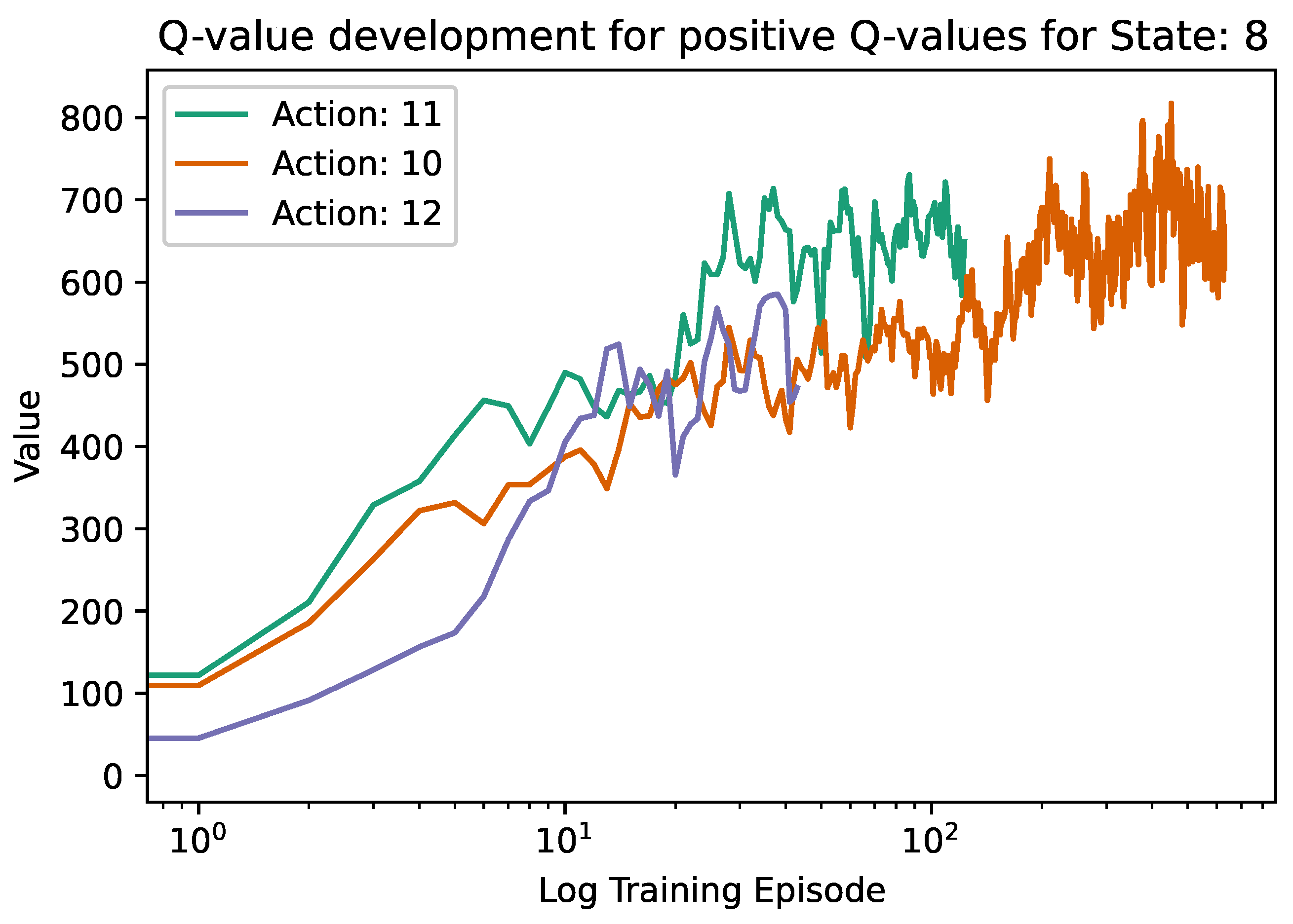
Figure 2. Schematic representation of crop rotation planning for a 5-year plan

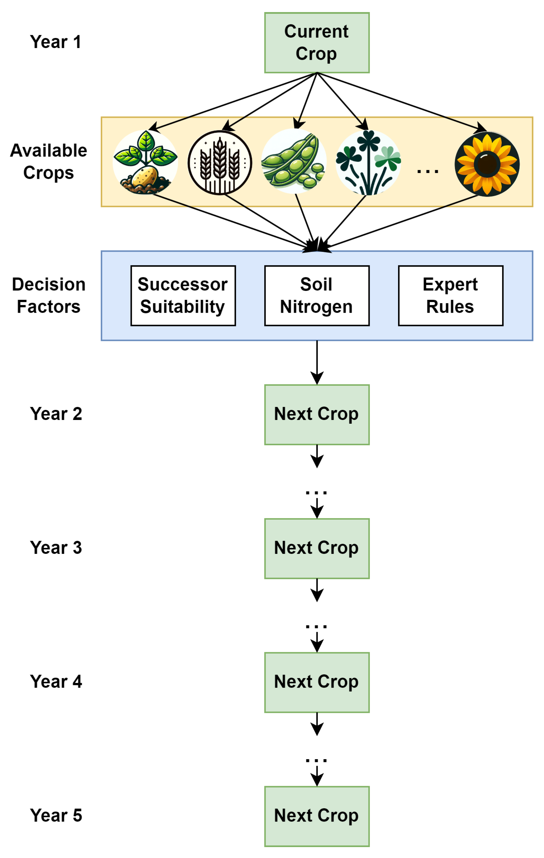
Figure 3. This figure depicts the pipelines we employed for designing crop rotations. From left to right: Crop yield information for 26 crops is used in the environment for both tabular reinforcement learning (RL) and deep reinforcement learning (DRL) agents. The agents train on these yields as deterministic rewards to derive crop rotation plans. For the perturbed yields, robustifications are applied to the tabular RL agents before all agents learn on the randomized rewards. Experts evaluate the resulting plans and the additional explanations obtained during the learning process.

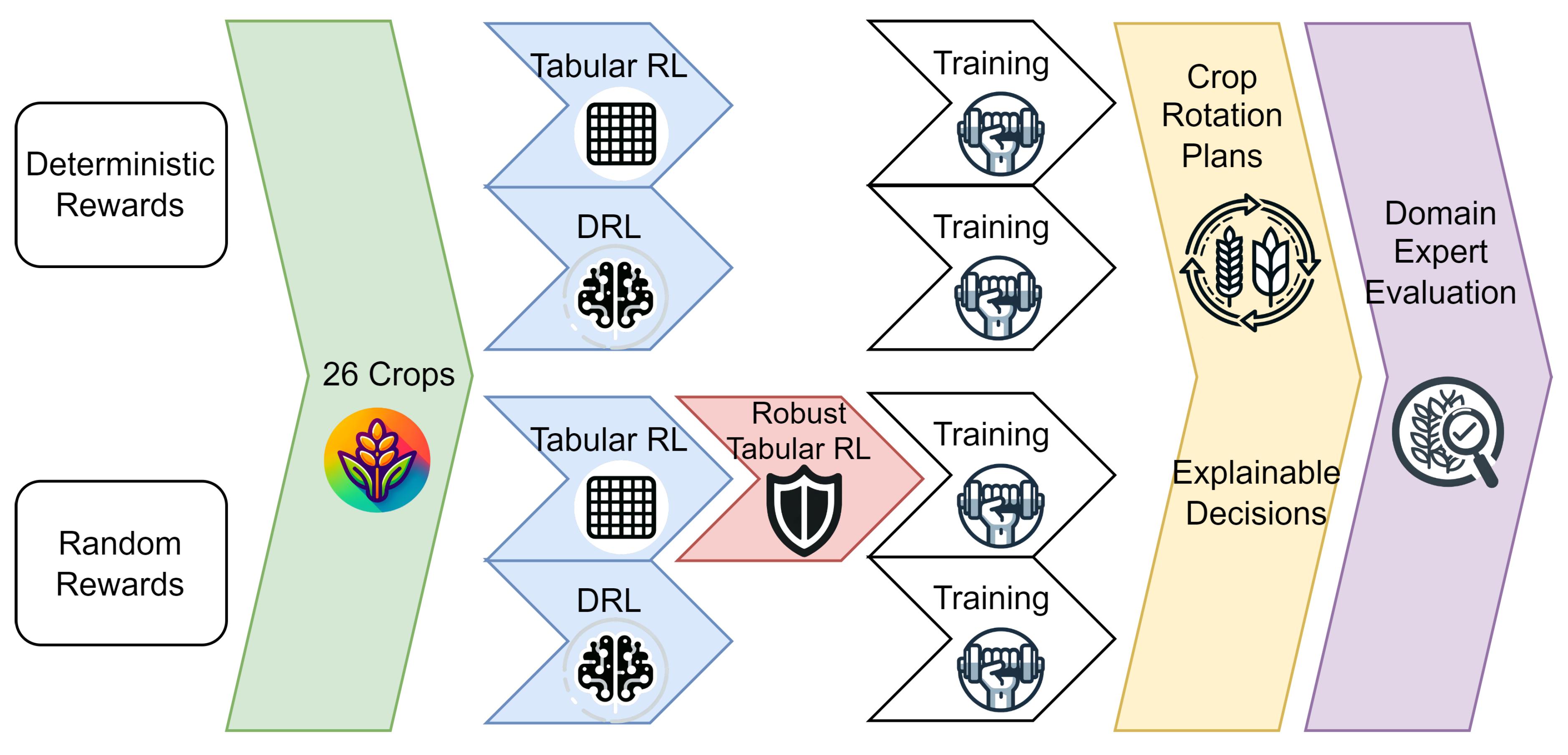
Figure 4. Comparison of average rewards development during training on non-random rewards for DQN and tabular agents

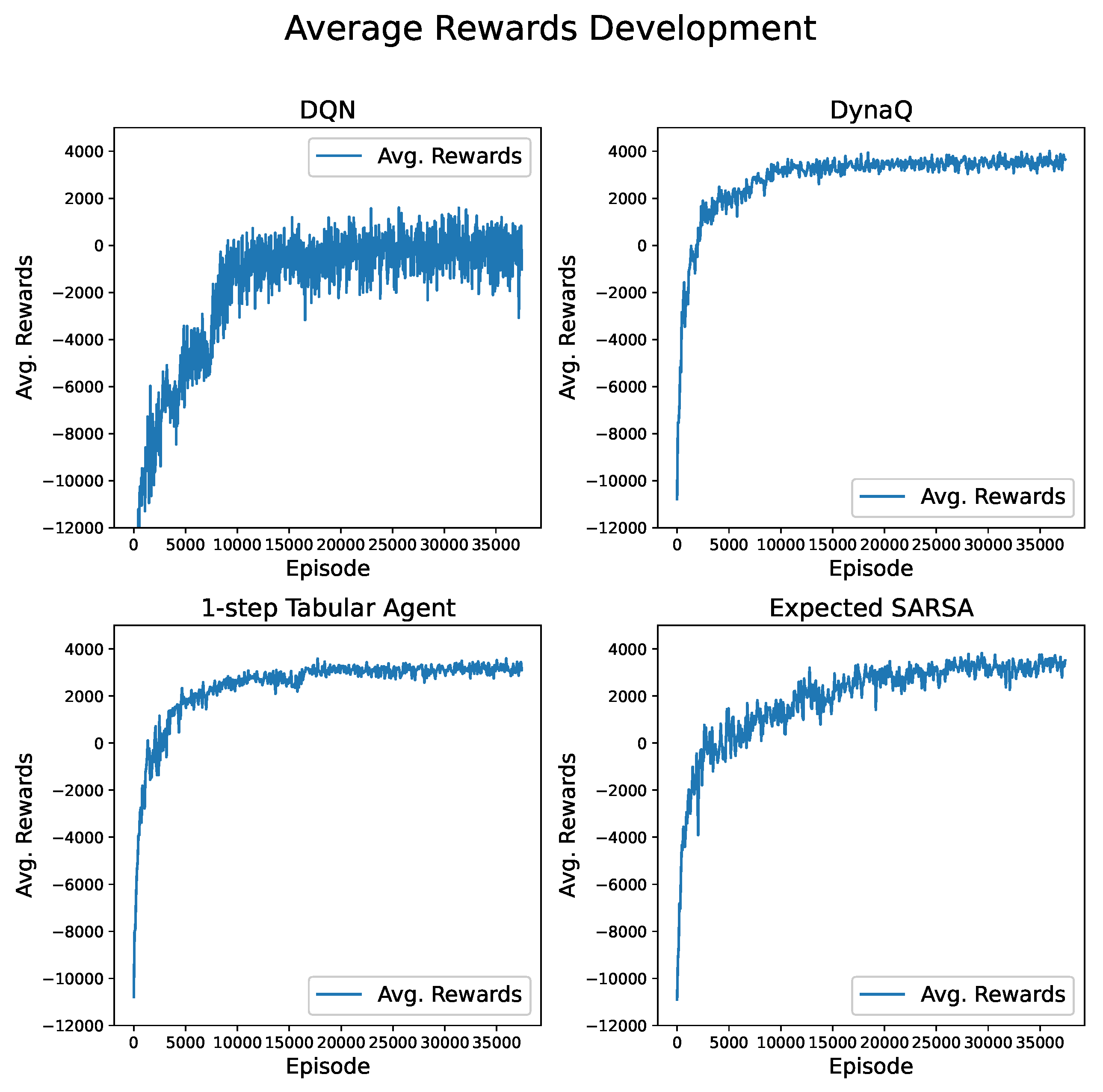
Figure 5. Non-chronological Q-value development during the training process for all potential actions in State 4

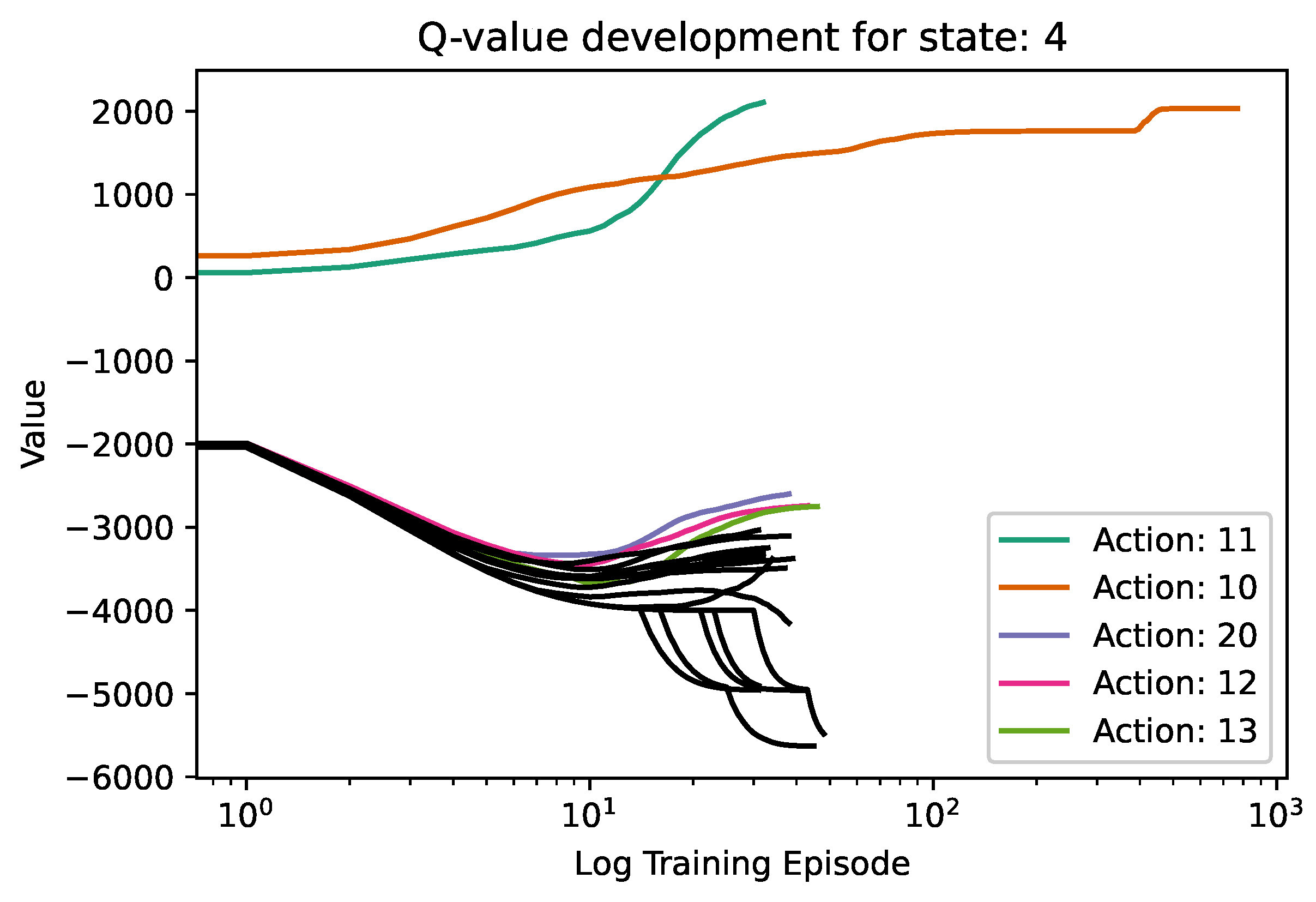
Figure 6. Chronological Development of the best Strategy for Starting Crop 4.

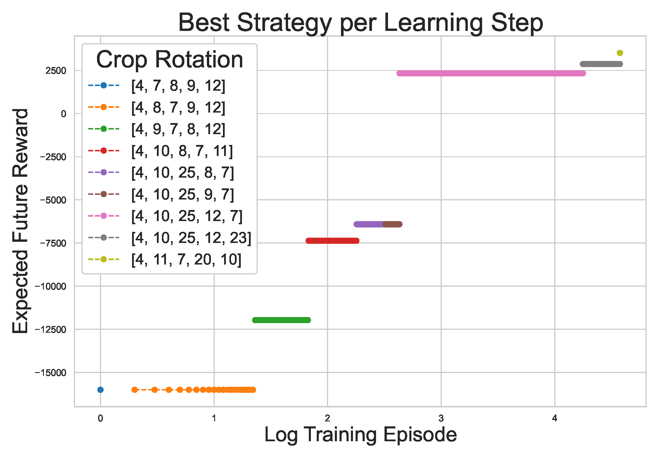
Figure 7. Soil nitrogen and yield development

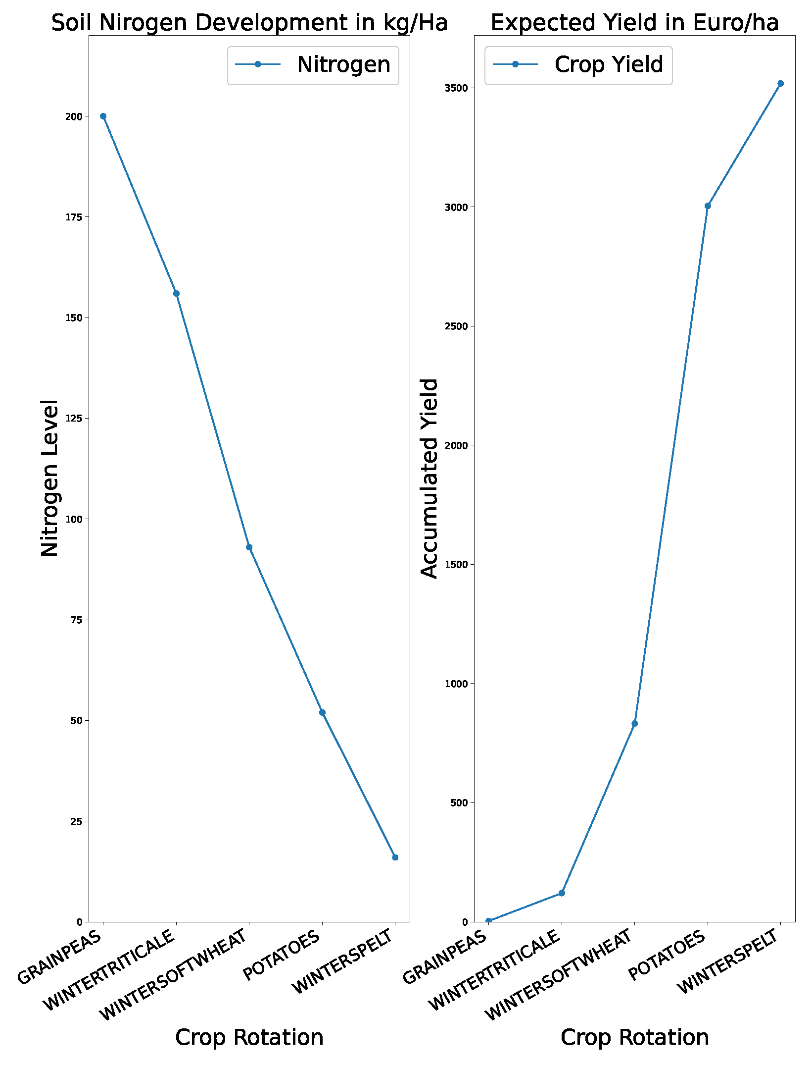
Figure 8. Explainability Tree that shows from top to bottom the suggested crop rotation. To the right of each suggestion, there are boxes that depict how many crops violated which rule and how many were unsuitable in the regard that they have lower yields.

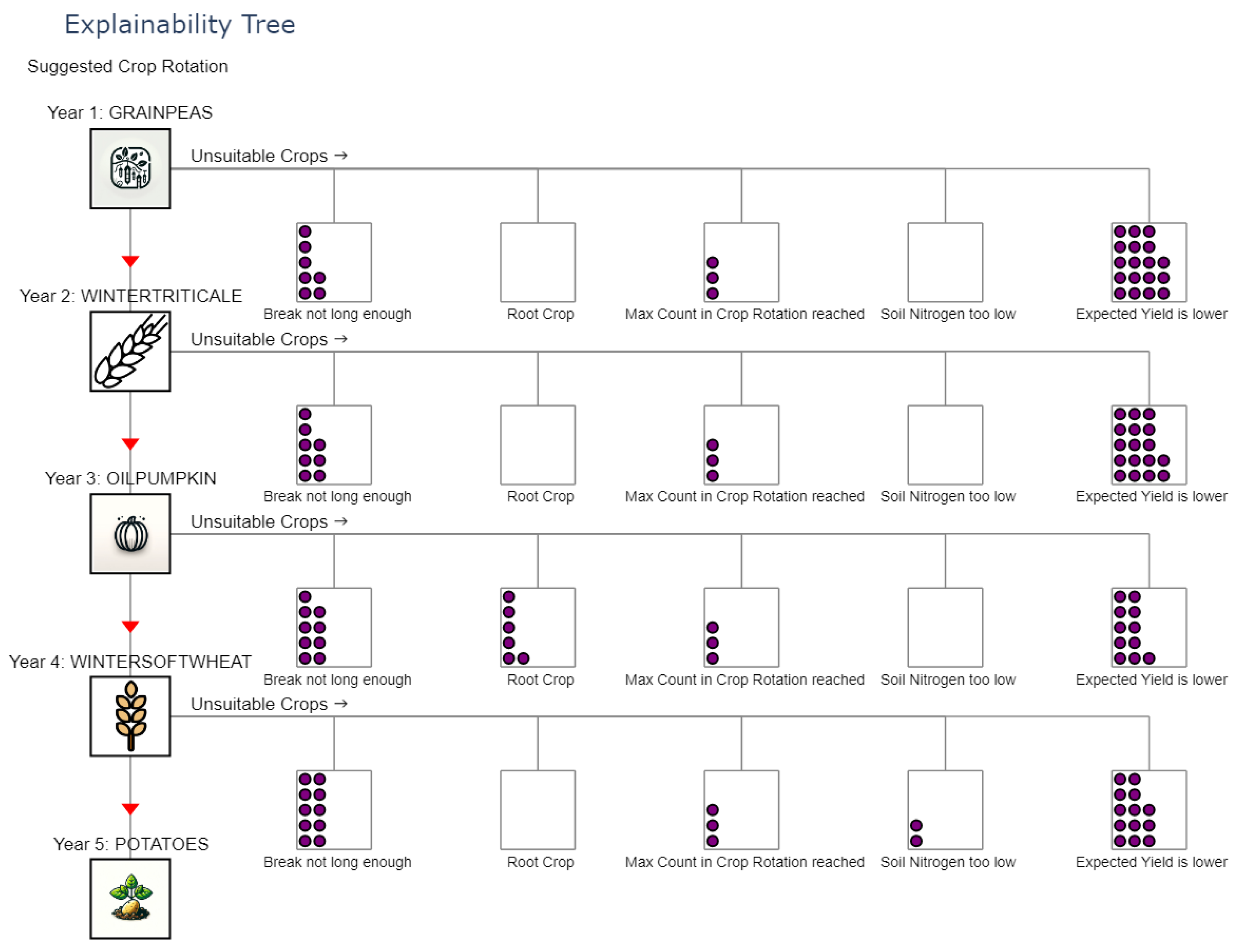
Figure 9. Comparison of average rewards development during training on random rewards for DQN and tabular agents

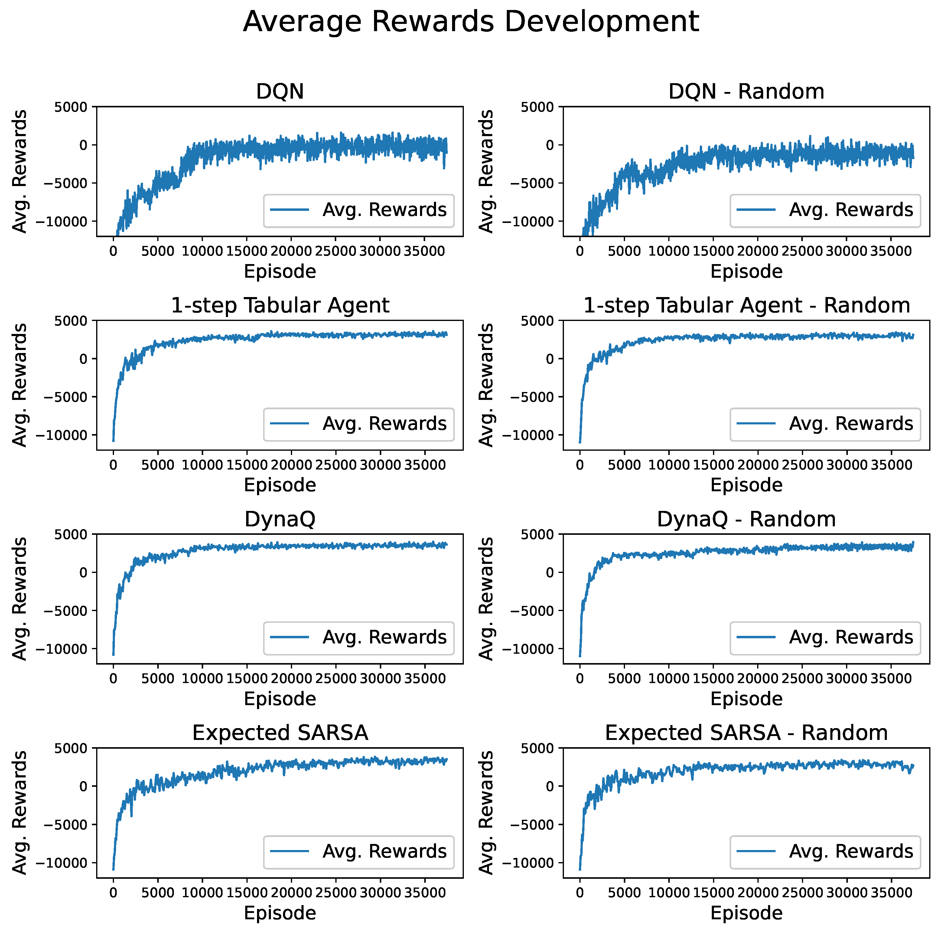
Figure 10. Chronological development of the best strategy for Starting Crop 8

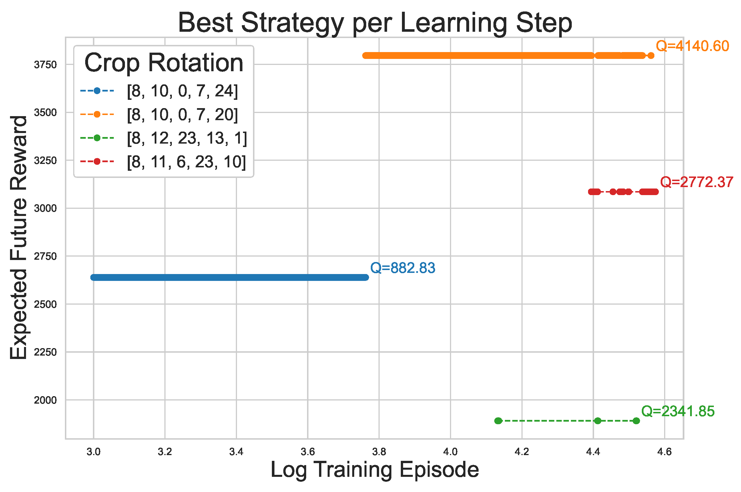
Figure 11. Comparison of average rewards during training for old and new argmax function for the DynaQ agent

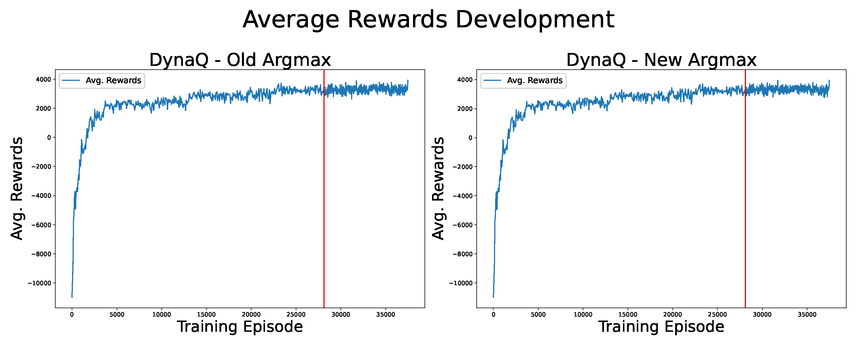
Figure 12. Q-value development comparison between old and new argmax function for 1 state-action pair

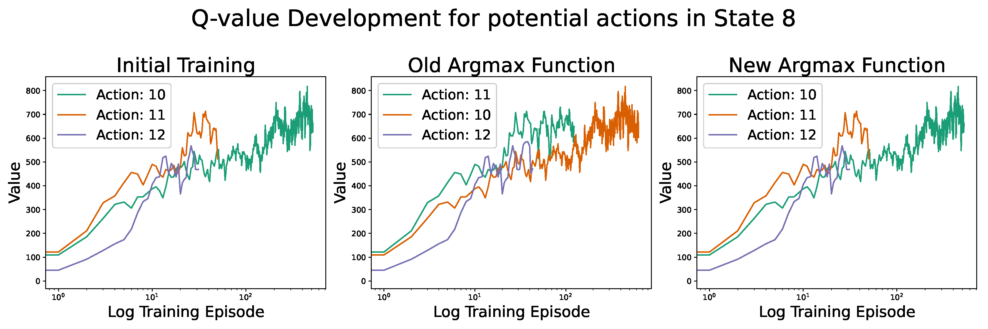
Figure 13. Chronological Development of the Best Strategy for Starting Crop 8 - Robust Learning

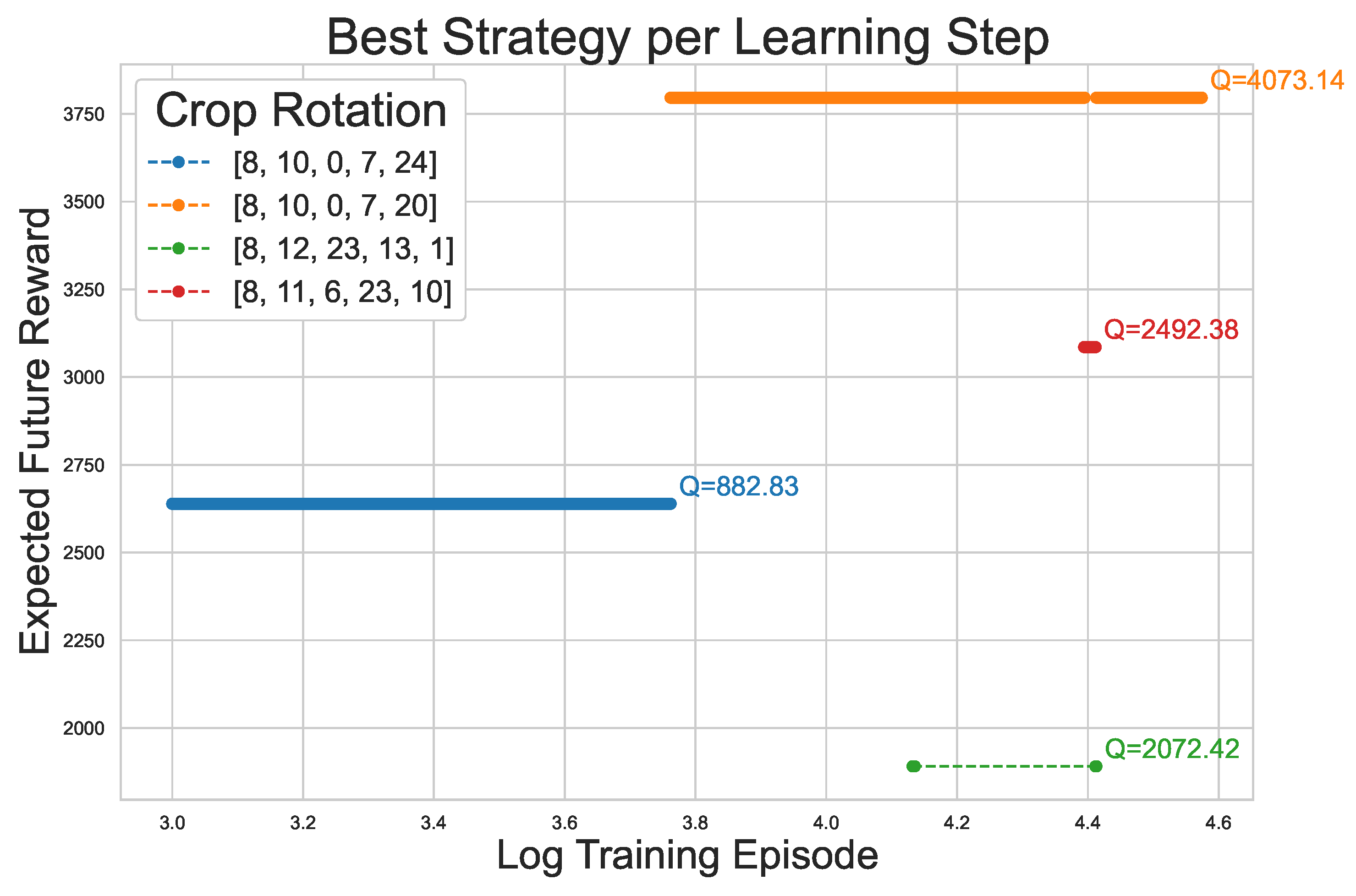
Table 1. Tabular RL categories.

	On-policy	Off-policy
Model based	Model-Based Policy Iteration; Monte Carlo Tree Search (MCTS)	DynaQ
Model free	SARSA (on-policy)	n-step Q-learning; Q-learning with function approx.

Table 2. Strategy Results Non-Random Rewards.

	DQN	1-Step Q-Learning	DynaQ	Expected SARSA
Number of best Strategies	1	7	15	18
Reward Best Strategy	3573 (12)	4759 (1)	5337 (4)	5447 (1)
Reward 2nd Best Strategy	3515 (3)	4645 (1)	4722 (2)	5337 (1)
Reward 3rd Best Strategy	-602 (2)	4604 (1)	4645 (1)	5140 (1)

Table 3. Strategy differences based on non-random or random Reward when taking each crop at the start of the crop rotation once.

	Non-Random Better	Equal	Random Better
1-step Q-learning	11	5	10
DynaQ	11	8	7
Expected SARSA	15	4	7

Table 4. Non-Random Rewards vs. Random Rewards

	Median Reward	Mean Reward	SD Reward
Regular Argmax	3286	3283	204
New Argmax	3316	3316	192

Table 5. Average Rewards over all final suggestions for each starting crop - non-random rewards vs. random rewards

	Non-Random Rewards	Random Rewards
1-step Q-learning	3188	3022
DynaQ (Ensemble)	3550	3740
Expected SARSA	3172	2473

Table 6. Strategy differences based on non-random or random Reward when taking each crop at the start of the crop rotation once - after robustification

	Non-Random Better	Equal	Random Better
1-step Q-learning	9	6	11
DynaQ (Ensemble)	5	10	11
Expected SARSA	16	6	4

Table 7. Crop Rotation Preference as answered by the domain experts

	Starting Crop	Preference
		Non-Random	Random	None
Non-random scores higher	Spring Barley	1	2
	Grain Maize	1	1	1
	Winter Rye	2	1
Random scores higher	Grain Peas	0	3
Random scores higher	Sommer Oat	0	2	1
Equal Score	Potatoe	-	-	-

Table 8. Risk evaluation as answered by the domain experts

	Starting Crop	Economical Risk
		Not Risky at All	Not Risky	Acceptable	Risky	Very Risky
Non-random scores higher	Spring Barley	-	1	2	-	-
	Grain Maize	1	1	-	-	1
	Winter Rye	-	1	2	-	-
Random scores higher	Grain Peas	-	1	2	-	-
Random scores higher	Sommer Oat	-	1	1	1	-
Equal Score	Potatoe	-	1	2	-	-

Disclaimer/Publisher’s Note: The statements, opinions and data contained in all publications are solely those of the individual author(s) and contributor(s) and not of MDPI and/or the editor(s). MDPI and/or the editor(s) disclaim responsibility for any injury to people or property resulting from any ideas, methods, instructions or products referred to in the content.

© 2024 by the authors. Licensee MDPI, Basel, Switzerland. This article is an open access article distributed under the terms and conditions of the Creative Commons Attribution (CC BY) license (http://creativecommons.org/licenses/by/4.0/).

Copyright: This open access article is published under a Creative Commons CC BY 4.0 license, which permit the free download, distribution, and reuse, provided that the author and preprint are cited in any reuse.

Downloads

Views

Comments

Subscription

Notify me about updates to this article or when a peer-reviewed version is published.

MDPI Initiatives

Important Links

Choose an area of interest and we will send you notifications of new preprints at your preferred frequency.

Disclaimer

Tabular Reinforcement Learning for Reward Robust, Explainable Crop Rotation Policies Matching Deep Reinforcement Learning Performance

Abstract

Keywords:

Subject:

1. Introduction

2. State of the Art & Related Work

3. Methodology

3.1. Definitions

3.2. Reinforcement Learning Methods

3.3. Tabular Reinforcement Learning Methods

3.4. Markov Property

3.5. Robustifying Tabular Algorithms

3.6. Robust Planning

3.7. Deep Reinforcement Learning Method

3.8. Setting the Random Rewards

4. Experimental Design and Setup

5. Results

5.1. DRL vs. Tabular RL: Non-Random Rewards

5.1.1. Overall Rewards During Training

5.1.2. Explainability for non-Random Rewards

5.2. DRL vs. Tabular RL: Random Rewards

5.3. Overall Rewards During Training

5.3.1. Update Argmax for Exploration

5.3.2. Differing Planning Strategies for DynaQ

5.4. Robust Random Reward learning vs. non-Random Reward Learning

5.4.1. Summary

5.5. Domain Expert Evaluation

6. Discussion

7. Conclusion & Future Research

Acknowledgments

Appendix A

References

MDPI Initiatives

Important Links

Subscribe