Neural Network-Based Parameter Estimation in Dynamical Systems

Dimitris Kastoris; Kostas Giotopoulos; Dimitris Papadopoulos

doi:10.20944/preprints202411.0076.v1

Preprint

Article

Neural Network-Based Parameter Estimation in Dynamical Systems

This version is not peer-reviewed.

Dimitris Kastoris,

Kostas Giotopoulos

Dimitris Papadopoulos^*

Dimitris Kastoris,

Kostas Giotopoulos

Dimitris Papadopoulos^*

This version is not peer-reviewed.

Downloads

Views

Comments

Submitted:

01 November 2024

Posted:

01 November 2024

You are already at the latest version

A peer-reviewed article of this preprint also exists.

Abstract

Mathematical models are designed to assist decision-making processes across various scientific fields. These models typically contain numerous parameters, the values’ estimation of which often comes under analysis when evaluating the strength of these models as management tools. Advanced artificial intelligence software, has proven to be highly effective in estimating these parameters. In this research work, we use the Lotka-Volterra model to describe the dynamics of a telecommunication sector in Greece and then we propose a methodology that employs a feed-forward neural network (NN). The NN is used to estimate the parameter’s values of the Lotka-Volterra system, which are later applied to solve the system using a fourth algebraic order Runge-Kutta method. The application of the proposed architecture to the specific case study, reveals that the model fits well to the experiential data. Furthermore, the results of our method surpassed the other three methods used for comparison, demonstrating its higher accuracy and effectiveness. The implementation of the proposed feed-forward neural network as well as the fourth algebraic order Runge-Kutta method was accomplished using MATLAB.

Keywords:

Lotka-Volterra

;

feed-forward neural network

;

MATLAB

;

Runge-Kutta method

Subject:

Computer Science and Mathematics - Artificial Intelligence and Machine Learning

1. Introduction

The primary purpose of mathematical modeling is to simplify and explain complex systems that occur in many scientific fields. Our goal is to develop a straightforward model that precisely fits a data set within a defined margin of error, while also enabling the exploration of specific properties. Our research utilizes a feed-forward neural network to estimate the parameters’ values of the Lotka-Volterra model. Neural networks (NNs) have emerged as a adjustable tool for solving complex systems, especially when integrated with experimental data [1]. By training a neural network on such data, the model can reveal hidden patterns and complex relationships that are difficult to capture through traditional approaches. NNs are particularly effective in controlling noisy, non-linear, or high-dimensional datasets, which improve their ability to estimate parameters and make accurate predictions [2]. When used to experimental datasets, neural networks prove strong generalization capabilities, providing valuable information into system dynamics and enabling the construction of accurate models for a variety of scientific applications [3]. In the case of a Lotka-Volterra system, the parameter values typically represent factors such as competition, mutualism, predation, or growth between interacting species/populations. These parameters must be quantified to effectively apply the model as a decision making tool in a specific context [4]. The challenge, is to accurately quantify these parameters to solve the problem quantitatively and ensure the model closely fits the raw data. In the literature there are several techniques which are trying to achieve this target. For instance, Shatalov et al. [5] and Fedatov and Shatalov [6] propose a method that involves using direct integration to acquire goal functions and applying subsequent quadrature rules to determine the values of the unknown parameters. On the other hand, Michalakelis et al. [7] employ genetic algorithms techniques and advanced computer software to solve a non-linear system.

To demonstrate the practical application of the proposed method (FFNN2HL), we use a Lotka-Volterra system that describes the dynamics among three competitors in the telecommunication market, relying on a comprehensive set of data. The problem is constructed as a dynamical system containing of three nonlinear first-order differential equations, each including both linear and quadratic terms, comparable to the systems discussed by Bazykin [8] and Fay and Greeff [9]. Market concentration has long been a focus of researchers, particularly concerning the number of firms offering specific products or a range of products and services [10]. The structure of a market is crucial in determining market power, business behavior, and overall performance, which in turn facilitates the assessment of the level of competition across different industries. These considerations are especially relevant in the high-technology sector, such as telecommunications. Traditionally, telecommunications were operated as a national monopoly until recent years when market liberalization occurred. This change transformed the market from a monopolistic structure, characterized by important entry barriers, to an oligopolistic or, in some cases, a competitive environment. Therefore, the analysis of this emerged market is basic for identifying its unique characteristics, understanding competitor behaviors, and providing valuable insights for lawmaking and regulatory authorities [10,11].

The proposed neural network architecture is based on a feed-forward neural network with one input layer, two hidden layers and an output layer consists of three nodes. In this structure, the input vector is processed through the hidden layers, where non-linear transformations are applied, allowing the network to model complex patterns of the experimental data. The three output nodes, serve the prediction of multiple target variables simultaneously, making the neural network ideal for tasks that include multiple outputs. This architecture enables the model to operate in a data-driven learning mode, producing reliable predictions.

2. Overview of the Lotka–Volterra Model Interpretation

The well-known Lotka–Volterra (LV) model is often utilized in order to represent the dynamics of n interacting species within an ecosystem. The LV model is represented by the following system of ordinary differential equations (ODEs):

\frac{d x_{i}}{d t} = x_{i} (a_{i 0} + \sum_{j} a_{i j} x_{j}), i, j = 1, 2, \dots, n,

(1)

where

\frac{d x_{i}}{d t}

represents the rate of change in the population size of each of the n species. The parameters

a_{i 0}

describe either the intrinsic population growth or decline of species i in the lack of interactions with other species (positive values indicate growth while negative values indicate decline). Furthermore, the parameters

a_{i j}

can be positive, negative, or zero, reflecting whether the species interact through predation, rivalry, mutualism, or have no interaction at all. For n interacting species the general Lotka–Volterra system of Eq. 1 takes the following form:

\begin{matrix} \frac{d x}{d t} = x (a_{10} + a_{11} x + a_{12} y + a_{13} z) \\ \frac{d y}{d t} = y (a_{20} + a_{21} x + a_{22} y + a_{23} z) \\ \frac{d z}{d t} = z (a_{30} + a_{31} x + a_{32} y + a_{33} z) \end{matrix}

(2)

where x, y, z are the three competitors.

3. Description of the Method

In this section, we present the proposed methodology for estimating parameter’s value in dynamic systems which are defined by nonlinear ODEs. The method applies a feed-forward neural network and uses optimization techniques for the determination of the values. The effectiveness of the proposed approach is demonstrated on a Lotka-Volterra system with three interacting competitors, where time-series data is available for each. The numerical results emphasize the efficacy of the method in capturing the system’s dynamics.

Valid parameter estimation in dynamic systems is crucial across many scientific and engineering disciplines. Traditional approaches often involve linearization or demand wide prior knowledge of the system’s structure, which can be difficult when dealing with nonlinearities and intricate variable interactions. In this study, we present a method that uses the capabilities of neural networks to model complex relationships, coupled with optimization techniques to estimate the parameters of a nonlinear dynamic system.

3.1. Data Collection and Normalization

In our application we use time-series data for the three variables in the system (2), which were collected over a time span of 19 six-monthly periods. Data for variables

x (t)

y (t)

and

z (t)

were stored in the vectors

x_{data}

y_{data}

, and

z_{data}

, respectively. For more effective and efficient network training, we normalize the data by subtracting the mean and dividing by the standard deviation of each variable.

3.2. Neural Network Architecture:

A feed-forward neural network was designed with the following architecture:

Input Layer: A single feature input representing time ( $t_{data}$ ).
Two Fully Connected Hidden Layers: Each with n possible neurons and a hyperbolic tangent activation function (tanh). Custom weight and bias initializers were used to ensure small initial weights and zero biases.
Output Layer: A fully connected layer producing three outputs, corresponding to the predictions of $x (t)$ , $y (t)$ , and $z (t)$ . Regression layer in each output is used to calculate the loss based on the difference between the predicted and normalized true values.

In this case, the neural network (NN) plays the role of modeling the time evolution of the system represented by three variables (

x_{d a t a}

y_{d a t a}

, and

z_{d a t a}

) based on time (t).

Basic Roles:

1. Prediction of system dynamics: The NN is trained on normalized data (

x_{data}

y_{data}

z_{data}

) to predict the values of x, y, and z over time (t). After training, it can generate predictions (YPred) for the system based on the time data.

2. Learning the relationships: The NN is developed to approximate the underlying dynamics between the variables (x, y, z) and time (t), allowing the model to capture the relationships between these variables that might be nonlinear or complex.

3. Providing inputs for further analysis: The NN’s predictions are denormalized to provide continuous estimates of the system variables, which are then used to compute the derivatives (

\frac{d x}{d t}

\frac{d y}{d t}

\frac{d z}{d t}

). These derivatives are essential for parameter estimation using fminunc in the subsequent optimization process.

In summary, the NN approximates the time-dependent behavior of the system variables and provides predictions that are crucial for calculating the derivatives needed for optimization.

3.2.1. Feed-Forward Propagation

A feed-forward neural network operates according to following procedure [29]: for each data point

t^{(i)}

, the learning process begins by setting

a_{1}^{[0]} = t^{(i)}

. Next, to compute

a^{l}

from

a^{l - 1}

, we follow two key steps. The first step involves calculating an intermediate vector

z^{l}

by performing a matrix multiplication between the previous layer’s activations

a^{l - 1}

and the weight matrix

W^{l}

, and then adding the bias vector

b^{l}

. This can be represented as:

z_{j}^{l} \equiv \sum_{k = 1}^{h^{l - 1}} W_{j k}^{l} a_{k}^{l - 1} + b_{j}^{l} .,

(3)

Alternatively, in matrix notation, Equation (3) becomes:

z^{l} = W^{l} a^{l - 1} + b^{l} .

(4)

The next step involves the application of an activation function

σ^{l}

to the values in

z^{l}

to produce the activations

a^{l}

from (4). This step can be expressed as:

a^{l} = σ^{l} (z^{l}) = σ^{l} (W^{l} a^{l - 1} + b^{l}) .

(5)

In summary, for each input data point

t^{(i)}

, we compute both

z^{l}

and the output

a^{l}

by using Equations (4) and (5) respectively. To emphasize the dependence on the input

t^{(i)}

, we can denote the activations and intermediate values as

a^{l (i)} = σ^{l} (z^{l (i)})

. Thus, using matrix and vector notation, we can summarize the forward pass across all data points as follows:

\begin{matrix} T & = & [t_{1}, \dots, t_{N}], \\ Z^{l} & = & [z^{l (1)}, \dots, z^{l (N)}], \\ A^{l} & = & [a^{l (1)}, \dots, a^{l (N)}] . \end{matrix}

(6)

Using the notation of (6) we lead to the recursive update rules:

\begin{matrix} A^{0} & = & T, \\ Z^{l} & = & W^{l} A^{l - 1} + b^{l}, \\ A^{l} & = & σ^{l} (Z^{l}), for l = 1, \dots, L . \end{matrix}

(7)

The output layer

A^{L}

represents the final output of the network, denoted as:

N (T, W^{L}, b^{L}) = A^{L} .

(8)

Alternatively, in component form, we write the network output as:

N_{j} (t^{(i)}, W^{L}, b^{L}) = π_{j} (A^{L}) = A_{j}^{L} (t^{(i)}, W, b),

(9)

where

π_{j}

in (9) refers to the j-th component of the output vector.

3.3. Training Process,Prediction and Denormalization

The neural network was trained utilizing the Adam optimization algorithm, running for a total of 20,000 epochs. The initial learning rate was set to 0.01. A batch size of 19 was used, meaning the entire dataset was processed in each iteration without shuffling the data between epochs, in order to maintain the temporal sequence of the data.To track the training process and ensure convergence, a live plot displaying training progress was employed. Upon completing the training, the network was applied to predict the normalized values of

x (t)

y (t)

, and

z (t)

for the entire time series. These predicted values were subsequently denormalized using the original mean and standard deviation of the dataset.

3.3.1. Back Propagation

Backpropagation is an algorithm used for training feed-forward neural networks [21]. It involves two main phases:

1. Forward Pass: The input data is passed through the network, and the output is calculated.

2. Backward Pass (Backpropagation): The error (difference between the predicted output and actual output) is propagated backward through the network. The gradients of the loss function with respect to each weight are calculated, and the weights are updated using these gradients (often via a gradient-based optimization method like Adam or SGD).

Backpropagation relies on the chain rule of calculus to compute the derivatives of the loss function with respect to the weights.

Here’s the general mathematical form:

Given

a^{L}

is the output of the network at the final layer L (predicted output),

y

is a true label or ground truth, C is the cost function or loss function (e.g., Mean Squared Error or Cross-Entropy Loss),

W^{l}

and

b^{l}

are the weights and biases of layer l,

a^{l}

the activation at layer l,

z^{l}

the weighted input at layer l, where

z^{l} = W^{l} a^{l - 1} + b^{l}

and

σ

is the activation function (e.g., Sigmoid, ReLU, Tanh).

1.Loss (Cost) Function:

The loss function C measures the error between the predicted output

a^{L}

and the true output

y

. For a given training example, it can be represented as:

C = \frac{1}{2} \sum {(a^{L} - y)}^{2}

(10)

This is just one example (for Mean Squared Error), but the form of C will vary depending on the task and choice of loss function.

2.Gradients in the Output Layer (Layer L):

The error at the output layer is defined as:

δ^{L} = \nabla_{a} C \circ σ^{'} (z^{L})

(11)

where

\nabla_{a} C = (a^{L} - y)

in (11) is the derivative of the loss function (10) with respect to the output activations, ∘ denotes element-wise multiplication (Hadamard product) and

σ^{'} (z^{L})

is the derivative of the activation function at the final layer.

3. Gradients in the Hidden Layers (Layer l):

For the hidden layers, the error is propagated backward using:

δ^{l} = {(W^{l + 1})}^{T} δ^{l + 1} \circ σ^{'} (z^{l})

(12)

where

{(W^{l + 1})}^{T}

is the transpose of the weight matrix from layer

l + 1

δ^{l + 1}

is the error from the next layer and

σ^{'} (z^{l})

is the derivative of the activation function for layer l.

4.Gradients with Respect to Weights and Biases:

Once the errors

δ^{l}

in (12) are calculated for each layer, the gradients of the loss with respect to the weights and biases are computed as:

\begin{matrix} \frac{\partial C}{\partial W^{l}} = δ^{l} {(a^{l - 1})}^{T}, \\ \frac{\partial C}{\partial b^{l}} = δ^{l} . \end{matrix}

(13)

5. Weight and Bias Updates (with learning rate $η$ ):

\begin{matrix} W^{l} = W^{l} - η \frac{\partial C}{\partial W^{l}}, \\ b^{l} = b^{l} - η \frac{\partial C}{\partial b^{l}} . \end{matrix}

(14)

3.3.2. Adam Optimizer

Based on the optimal learning parameters

W^{*}

and

b^{*}

from (13) and (14), we obtain the approximate solutions of the dynamical system. In our study, the Adaptive Moment Estimation (Adam) algorithm was employed to update these parameters. The update process follows the rules:

\begin{matrix} M_{w}^{k} & = & β_{1} M_{w}^{k - 1} + (1 - β_{1}) \nabla J_{1} (W^{k}), \\ M_{b}^{k} & = & β_{1} M_{b}^{k - 1} + (1 - β_{1}) \nabla J_{1} (b^{k}), \\ V_{w}^{k} & = & β_{2} V_{w}^{k - 1} + (1 - β_{2}) {(\nabla J_{1} (W^{k}))}^{2}, \\ V_{b}^{k} & = & β_{2} V_{b}^{k - 1} + (1 - β_{2}) {(\nabla J_{1} (b^{k}))}^{2}, \end{matrix}

(15)

where

β_{1}

and

β_{2} \in [0, 1)

are the decay rates for the moment estimates. The corrected moment estimates for the weights and biases are then given by:

\begin{matrix} {\hat{M}}_{w}^{k} = \frac{M_{w}^{k}}{1 - β_{1}^{k}}, {\hat{V}}_{w}^{k} = \frac{V_{w}^{k}}{1 - β_{2}^{k}}, \\ {\hat{M}}_{b}^{k} = \frac{M_{b}^{k}}{1 - β_{1}^{k}}, {\hat{V}}_{b}^{k} = \frac{V_{b}^{k}}{1 - β_{2}^{k}} . \end{matrix}

(16)

Finally, the weights and biases are updated as follows:

\begin{matrix} W^{k + 1} = W^{k} - η \frac{{\hat{M}}_{w}^{k}}{\sqrt{{\hat{V}}_{w}^{k}} + ϵ}, \\ b^{k + 1} = b^{k} - η \frac{{\hat{M}}_{b}^{k}}{\sqrt{{\hat{V}}_{b}^{k}} + ϵ} . \end{matrix}

(17)

In Equation 17,

η

is the learning rate,

ϵ

is a small constant to prevent division by zero, and

M_{w}

M_{b}

V_{w}

, and

V_{b}

are the first and second moment vectors initialized to zero. Commonly used values for the hyperparameters include

η = 0.001

β_{1} = 0.9

β_{2} = 0.999

, and

ϵ = 10^{- 8}

, as suggested by the literature [12].

3.4. Prediction Process After Training

Once the neural network has been trained, we use the time data as the input. This input is a one-dimensional array where each value corresponds to a specific time point, representing the system’s behavior at that instant. Essentially, the input is a sequence of time points that the network encountered during training. The trained neural network is then employed to predict the normalized output values for the variables

x (t)

y (t)

, and

z (t)

over the entire time series. In MATLAB, this is achieved by using the predict function with the time data as input. The network processes each time step individually and produces a corresponding set of three outputs, one for each variable (x, y, and z). Since the network’s predictions are in their normalized form (because the training data was normalized before input), we must convert them back to their original scale. This is done by reversing the normalization, applying the mean and standard deviation that were initially used to normalize the data. The final output is a matrix, where each row corresponds to a specific time point and the columns represent the denormalized predictions for

x (t)

y (t)

, and

z (t)

at that point in time. These predictions can be directly compared to the actual measured values or used for further computations, such as determining derivatives to estimate system parameters.

3.5. Parameter Estimation via Optimization

The predicted values were utilized to calculate the numerical derivatives with respect to time, applying finite difference methods. These derivatives were then related to the parameters of the dynamic system through a set of nonlinear equations. The general form of these equations is as follows:

\begin{matrix} \frac{d x}{d t} = x (t) \cdot (a_{10} + a_{11} \cdot x (t) + a_{12} \cdot y (t) + a_{13} \cdot z (t)) \\ \frac{d y}{d t} = y (t) \cdot (a_{20} + a_{21} \cdot x (t) + a_{22} \cdot y (t) + a_{23} \cdot z (t)) \\ \frac{d z}{d t} = z (t) \cdot (a_{30} + a_{31} \cdot x (t) + a_{32} \cdot y (t) + a_{33} \cdot z (t)) \end{matrix}

(18)

In the Eq.19 , the time derivatives of

x (t)

y (t)

, and

z (t)

are expressed in terms of the unknown parameters

a_{10}

through

a_{33}

, and the values of the variables at each time step.

The parameters

a_{10}

a_{33}

were determined by minimizing the sum of the squared differences between the left-hand and right-hand sides of the system of equations. This minimization was carried out using the quasi-Newton optimization technique, specifically the fminunc function in MATLAB. The mathematical formulation for minimizing the sum of squared differences between the left-hand and right-hand sides of the system of Eq.18 can be expressed as:

\begin{matrix} minimize \sum_{i = 1}^{N} {(\frac{d x (t_{i})}{d t} - x (t_{i}) \cdot (a_{10} + a_{11} \cdot x (t_{i}) + a_{12} \cdot y (t_{i}) + a_{13} \cdot z (t_{i})))}^{2} \\ + \sum_{i = 1}^{N} {(\frac{d y (t_{i})}{d t} - y (t_{i}) \cdot (a_{20} + a_{21} \cdot x (t_{i}) + a_{22} \cdot y (t_{i}) + a_{23} \cdot z (t_{i})))}^{2} \\ + \sum_{i = 1}^{N} {(\frac{d z (t_{i})}{d t} - z (t_{i}) \cdot (a_{30} + a_{31} \cdot x (t_{i}) + a_{32} \cdot y (t_{i}) + a_{33} \cdot z (t_{i})))}^{2} \end{matrix}

(19)

where:

N is the number of time points,
$t_{i}$ represents each time point,
$\frac{d x (t_{i})}{d t}, \frac{d y (t_{i})}{d t}, \frac{d z (t_{i})}{d t}$ are the time derivatives of the variables $x, y, z$ ,
$a_{10}, a_{11}, \dots, a_{33}$ are the parameters to be estimated.

3.5.1. Mathematical Formulation of Quasi-Newton Method

The quasi-Newton optimization method is a numerical approach designed for minimizing functions, particularly those that are not necessarily quadratic. It simulates the behavior of Newton’s method but circumvents the direct computation of the Hessian matrix by iteratively refining an estimate of it. MATLAB’s fminunc function typically utilizes the Broyden–Fletcher–Goldfarb–Shanno (BFGS) algorithm [13], or its limited-memory version (L-BFGS), to perform the optimization.

Let

f (p)

be the function to be minimized, where

p

is a vector of parameters. The iterative update of the parameter vector

p

at the k-th step is given by:

p_{k + 1} = p_{k} - α_{k} B_{k}^{- 1} \nabla f (p_{k})

(20)

where:

$p_{k}$ is the parameter vector at iteration k,
$α_{k}$ is the step size (also known as the learning rate),
$B_{k}^{- 1}$ is an approximation of the inverse Hessian matrix,
$\nabla f (p_{k})$ is the gradient of the function $f (p)$ evaluated at $p_{k}$ .

In quasi-Newton methods, instead of calculating the Hessian matrix

H_{k}

directly, the inverse Hessian approximation

B_{k}^{- 1}

is updated iteratively using information from the gradient. This update typically follows the BFGS algorithm:

B_{k + 1} = B_{k} + Δ B_{k}

(21)

In Equation (21),

Δ B_{k}

represents the update to the inverse Hessian matrix, derived from differences between consecutive gradients and parameter values. In essence, the quasi-Newton method employed by fminunc works by iteratively adjusting the parameter vector

p

in 20 based on estimates of the inverse Hessian matrix and gradient information. This approach helps efficiently locate the minimum of the objective function without the computational cost of directly calculating second-order derivatives.

3.6. Solving the System with Runge-Kutta method

After estimating the parameters, they were incorporated back into the Lotka-Volterra system of differential equations to simulate the system’s dynamics. To solve these equations, we used the Runge-Kutta 4th order method [22], a robust and accurate numerical method for solving ordinary differential equations. This method was applied over the same time interval as the original dataset. For solving first-order ordinary differential equations (ODEs), we utilize the Runge-Kutta method, which is known for its accuracy and efficiency [14,22,27]. However, when dealing with second-order ODEs, the Runge-Kutta-Nyström [23,24,25,26,28] method is preferred as it is specifically designed to handle second-order systems directly, offering improved performance by leveraging the structure of the equations [24].

The solutions obtained from this method were then compared with the experimental data. This comparison was used to assess how well the estimated parameters fit the system’s behavior, providing insight into the accuracy of the model. A visual comparison between the simulated trajectories and the data allowed us to evaluate the fit, and error metrics were calculated to quantify the accuracy.

3.6.1. Mathematical Formulation of the Runge-Kutta Method

The Runge-Kutta methods are used for the numerical solution of a first-order ordinary differential equation (ODE) of the form

\frac{d y}{d t} = f (t, y), y (t_{0}) = y_{0}

(22)

The Runge-Kutta method approximates the solution of (22) by using the following iterative scheme:

\begin{matrix} y_{n + 1} & = & y_{n} + h \sum_{i = 1}^{s} b_{i} k_{i}, \\ k_{i} & = & f (t_{n} + c_{i} h, y_{n} + h \sum_{j = 1}^{i - 1} a_{i j} k_{j}), for i = 1, 2, \dots, s . \end{matrix}

(23)

where

h is the step size,
s is the number of stages in the method and
$k_{i}$ are the stages of the method.
$a_{i j}, b_{i},$ and $c_{i}$ are the coefficients that define a specific Runge-Kutta method.

From the general form of Runge-Kutta methods (23) we can derive the desired algebraic order scheme. The Runge-Kutta method that we use in this case is a fourth algebraic order Runge-Kutta method of four stages [22].

Given the initial condition

y (t_{0}) = y_{0}

, the value of y at the next time step

t_{n + 1} = t_{n} + h

is computed as:

\begin{matrix} y_{n + 1} & = & y_{n} + \frac{h}{6} (k_{1} + 2 k_{2} + 2 k_{3} + k_{4}), \\ k_{1} & = & f (t_{n}, y_{n}), \\ k_{2} & = & f (t_{n} + \frac{h}{2}, y_{n} + \frac{h}{2} k_{1}), \\ k_{3} & = & f (t_{n} + \frac{h}{2}, y_{n} + \frac{h}{2} k_{2}), \\ k_{4} & = & f (t_{n} + h, y_{n} + h k_{3}) . \end{matrix}

(24)

This iterative process is repeated for each step, producing an approximation to the solution of the differential equation of the general form (22).

4. Example

4.1. Case Study Description

In system analysis, one common challenge is the lack of accessible and reliable datasets. However, a comprehensive historical dataset for three competitors in the Greek mobile telecommunications market was published by Michalakelis et al [7]. In their work, they proposed a Lotka-Volterra model of competing species to explain the dynamics between these companies. The goal of their research was to predict the potential of maintaining a steady and strong competitive equilibrium in the market, using the available data to analyze market share control in the mobile phone industry over some specific years.

The study examines the historical market penetration and future prospects of the three competing service providers. The dataset covers the years 1995 to 2007, but since the second competitor, y, only entered the market in 1998, the analysis of the three competitors begins with the initial conditions from 1998. Each data point reflects the percentage of the market that each company managed at that time, as shown in Table 1, and serves to demonstrate the proposed methodology. These data has been taken from the paper ’Lotka–Volterra model parameter estimation using experiential data’ of Johanna C. Greeff and P. H. Kloppers [20].

Michalakelis et al. [7] applied this model, based on the principles outlined in Equation (2), where x, y, and z represent the market shares of the three competitors, respectively. To estimate the unknown parameters, they utilized genetic algorithms techniques, mentioned as the "Advanced Method" in the subsequent sections. These are their results:

\begin{matrix} \frac{d x}{d t} & = & x (0.45 - 0.6 x - 0.2 y - 0.66 z), \\ \frac{d y}{d t} & = & y (0.86 - 0.02 x - 1.8 y - 0.59 z), \\ \frac{d z}{d t} & = & z (0.2 - 0.06 x - 0.13 y - 0.5 z) . \end{matrix}

(25)

Except for the "Advanced Method" that produced the coefficients in system (25) ,Kloppers and Greeff [15] introduce the integral and log integral techniques as effective tools for addressing complex systems, improving accuracy by taking into account non-uniform system behaviors. These techniques can be applied to parameter estimation challenges in dynamic models such as the Lotka-Volterra system, which is often used in telecommunication modeling.

Using the proposed integral method, the resulting system can be expressed as follows:

\begin{matrix} \frac{d x}{d t} & = & x (4.1492 - 4.2136 x - 3.8654 y - 4.5320 z), \\ \frac{d y}{d t} & = & y (0.9902 - 0.0360 x - 2.0410 y - 0.7621 z), \\ \frac{d z}{d t} & = & z (- 2.6812 + 2.5223 x + 2.8576 y + 2.6392 z) . \end{matrix}

(26)

and for the log integral method, the system is

\begin{matrix} \frac{d x}{d t} & = & x (4.3432 - 4.4069 x - 4.0595 y - 4.7270 z), \\ \frac{d y}{d t} & = & y (0.5734 + 0.3298 x - 1.5848 y - 0.3285 z), \\ \frac{d z}{d t} & = & z (- 3.6170 + 3.4259 x + 3.8169 y + 3.5911 z) . \end{matrix}

(27)

By observing the estimated parameter values in the systems (25) - (27) we notice that there are significant differences among them. This highlights the common understanding that mathematical systems often have multiple solutions. Additionally, the initial problem was viewed as a typical scenario of competing species, where intra-species competition could occur, as evidenced by the incorporation of the terms involving

x^{2}

y^{2}

, and

z^{2}

[15,16,17]. It is important to mention that species y benefits from the existence of species x, but the reverse is not true. This interaction is known as one-sided mutualism between prey species in the presence of predator z. In the context of telecommunication service providers in Greece, this can be understood as follows: The provider y entered the market when the providers x and z were already recognized, yet it gradually secured its share of the market. It benefited from a one-sided mutualistic relationship with its more established competitor x, which effectively protected it from the predator z.

Finally the system with the estimated parameters from the FFNN2HL method is given:

\begin{matrix} \frac{d x}{d t} & = & x (2.4366 - 2.7362 x - 2.1927 y - 2.4025 z) \\ \frac{d y}{d t} & = & y (2.1386 - 1.3062 x - 3.1228 y - 1.8428 z) \\ \frac{d z}{d t} & = & z (- 0.6899 + 1.1081 x + 0.8457 y - 0.1700 z) \end{matrix}

(28)

In Figure 2 we show the evolution of the market shares based on the estimated parameter’s values derived from the methodology described in Section 3.

4.2. Results and Comparison of the Four Methods

In this section, we present a comparison of the four methods—FFNN2HL, advanced, integral, and log integral—by evaluating their performance on the variables X, Y, and Z, which represent telecommunications companies. The FFNN2HL method shows the closest alignment with the observed data, while the advanced method offers a reasonable estimate with slightly larger deviations. The integral and log integral methods, though less accurate, still provide meaningful approximations, with the log integral method slightly outperforming the integral method. The four systems Lotka - Volterra were solved by a Runge - Kutta 4th order and to better illustrate these findings, we include diagrams of the results and a table displaying the Root Mean Squared Error (RMSE) for each method. This comprehensive analysis highlights the superiority of the FFNN2HL method in accurately modeling the behavior of the telecommunications companies.

As observed in Figure 3, after point 4 on the time axis corresponding to the year 2001, the market shares of telecommunications providers have shown minimal fluctuations, suggesting that the market is reaching a state of equilibrium.

This stability aligns with findings from [18], which examine how a company’s response time and strategy to competitors’ marketing initiatives can affect market dynamics. Similar to those findings, the introduction of a new product or pricing strategy in oligopolistic markets poses a significant challenge to rivals, often leading to faster and more assertive reactions.

In markets with few competitors, firms that are highly interdependent tend to closely monitor each other’s activities, enhancing their ability to respond swiftly. This behavior aligns with the idea that market outcomes, like product sales, are shaped by the interplay of marketing strategies and competitive actions, as discussed in [19].

Comparison of the four methods — FFNN2HL, advanced, integral, and log integral — reveals that the proposed method delivers the most accurate performance across all three competitors (X, Y, and Z). In particular, it closely aligns with the actual data points, effectively capturing both the trends and the inflection points, especially for variables X and Z. The advanced method, while reasonable, tends to deviate more, particularly in modeling Z, where it underestimates the initial drop and overestimates the recovery. The integral and log integral methods show moderate accuracy, but they both diverge from the data significantly in the early phases of X and Z, where they struggle to match the initial dynamics.

Overall, the proposed method stands out for its ability to model the competitor’s market shares with the least deviation from the actual data, making it the most reliable approach among the four.

5. Conclusions

The work presented in this paper introduces a novel approach for estimating market concentration in the telecommunications sector, drawing on principles from population dynamics and ecological modeling. The core assumption is to treat market providers as interacting species, competing for a shared resource—the market itself—and to analyze the system’s dynamics accordingly.Our method for parameter estimation using a feed-forward neural network demonstrates superior performance compared to advanced, integral, and log-integral methods. This is evident from the lower Root Mean Squared Error (RMSE) values, indicating more accurate predictions.

Future research directions include developing methodologies based on alternative versions of the Lotka-Volterra model to examine different facets of the telecommunications market in greater detail. Additionally, the effectiveness of the proposed approach should be assessed in other high-tech industries that share similar characteristics with the telecommunications sector,such as stringent regulatory requirements. Regulatory restrictions, where strict government regulations or licensing requirements limit new competitors from entering the market. These barriers can create a significant challenge for startups or smaller companies, ensuring that only established players or those with substantial resources can compete. Industries like pharmaceuticals, where regulatory approvals for new drugs are stringent, or the energy sector, with heavy government oversight and infrastructure needs, also experience similar entry barriers to those in telecommunications.

Author Contributions

D.K., K.G. and D.P. conceived of the idea, designed and performed the experiments, analyzed the results, drafted the initial manuscript and revised the final manuscript. All authors have read and agreed to the published version of the manuscript.

Funding

This research was supported by Grant (81845) from the Research Committee of the University of Patras via “C. CARATHEODORI” program.

Institutional Review Board Statement

Not applicable.

Informed Consent Statement

Not applicable.

Data Availability Statement

Not applicable.

Conflicts of Interest

The authors declare no conflicts of interest.

References

Giotopoulos, K.C. , Michalopoulos, D., Vonitsanos, G.,Papadopoulos D. Giannoukou, I., Sioutas, S. Dynamic Workload Management System in the Public Sector. Information (Switzerland).
Michalopoulos, D. , Karras, A., Karras, C., Sioutas, S., Giotopoulos, K.C.Neuro-Fuzzy Employee Ranking System in the Public Sector. Frontiers in Artificial Intelligence and Applications , 2022, 358, 325–333. [Google Scholar]
Robert Lanouette,Jules Thibault,Jacques L. Valade.Process modeling with neural networks using small experimental datasets. Computers & Chemical Engineering, 1167.
Livingstone, D. , Manallack, D. & Tetko.Data modelling with neural networks: Advantages and limitations. Comput Aided Mol Des , 1997, 11, 135–142. [Google Scholar]
M. Shatalov,J.C. Greeff,I. Fedotov,S.V. Joubert.Parametric identification of the model with one predator and two prey species. TIME2008 International Conference Proceedings , 2008, 10, 101–110. [Google Scholar]
M. Shatalov,I. Fedatov.On identification of dynamical system parameters from experiential data. Research Group in Mathematical Inequalities and Applications 2007, 10(1), 1–9. [Google Scholar]
C. Michalakelis, T.S. C. Michalakelis, T.S. Sphicopoulos, D. Varoutas.Modelling competition in the telecommunications market based on the concepts of population biology. Transactions on Systems, Man and Cybernetics. Part C: Applications and Reviews 4.
A. Bazykin.Nonlinear Dynamics of Interacting Populations (Series in Neural Systems). World Scientific Pub Co Inc,.
T.H. Fay, J.C. T.H. Fay, J.C. Greeff.Lion, wildebeest and zebra: a three species model, Ecological Modelling 1.
B. Curry and K. D. George.“Industrial concentration—A survey”. J. Ind. Econ., 31.
J. Tirole.The Theory of Industrial Organization. Cambridge, MA: MIT Press,.
“Adam: a method for stochastic optimization,”. Available online: https://www.simiode.org/resources/ 3892.2014.
Liu, D.C. , Nocedal, J.On the limited memory BFGS method for large scale optimization. Mathematical Programming , 1989, 45, 503–528. [Google Scholar] [CrossRef]
Tan Delin , Chen Zheng. "On A General Formula of Fourth Order Runge-Kutta Method". Journal of Mathematical Science & Mathematics Education,.
P.H. Kloppers, J.C. P.H. Kloppers, J.C. Greeff.Estimation of parameters in population models. Proceedings IASTED International Conference on Modelling and Simulation,.
J.D. Murray.Mathematical Biology. Springer-Verlag,.
A.M. Starfield, A.L. A.M. Starfield, A.L. Bleloch.Building Models for Conservation and Wildlife Management. Macmillan Publishing Company,.
D. Bowman and H. Gatignon.“Determinants of competitor response time to a new product introduction,”. J.Market. Res. 32.
H. Gatignon and D. M. Hanssens.“Modeling marketing interactions with application to salesforce effectiveness”. J. Market. Res., 24.
Kloppers, P. and Greeff, Johanna .Lotka–Volterra model parameter estimation using experiential data. Applied Mathematics and Computation , 2013, 224, 817–825. [Google Scholar] [CrossRef]
Ye, J.C. Artificial Neural Networks and Backpropagation. In Geometry of Deep Learning. Mathematics in Industry, vol 37. Springer: Singapore, 2022; pp. 91–112.
J. C. Butcher.Numerical Methods for Ordinary Differential Equations. 3 , 2016, 10, 143–331. [Google Scholar]
J. R. Dormand, M. E. A. El-Mikkawy, P. J. Prince.Families of Runge-Kutta-Nyström formulae. IMA J. Numer , 1987, 7, 235–250. [Google Scholar] [CrossRef]
P. J. van der Houwen, B. P. Sommeijer.Explicit Runge-Kutta-Nyström methods with reduced phase errors for computing oscillating solutions. SIAM J. Numer , 1987, 24, 596–617. [Google Scholar]
E. Fehlberg.Classical eight and lower-order Runge–Kutta–Nyström formulas with stepsize control for special second-order differential equations. NASA Technical Report.
D. F. Papadopoulos, T. E. D. F. Papadopoulos, T. E. Simos.A new methodology for the construction of optimized Runge-Kutta- Nyström methods. International Journal of Modern Physics C.
T. E. Simos. A family of fifth algebraic order trigonometrically fitted Runge-Kutta methods for the numerical solution of the Schrödinger equation. Comput. Mater. Sci , 2005, 34, 342–354. [Google Scholar] [CrossRef]
Papadopoulos, D.F. , Anastassi, Z.A., Simos, D.F. The use of phase-lag and amplification error derivatives in the numerical integration of ODEs with oscillating solutions.AIP Conference Proceedings, 2009.
G. Bebis and M. Georgiopoulos. Feed-forward neural networks. In IEEE Potentials,1994, Vol 13 (4), 27–31.

Figure 1. An example of a random feed-forward neural network with one input neuron, three output neurons and two hidden layers with 7 neurons on every layer.

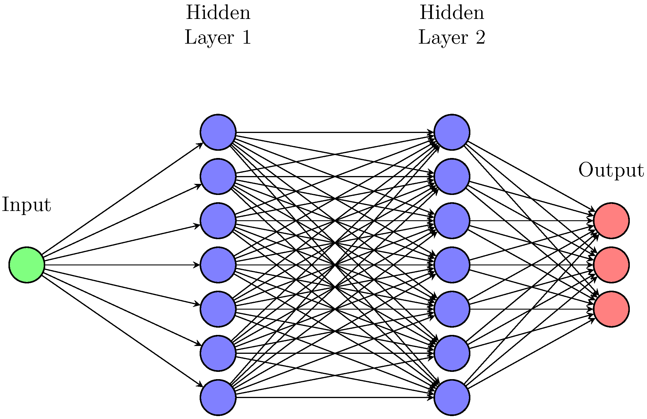
Figure 2. Neural network estimates and the measured data for the three competitors x , y , z.

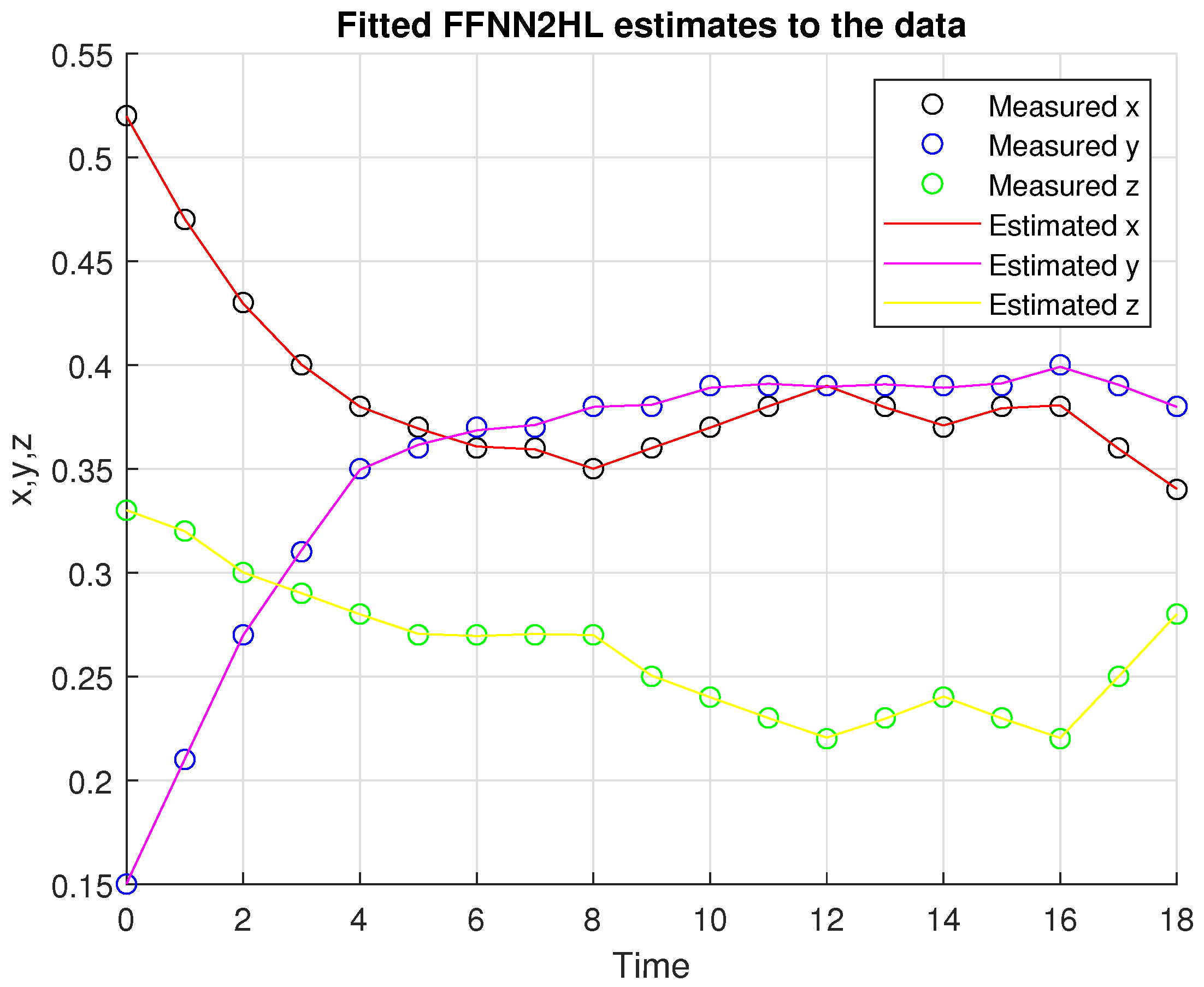
Figure 3. Comparison of the four methods with the measured data for the X competitor.

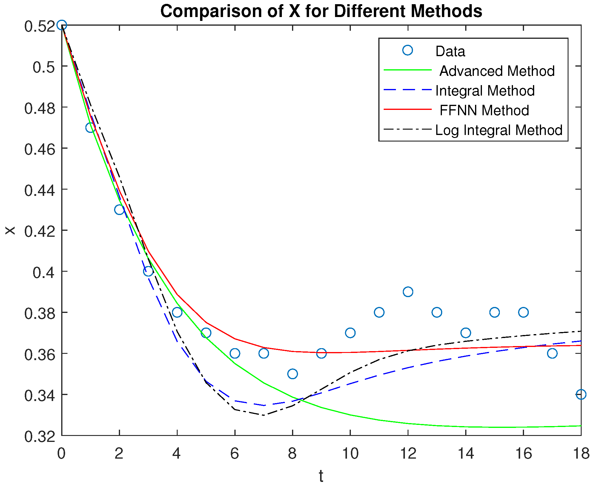
Figure 4. Comparison of the four methods with the measured data for the Y competitor.

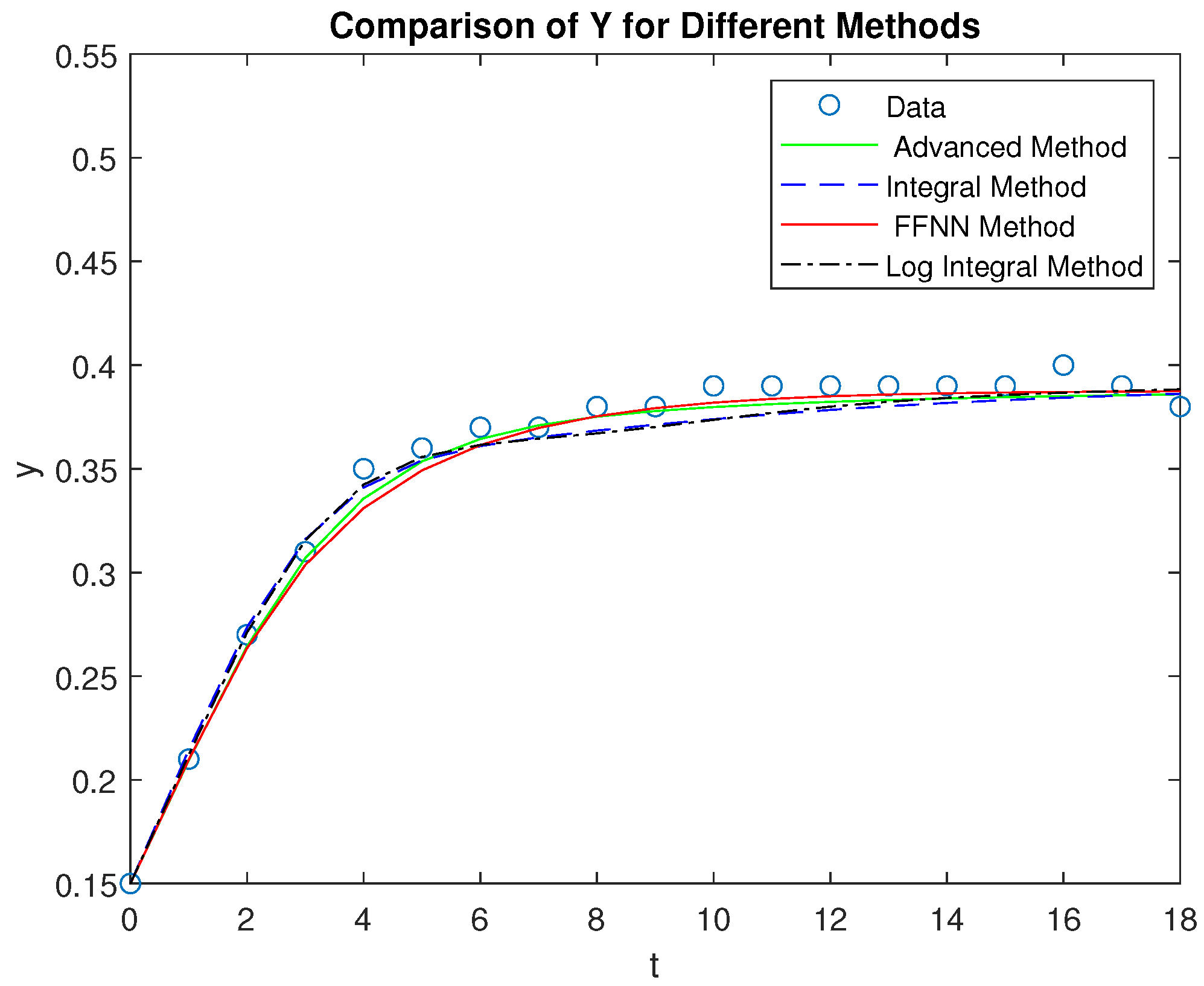
Figure 5. Comparison of the four methods with the measured data for the Z competitor.

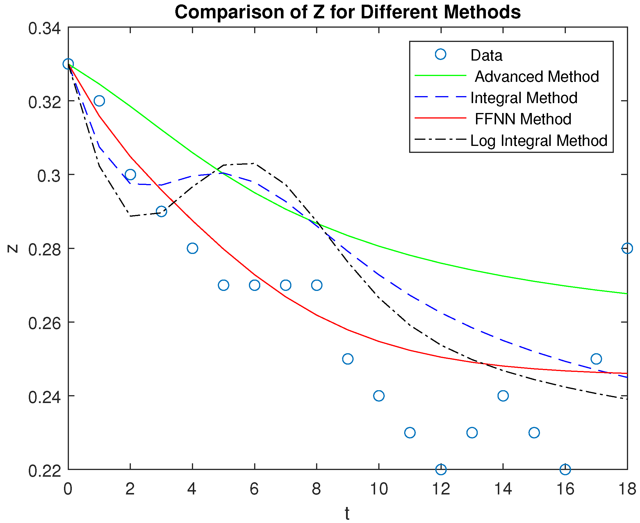
Table 1. Historical Market share data for competitors.

Period	Competitor x	Competitor y	Competitor z
1998a	0.52	0.15	0.33
1998b	0.47	0.21	0.32
1999a	0.43	0.27	0.30
1999b	0.40	0.31	0.29
2000a	0.38	0.35	0.28
2000b	0.37	0.36	0.27
2001a	0.36	0.37	0.27
2001b	0.36	0.37	0.27
2002a	0.35	0.38	0.27
2002b	0.36	0.38	0.25
2003a	0.37	0.39	0.24
2003b	0.38	0.39	0.23
2004a	0.39	0.39	0.22
2004b	0.38	0.39	0.23
2005a	0.37	0.39	0.24
2005b	0.38	0.39	0.23
2006a	0.38	0.40	0.22
2006b	0.36	0.39	0.25
2007a	0.34	0.38	0.28

* Data represents the market share for each competitor over various time periods.

Table 2. Root Mean Squared Error (RMSE) values for different methods and variables X, Y, and Z.

Method	RMSE for X	RMSE for Y	RMSE for Z
FFNN2HL	0.01304	0.00775	0.01549
Advanced	0.03449	0.00707	0.03206
Integral	0.01897	0.00894	0.02490
Log Integral	0.01871	0.00837	0.02324

Disclaimer/Publisher’s Note: The statements, opinions and data contained in all publications are solely those of the individual author(s) and contributor(s) and not of MDPI and/or the editor(s). MDPI and/or the editor(s) disclaim responsibility for any injury to people or property resulting from any ideas, methods, instructions or products referred to in the content.

© 2024 by the authors. Licensee MDPI, Basel, Switzerland. This article is an open access article distributed under the terms and conditions of the Creative Commons Attribution (CC BY) license (http://creativecommons.org/licenses/by/4.0/).

Copyright: This open access article is published under a Creative Commons CC BY 4.0 license, which permit the free download, distribution, and reuse, provided that the author and preprint are cited in any reuse.

Downloads

Views

Comments

Subscription

Notify me about updates to this article or when a peer-reviewed version is published.

MDPI Initiatives

Important Links

Choose an area of interest and we will send you notifications of new preprints at your preferred frequency.

Disclaimer

Neural Network-Based Parameter Estimation in Dynamical Systems

Abstract

Keywords:

Subject:

1. Introduction

2. Overview of the Lotka–Volterra Model Interpretation

3. Description of the Method

3.1. Data Collection and Normalization

3.2. Neural Network Architecture:

3.2.1. Feed-Forward Propagation

3.3. Training Process,Prediction and Denormalization

3.3.1. Back Propagation

3.3.2. Adam Optimizer

3.4. Prediction Process After Training

3.5. Parameter Estimation via Optimization

3.5.1. Mathematical Formulation of Quasi-Newton Method

3.6. Solving the System with Runge-Kutta method

3.6.1. Mathematical Formulation of the Runge-Kutta Method

4. Example

4.1. Case Study Description

4.2. Results and Comparison of the Four Methods

5. Conclusions

Author Contributions

Funding

Institutional Review Board Statement

Informed Consent Statement

Data Availability Statement

Conflicts of Interest

References

MDPI Initiatives

Important Links

Subscribe