1. Introduction
Time irreversibility, i.e., the invariance of a system or a time series under the operation of time reversal, has long attracted the attention of the statistical physics community [
1]; and, more recently, efforts have been devoted to its numerical quantification in real-world and experimental time series [
2]. Suppose a system for which we can observe its dynamics; if a given property of the latter is not the same in the normal (i.e., as observed forward in time) and time-reversed (i.e., observed backward in time) evolutions, we can then conclude that such system breaks time symmetry and is irreversible. Real-world experience provides uncountable examples of such time irreversibility: from ice cubes melting in a glass, to the mixing of initially separated gasses and liquids. Examples of time reversible systems are also easy to find, as e.g., the movement of an ideal pendulum. The interest in such concept is motivated by the fact that time irreversibility reflects, at a macroscopic scale, important mechanisms driving the dynamics of a system at a microscopic level. To illustrate, these include non-linear dynamics, (linear or non-linear) non-Gaussian dynamics [
3], the presence of dissipative forces (i.e., memory) [
4], and the departure from equilibrium [
5]. In other words, the observation of changes in the irreversibility of a system can indicate changes in the dynamics of the system itself, which may otherwise not be accessible to the researcher.
In the last two decades, many alternatives have been proposed to quantify irreversibility starting from real time series [
2]. Note that this problem is not trivial, as, firstly, the definition of irreversibility is agnostic with respect to the type of property that has to be evaluated; and, secondly, the extracted time series may represent only a part of the dynamics of the system - see Ref. [
2] for a detailed discussion. A complementary problem that (to the best of our knowledge) has hitherto not been tackled is the manipulation of the irreversibility. In other words, given a time series representing the dynamics of a system, our aim is to construct a modified version of the same of higher (or lower) irreversibility. The underlying hypothesis is a simple one: by analysing what are the most efficient ways of manipulating the irreversibility, one should be able to deduce which parts of the dynamics are driving it. Note that this idea, while being new in this context, is not new in general; for instance, a similar hypothesis buttresses tests on surrogate data, in which the objetive is to test and rule out specific explanations of an observed result [
6].
The problem of manipulating time irreversibility has trivial solutions. For instance, irreversibility is always reduced by noise [
7], e.g., observational one; and can be increased by introducing memory in the signal [
4]. Taking this to the extreme, a random permutation of any time series is reversible by construction, as any temporal structure is deleted; yet, such result is trivial and of no use. We here thus add an additional restriction, i.e., we aim at constructing time series of altered irreversibility that are maximally similar to the original one. This creates a trade-off between how much the time series has to be modified, compared to how much its time irreversibility is manipulated.
While numerous ways of performing such manipulation can be envisioned, we here propose to do this by applying the recently proposed concept of Continuous Ordinal Patterns (COPs) [
8]. These are a generalisation of the traditional ordinal pattern approach [
9], in which not only the relative order of data points but also their magnitudes is taken into account; and that have proven to be relevant in characterising time series, assessing irreversibility [
8], and improving causality tests [
10]. We propose a simple manipulation process in which, given a random COP, the time series is transformed according to it, and the result is discarded if it does not fulfil the required level of irreversibility; this is repeated a large number of times, for finally retaining the manipulated time series that has the highest linear correlation with the original one. COPs present several advantages in the context of the problem at hand. Firstly, as opposed to traditional ordinal patterns, COPs can be modified, hence the result is not only time series-dependent but also pattern-dependent. Secondly, the application of a COP is akin to a non-linear transformation, and is thus expected to increase the time irreversibility; yet, as will be shown, it can also effectively be used to reduce it. Finally, COPs are very efficient from a computational point of view, allowing the fast analysis of large sets of time series.
After introducing the concept of COP (
Section 2.1) and the numerical tests used to assess time irreversibility (
Section 2.2), we show how this property can easily be manipulated, both towards higher (
Section 3.2) and lower (
Section 3.3) values, while retaining a high similarity with the original time series. This is illustrated using time series of known irreversibility, generated by well-known chaotic maps and dynamical systems. We further illustrate how this approach can be used to probe the dynamics of real-world systems. Specifically, we show in
Section 4 how time series representing the brain activity of schizophrenic patients and matched control subjects initially have the same irreversibility; but that they yield significantly different results when manipulated. In other words, this pathology is modifying the normal brain dynamics by affecting its “distance to irreversibility”. We conclude with a discussion of the importance of these results in
Section 5, and further suggest future lines of research.
3. Results
3.1. Manipulating time series’ irreversibility through COP
We start this analysis by posing a basic question: supposing an initially time-reversible time series, does the application of a COP change such reversible nature? For that we consider a time series , and the corresponding transformation obtained by applying a random COP to it. For the sake of simplicity, in what follows we will assume that both time series are composed of n data points; note that in reality is shorter than by construction, but that this can easily be solved by considering the first n values of the latter. We further assume that is composed of independent random values, here drawn from a uniform distribution , such that it is time-reversible by construction. We then calculate the difference in the irreversibility of and , the latter measured by the p-value yielded by the four tests here considered when applied to both time series.
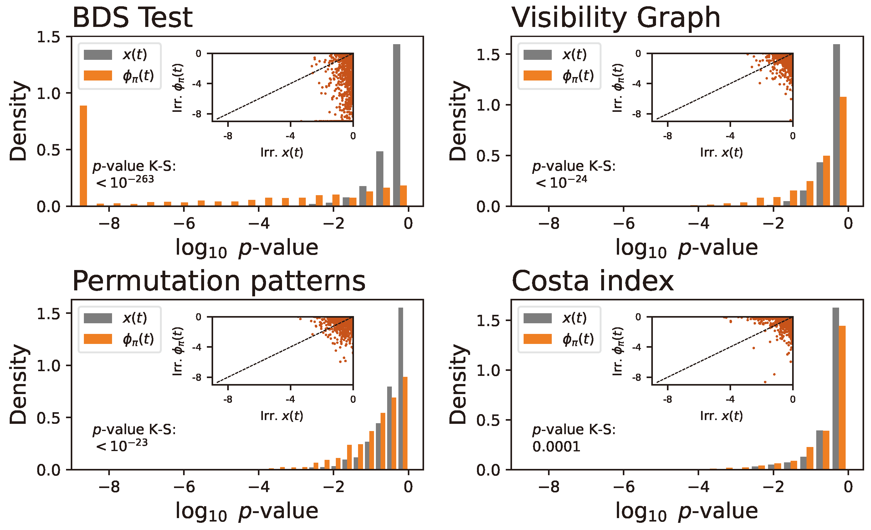
Figure 1 reports the probability distributions of the
of the
p-value, for
(grey bars) and
(orange bars), and for the four irreversibility tests. It can be appreciated that the
p-value is in general smaller, most drastically in the case of the BDS test. This is further confirmed by the insets, depicting scatter plots of the
of the
p-value of the transformed time series, as a function of the original one; and by two-samples Kolmogorov-Smirnov tests between the pairs of distributions, see
p-values inside each panel. In synthesis, it can be appreciated that the application of a random COP
generally results in an increase in the irreversibility of the time series, as initially hypothesised and in line with the non-linear nature of the transformation. This is nevertheless not always true: due to the stochastic nature of
, situations are observed in which the irreversibility is not changed, or is even reduced.
In order to get homogeneous results, we resort to the strategy proposed in Refs. [
8,
10], and involving the generation of a large set of random COPs
. For each one of them, the previous process is repeated, i.e., the time series is transformed into
and the irreversibility test is applied to it; finally, the transformation yielding the lowest
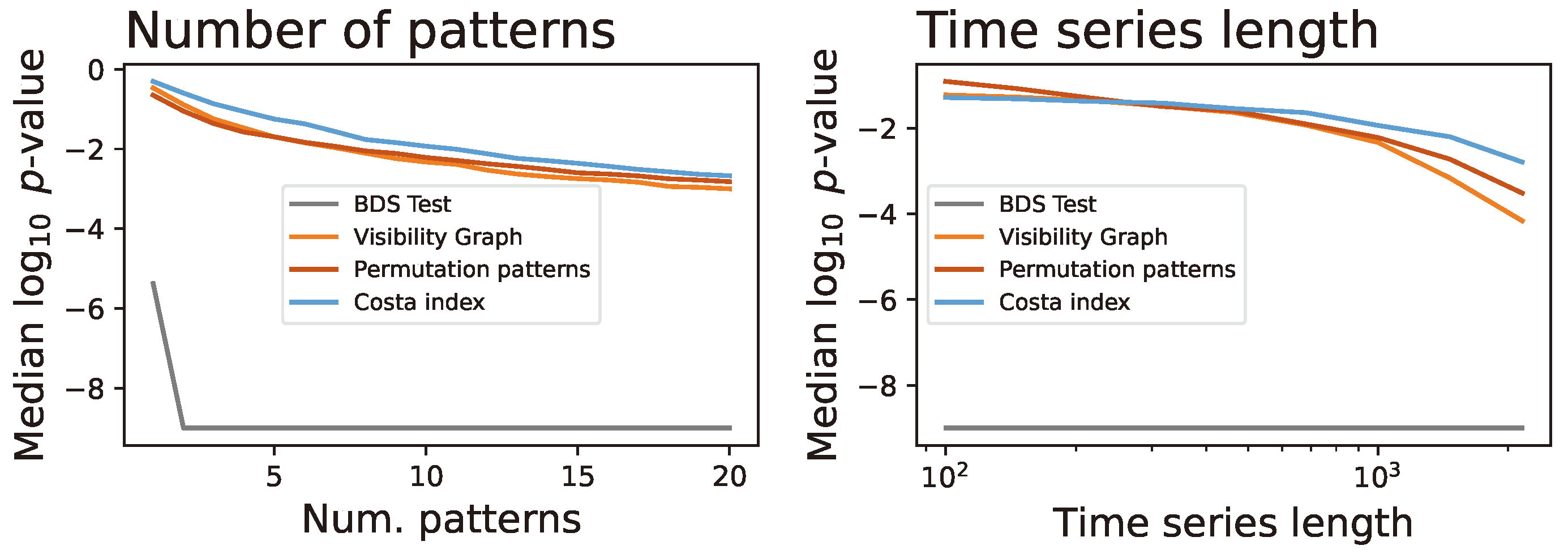
p-value (i.e., the highest irreversibility) is retained. The left panel of
Figure 2 reports the evolution of the median of the obtained
p-values, as a function of the number of generated random patterns. It can be appreciated that 20 random patterns are enough to obtain time series that are irreversible in a statistically significant way (i.e.,
p-value
) in the majority of cases. It is also interesting to observe the wide difference between the BDS test on one hand, and all other tests in the other; this is due to the fact that the former does not only assess irreversibility, but is rather design to detect the presence of non-linearities in general. We finally evaluated the role of the time series length, obtaining that longer time series are associated to slightly smaller
p-values, see right panel of
Figure 2.
The results presented in
Figure 1 and
Figure 2 thus confirm that, as initially hypothesised, the application of COPs can increase the irreversibility of a time series - and make it more non-linear, as suggested by the different behaviour of the BDS test compared to the remainder ones. This increase is generally weak and further stochastic in nature; yet, stable results can be obtained by performing the same process multiple times.
3.2. Increasing irreversibility with minimal changes
Can the previous approach be used to increase the irreversibility of time series without substantially changing their dynamics? In order to tackle this question, we have modified the previous approach to include an assessment of the similarity between and . More in details, we firstly create a large set of random COPs (here ); each one of them is applied to the original time series, and discarded whenever the p-value yielded by the irreversibility test is above a given threshold (here ). We next calculate the linear correlations between and the time series created in the previous step; the pattern for which such correlation is maximal in absolute value is finally selected as the best one. Note that this guarantees that the transformed time series is both irreversible (with a p-value ), and at the same time maximally similar to . In order to include more flexibility in this process, we further create a new time series by linearly combining the original and the transformed time series, i.e., , with . By varying the mixing parameter between 0 and 1, morphs between the two time series; this can be used to balance the output between time series very similar to the original one (with ), or maximally time irreversible (with ).
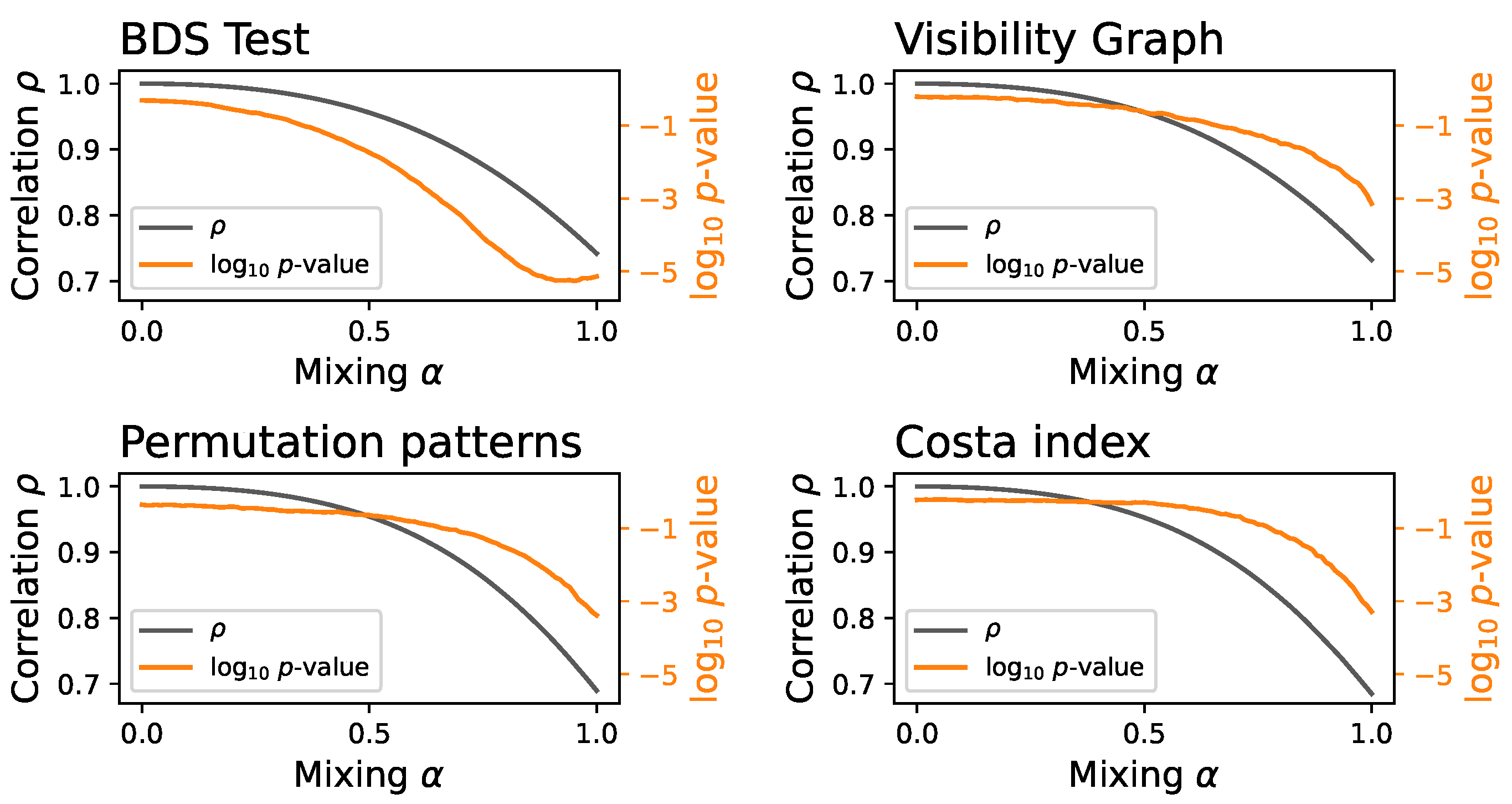
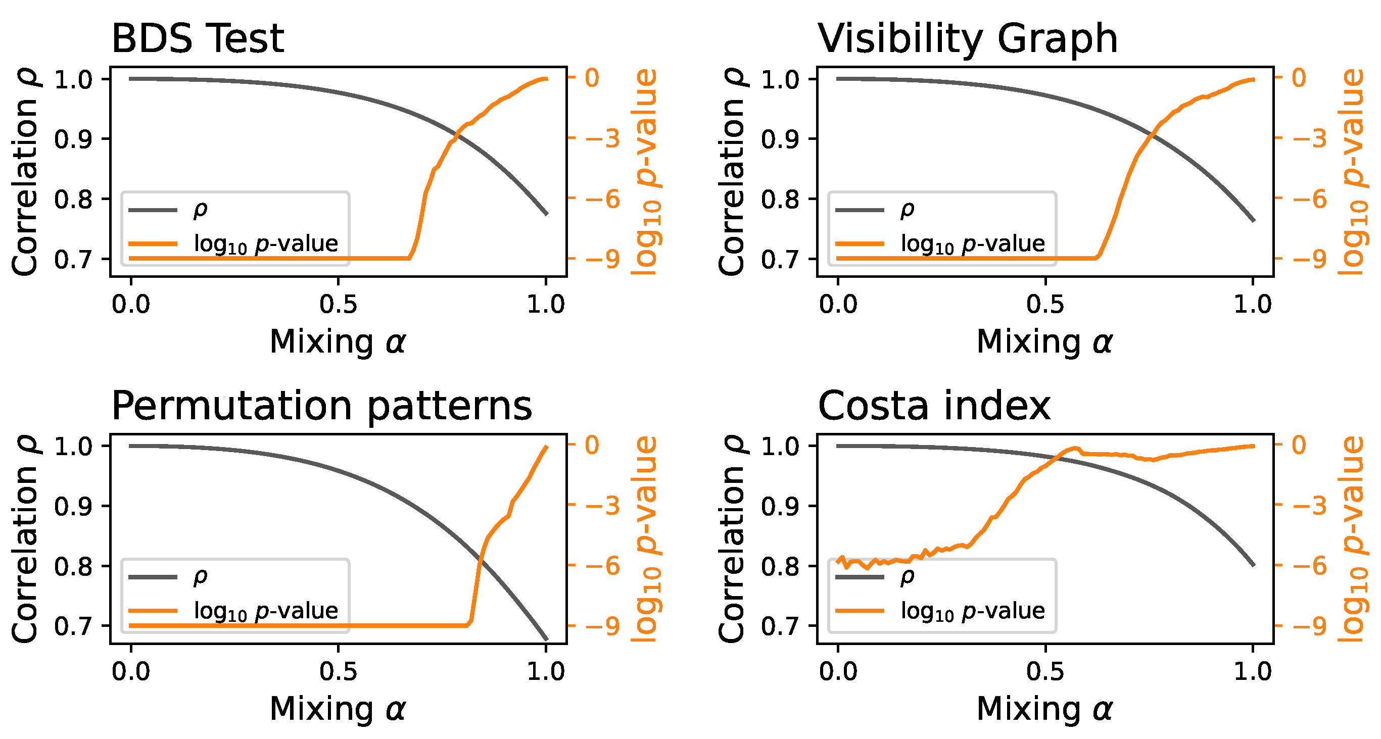
Figure 3 reports the evolution of the correlation coefficient
between
and
, and of the median of the
of the
p-value of the irreversibility test applied to
, as a function of the mixing
. It can be appreciated that, as
increases, the resulting time series are more irreversible but also less similar to the original one - as expected by construction. Still, in all cases it is possible to find a value of
for which the
p-value is below
(i.e., the time series can be considered irreversible) while still displaying a
.
The results of
Figure 3 were obtained starting from time series
comprising random values drawn from a uniform distribution
. In order to check their generalisability,
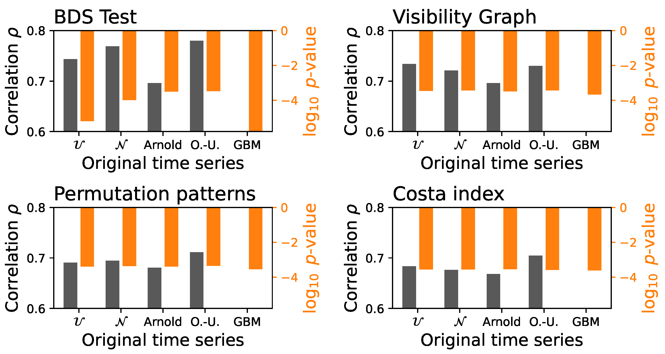
Figure 4 reports the two same metrics, for
, for:
: The same uniform distribution , included as a reference.
: Random values drawn from a normal distribution .
Arnold: Time series corresponding to the
x variable of an Arnold map, a chaotic and conservative (hence, reversible) map, defined as:
O.-U.: Ornstein-Uhlenbeck process, i.e., a mean-reverting linear Gaussian process [
3].
GBM: Geometric Brownian motion described by the following Langevin equation [
23]:
where
is the Wiener increment of zero mean
and correlation function
; and
the drift amplitude. By setting
, the resulting time series is stationary and reversible [
24].
As can be seen in
Figure 4, all cases behave mostly similarly; the notable exception is the GBM process, yielding a very low correlation coefficient (always below
, not reported for the sake of clarity). In other words, starting from time series that are time reversible, the final result of the process can be different. Taking into account that the optimisation process is the same in all cases, this indicates that different time series are differently predisposed to become irreversible, or that the efficiency of the process changes depending on the nature of the analysed time series; in other words, that a “distance to irreversibility” can be defined. This will further be used in
Section 4.
3.3. Reducing irreversibility
Up to here we have focused on the problem of manipulating (initially reversible) time series to artificially increase their irreversibility, obtaining generally good results. The question that naturally follows is: can the process be reversed? That is, starting from irreversible time series, is it possible to manipulate them to obtain reversible ones? While this can trivially be obtained by adding some observational noise, we here want to see if the previous methodology can yield similar results.
The previous approach has been modified towards this aim. On the one hand, we start from irreversible time series generated with the chaotic Logistic map:
, with
. Being a dissipative map, the resulting time series are irreversible by construction [
25]. On the other hand, manipulated time series are retained whenever the
p-value yielded by the irreversibility test is above a threshold of
- i.e., to guarantee that they are time-reversible.
Figure 5 presents results similar, albeit slightly worse, than the previous case. Specifically, with values of
close to 1, it is possible to obtain reversible time series, with correlations between
and
. The fact that lower correlations are obtained is not surprising, considering that the transformation induced by COPs is a non-linear one; this transformation thus naturally tends towards higher irreversibilities, and is here applied to obtain the opposite result. Additionally, and as previously mentioned, irreversibility can easily be reduced by introducing noise in the time series. We tested this idea by starting from time series generated with the Logistic map, for then adding noise drawn from a uniform distribution until the irreversibility felt below what obtained by the proposed transformation.
Figure 6 then reports the average
, as obtained when introducing noise, as a function of the one obtained with the COP manipulation. Results are similar, except in the case of the Costa index: small quantities of noise are enough to confound this test and obtain large
p-values, consequently obtaining time series very similar to the original ones. In synthesis, while the addition of an observational noise may be more efficient, the proposed optimisation procedure is still valid to reduce the irreversibility of time series.
4. Manipulation of the time irreversibility of brain dynamics
One interesting conclusion that can be inferred from
Figure 4 is that the manipulation process here proposed does not yield the same result depending on the characteristics of the original time series. For instance, for all four irreversibility tests, the resulting
is higher when the starting point is a time series created by the Ornstein-Uhlenbeck process, but substantially lower in the case of the Geometric Brownian Motion. Therefore, even if both types of time series are originally time-reversible, they have a different predisposition to be manipulated towards a higher irreversibility. In turn, this means that the result of the manipulation process can be used as a way of characterising the time series, beyond what a direct analysis of their irreversibility would yield.
In order to test this idea, we here analyse time series representing human brain activity. The computation performed by the human brain necessarily relies on non-linearities and memory; the underlying dynamics may thus be expected to be time irreversible. At the same time, we do not have direct access to such dynamics, but only to indirect measurements of it (e.g., through electroencephalography); and these are usually coarse-grained and noisy. As a result, irreversibility and its variation across conditions and pathologies can only reliably be measured in long time series [
26,
27,
28].
We have considered the data set freely available at
http://dx.doi.org/10.18150/repod.0107441 and described in Ref. [
29], consisting of electroencephalographic (EEG) recordings in a rest condition of 14 patients suffering from schizophrenia, and of the same number of matched control subjects. The patients (7 males,
years, and 7 females,
years) met the International Classification of Diseases ICD-10 criteria for paranoid schizophrenia (category F20.0); on the other hand, the healthy controls were 7 males (age of
years) and 7 females (age of
). The EEG data correspond to an eyes-closed resting state condition, and were recorded at 250Hz using the standard 10-20 EEG montage with 19 EEG channels: Fp1, Fp2, F7, F3, Fz, F4, F8, T3, C3, Cz, C4, T4, T5, P3, Pz, P4, T6, O1, O2. The reference electrode was placed at FCz. No additional preprocessing steps (e.g., artefact removal) have been performed, beyond what was initially included in the original study [
29].
We start by calculating the irreversibility of these time series, by randomly extracting 100 short segments (of 100 points, i.e.,
seconds) for the Fp2 channel from all subjects, and obtaining
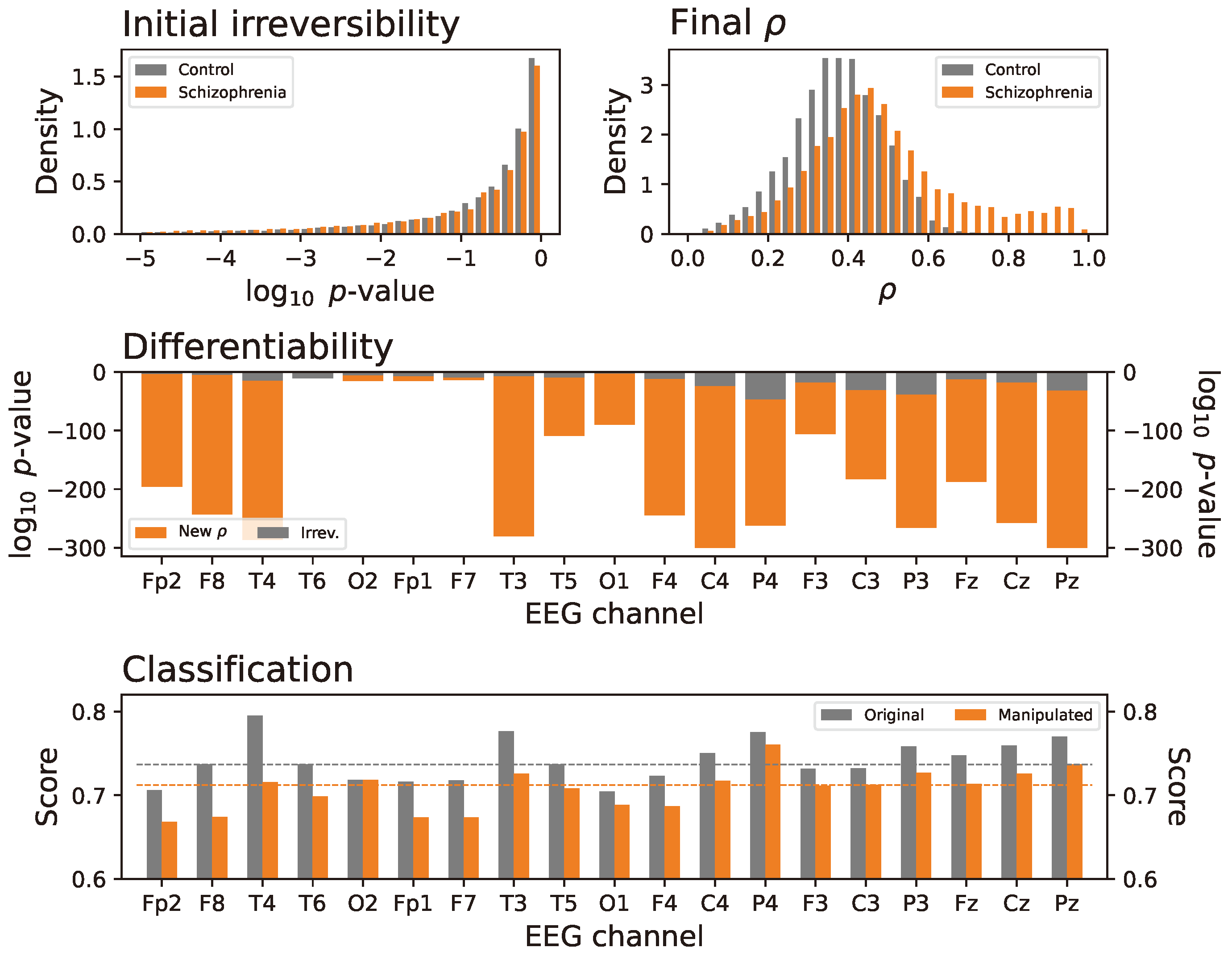
p-values according to the Costa index test. As can be appreciated in the top left panel of
Figure 7, most segments are time-reversible, and almost no differences are present between the two conditions. We then applied the manipulation procedure described in
Section 3.2, aimed at increasing the irreversibility of these time series, and evaluated the resulting
between the manipulated and original segments. The results are represented in the top right panel of the same figure, and suggest the presence of a significant difference between both groups. In other words, even if both groups of segments have the same initial irreversibility, they present different distances to irreversibility; and this is smaller (i.e., manipulations of smaller amplitudes are needed to reach irreversibility, hence yielding a higher
) for schizophrenic patients. Such difference between control subjects and patients is statistically significant, as measured by a two-samples Kolmogorov-Smirnov test between both distributions; and is further stable across most EEG channels - see middle panel of
Figure 7.
If the manipulated time series display a larger difference between the two groups in terms of time irreversibility, does it mean that they are more identifiable? In order to answer this question, we have trained a Deep Learning (DL) model to discriminate between the two groups. Such model is the Residual Networks (ResNet) [
30], i.e., a convolutional architecture that introduces the possibility of skipping connections between layers, allowing the network to learn residual functions and mitigate the vanishing gradient problem of very deep networks. This has been chosen for its high efficiency in classifying sets of time series [
31,
32]. Key hyperparameters include the number of blocks (here set to 5), each comprising 5 layers of 32 filters of size 10. The bottom panel of
Figure 7 reports the average classification score (i.e., the fraction of time series whose group was correctly identified by the ResNet model) for each EEG channel, when the model is trained and tested using the original (grey bars) and manipulated (orange bars) time series. Notably, the original time series yield larger classification scores across all channels - see also the median across them, represented by the dashed horizontal lines. In other words: even though the manipulation process allows to obtain time series that are more different between the two conditions in terms of irreversibility, these are less different in general.
As a final test,
Figure 8 reports the results when modifying time series corresponding to the Fp2 channel with the aim of reducing the time irreversibility; in other words, the two panels in
Figure 8 correspond to the same panels in
Figure 7 when applying the procedure described in
Section 3.3. Notably, the results are very similar, with time series corresponding to schizophrenic patients being also easier to modify towards a reduced irreversibility.
5. Discussion and conclusions
While many tests have hitherto been proposed for the assessment of the time irreversibility of real-world time series [
2], less attention has been devoted to the problem of manipulating this property. We have here analysed one possible approach for this, specifically using the concept of Continuous Ordinal Patterns (COP) [
8]. In other words, given a time series, we here aimed at increasing (or decreasing) its irreversibility, while at the same time retaining its original dynamics (as measured by a linear correlation). The reader interested in reproducing the results will find a Python implementation of the algorithm available at
https://gitlab.com/MZanin/irreversibilitytestslibrary. After proving that this is feasible in synthetic time series (
Section 3.2 and
Section 3.3), we moved to the analysis of human brain data (
Section 4).
As shown in
Figure 4 and
Figure 7, the proposed manipulation process allows to describe time series through a new concept: the distance to irreversibility. Specifically, suppose two time series that are both described as time-reversible by a given test; they may require modifications of different intensities to reach irreversibility, resulting in different values of
(i.e., the correlation between the original and manipulated versions of the time series). As demonstrated in the case of brain time series, this may be useful to discriminate between different conditions. These results lead to two interesting questions, which have hitherto never been tackled in the literature.
Firstly, what does this “distance from irreversibility” represent? While it may be tempting to interpret this as an amount of irreversibility, or the distance of the system to equilibrium, it is worth noting that such amount would manifest as differences in the initial
p-values obtained by the tests. In other words, the time series analysed in
Section 4 are very similar from an irreversibility point of view, are should therefore represent conditions in the brain with a similar distance to equilibrium. Two alternative explanations can be proposed. On the one hand, that the time series have actually different levels of irreversibility, which are nevertheless masked by the limited lengths of the considered segments. This is aligned with previous results indicating that long time series are required to detect irreversibility in EEG data [
26]; yet, this seems at odd with the fact that time series of schizophrenic patients are more easier moved towards both higher and lower levels of irreversibility, see
Figure 7 and
Figure 8. On the other hand, this can be interpreted by the amount of modifications that are required to start moving the dynamics towards a desired level of irreversibility, i.e., how much the dynamics has to be modified to increase (or decrease) the amount of entropy it produces. Note nevertheless that the dynamics of the system is not changed, but rather the evolution of the observable used to describe it; hence, this distance tells us under which observational lens the system has to be observed to become time reversible or irreversible.
Secondly, what does this “distance from irreversibility” represent in a neuroscience context? It is clearly related to different forms of working of the brain, as shown by the important differences between control subjects and schizophrenic patients (
Figure 7). Yet, what those differences are, and how they are related to the underlying pathology, are still open questions that ought to be tackled in the future.
Figure 1.
Comparison of the probability distributions of the
of the
p-values, for respectively the original time series
(grey bars), and the transformation
(orange bars). Each panel reports the results for an irreversibility test, as described in
Section 2.2. The insets further depict scatter plots of the
of the
p-values of
, as a function of those of
; for reference, the dashed grey line represents the main diagonal. Finally, the text in each panel reports the
p-value of a two-sample K-S test between the two probability distributions. Results correspond to time series of length
.
Figure 2.
Using multiple random patterns. (Left) Evolution of the median of the p-values obtained by each test (see legend for colour codes) on the transformed time series , as a function of the number of random patterns considered, and for time series of length . (Right) Evolution of the same metric as a function of the time series length, when 10 random patterns are used.
Figure 3.
Increasing the irreversibility of random time series. Evolution of the linear correlation coefficient between and (left Y axis, grey lines), and of the of the p-values obtained by each irreversibility test on (right Y axis, orange lines), as a function of the mixing parameter - see main text for details.
Figure 4.
Linear correlation coefficient (left Y axes, grey bars) between the original and manipulated time series, and of the p-values (right Y axes, orange bars) obtained by each irreversibility test on latter time series, as a function of the type of time series.
Figure 4.
Linear correlation coefficient (left Y axes, grey bars) between the original and manipulated time series, and of the p-values (right Y axes, orange bars) obtained by each irreversibility test on latter time series, as a function of the type of time series.
Figure 5.
Reducing the irreversibility. Evolution of the linear correlation coefficient between and (left Y axis, grey lines), and of the of the p-values obtained by each irreversibility test on (right Y axis, orange lines), as a function of the mixing parameter - see main text for details.
Figure 5.
Reducing the irreversibility. Evolution of the linear correlation coefficient between and (left Y axis, grey lines), and of the of the p-values obtained by each irreversibility test on (right Y axis, orange lines), as a function of the mixing parameter - see main text for details.
Figure 6.
Scatter plots of the
obtained by adding random noise, as a function of the
obtained in the COP manipulation process. Each point corresponds to a different value of
; and noise is added to the original time series until the same level of reversibility of
Figure 5 is achieved.
Figure 6.
Scatter plots of the
obtained by adding random noise, as a function of the
obtained in the COP manipulation process. Each point corresponds to a different value of
; and noise is added to the original time series until the same level of reversibility of
Figure 5 is achieved.
Figure 7.
Manipulating irreversibility in the brain. (Top left) Probability distributions of the p-value obtained when applying the Costa index test, for control subjects (grey bars) and schizophrenic patients (orange bars), to time series corresponding to the Fp2 EEG electrode. (Top right) Probability distributions of obtained after the manipulation of the same time series, for control subjects (grey bars) and schizophrenic patients (orange bars). (Middle) Orange bars: p-value yielded by a K-S test, comparing the distributions of for control subjects and patients (i.e., what depicted in the top right panel). Grey bars: p-value yielded by the same test when applied over the distributions of irreversibilities (i.e., what depicted in the top left panel). (Bottom) Score obtained by a ResNet model when trained to discriminate between control subjects and patients, using the original (grey bars) and manipulated (orange bars) time series.
Figure 8.
Reducing irreversibility in the brain. (Left) Probability distributions of the p-value obtained when applying the Costa index test, for control subjects (grey bars) and schizophrenic patients (orange bars). (Right) Probability distributions of obtained after the time series manipulation aimed at reducing the time irreversibility, for control subjects (grey bars) and schizophrenic patients (orange bars). All results correspond to the Fp2 channel of the EEG data.
