Graph-based Analysis for the Characterization of Corrugated Boards Compression

This paper proposes a novel approach to represent the geometry of the corrugated board profile during compression by using graphs. Graphs are lighter than images, and the computational time of compression analysis is then significantly reduced compared to using the original image data for the same analysis. The main goal of using such graphs is to gain more knowledge about the mechanical behavior of corrugated boards under compression compared to the current load-deformation curve approach. A node-tracking algorithm is applied to characterize the different phases happening during the compression test in order to predict physical phenomena, including buckling and contact. The main results show that analyzing the nodes provides significant insights into the compression phases, which was not achieved in the current state-of-the-art. The authors believe the object of this research is crucial to better understand the physics of corrugated boards under compression, and it can also be extended to other engineering structures.

Keywords:

Subject:

Engineering - Mechanical Engineering

1. Introduction

Corrugated board is one of the most popular and in-demand materials in the packaging sector. It is lightweight, affordable, and offers good protection and cushioning for the objects being transported [1,2]. Additionally, it provides effective and sustainable packaging options that are in great demand across a variety of industries, including e-commerce, pharmaceuticals, cosmetics, food and beverage [1,3,4]. It is a highly recyclable and biodegradable material as well. Enhancing the understanding of corrugated board mechanical behavior under compression aids in product design optimization by lowering the product’s weight and cost and by boosting its capacity to absorb energy. Packages with such ideal designs are less expensive and lighter yet are able to provide cushioning. A further area of optimization that can be studied is the prediction of energy absorption and corrugated board failure.

Shape and topology optimization in corrugated boards have not yet been thoroughly examined in the literature, [1] and modeling approaches to tackle those challenges should be investigated since these may enhance the robustness and applicability of the findings. In the optimization process, reliability in terms of computational efficiency is crucial. Finite element models were utilized in earlier studies [5,6] to simulate deformation and analyze stress in the corrugated board under out-of-plane compression. The Flat Crush Test (FCT) is the equivalent test. While being accurate, Finite Element Method is computationally expensive. Also, the only reliance on FEM-modeling that dominates in the field of corrugated board would make the accuracy and reliability of optimization solutions strongly dependent on the precision of models [1], where the fluting medium is approximated by an ideal sine wave, which, for example, does not replicate the symmetry imperfections in the real sample, due to the sole reliance on FEM-modeling that is dominant in the field of corrugated board. Experimental testing of samples yields a load-deformation curve that characterizes the general behavior of the board and provides additional information about the compressive behavior of the corrugated board. It does not, however, offer details regarding local stresses and deformations.

An image analysis could be investigated in order to close the gaps described earlier. It is not ideal to use raw photos in optimization studies since they contain an excessive amount of data that needs to be stored and analyzed. Consequently, it can be beneficial to reduce the dimensionality of picture data by summarizing the most crucial information in the image using graphs. A similar goal of dimensionality reduction is achieved in the literature by using graphs [7,8] to effectively describe data distribution or structure. Efficient analysis of corrugated board images in terms of both time and data storage is carried out by taking into account the graph representation of the board geometry. Compared to raw photos, graphs contain a lot less data, but they provide more about the profile shape than the experimental load-deformation curve does. They serve to condense the profile geometry, which is the most significant piece of information in the image. Further information about the deformation and buckling behavior of the fluting structure can be obtained by tracking the nodes in the graphs and calculating their displacement.

In this work, a novel method for graph-based image analysis of corrugated boards under compression is proposed. An image of the profile geometry will reproduce the symmetry defects of the fluting medium based on pictures of actual samples under compression.

The aims of this method are as follows:

Reducing the dimensionality of corrugated board images by using graphs.
Gaining more information about the mechanical behavior of corrugated boards in comparison to the load-deformation curve.

The remainder of the paper is as follows: In section 2, the state of the art about image analysis in corrugated boards and in other fields is presented; section 3 presents the materials and methods that are used in this paper; section 4 presents and discusses the results achieved based on the applied methodology and the limitations are tackled; section 5 summarizes the most relevant of the results and makes reference to future works.

2. State of the Art

An image analysis based on the genetic algorithm was applied to corrugated board profiles in a recent work conducted by Rogalka et al. [9] The goal was to calculate an estimation of geometric features, namely thicknesses of different layers, centerline, period, and initial phase of the fluting medium that was approximated by a sine wave. Later, the same analysis was applied on double-walled corrugated board.[10] Geometric features could be identified precisely in the case of non-crushed board and with less precision when the same procedure is applied to crushed samples. The effectiveness of the procedure is highly dependent on the quality of the sample cross-section. The same authors applied a Convolutional Neural Network (CNN) for the classification of 7 different types of corrugated board [10]. The algorithm was highly efficient and achieved, in some cases, more than 99% accuracy. Classification of crushed samples was also possible, highlighting the robustness of CNN applications. In a later work, two classification methods of corrugated boards based on cross-section images were compared. The first method used was a genetic algorithm to identify geometric features and a simple feedforward neural network. The second method is based on the already mentioned CNN application. The second method was found to be more efficient in both precision and inference time. [11]

In several other works, still related to corrugated boards, [12,13,14] algorithms were developed for the automatic counting of stacked corrugated boards based on images of the profile side of corrugated board stacks and also the slitter side, where the corrugation is not depicted. The results of the developed procedures are satisfactory and can potentially help automate the counting task in the production and quality control of corrugated boards. Later, an algorithm was developed to combine corrugated board images using image stitching techniques and feature tracking. This was applied to images of the profile side of corrugated board stacks. For corner detection, the Forstner method was used. The RANSAC method was applied to correspond to the features detected. The combination of images was then performed with bundle adjustment. Results showed that cardboard images are correctly combined when at least 25% overlapping was given. The number of board sheets was also correctly calculated based on the stitched image. [13]

In other words not related to corrugated boards but still related to the method presented here, methods of image analysis were applied for the deformation characterization of materials under given load or displacement conditions. An algorithm based on Digital Image Correlation (DIC) was proposed by Radi et al. [15] for the deformation tracking of truss lattices under dynamic loading. Depending on the truss type, a grid was first generated to define points of interest in the structure. During a compression test of the structure, the nodal displacement of these points of interest was tracked using a DIC-based algorithm. It was shown that optimal results highly depend on the choice of imaging frame rate. Measurement error was proven to be under 1 pixel for the tested trusses, which highlights the high efficiency of the procedure.

Image analysis methods were also used to track the deformation in honeycomb structures. As an example, the work of Hu et al. [16] is mentioned. Image skeletonization and a branch point matching algorithm were employed to track the deformation of honeycomb structures under compression and tension. Calculating the mean bias errors in the simulations showed that the algorithm attains sub-pixel precision. Additionally, a correct matching of branch points on branches with imperfections was attained, which proves the accuracy and robustness of this procedure when applied to honeycomb structures.

Liang et al. [17] developed an image analysis procedure to determine the curvature of continuous fiber-reinforced material in a bending test. It was based on binarization and skeletonization of the transverse cross-section image of a sample during a bending test. The curved geometry of the material was represented by approximating some points of interest on the cross-section using a uniform quartic B-spline. After the curvature values are determined, a bending moment-curvature curve was elaborated successfully.

3. Materials and Methods

3.1. Graphs

Graphs are a type of data that helps define and visualize relations between various components. They are used in various fields like mathematics, computer science, and data science. A graph is a set of nodes and edges between some node pairs. As defined by Diestel [18]:

"A graph is a pair $G = (V, E)$ of sets such as $E \subseteq {[V]}^{2}$ ; thus, the elements of E are 2-element subsets of V. The elements of V are vertices (or nodes, or points) of the graph G, the elements of E are its edges (or lines)."

Some of the main terminology in graphs are the concepts of order, neighbors, degrees, and paths. The order of a graph is equal to the total number of nodes it contains, i.e., the number of elements in V, and it is denoted by

| G |

. The number of edges is denoted by

∥ G ∥

. [18]

Two vertices x and y are neighbors if

(x, y)

is an edge in E. [18] The degree of a vertex v is written as

d_{G} (v)

and is equal to the number of edges related to v. By the already mentioned definition of a graph, the degree of a node is always equal to the number of neighbors it has. [18] This would not be valid in the case of multigraphs, where more than one edge is allowed between two nodes.

A path defined as a non-empty graph of the form

V = {x_{0}, x_{1}, . . ., x_{k}}

and

E = {x_{0} x_{1}, x_{1} x_{2}, . . ., x_{k - 1} x_{k}}

, where

x_{0}

and

x_{k}

are the ends of the path. In more common sense, a path is the sequence of nodes that lead from a start node

x_{0}

and a node

x_{k}

. The length of a path is equal to the number of edges that are traversed when the path is followed. [18]

Some of the principal types of graphs are directed vs. undirected, connected vs. disconnected, weighted, and simple graphs. A graph is connected if there exists at least one path relating to every two nodes in that graph. Otherwise, the graph is disconnected. [29, p. 6] Directed graphs have edges with a specific direction so that the edges

(u, v)

and

(v, u)

are not equivalent. In undirected graphs, edges do not have a specific direction. As a result,

(u, v)

and

(v, u)

are equivalent. Weighted means that different numbers are attributed to the edges. In unweighted graphs, all edges are considered equally weighted by 1. A graph is simple if there are no self-loops, i.e., edges of the form

(u, u)

, nor multi-edges, i.e., more than one edge between two nodes. [19]

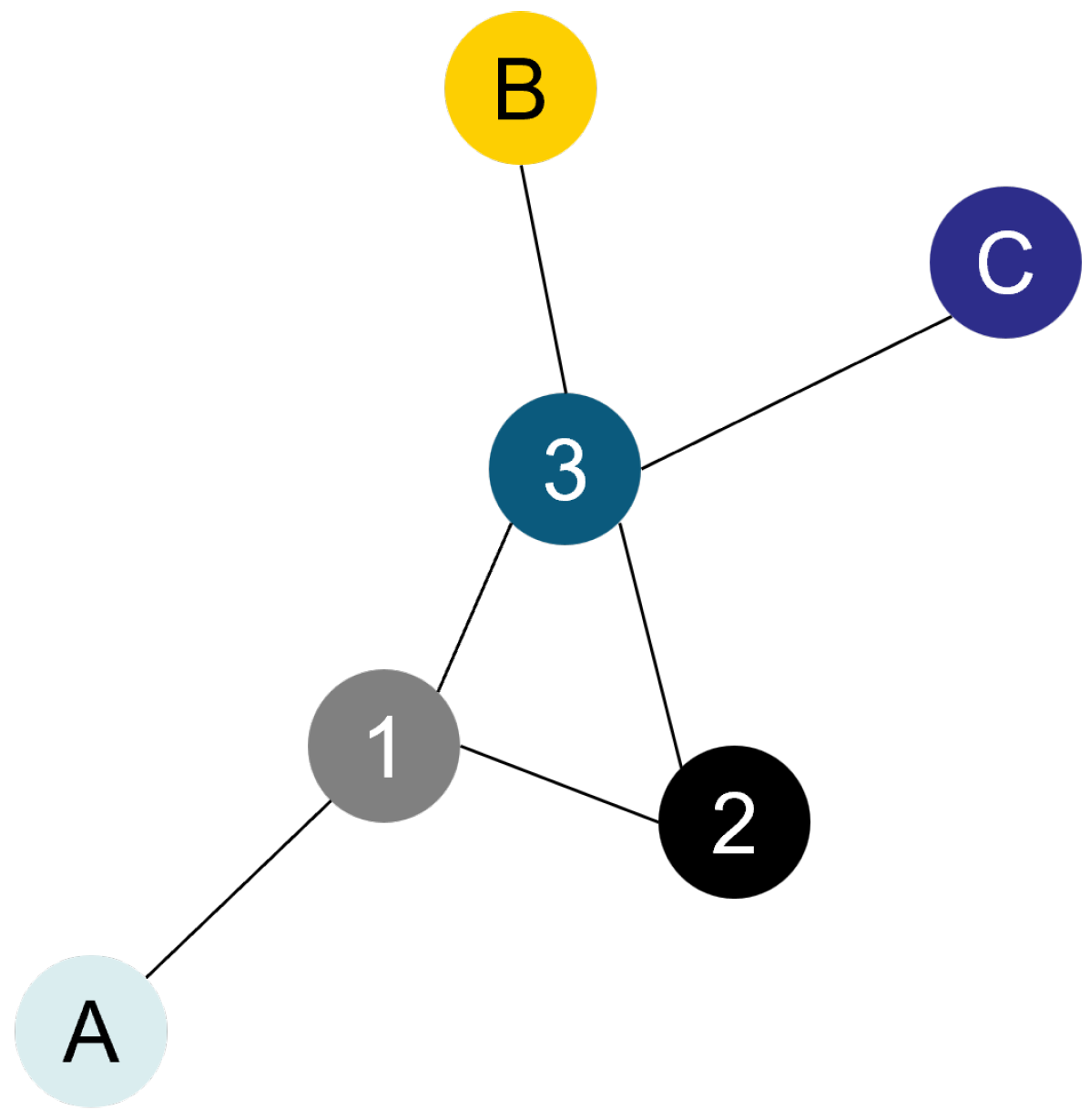
An example of an undirected, connected, and simple graph is illustrated in Figure 1. Its order is 6, which is the number of nodes it has. The sets of vertices and edges are respectively:

V = {1, 2, 3, " A ", " B ", " C "}

E = {(1, " A "), (1, 2), (1, 3), (2, 3), (3, " C "), (3, " B ")}

For example, the set of neighboring nodes of node 1 is

{" A ", 2, 3}

, and the degree of node 1 is then

d_{G} (1) = 3

3.2. Methodology

A methodology to reduce the data dimensionality of corrugated board images by employing graphs is proposed and presented in this section. The flowchart in Figure 2 illustrates the steps of the methodology. In subsection 3.3, the gathering method of the experimental data is presented. A video is acquired by using a camera, and images are extracted from the video and subjected to pre-processing and filtering. The filtering process is presented in subsection 3.4. In section 3.5, the process of getting the graphs from filtered images is detailed.

3.3. Experiment Setup

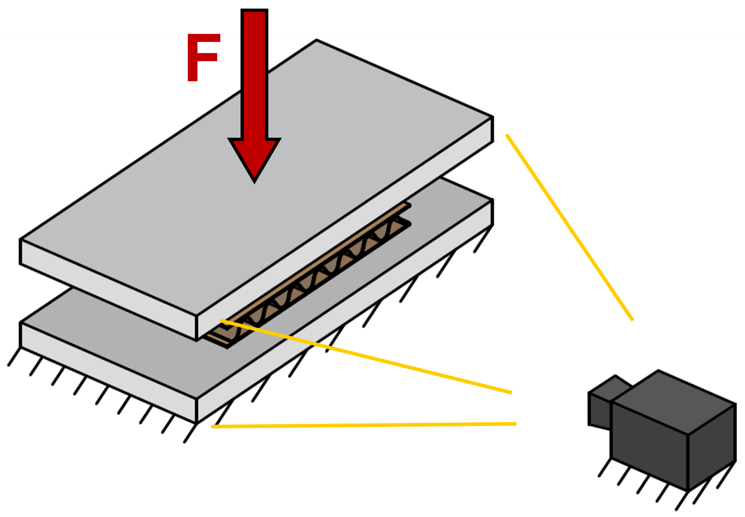
A compression test was performed on corrugated board samples, which were loaded perpendicular to their surface. A Zwick machine is used for this purpose. A gray-scale camera is mounted on a frame that is connected to the machine housing. The model of the camera is “Vosskühler HCC - 1000/512s". An objective lens “NIKKOR 50mm 1:1.4" with a focal length of 50 mm and a Teleconverter “Nikon TC - 201 2x" to double the focal length are used. A video of the corrugated board cross-section during the compression test is recorded. It has a resolution of 256 x 1024 pixels. One pixel represents

87 \pm 2 μ m

. A self-made LED light source is used to illuminate the profile of the specimen. It is made of 2 sets of LEDs, each having a maximum power of 100 W. A laboratory generator is used as a power supply for the LED lights. The voltage is set to 28 V, which results in a power of 40 W. Camera and lens parameters, like for example the Depth of Field (DoF) and the exposure time, are manually adapted, to obtain a sharp and well-illuminated image. A simplistic representation of the process is done in Figure 3.

Samples are conditioned in laboratory conditions of humidity and temperature of

50 \pm 2 %

and

23 \pm 1^{\circ} C

, respectively. Tests were performed in the same laboratory conditions and under LED lights only. This way, the videos recorded have a dark background, and the thin-walled structure of the corrugated board profile can be well depicted. The compression test is performed using a prescribed displacement, with a constant movement speed of the upper compression plate set at 5 mm/min. Corrugated board samples are cut, using a saw machine, into a rectangular shape with specific dimensions, as shown in Figure 4. The length of the samples is

L = 100

mm, consisting of several waves of the corrugated medium, and the width is

b = 25

mm. The shape of the samples was chosen to be rectangular rather than circular so that the board profile, which is the object to be captured, is a flat surface with a constant normal distance from the camera.

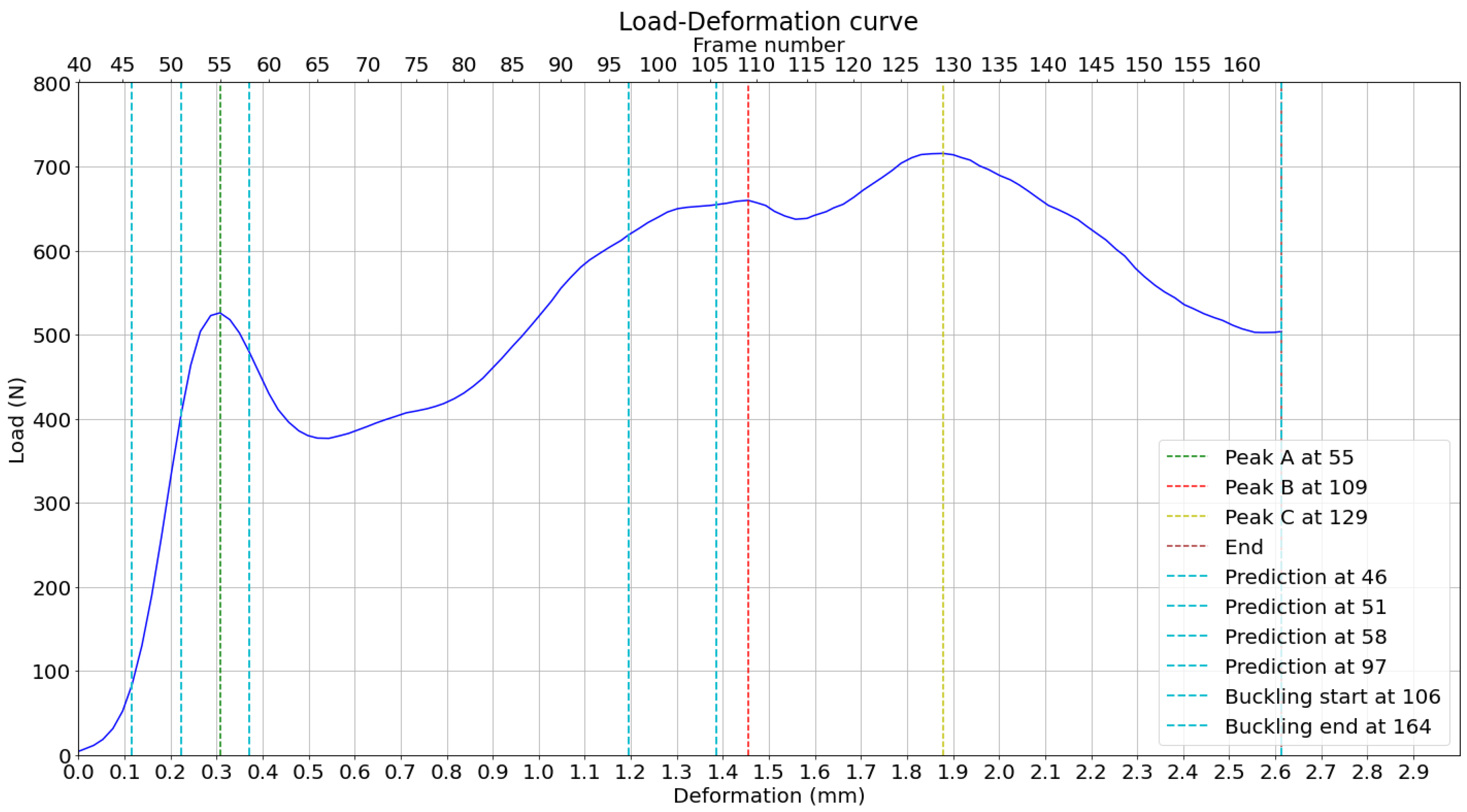
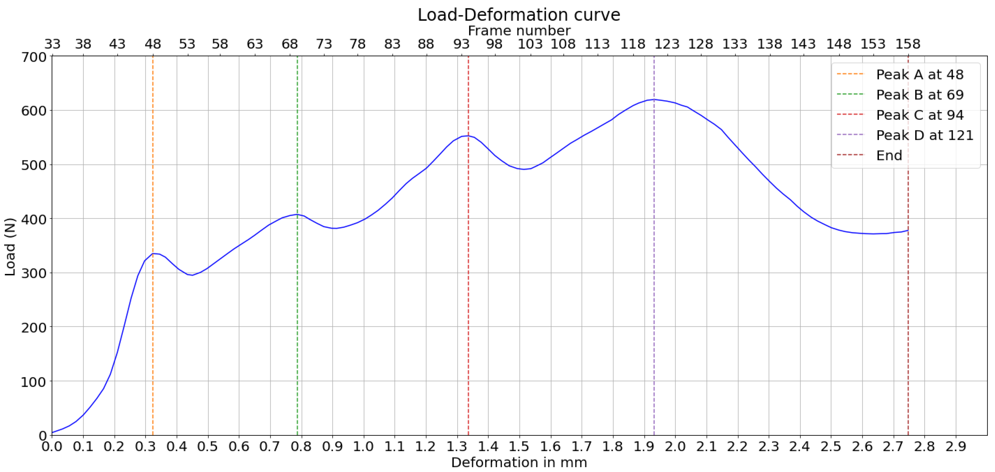
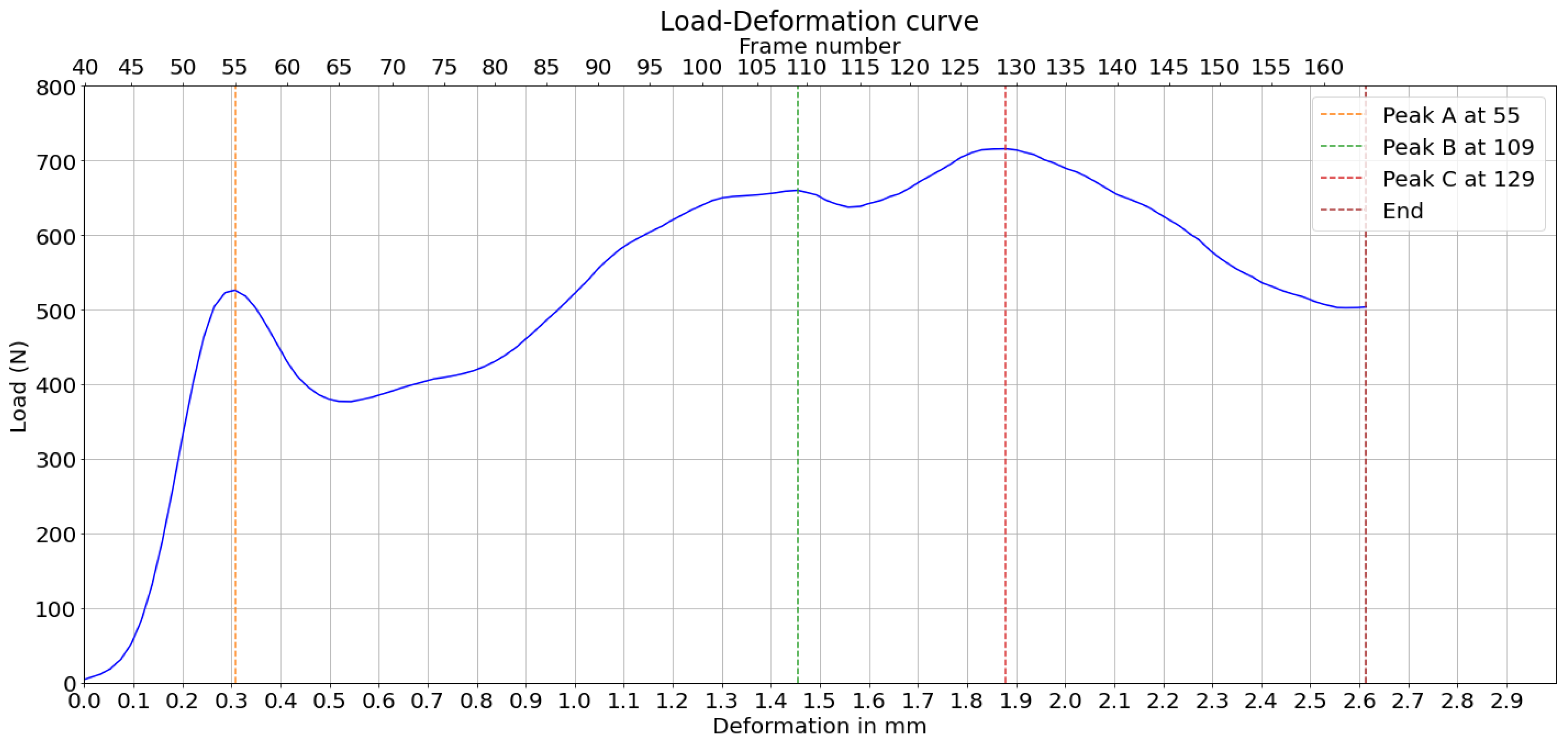
Two corrugated board specimens were selected based on the quality of the cross-section, which showed less delaminated paper fibers, and the clarity of the compression video. These two examples demonstrate the feasibility of graph-based image analysis in corrugated boards under compression. Their load-deformation curve are represented in Figure 5 and Figure 6. The load peaks are marked for later analysis. Geometric dimensions and characteristics are summarized in Table 1, where H and

λ

are the height of the board, respectively, as illustrated in Figure 4,

t_{f}

is the thickness of the flute paper and

t_{l}

is the thickness of the liner paper.

3.4. Filtering Process

The main goal of the filtering process illustrated in Figure 7 is to eliminate paper fibers mostly coming from the damages of paper sheets when cutting the samples and appearing on the corrugated board cross-section image. Furthermore, the process aims at smoothing the board geometry and converting the image to binary, without altering the structure of the board. The process consists of a Gaussian blurring followed by a binarization based on a constant threshold. Subsequently, a connected component filtering is applied to remove isolated white regions with an area smaller than a given value in pixels. Finally, median blurring is used to smooth the surface geometry of the corrugated board.

The filtering constants and kernel sizes are set manually and must be adapted to other samples individually to obtain optimal results. These manual adjustments of the filters depend on the thickness of the paper sheets constituting the different layers, the amount of delaminated paper fibers appearing on the cross-section image and the given light conditions. Default filters’ parameters are the following:

Gaussian filter: Kernel size set to 5x5 and sigma to 1.
Binarization Threshold set to 25.
Median filter: Kernel size set to 3x3.
Filter by connected components: Minimum size of white regions set to 150 pixels.

A morphological closing filter is replaced by a median blurring at the end, which not only fills the small black regions in a white surrounding but also smooths the surfaces and limits of the board. Histogram equalizer and adaptive Optimal Threshold Selection Using Otsu’s Method (OTSU) thresholding were investigated but did not help improve the image quality.

3.5. Skeletonization and Graph Building

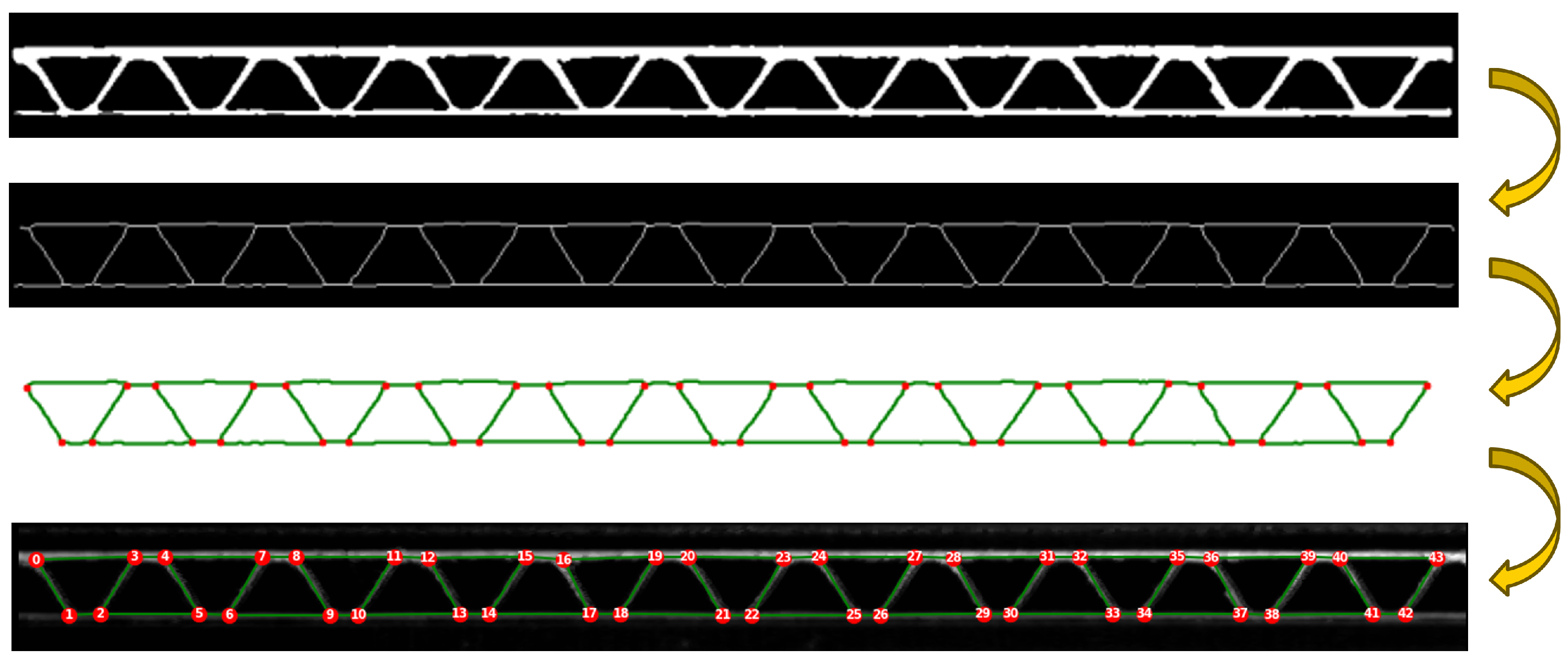
The skeletonization applied on the images of the corrugated board can be done by two different morphology functions from the Python library “Scikit-image". Function names are “skeletonize" and “thin." They use different algorithms to obtain skeletons of objects illustrated on binary images. The results of these two functions are slightly different. In Figure 8, one can observe that the curves of the sine wave are more preserved when the second function is used. Graphs are then built based on the obtained skeleton structure using the function “build_sknw" from the Python library “sknw" [20] with the following inputs:

multi: False, does not return a multigraph.
iso: False, does not return one-pixel node.
ring: False, does not return self-loops, i.e., edges of the form $(u, u)$ .
full: True, every edge starts from the nodes’ centroid.

This function builds a graph, which is a Networkx object, based on a skeleton structure. “Networkx" is a Python library used to create and analyze graphs. Skeleton branches represent graph edges, and intersections between branches are the graph nodes. Intersections between branches in a skeleton structure are constituted of three pixels or more. One pixel, which is the centroid, is set as a node representing the intersection. When the parameter full is set to True, edges are related to the centroid of every intersection. Results of both skeletonization and graph building are also illustrated in Figure 8.

There are two ways to visualize the graphs obtained: Using the skeleton branches as a visualization of edges, or using straight lines relating between the nodes, as illustrated in Figure 8 (lowest two sub-images). Graphs are mostly visualized using nodes and straight-line edges.

3.6. Graph Filtering and Node Tracking

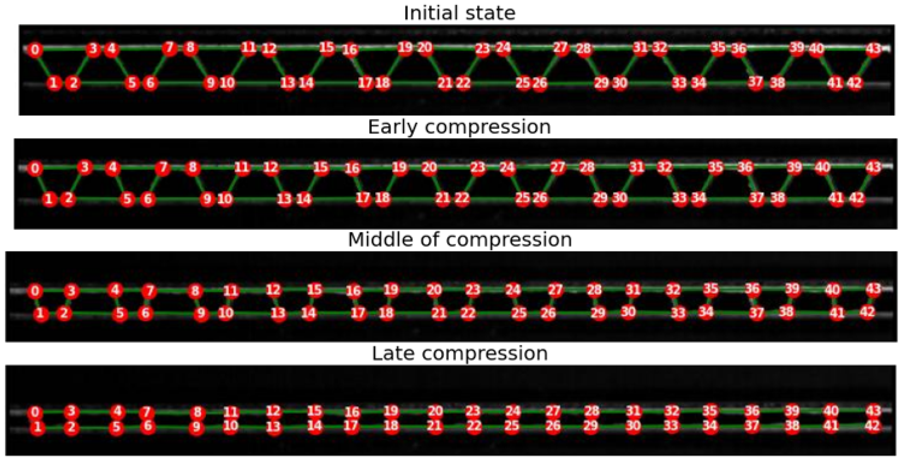
A simple first graph filtering is applied to every frame, and it is now described. An iteration is done to delete all nodes with a degree equal to one, which means that they are related to only one other node. These nodes represent either small paper fibers, which are not part of the structure, or endpoints of the graph at the left and right limits of the board, which are negligible in this work. For node tracking, the graph obtained from the first frame is taken as a reference. To ensure reasonable results of segmentation and tracking, the reference graph created from the first frame should depict the geometry of the corrugated board profile correctly. In the case of the used specimen, the first graph created indeed builds a correct geometry of the profile. The nodes of the first graph are relabeled and numbered from the left to the right of the board to make the tracking visualization easier.

For node tracking, an iteration over all the nodes in the graphs of every two successive frames is done, where the distances between one node of the subsequent graph and all the nodes of the previous one are calculated. The minimum distance corresponds to the closest node from the previous graph. Nodes having a minimum distance are associated with each other, if not already associated.

During the compression test, the deformation happening can influence the images and, consequently, the results of filtering, skeletonization, and graph-building. This can change the total number of nodes detected and the values of edges. In some frames, some nodes and edges cannot be detected, and in other frames, additional nodes and edges can emerge. When the number of nodes and the edge relations between them are not conserved, tracking problems can easily occur. Conserving the edge relations and the number of nodes along the frames of the compression video is necessary for the consistency of node tracking. A solution for this issue, which happens very often from frame to frame and especially when the nodes are very close to each other in the last frames corresponding to the end of the compression test, is suggested in the following four steps:

Nodes that are unique to the subsequent graph, i.e., additional nodes that emerge in the subsequent graph but were absent in the previous one, are eliminated because they are likely erroneous. This guarantees that the total number of nodes does not increase.
Nodes unique to the previous graph and not appearing in the subsequent graph are added in the same position. This ensures that the total number of nodes does not decrease.
All edges that are unique to the subsequent graph, i.e., edges that did not exist in the previous graph, are eliminated to prevent the formation of new relations between nodes, which would otherwise compromise the structure.
Edges unique to the previous graph, i.e., edges that correctly existed in the previous graph and are now absent in the subsequent graph, are added to ensure the structure is not missing any segments.

Results of the node tracking in some frames of the compression video are illustrated in Figure 9.

4. Results and Discussion

Even though more than two specimens were compressed, the authors are now presenting the analysis of the insights given by two of those experiments. Each experiment corresponds to each specimen. In the future, more experiments from more specimen compressions will also be analyzed and published online. Please check the data availability statement for more information. Moreover, this section attempts to answer the research questions and discuss the limitations.

4.1. Image and Graph Analysis: Experiment 1

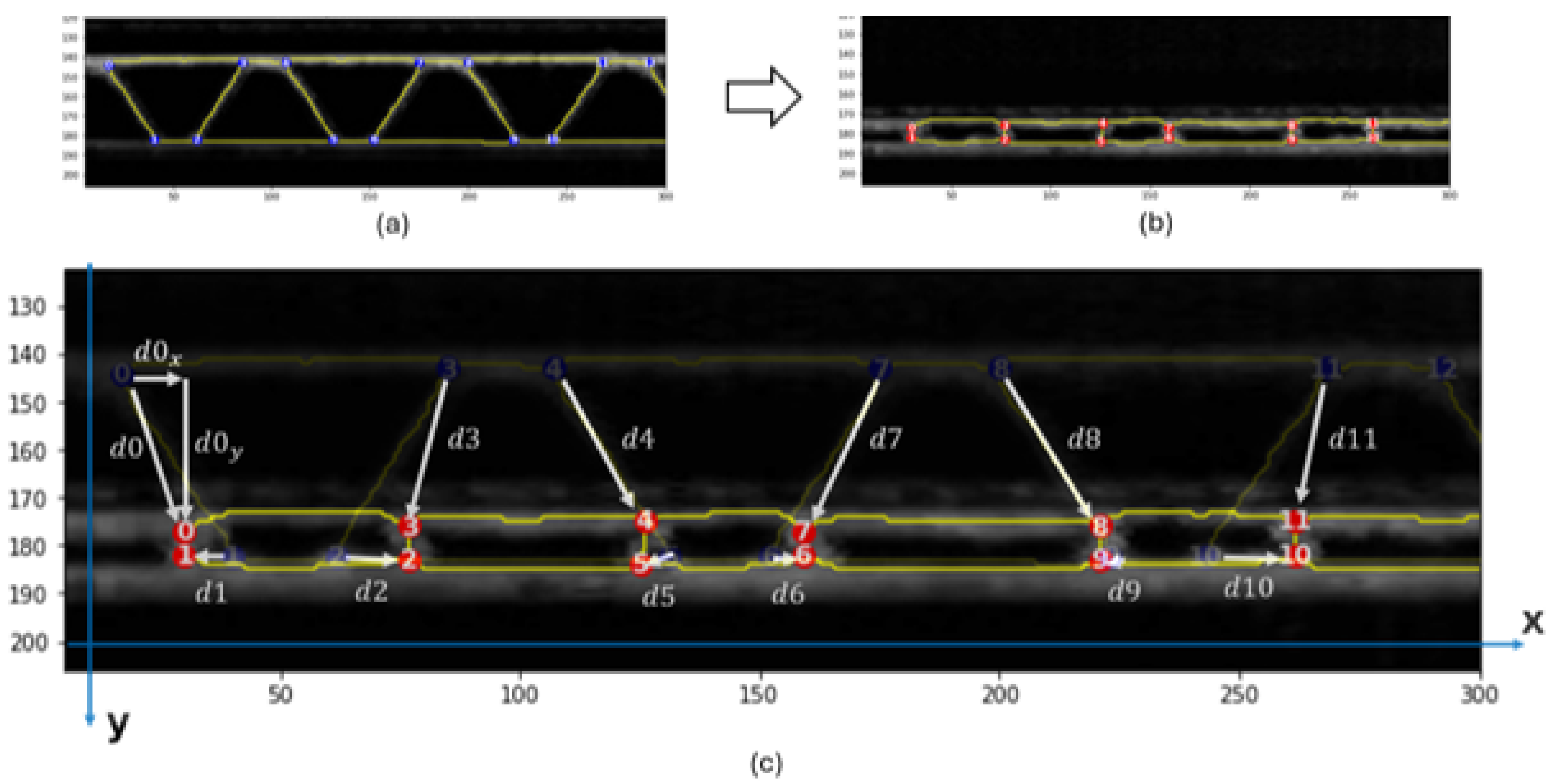
In the specimen used for this experiment, 44 nodes numbered from 0 to 43 are detected and tracked over the frames of the compression video. The displacement computation of every node is calculated and referenced to its position in frame 33, where the compression starts. To visualize the displacement of nodes, displacement vectors are manually drawn in Figure 10 for the nodes 0 to 11 between two frames extracted at the beginning and end of compression. The displacement computation of one node consists of calculating the magnitude of the displacement vector in every frame. It is also possible to calculate the magnitude of the horizontal component and the vertical component of the displacement vector separately, as illustrated for node 0.

d 0_{x}

represents the horizontal displacement of node zero and

d 0_{y}

represents its vertical displacement between these two frames. This way, curves of the horizontal and vertical displacements can be obtained and observed separately. Based on this, both vertical and horizontal displacements of all 44 nodes are calculated over all the frames.

Firstly, the vertical displacements are analyzed. The dendrogram of displacements at frame 157 (already at the end of the compression), as shown in Figure 11, provides evidence for the existence of two principal clusters of nodes (C1 and C2). An examination of the original dataset of node displacements and visualization of node groups and subgroups in the same figure reveals that the two main clusters align with the two expected groups of nodes perfectly, as cluster C1 contains all 22 nodes within the lower liner and all 22 nodes within the upper liner.

A second clustering method is based on the analysis of the horizontal displacements, whose resulting dendrogram is represented in Figure 12. Here, two main clusters can be separated. Cluster C2 contains the nodes on the right side in each pair, and a second main cluster, C1, contains the nodes on the left side in each pair.

The final two clustering methods, based on the horizontal and vertical displacements, provide two approaches to accurately forming two groups of nodes. The combination of these two methods, by creating sets of nodes based on the intersection of every 2 clusters, allowed for the creation of four distinct subgroups of nodes, as illustrated in Figure 13.

S u b g r o u p_{1} = C 1_{y} \cap C 2_{x} S u b g r o u p_{2} = C 1_{y} \cap C 1_{x}

S u b g r o u p_{3} = C 1_{y} \cap C 2_{x} S u b g r o u p_{4} = C 2_{y} \cap C 1_{x}

This way, all the nodes located periodically at the same position, labeled with top-left, top-right, bottom-left, and bottom-right, are separated into one subgroup. The formation of these four subgroups based on clustering the displacement curves shows that the nodes in every group experience similar displacements, which can be explained by the periodicity of the fluting medium. The nodes can be classified into two groups and four subgroups based on the different representations of displacements, i.e., absolute (or Euclidean), horizontal, and vertical displacements.

Based on the last four subgroups, displacement averages are calculated for every subgroup, as illustrated in Figure 14. Additionally, the four load peaks are indicated in the corresponding frame position.

One can observe that the average displacement curves of groups 1 and 4, corresponding to the nodes over the upper liner, start developing from the beginning of the compression phase, while groups 2 and 3, corresponding to nodes over the lower liner, start developing later, nearly at the same time as the load peaks are measured. The localized buckling of fluting segments causes the flattening of the fluting tips in contact with the lower liner, which is characterized by the displacement of nodes on this liner. However, there are no clear features that characterize the peaks A and D based on the displacement curves. The start of the movement can be detected by a displacement threshold of the average displacement curves of different groups set at 1,5 pixels.

Moreover, it is possible to observe from peak B that bottom-left nodes and bottom-right nodes have different Euclidean displacements. This means that the deformation does not happen symmetrically. While this is expected due to the geometric imperfections, this adds some relevant information that cannot be concluded based solely on the load-deformation curve.

The same can be applied based on the horizontal displacements of nodes. First, averages of horizontal displacements of different groups are calculated. Then, thresholds of 1,5 and -1,5 pixels are set to detect the start of movement as illustrated in Figure 15.

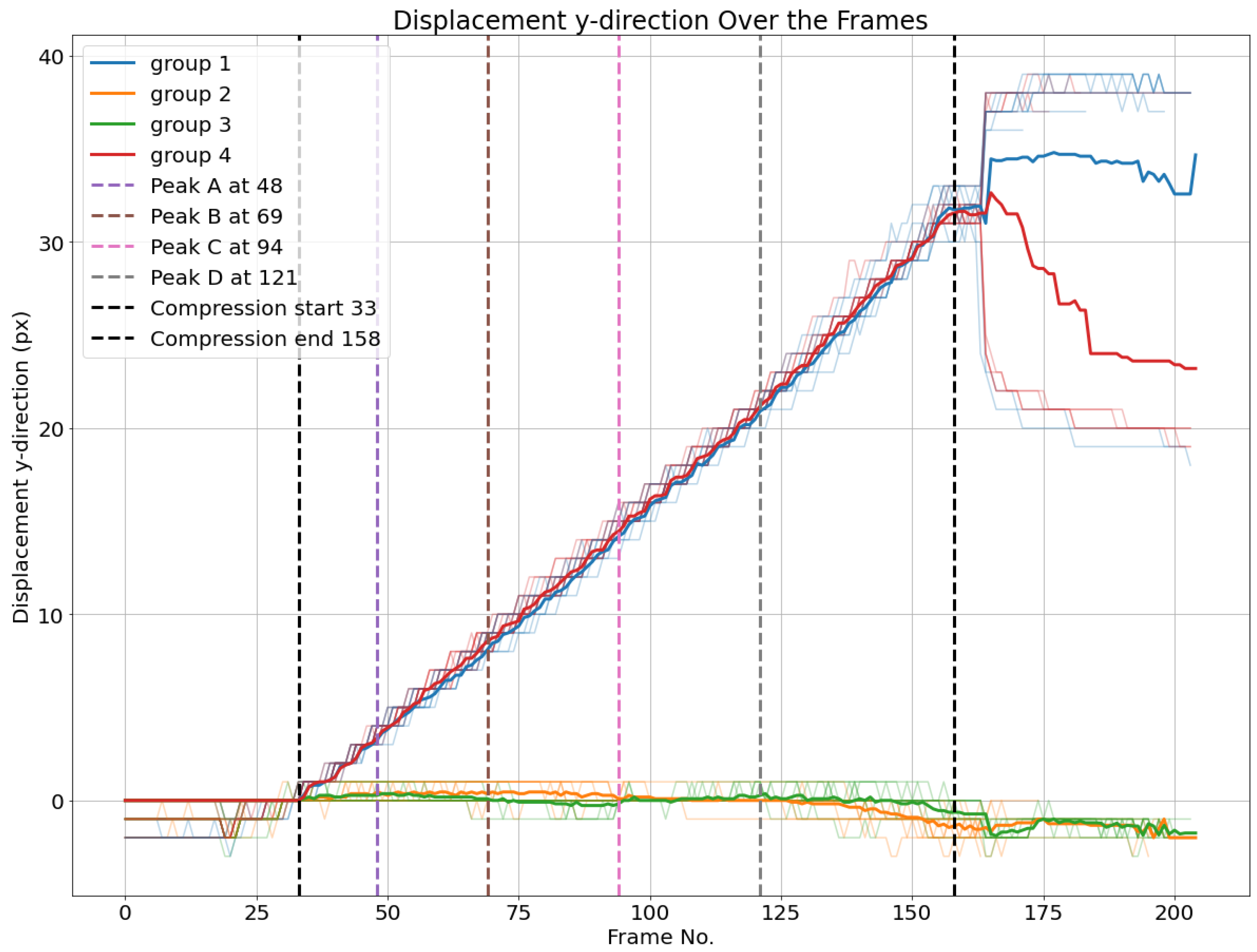
Additionally, the averaged vertical displacement for each of the four groups is illustrated in Figure 16. Groups 1 and 4, comprising nodes over the upper liner, have nearly identical vertical displacements in the compression phase. The same applies for the groups 2 and 3 of nodes over the lower liner, which have nearly no vertical displacement.

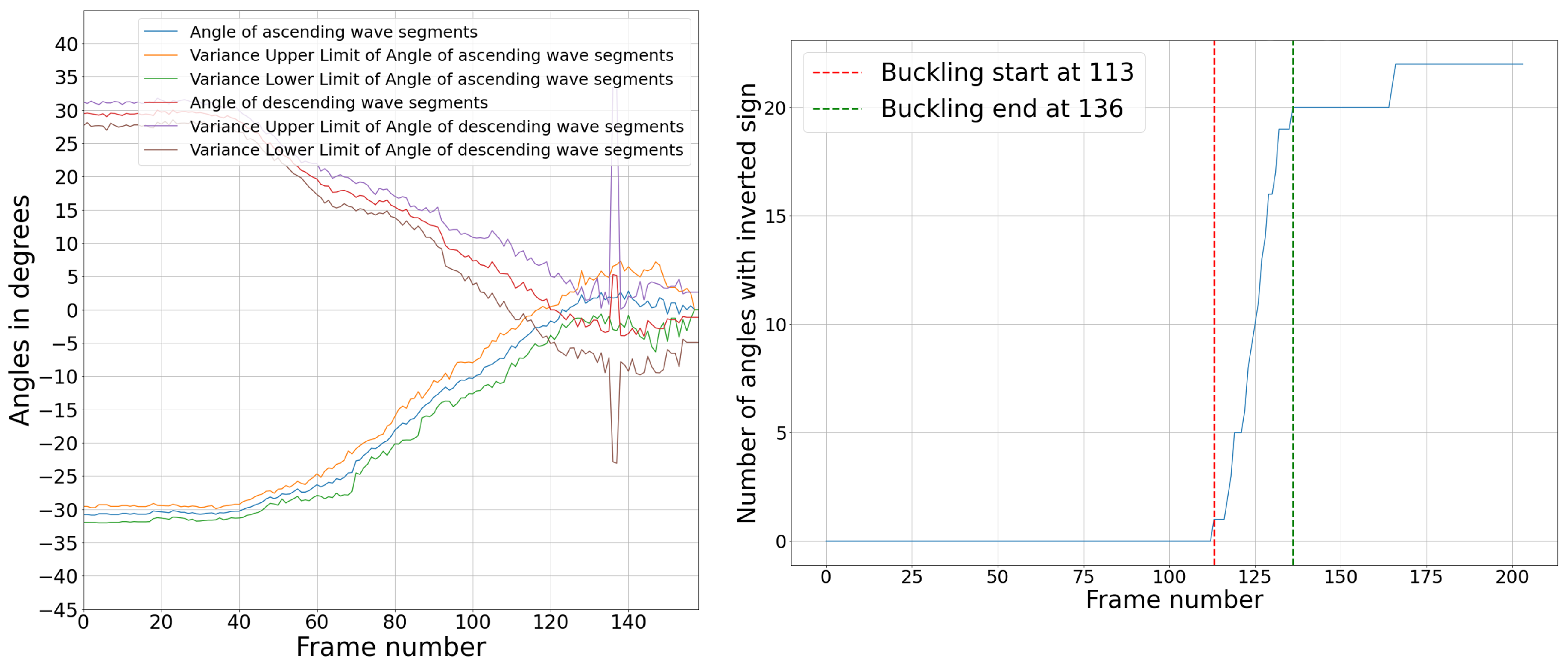
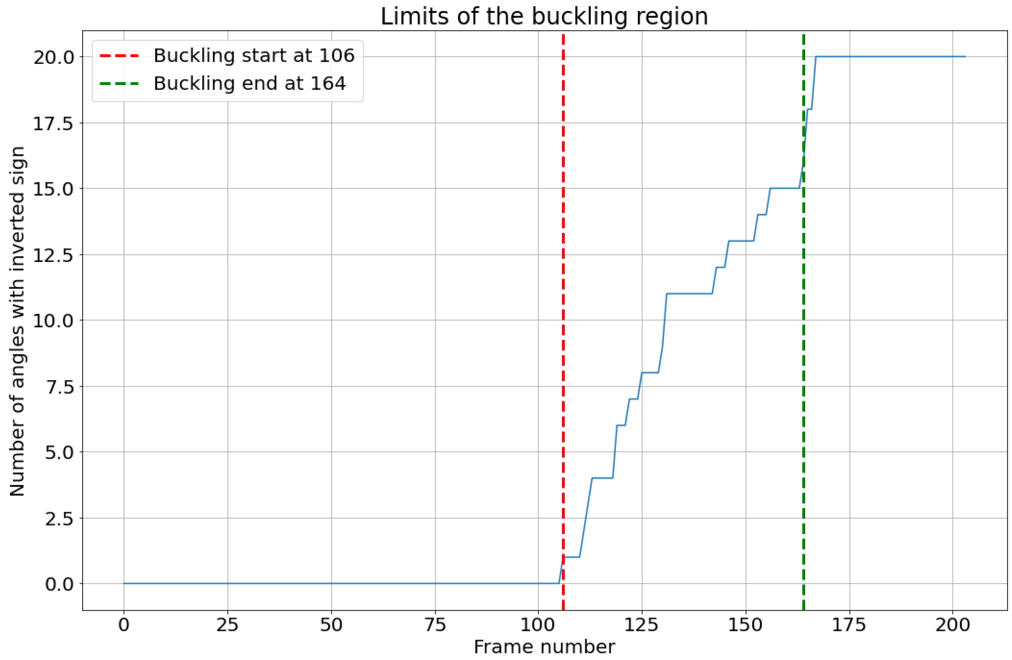
The highest load peak, D, was predicted in another approach based on the configuration of the board, which is characterized in this last peak by short vertical columns in the fluting medium. The load drop after this peak is caused by the buckling of the vertical fluting columns with an S-form. This causes the angles between the fluting column and the vertical axis in the TD to switch signs. The average angle values are first calculated and illustrated in Figure 17. At the beginning, as the fluting is sine-waved, angles have values around 30° and -30° with the vertical direction. This value changes towards zero during the compression as the fluting tips flatten and the middle fluting segments become more and more vertical. At a given point, they become totally vertical. That is where an angle equal to zero is measured. Most of the angles switch signs and then switch again. After this, the liners are very close to each other, and the fluting columns become too short, which causes errors in angle measurements. However, that is not relevant in this case, as the most important information to detect the peak position is the frames in which angles switch signs for the first time. The number of angles that switch signs in each frame is then calculated. Let us assume that when a fluting segment buckles, the angle with the vertical level switches signs. So, the buckling of the structure starts when the first segment switches its sign and ends when 90% of the total number of fluting segments switch signs. This range is illustrated in Figure 17.

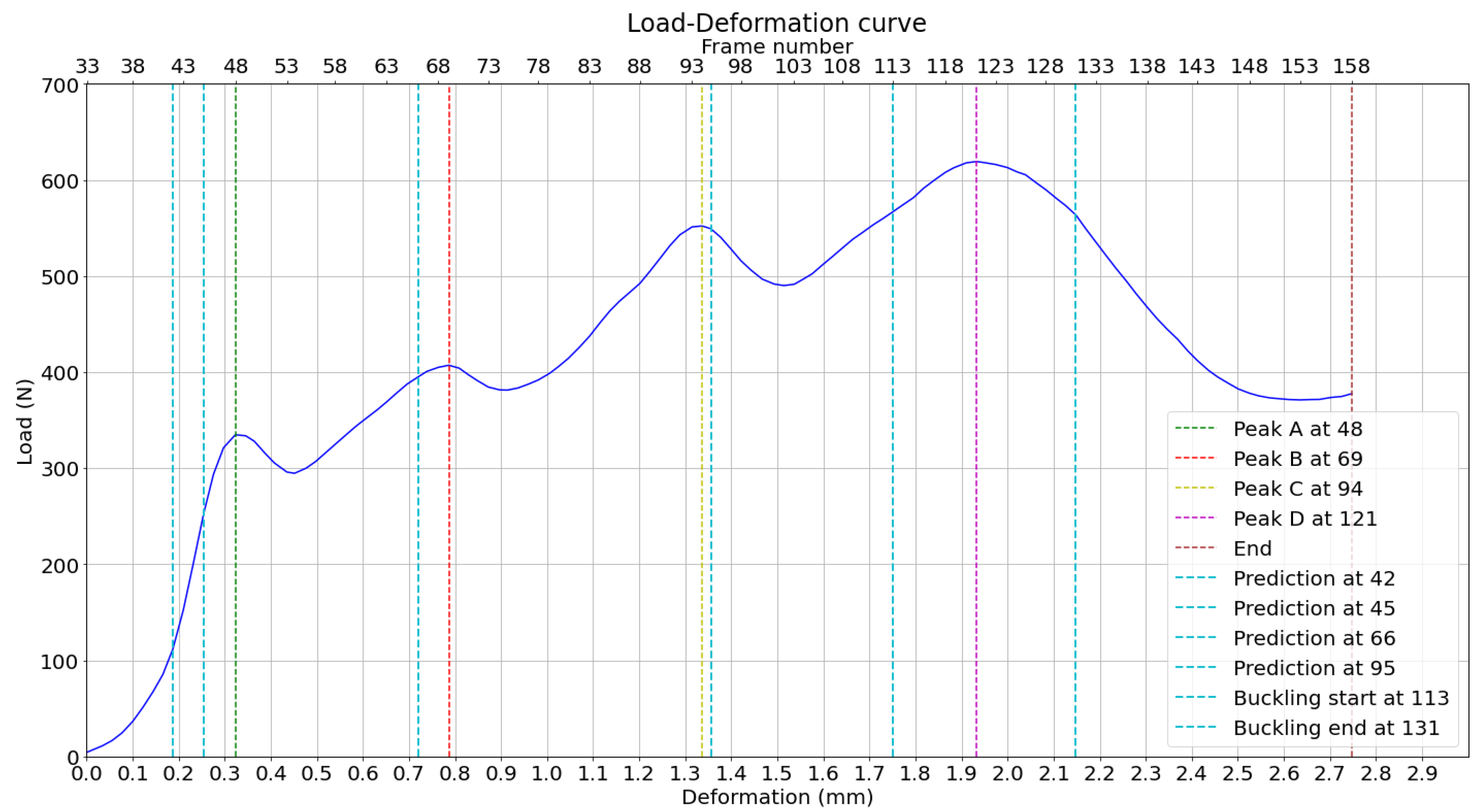
The measured peak loads and the positions of their predictions based on the displacement curves in the horizontal direction are then plotted on the load-deformation curve of the compression test, as shown in Figure 18. It can be observed, by direct observation of the bottom x-axis, that peaks A and B are predicted less than 100

μ m

of deformation before they happen. This attempt to predict the load peaks is based on averaged displacement curves, increasing reliability. The buckling range is around the highest peak, D, where the buckling is expected to happen.

4.2. Image and Graph Analysis: Experiment 2

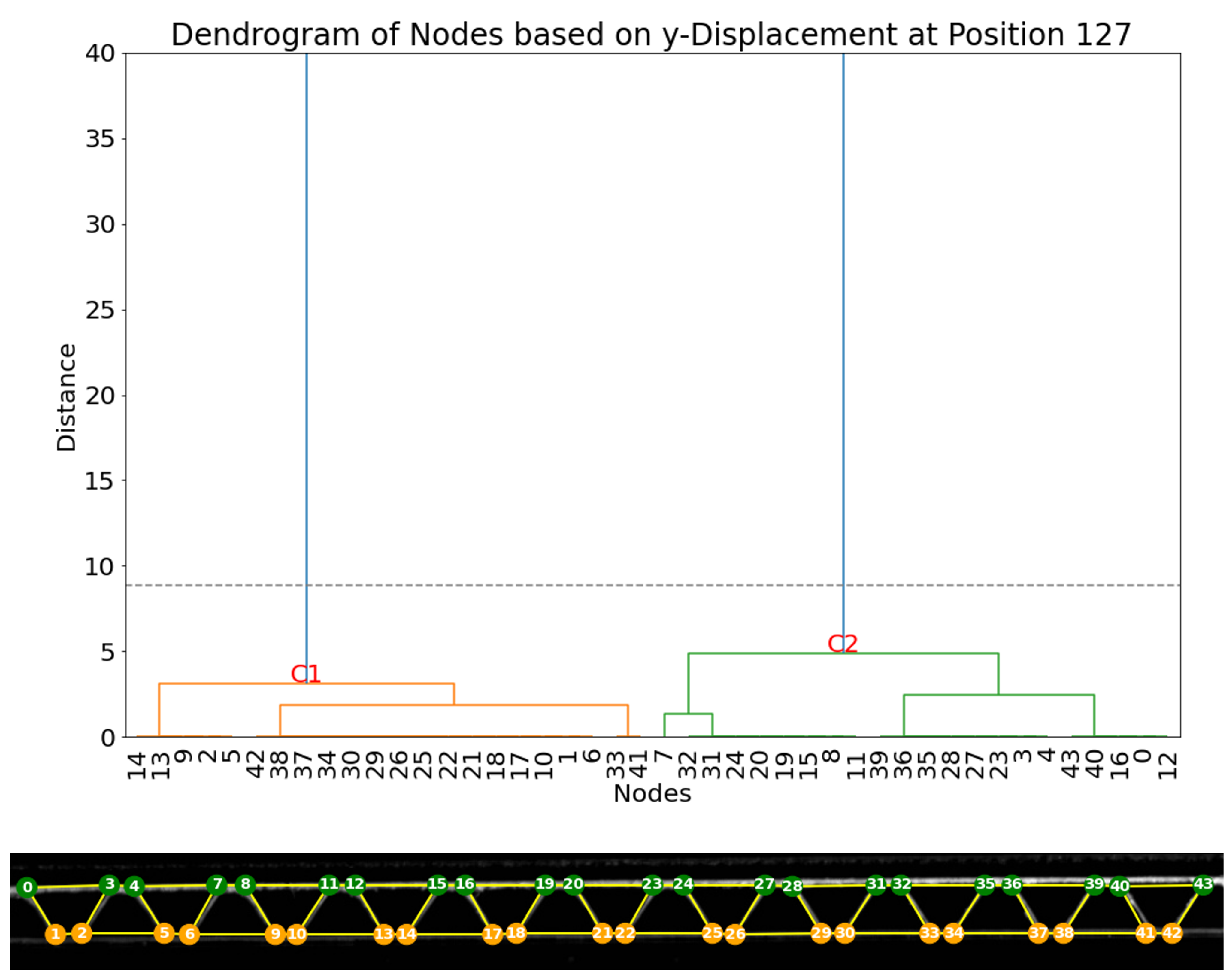
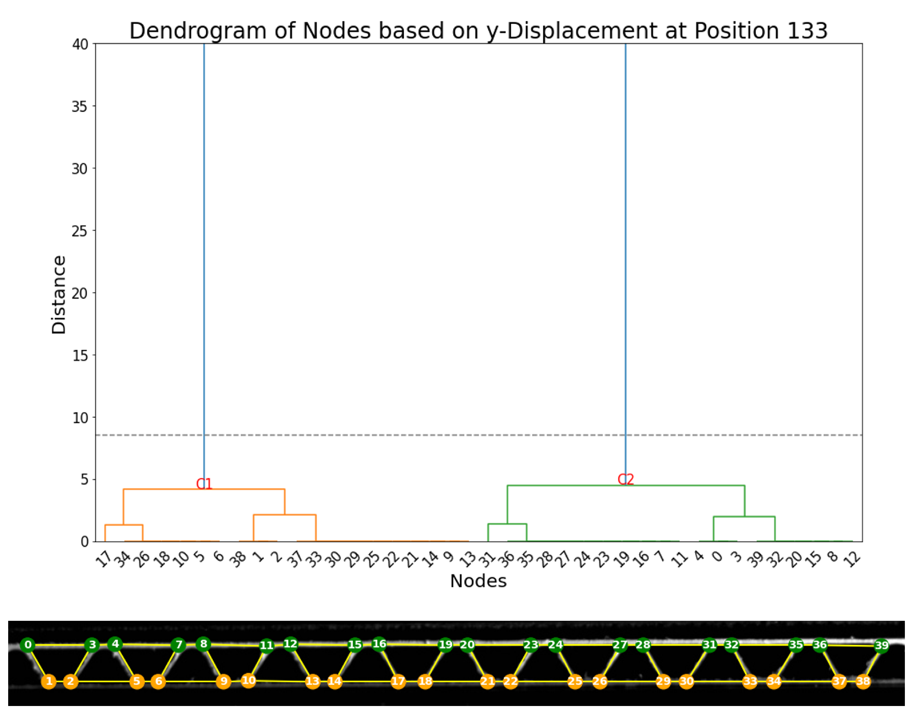
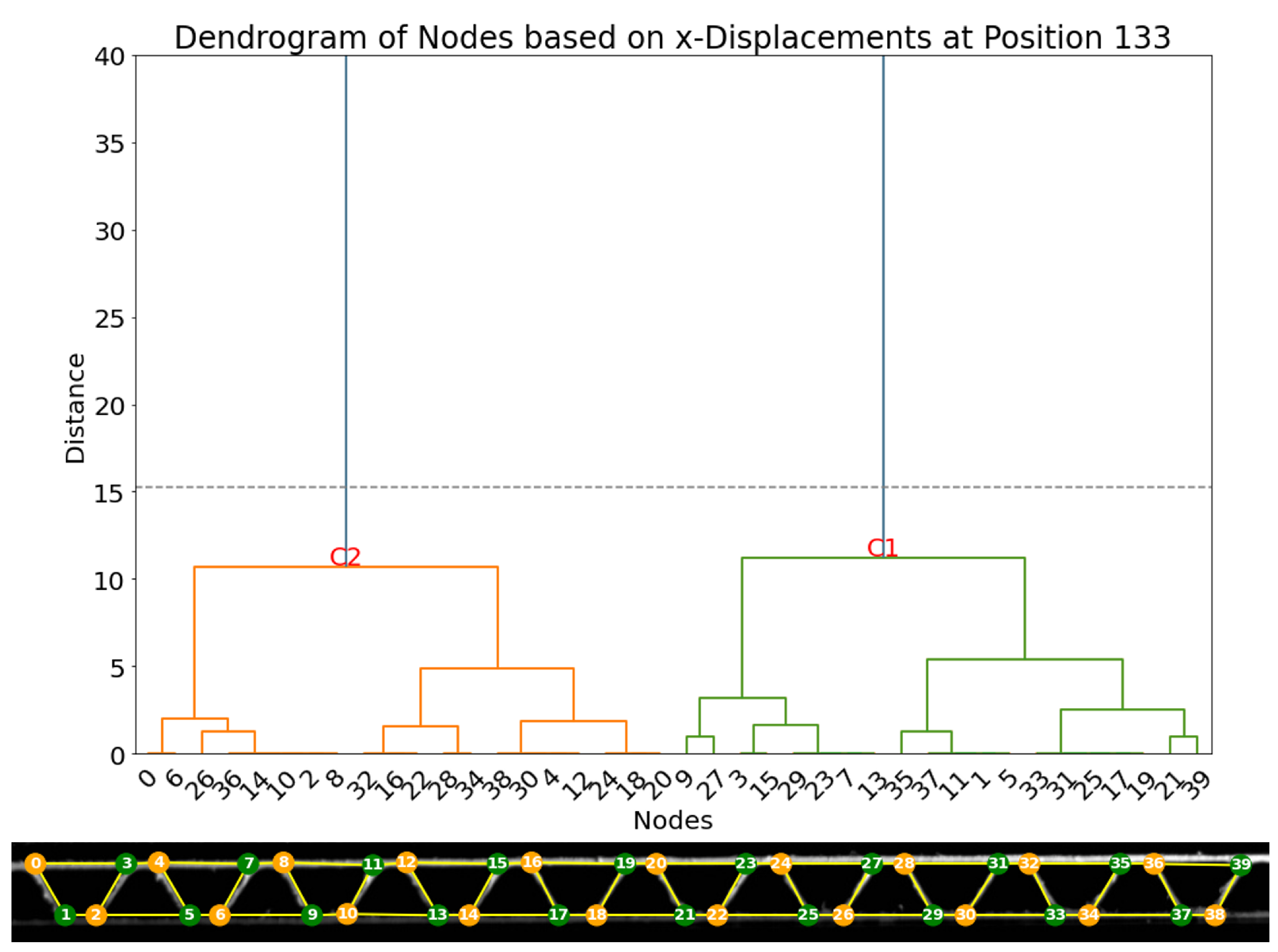
In this new specimen (Figure 19), 40 nodes were detected and tracked over the frames of the compression video. Firstly, the vertical displacements are analyzed. The dendrogram of displacements at frame 127, as shown in Figure 20, provides evidence for the existence of two principal clusters of nodes (C1 and C2). As observed in the first experiment, two main clusters align with the two expected groups of nodes perfectly, as cluster C1 contains all 20 nodes within the lower liner and all 20 nodes within the upper liner.

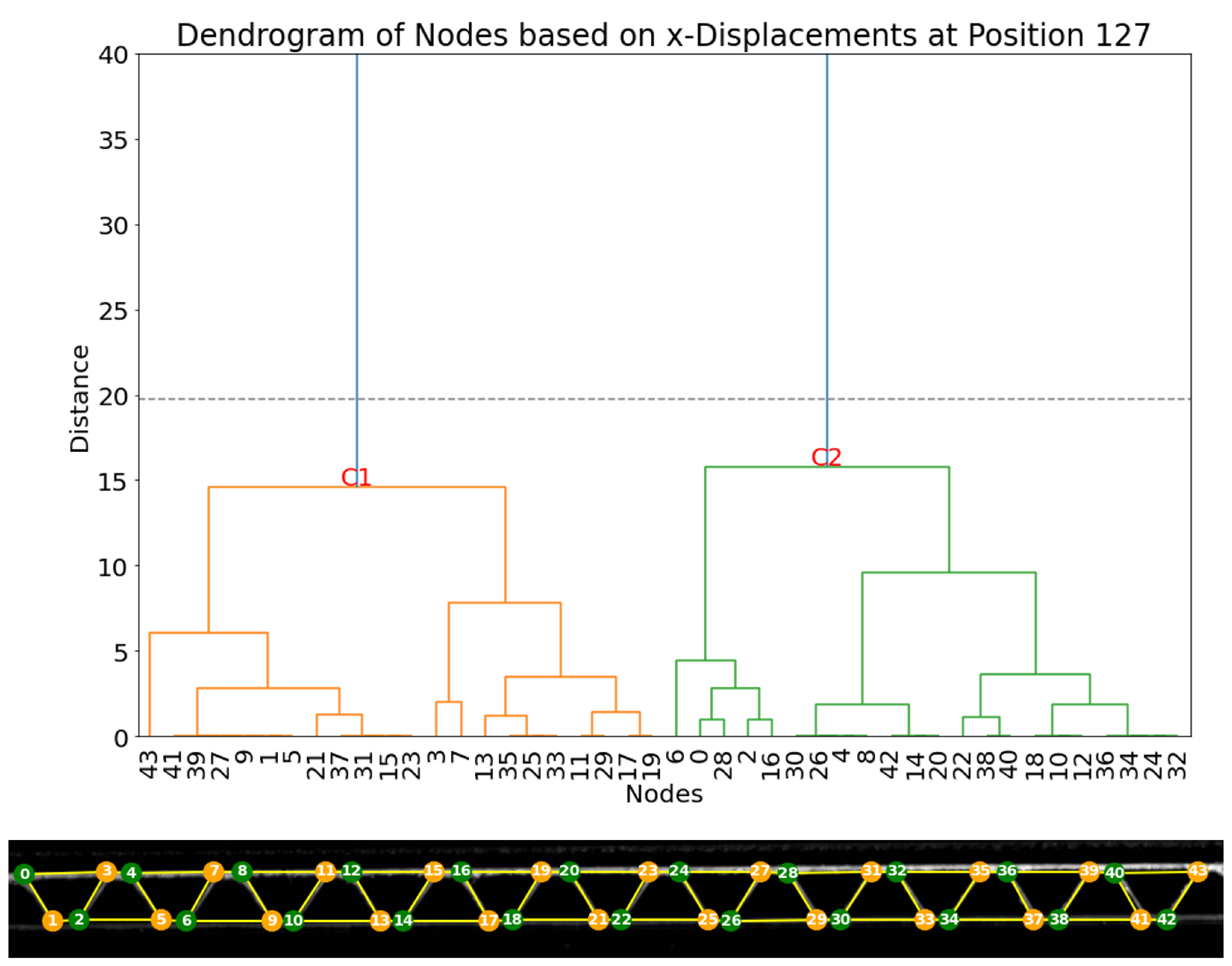
A second clustering method is based on the analysis of the horizontal displacements, whose resulting dendrogram is represented in Figure 21. Here, two main clusters can be separated in the same way as experiment 1.

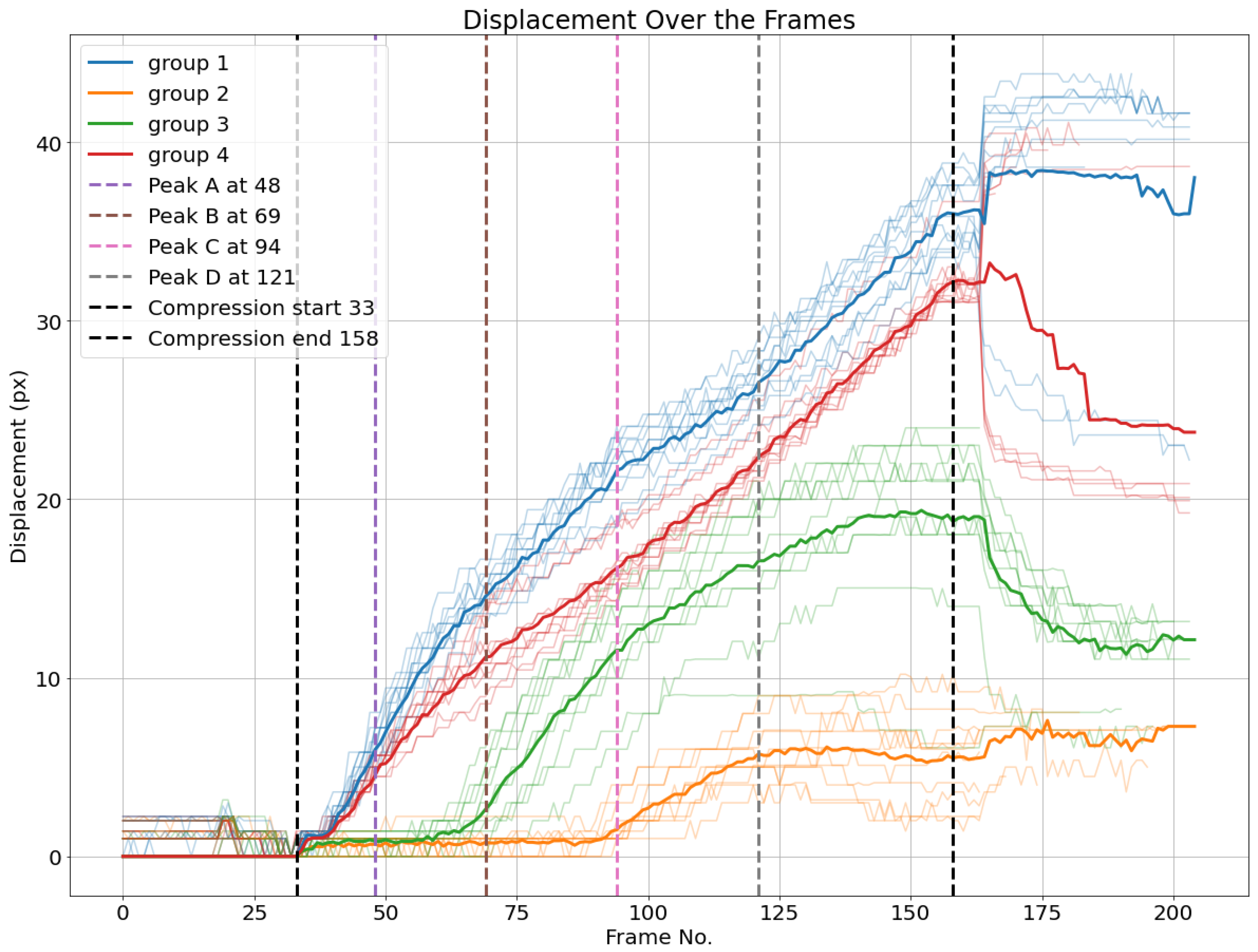
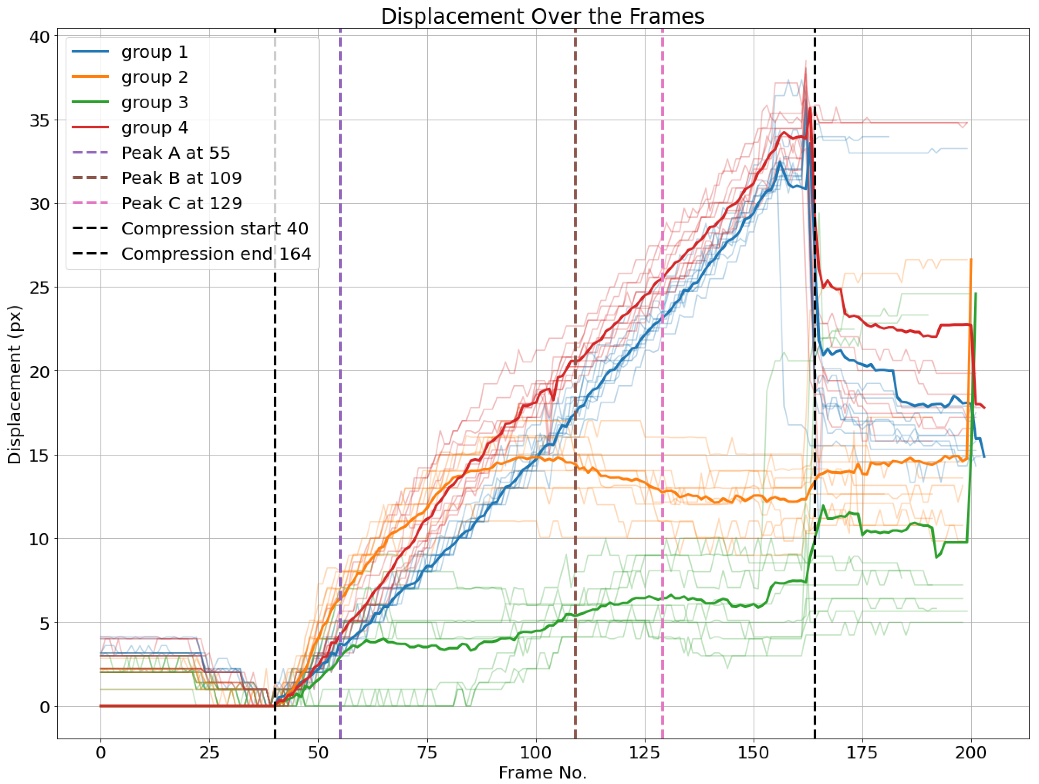
Based on the last four subgroups, displacement averages are calculated for every subgroup, as illustrated in Figure 23. Additionally, the four load peaks are indicated in the corresponding frame position.

One can observe that the average displacement curves of all groups start developing from the beginning of the compression phase, with groups 1 and 4, corresponding to the top liner, seeming not significantly different from each other in this perspective, and with the orange group (group 2) having a significant displacement, likely all of it corresponding to the horizontal displacement, as bottom liner nodes do not move vertically. This may suggest a significant move of the board to the left at the beginning of the compression, which is likely the way the structure becomes more stable for the rest of the compression.

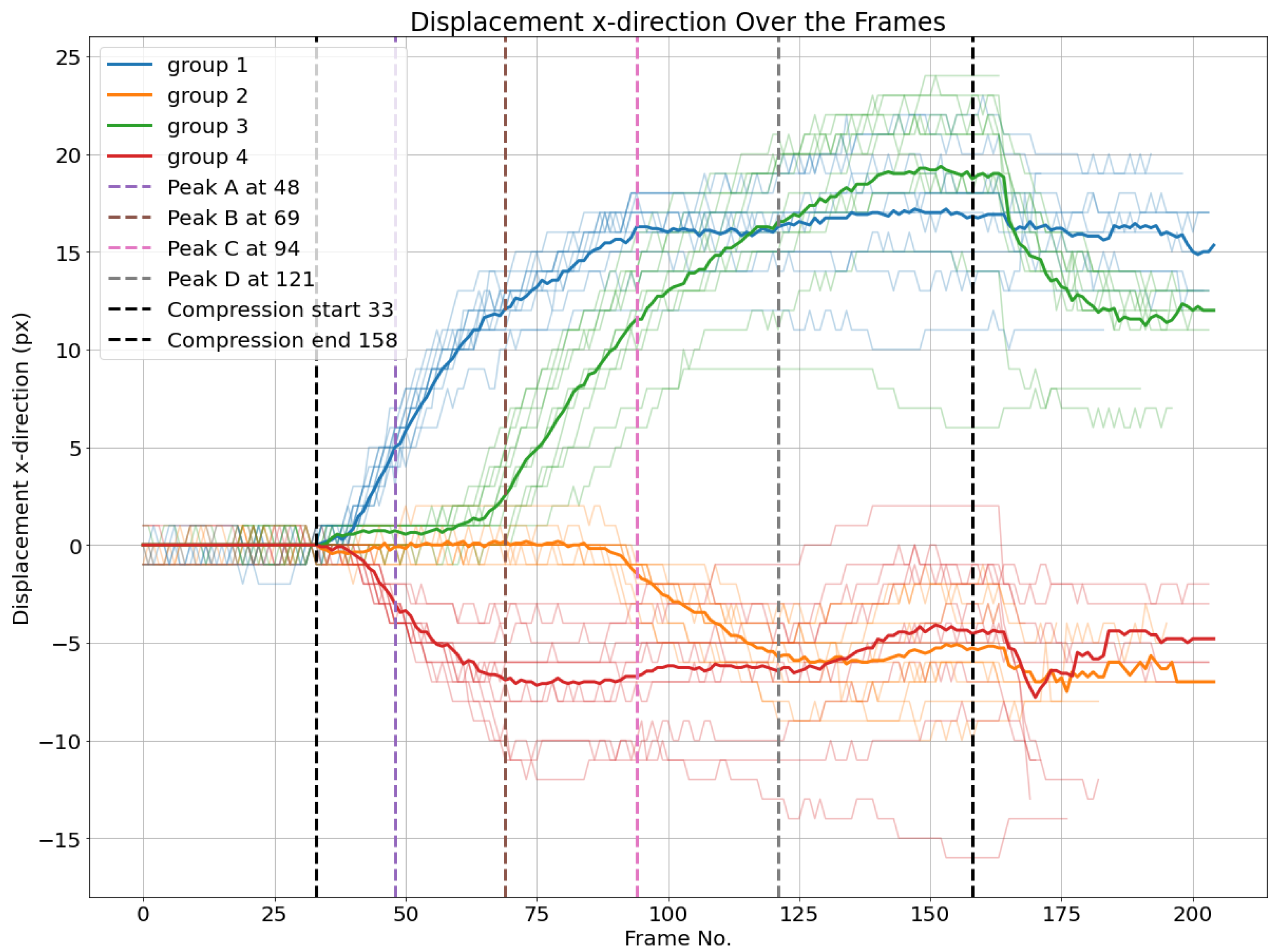
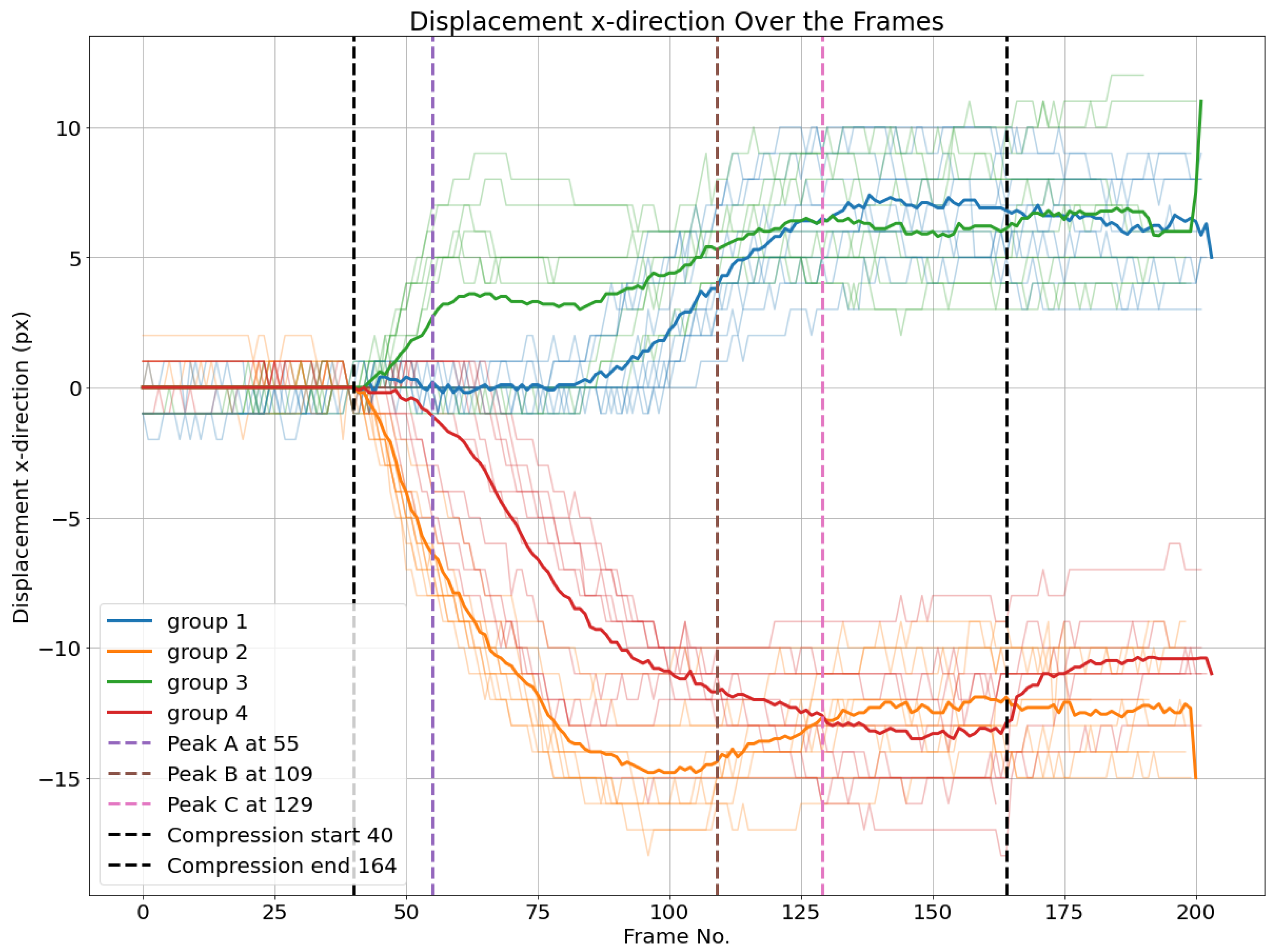
The same process is applied based on the horizontal displacements of nodes. First, averages of horizontal displacements of different groups are calculated. Then, thresholds of 1,5 and -1,5 pixels are set to detect the start of movement as illustrated in Figure 24.

While in experiment 1, it was possible to verify that upper liner nodes started to move horizontally first before the first peak compared to the nodes in the bottom liner, in experiment 2, it happened the opposite - in fact, bottom liner nodes were faster before the first peak, and then the top liner nodes. What is also interesting to observe is the fact that peak B happens after the last group to move horizontally, group 1. There is still another observation that is also possible to observe in Figure 24 in common with Figure 15 is that when the average of groups 1 and 3 intersect at the same time as groups 2 and 4, it also coincides with the last load-deformation curve peak. More experiments with different geometries may be necessary to explain it better.

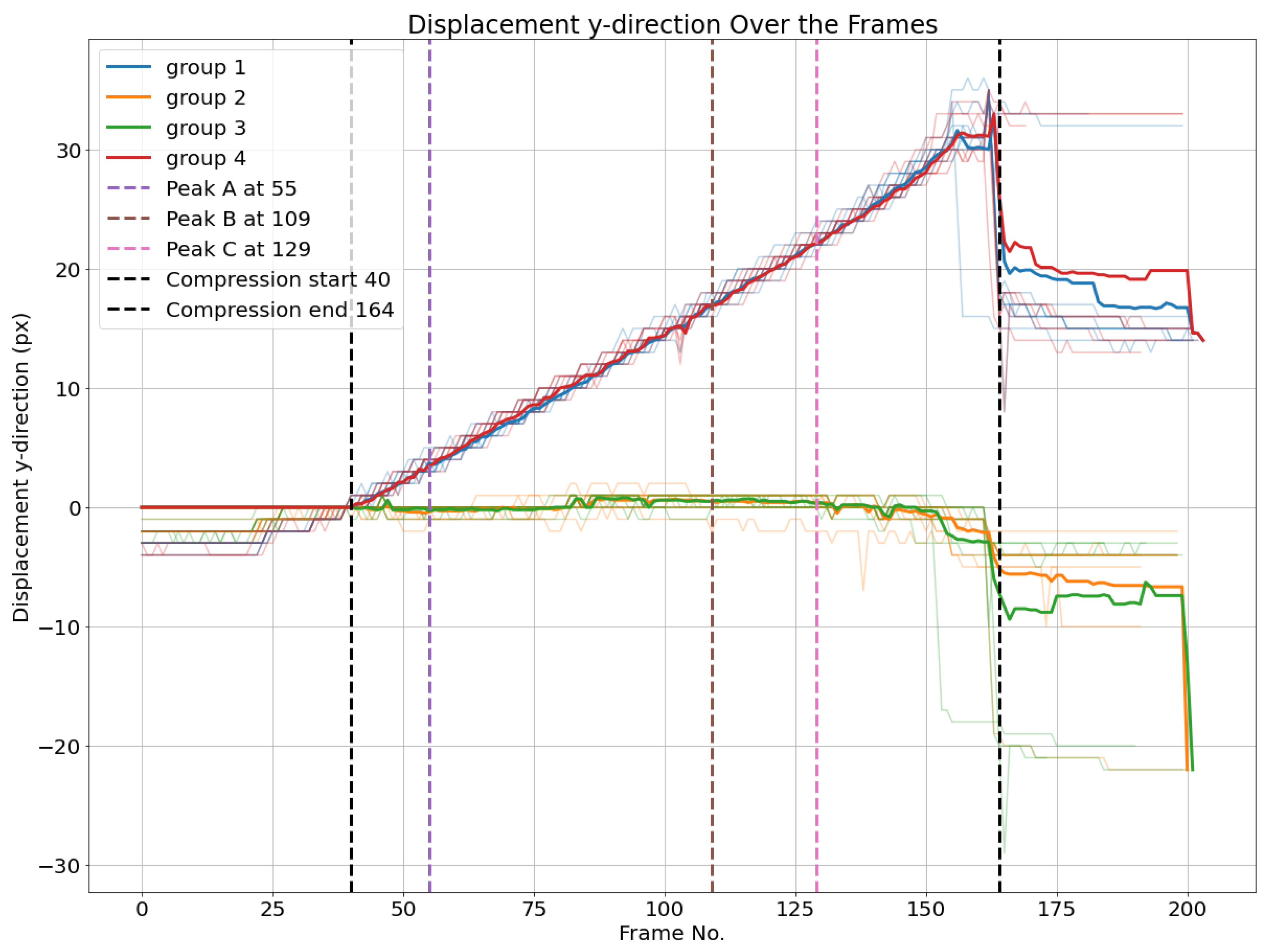
Additionally, the averaged vertical displacement for each of the four groups is illustrated in Figure 25. The behavior here identified is very similar to what had already been observed in experiment 1 (Figure 16).

As in experiment 1, the number of angles throughout the flute that switch signs in each frame is then calculated. Let us again assume that when a fluting segment buckles, the angle with the vertical level switches signs. So, the buckling of the structure starts when the first segment switches its sign and ends when 80% of the total number of fluting segments switch signs. This range is illustrated in Figure 26.

μ m

Figure 27. Load-deformation curve with measured and predicted load peaks, based on previous analysis.

4.3. Answering the Research Questions

Graphs proved to be advantageous to reduce the dimensionality of corrugated board images while preserving the most important information, which is the profile geometry during a compression test. Every frame of the videos recorded during the compression tests was replaced by a graph with a limited number of nodes and edges. This provided a reasonable amount of data that can be analyzed more efficiently than raw images. Although each image is approximately 44 KB in size, each graph objective requires only 4 KB, achieving a tenfold reduction in data size.

Moreover, the results showed that it is possible to collect multiple displacement curves from the nodes, and multiple clusters representing different compression behaviors could be analyzed. There is clearly a movement to one side that is firstly caused compared to the other, which is not seen in the load-deformation curve only. In the first experiment, the nodes moved to the right, while in the second experiment, the nodes moved to the left. This is important information that could be retrieved from the analysis made in the current study, as it can be useful for the prediction of the mechanical behavior, gaining more information than analyzing the load-deformation curve.

The following aspects were examined in both experiments:

The average of two out of the four sub-clusters started to make a significant horizontal displacement before the first peak happened;
The best reasonable predictors are observed using the horizontal displacement, but the vertical displacement is highly relevant for a different segmentation, allowing for the formation of the four sub-clusters;
All nodes have a significant displacement, in average, before buckling happens.

4.4. Limitations

The proposed procedure depends to a large extent on the image quality of the corrugated profile. However, the filtering input must be manually adapted for different samples to obtain optimal results. This can be improved and made more automatic by developing an adapted filtering process to eliminate the delaminated paper fibers. Automated and more robust filtering can improve the algorithm results and make it applicable to more samples with different qualities and imperfections. The experimental setup can be optimized so that videos are recorded under uniform light conditions. The profile geometry can be approximated more accurately by using more nodes and edges to describe the corrugated medium and better preserve the curvatures of the sine wave.

5. Conclusion

A graph-based image analysis of corrugated boards under compression is proposed as a new approach in this field to help understand the compressive behavior of corrugated boards based on their cross-section images. The profile geometry is approximated using graphs. Node tracking is implemented to associate nodes that represent the same regions in different frames with each other.

Based on a graph analysis consisting of the displacement computation of nodes, different groups of nodes could be clustered. The average displacement of each group is then calculated and used to predict the load peaks in the load-deformation curve corresponding to the buckling of the structure. The prediction of three load peaks out of four was relatively precise. Node displacements as a function of time provided new insights into the corrugated board deformation analysis. It is possible to observe when and in which regions of the board deformations are happening and buckling is spreading.

Improving the knowledge about the mechanical behavior of corrugated boards by a graph-based analysis and modeling of images of the real product could provide more opportunities for shape and topology optimizations, and the node application of graphs to approximate the profile geometry helped reduce the dimensionality of image data. This analysis with graphs can be also extended to other structures and other materials in future applications.

The limitations can be tackled in future work to improve the image analysis by developing an adapted filtering process and improving the precision of the geometry approximation by adapting the code and adding more nodes. Modeling can also be improved by a better approximation of the fluting geometry and by including the yield strength of paper sheets. This study represents the first application of graphs in the field of corrugated boards. Graphs can be useful in future research to apply machine learning techniques for the purpose of design optimization. It is also the reason why more experiments and more different geometries must be experimentally tested.

Moreover, replacing the graph with a beam structure model can allow for a rapid simulation of the board deformation under given load and boundary conditions. Regions where different stresses are maximized could then be identified. This should also be something to tackle in future works.s

Author Contributions

Conceptualization, T.B., R.F., HJ.S., and S.S.; methodology, T.B., R.F.; formal analysis, T.B.; investigation, T.B., R.F.; resources, R.F., HJ.S., and S.S.; writing—original draft preparation, T.B.; writing—review and editing, T.B., R.F., HJ.S., and S.S.; supervision, R.F., HJ.S., and S.S.; project administration, R.F., HJ.S. and S.S.; funding acquisition, HJ.S., and S.S. All authors have read and agreed to the published version of the manuscript.

Funding

Please add: “This research received no external funding” or “This research was funded by NAME OF FUNDER grant number XXX.” and and “The APC was funded by XXX”. Check carefully that the details given are accurate and use the standard spelling of funding agency names at https://search.crossref.org/funding, any errors may affect your future funding.

Data Availability Statement

The original data presented in the study are openly available in GitHub at https://github.com/ricardofitas/Graphs_Analysis_Corrugated_Boards.

Acknowledgments

This paper has been funded by the Technical University of Darmstadt through “OA-Fonds”, and it has been supported by the IGF Project Nr. 22371 N supported via AiF within the program for promoting the Industrial Collective Research (IGF) of the Federal Ministry of Economic Affairs and Climate Action (BMWK), based on a resolution of the German Parliament.

Conflicts of Interest

The authors declare no conflict of interest.

References

Fitas, R.; Schaffrath, H.J.; Schabel, S. A Review of Optimization for Corrugated Boards. Sustainability 2023, 15, 1–27. [Google Scholar] [CrossRef]
Nyman, U. Continuum mechanics modelling of corrugated board: Lund, Univ., Akad. avh., 2004; Vol. 04/1017, Structural Mechanics LUTVDG/TVSM, 2004.
Enlund, E.; Nilsson, J. Sustainable Decision-Making in the Fashion Industry : How to influence the fashion industry to adopt more sustainable packaging solutions. PhD thesis, 07.06.2021.
Jestratijevic, I.; Vrabič-Brodnjak, U. Sustainable and Innovative Packaging Solutions in the Fashion Industry: Global Report. Sustainability 2022, 14, 13476. [Google Scholar] [CrossRef]
LU, T.J.; CHEN, C.; ZHU, G. Compressive Behaviour of Corrugated Board Panels. Journal of Composite Materials 2001, 35, 2098–2126. [Google Scholar] [CrossRef]
Park, J.M.; Sim, J.M.; Jung, H.M. Finite Element Simulation of the Flat Crush Behavior of Corrugated Packages. Applied Sciences 2021, 11, 7867. [Google Scholar] [CrossRef]
Qiao, L.; Zhang, L.; Chen, S. Dimensionality reduction with adaptive graph. Frontiers of Computer Science 2013, 7, 745–753. [Google Scholar] [CrossRef]
Mao, Q.; Wang, L.; Goodison, S.; Sun, Y. Dimensionality Reduction Via Graph Structure Learning. In Proceedings of the Proceedings of the 21th ACM SIGKDD International Conference on Knowledge Discovery and Data Mining, New York, NY, USA, 2015. [CrossRef]
Rogalka, M.; Grabski, J.K.; Garbowski, T. Identification of Geometric Features of the Corrugated Board Using Images and Genetic Algorithm. Sensors (Basel, Switzerland) 2023, 23. [Google Scholar] [CrossRef] [PubMed]
Rogalka, M.; Grabski, J.K.; Garbowski, T. Deciphering Double-Walled Corrugated Board Geometry Using Image Analysis and Genetic Algorithms. Sensors 2024, 24, 1772. [Google Scholar] [CrossRef] [PubMed]
Rogalka, M.; Grabski, J.K.; Garbowski, T. A Comparison of Two Artificial Intelligence Approaches for Corrugated Board Type Classification. In Proceedings of the The 4th International Electronic Conference on Applied Sciences, Basel Switzerland; p. 272. [CrossRef]
Cebeci, U.; Aslan, F.; Çelik, M.; Aydın, H. Developing a New Counting Approach for the Corrugated Boards and Its Industrial Application by Using Image Processing Algorithm. In Practical applications of intelligent systems; Wen, Z., Li, T., Eds.; Springer: Heidelberg and New York, NY and Dordrecht and London and Berlin, 2014; Vol. 279, Advances in Intelligent Systems and Computing; pp. 1021–1040. [Google Scholar] [CrossRef]
Suppitaksakul, C.; Suwannakit, W. A Combination of Corrugated Cardboard Images Using Image Stitching Technique. In Proceedings of the 2018 15th International Conference on Electrical Engineering/Electronics, Computer, Telecommunications and Information Technology (ECTI-CON). IEEE, 2018. [CrossRef]
Balestrino, A.; Landi, A.; Pacini, L. Vision system for monitoring the production of corrugated cardboard. In Proceedings of the 2006 IEEE Conference on Computer Aided Control System Design, 2006 IEEE International Conference on Control Applications, 2006 IEEE International Symposium on Intelligent Control. IEEE, 10/4/2006 - 10/6/2006, pp. 626–631. [CrossRef]
Radi, K.; Allamand, F.; Kochmann, D.M. Deformation tracking of truss lattices under dynamic loading based on Digital Image Correlation. Mechanics of Materials 2023, 183, 104658. [Google Scholar] [CrossRef]
Hu, X.; Wang, H.; Gu, J.; Zhang, A.; Hu, Y.; Tang, X. Deformation tracking of honeycomb structure based on image skeletonization and branch point matching. Optics and Lasers in Engineering 2025, 184, 108622. [Google Scholar] [CrossRef]
Liang, B.; Chaudet, P.; Boisse, P. Curvature determination in the bending test of continuous fibre reinforcements. Strain 2017, 53. [Google Scholar] [CrossRef]
Diestel, R. Graph theory, fifth edition, first softcover printing ed.; Vol. 173, Graduate Texts in Mathematics, Springer Nature: Berlin, 2018.
Noah, C.; Jenny, N. Introduction to graph theory.
yxdragon. GitHub - Image-Py/sknw: build net work from skeleton image (2D-3D), 18.08.2024.

Figure 1. Example of an undirected, connected, and simple graph.

Figure 2. Flowchart representing the methodology followed in the current paper.

Figure 3. Simple representation of the experimental setup.

Figure 4. Dimensions of the corrugated board sample: (a) 3D view; (b) 2D profile.

Figure 5. Load-deformation curve corresponding to the compression test being analyzed - Experiment 1.

Figure 6. Load-deformation curve corresponding to the compression test being analyzed - Experiment 2.

Figure 7. Filtering Process.

Figure 8. Process from Image to Graph.

Figure 9. Results of the node tracking.

Figure 10. Visualization of the Displacement vectors representing the displacement of the nodes between the initial (a) and final (b) frames. Displacement vectors are seen from nodes 1 to 11 (c).

Figure 11. Top: dendrogram and resulting clustering of the nodes based on vertical displacement in frame 127; Bottom: visualization of the clusters (cluster 1: orange; cluster 2: green).

Figure 12. Top: dendrogram and resulting clustering of the nodes based on horizontal displacement in frame 127; Bottom: visualization of the clusters (cluster 1: orange; cluster 2: green).

Figure 13. Visualization of the resulting four subgroups based on the combination of the pairs of subgroups resulting from the vertical and horizontal displacements.

Figure 14. Euclidean displacements of node groups. The average of each cluster per frame is plotted.

Figure 15. Horizontal displacements of node groups. The average of each cluster per frame is plotted.

Figure 16. Vertical displacements of node groups. The average of each cluster per frame is plotted.

Figure 17. Left: Angle variation over the frames, per node group; Right: Buckling analysis.

Figure 18. Load-deformaton curve with measured and predicted load peaks, based on previous analysis.

Figure 19. Graph visualization of the specimen of the second experiment.

Figure 20. Top: dendrogram and resulting clustering of the nodes based on vertical displacement in frame 133; Bottom: visualization of the clusters (cluster 1: orange; cluster 2: green).

Figure 21. Top: dendrogram and resulting clustering of the nodes based on horizontal displacement in frame 133; Bottom: visualization of the clusters (cluster 1: green; cluster 2: orange).

Figure 22. Visualization of the resulting four subgroups based on the combination of the pairs of subgroups resulting from the vertical and horizontal displacements.

Figure 23. Euclidean displacements of node groups. The average of each cluster per frame is plotted.

Figure 24. Horizontal displacements of node groups. The average of each cluster per frame is plotted.

Figure 25. Vertical displacements of node groups. The average of each cluster per frame is plotted.

Figure 26. Left: Angle variation over the frames, per node group; Right: Buckling analysis.

Table 1. Corrugated board samples dimensions.

Flute Type	H (mm)	$λ$ (mm)	$t_{f}$ ( $μ$ m)	$t_{l}$ ( $μ$ m)
C	4.0 ± 0.1	8.0 ± 0.2	250 ± 80	250 ± 80

Disclaimer/Publisher’s Note: The statements, opinions and data contained in all publications are solely those of the individual author(s) and contributor(s) and not of MDPI and/or the editor(s). MDPI and/or the editor(s) disclaim responsibility for any injury to people or property resulting from any ideas, methods, instructions or products referred to in the content.

© 2024 by the authors. Licensee MDPI, Basel, Switzerland. This article is an open access article distributed under the terms and conditions of the Creative Commons Attribution (CC BY) license (http://creativecommons.org/licenses/by/4.0/).

Copyright: This open access article is published under a Creative Commons CC BY 4.0 license, which permit the free download, distribution, and reuse, provided that the author and preprint are cited in any reuse.

Alerts

MDPI Initiatives

Important Links

Choose an area of interest and we will send you notifications of new preprints at your preferred frequency.

Disclaimer