
Submitted:
05 November 2024
Posted:
06 November 2024
You are already at the latest version
Abstract
This study introduces a novel method for optimising the size and control strategy of grid-connected, utility-scale photovoltaic (PV) systems with battery storage aimed at energy arbitrage and frequency containment reserve (FCR) services. By applying genetic algorithms (GA), the optimal configurations of PV generators, inverters/chargers, and batteries are determined, focusing on maximising the net present value (NPV). Both DC- and AC-coupled systems are explored. The performance of each configuration is simulated over a 25-year lifespan, considering varying pricing, solar resources, battery ageing, and PV degradation. Constraints include investment costs, capacity factors, and land use. A case study conducted in Wiesenthal, Germany, is followed by sensitivity analyses, revealing that a 75% reduction in battery costs is needed to make AC-coupled PV-plus-battery systems as profitable as PV-only systems. Further analysis shows that changes in electricity and FCR pricing, as well as limits on FCR charging, can significantly impact NPV. The study confirms that integrating arbitrage and FCR services can optimize system profitability.
Keywords:
Photovoltaic
; battery
; PV-plus-battery
; utility-scale
; battery degradation
; simulation and optimisation
1. Introduction
Utility-scale PV generators sell electricity to AC grids in the long-term market through a power purchase agreement (PPA) or in the daily/intraday market, thus establishing a marginal cost of electricity [1]. Adding storage to PV generators, specifically batteries (PV-plus-battery systems), helps the system enhance its functionality through energy arbitrage and a range of support services, including black start capability, frequency regulation, reactive support, voltage control, and strategic participation in ancillary service markets [2,3]. Other benefits can also be obtained using batteries, such as reduced curtailment or ramp rate control. Zhao et al. [4] reviewed the application and integration of grid-connected batteries.
Energy arbitrage consists of storing the energy produced by the PV generator (charging the battery) when the energy prices are low (usually when there is low demand) and selling it by discharging the battery when the prices are high (high demand).
FCR is an ancillary service, also known as the primary control reserve (PCR), which is the first response to frequency disturbances. When frequency deviations occur, FCR intervenes automatically within seconds to restore the balance between supply and demand. Battery systems are particularly suitable for FCR because of their short reaction times (less than 1 sec considering the total response time, including control and inverter delays) [5].
With the continuous increase in renewable energy generation, the shape of day-ahead hourly price curves has changed, lowering daytime prices [6]. When the PV penetration is high, the hourly electricity price turns into a “duck” shape [7], with significantly low prices at noontime (high photovoltaic generation), as it happened in California [6] and Western Australia [7]; in these cases, storage can be helpful to provide energy arbitrage and ancillary services such as FCR. Depending on the shape of the curve (the “duck” curve encourages storage in PV generators) and the battery cost and duration, energy arbitrage can be economically viable in PV-plus-battery systems compared to PV-only systems. Zhao et al. [6] showed the dependence of electricity market prices on renewable penetration and also on storage: with an increase in storage, it will no longer be a price-taker but also a price-maker, and concluded that with the expected cost reduction, Li-ion batteries would dominate the storage market (compared to lead–acid, vanadium redox flow batteries, and compressed air energy storage).
PV-plus-battery plants are economically viable in specific scenarios, such as improving flexibility and system performance [8]. In the literature review, previous studies analysed energy arbitrage using batteries. Many have found that storage costs should be reduced to be financially rewarding, but others have found it profitable. However, this depends on the storage costs, degradation, and hourly electricity pricing curves. The following paragraphs present the main contributions obtained in the literature review.
Zhang et al. [9] asserted that price arbitrage using only storage (charge from the grid at low prices and discharge at high prices) is not viable because storage capacity costs are high, specifically for Li-ion batteries. The authors of the current study found similar results [10]. Hu et al. [11] analysed energy arbitrage using battery energy storage systems (BESS) in European countries. Using a Li-ion battery as a reference, the wear cost was higher than 0.073 €/kWh and the hourly electricity price of the daily market in 2019 and 2020. They concluded that energy arbitrage with Li-ion batteries was only suitable for less than 10% of the time during those years. However, the PV-plus-battery system can be profitable at different spot prices, battery costs, and durations. Arcos-Vargas et al. [12] presented a mixed-integer linear programming (MILP) model for the optimisation of the battery and inverter size and a trading strategy for energy arbitrage of BESS in the Spanish electrical system, considering the recent reduction in costs and increase in roundtrip efficiency and cycle life. They concluded that the optimal inverter power/battery capacity ratio is 3 MW/10 MWh (3.33 h battery duration) and that after 2024, BESS energy arbitrage could be profitable. Terlouw et al. [13] showed multi-objective optimisation (minimisation of both costs and CO2 emissions) of an aggregator in the Swiss intra-day market using energy arbitrage and compared six different types of batteries, concluding that Li-ion batteries can be economically profitable; the battery ageing model used in their work is simple. Campana et al. [14] performed a Monte Carlo analysis to study the impacts of climate, electricity prices, and different Li-ion battery parameters on PV-plus-battery systems in commercial buildings used for price arbitrage, peak shaving, and self-consumption.
In energy arbitrage, battery degradation substantially impacts system profitability, as shown by Wankmüller et al. [15], and its impact on costs is also discussed by Wu et al. [16] in PV-plus-battery systems. Mulleriyawage & Shen [17] mentioned the importance of accurately calculating the battery degradation.
Concerning the differences between AC- and DC-coupled PV-plus-battery systems used for arbitrage, DiOrio et al. [8] designed an optimisation model for the energy storage operation of PV-plus-battery systems with AC- or DC-coupled configurations, modelling the interactions with the AC grid. The battery degradation was not calculated but was considered a fixed value (20% in 20 years). Some researchers have considered AC-coupled systems. Feng et al. [18] optimised the battery bank size of an AC-coupled PV-wind-battery system using genetic algorithms (GA) to increase net revenue by considering energy arbitrage. However, the authors did not calculate the battery degradation; they only considered a fixed depreciation factor, and the battery was charged only during the lowest price periods and discharged only during the highest price periods without optimising the price signal thresholds. Wu et al. [19] presented an optimisation model of the battery size in PV-battery AC-coupled systems under time-of-use tariffs, optimising the charging/discharging rates during different hourly periods and considering battery degradation.
Regarding DC-coupled PV-plus-battery systems, Schleifer et al. [20] optimised this type of system in the United States, modifying the inverter loading ratio (ILR: PV nominal power/inverter nominal power) from 1.4 to 2.6 and the battery-inverter ratio (BIR: battery nominal power/inverter nominal power) from 0.25 to 1.0. They found that with low-cost renewable power, optimal ILR can be 2.0–2.4 at a BIR of 1.0 (even with high clipping and/or curtailment energy). Montañés et al. [21] analysed different scenarios for DC- and AC-coupled PV-plus-battery and wind-plus-battery systems, considering different values for the battery size and ILR in different US power markets, including battery degradation (cycling and calendar), and concluded that battery size has the most significant impact on the NPV of the system, and a two-hour battery duration is optimal.
For FCR services, utility-scale BESS have become increasingly attractive for grid ancillary services, particularly FCR [22]. FCR units must provide FCR automatically, offering positive and negative FCR power (charge/discharge) for the same service period. In Germany, the former service period for FCR was one month (the service had to be provided continuously for one month) in a pay-as-bid auction. In 2011, the FCR service period decreased to one week, and the minimum bid size was reduced to 1 MW. In 2019, the service period decreased to one day, and the pricing was modified to a market-clearing-price procedure for the offered power. In 2020, the service period was reduced to 4 h (six daily slots) [23,24]. The FCR service period could be reduced to 1 h in the future. Several previous studies have investigated or optimised BESS to provide FCR services. Khajeh et al. [25] developed a model to optimise the location and size of a BESS in a distribution network, thereby maximising profits by providing FCR. Krupp et al. [26] studied the impact of the operating strategy of a BESS coupled with a power-to-heat module, considering FCR. Wigger et al. [27] studied the economic and environmental implications of service FCR provided by a standalone BESS or hybrid systems composed of BESS with power-to-heat units or BESS with electrolysers. Meschede et al. [28] demonstrated the profitability of supplementing an existing generating technology with a BESS to provide FCR, compared to the standalone operation of the current technology.
Other studies optimised the BESS for arbitrage and ancillary services (FCR) using Li-ion batteries. Biggins et al. [29] optimised the bidding strategy for a battery system. They concluded that tight-band arbitrage can provide significant income and not impede the storage’s ability to provide FCR services. Pusceddu et al. [30] proved the synergies of arbitrage and FCR, obtaining maximum benefits for 1.5–2 h battery duration storage. Naemi et al. [31] presented an optimisation model to maximise the NPV of a wind-farm battery system by optimising the battery size and considering the energy arbitrage and FCR ancillary services. The authors did not consider battery degradation. Gomez-Gonzalez et al. [32] showed that when adding FCR, there was a significant increase in total income with a low impact on battery degradation in low-power PV self-consumption systems. Some authors suggest that the benefits of arbitrage are usually higher than ancillary services [18], whereas others suggest the opposite [29].
The main contribution of this study is that it is the first time that an optimisation model has been developed that includes all the following features: it determines the appropriate sizes for PV generators, batteries, and inverter/chargers; sets control strategies; and analyses price signals and state of charge (SOC) thresholds for deciding when to engage in arbitrage or FCR operations. It includes both AC- and DC-coupled systems and uses sophisticated models for battery degradation. The simulations run for a system’s entire 25-year lifespan in one-minute intervals. Additionally, the model considers how the battery degrades, how photovoltaic power decreases over time, changes in solar irradiation, and variations in electricity prices hour by hour throughout the system’s life. It also evaluates changes in inverter efficiency and the energy the storage system uses. We employ a genetic algorithm (GA) metaheuristic for optimisation and consider FCR service durations, which are currently four hours in Central Europe, with a possibility of reducing to one hour in the future. This thorough methodology is unique compared to previous studies.
2. Materials and Methods
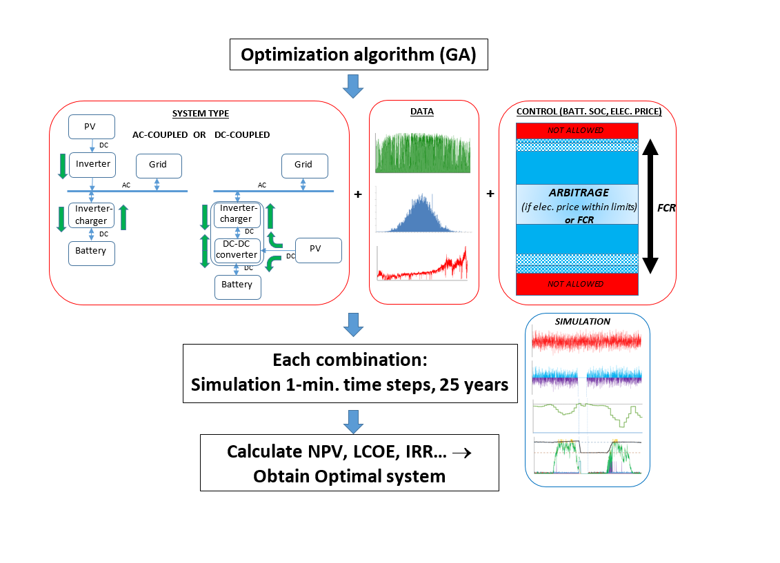
Optimising a PV-plus-battery system is complex. Various combinations of technologies and sizes of PV generators, batteries, inverters/chargers, and set points for control strategies can be considered. For each combination, the system’s performance must be simulated during the system lifetime in steps of 1 min, considering battery degradation, PV derating, and changes in irradiation and electricity prices during the years. After the simulation of each combination is performed, we can calculate the economic results (net present cost, NPC, and others). After all combinations have been evaluated (or a fraction of them, if using GA), obtain the optimal system. Figure 1 shows the PV-plus-battery system in both AC- and DC-coupled versions [5] (the efficiencies shown in Figure 1 are defined later in Section 2.4). The DC-coupled inverter-charger includes a DC-DC converter.
The following subsections present the optimisation objective, applied metaheuristic technique (GA), economic calculations, and detailed system simulation.
2.1. Optimisation Objective
The software simulates, in time steps of one minute during the system lifetime (typically 25 years, equal to the expected PV lifetime), different combinations of possible components (PV generator, inverter/charger, battery) and control strategies (set points for arbitrage and FCR). The objective of the optimisation is to maximise the NPV of the system (the difference between the present value of cash inflows and that of cash outflows over the system’s lifetime [33]), as calculated in Section 2.3. Subject to the following constraints (Equations (1)-(3)).
- The total investment cost cannot exceed a maximum (M€).where is the CAPEX of component j (PV cell, battery, and inverter/charger).
- The total land the system uses must not exceed the maximum allowable (ha).where (MW) and (MWh) are the PV and battery sizes, respectively; (ha/MW) and (ha/MWh) are the specific land uses, respectively.
- The capacity factor (CF) is defined here as the total energy injected (sold) to the grid (, calculated in Section 2.5) during the system lifetime (years) divided by the maximum energy that can be injected into the grid. CF must be higher than the minimum capacity factor .where (MW) is the maximum power that can be injected into the grid (grid power limit).
These constraints are defined by the designer, considering the maximum cost of the inverters, the maximum land available for the project, and the minimum capacity factor, which determines the minimum efficiency of the system (considering the maximum capacity of the grid). In some countries, this regulation is required.
2.2. Genetic Algorithms
The software employs the GA for optimisation if the computation time is extended. Two GAs were used: a main GA to optimise the combination of components and a secondary GA to optimise the control strategy (for each combination of components considered).
The vectors of the variables to be optimised are as follows.
Five variables are optimised for the main GA (optimisation of components). Figure 2 shows the vector of variables that represents each individual (possible solution) in the main GA.
These variables are integer values. is the code for the PV generator type (in AC-coupled, it includes its inverter), is the number of PV generators of the type in parallel, is the code for the battery type, is the number of batteries in parallel, and is the code for the inverter-charger type.
Four variables are optimised for the secondary GA (optimisation of the control strategy, that is, the variables to decide between arbitrage and FCR in each time step). Figure 3 shows the vector of these variables.
These variables are float values obtained between a minimum and maximum in a specific number of steps. The values of are in the range of the sold electricity price (between minimum and maximum), while the values of are between minimum and maximum SOC allowed for the battery (typically between 10 and 100%).
and are the price variables to determine if the system operates under arbitrage or FCR conditions, as the electricity price is compared to these values at the beginning of each service period (every 4 h or 1 h, depending on the service period selected), as shown in Figure 4, where t is the time (min), from 0 to the end of the system lifetime (, usually 25 years): 60 min/h·24h/day·365day/yr·25yr = 1.314·107 minutes. In the flowchart in Figure 4, is the hour of the day, is the minute of the hour, and is the hour of the day when the FCR service period starts; if the service period is 4 h, is 0, 4, 8, … 20, whereas if the service period is 1 h, is 0, 1, 2, … 23.
is the minimum electricity price necessary for the discharge under arbitrage operation: if the price of electricity at a given hour is higher than (and ), the batteries must be discharged, and electricity must be injected into the AC grid. is the maximum price required for the charge under arbitrage operation: if the price at a particular hour is sufficiently low (less than , and ), the batteries will be charged using renewable power. If none of the above conditions are met, the batteries are used for the FCR.
and are the minimum and maximum SOC of the battery for the arbitrage operation, respectively. Under the arbitrage operation, the battery charges up to the limit, and when discharging the battery, it discharges to the limit.
Figure 4 shows a flowchart that clearly illustrates the procedure followed to determine arbitrage or FCR at the beginning of each service period.
The secondary GA obtains the optimal control for each combination of components the main GA considers (Figure 5).
The main GA begins with the first generation: the random generation of Nm vectors (Ngen_main =1). For each vector of the main GA, the secondary GA runs to obtain its optimal control: first generation (Ngen_sec = 1, random generation of Nsec vectors); then, it calculates NPV and fitness; selection, crossing, and mutation are performed to obtain a new generation, which is repeated until the maximum number of generations of the secondary GA is evaluated (Ngen_sec_max) to obtain the best control. Each vector of the main GA (with its optimal control obtained by the secondary GA) is evaluated (its NPV is known, and its fitness is calculated), and then selection, crossing, and mutation are used to obtain a new generation of the main GA. The process is repeated until the maximum number of generations of the main GA has been evaluated (Ngen_main_max), and the optimal combination (components and control) is the minimum NPV.
The fitness function of combination i of the main algorithm is assigned according to its rank in the population (rank 1 for the best individual, the one with the maximum NPV, and rank Nm for the worst solution, that with the minimum NPV). Equation (4) [32,33]:
A similar equation is used to obtain the fitness of the secondary algorithm.
Proportional selection (roulette), one-point crossover, and non-uniform mutation are used to obtain the parents of each new generation. In a previous study, we obtained the optimal parameters of a typical GA to optimise standalone hybrid renewable energy systems [35].
2.3. NPV, LCOE and IRR Calculation
The NPV of each combination of components i and control strategy k evaluated () is computed using Equation (5), which considers the income from selling electricity to the grid and from the FCR service during the system lifetime LifeS (years) and all costs during the same period: the CAPEX and OPEX of all the components of the system, their replacement cost during the system lifetime, and the cost of electricity purchased from the AC grid.
where NPCrep_j is the sum of the present costs owing to replacements of component j (PV, battery and inverter/charger) during the system lifetime (PV lifetime is the same as the system lifetime, battery lifetime depends on its performance; inverter-charger lifetime is a fixed value, usually 10-15 years). CostO&M_j is the annual OPEX of component j at the beginning (year 0); Costpurch_E_y is the cost of the electricity purchased from the AC grid during year y (1…LifeS); Incsell_E_y is the income owing to the electricity sold to the AC grid during year y; IncFCR_y is the income from FCR service during year y; Inf is the annual inflation rate and I is the annual nominal interest or discount rate.
The electrical energy income ( owing to the energy injected into the grid and owing to the FCR service), as well as the costs () during year y, are calculated using Equations (6)-(8).
where Esell(t) and Epurch(t) are the electrical energy sold (injected) to the AC grid and the electrical energy purchased from the AC grid during each time step of year y (MWh), respectively; PrEsell(t) and PrEpurch(t) are the prices of electrical energy sold to the AC grid and of the electrical energy purchased from it during each time step of year y (€/MWh), respectively; is the first minute of the year y; PFCR(per) and PrFCR (per) are the FCR power bid offered (MW) and the FCR price (€/MW) of each FCR service period (duration of 4 h or 1 h), respectively; is the first period of the year and Nper is the number of FCR service periods in one year (8760 h / 4 h = 2190 in the case of 4 h periods or 8760 in the case of 1 h periods).
It is assumed that our PV-plus-battery system is a price-taker. The electricity price differs every hour (real-time pricing (RTP)). The hourly price of the first year can be converted to the rest of the year using the estimated annual inflation. The effect of the change in the hourly profile of the day owing to the increase in PV penetration (“duck curve”) and the increase in wind penetration is accounted for using Equation (9) [36].
where is the sell electricity price per hour h (0… 8760) of year y, and are the PV and wind factors to consider the price reduction in the future hourly price profile owing to the increase of PV and wind penetration, is the annual inflation rate for the electricity price. The purchase price of electricity is affected similarly.
The FCR service price is expected to be affected by inflation in electricity prices (Equation (10)).
where is the FCR service price of period per of year y.
The price variables to determine whether the operation is arbitrage (charge or discharge) or FCR during each time interval, and , are updated every year with the electricity price inflation to ensure that this price is compared to their updated values shown in Figure 4.
The levelised cost of energy () is calculated as the net present cost (NPV total minus present income) divided by the sold energy affected by electricity inflation and the nominal interest rate (Equation (11)).
The internal rate of return () is calculated for each combination of component i and control strategy k, which is the discount rate that makes the = 0.
2.4. Simulation
Each combination of components and control strategy is simulated during the lifetime of the system in steps of 1 min. A simulation of the system is presented in the following subsections (see Figure 1 for reference).
2.4.1. Irradiation and PV Generation
Global and diffuse hourly irradiation data over the tilted surface were downloaded from different databases (PVGIS [37]), Renewables Ninja [38], or NASA [39] for a typical year, which is the irradiation of year 1, . The irradiation for each hour (h) of each year (y) of the system lifetime, (W/m2), is obtained by modifying the downloaded hourly irradiation data using a random number following a normal distribution with mean 0 and standard deviation [36] (Equation (12)):
For each time step (1 min) t (from 0 to the end of the system lifetime, , after obtaining the global and diffuse minute irradiance data (Ghours(t) and Dhours(t)), the irradiance in 1-min time steps G(t) (W/m2) is calculated through a first-order autoregressive (AR) function () [36] (Equations (13)-(14)).
where is the correlation factor and is the standard deviation.
The DC-power PV-generator output is calculated in Equation (15) [36]:
where is the peak power of the PV generator (MWp), is the PV annual reduction factor owing to degradation, is the loss factor, α is the power temperature coefficient of the PV module (%/ºC), and are the irradiance and the cell temperature under standard conditions and (ºC) is the PV cell temperature during time t, which is obtained using Equation (16).
where NOCT is the nominal operation cell temperature (ºC) and is the ambient temperature (ºC), considered a constant during each hour (also downloaded from PVGIS, Renewables Ninja or NASA).
For bifacial PV modules, the irradiance over the back surface, Gback(t) (W/m2), was obtained following the methodology described by Durusoy et al. [40]. By defining the bifaciality (
) as the ratio of the rear power to the front power of the PV module (under STC), the power generated by the bifacial PV generator is calculated using Equation (17).
Equation (17) is similar to Equation (15) by simply adding the contribution of the PV generation of the back surface (adding the factor to the front irradiation).
In AC-coupled systems, the PV power is converted to AC through its inverter, whose efficiency () depends on its output power and is limited to its rated power () (curtailment: clipped energy when the DC output PV power exceeds the rated power of the inverter, which depends on the ILR (DC/AC ratio), which is approximately 1.3 [8]).
Equation (18) shows that the maximum AC output power is the inverter-rated power (
In DC-coupled systems (Equation (19)), if the strategy determines that the PV must inject power into the grid, the PV DC power is converted to AC through the inverter/charger, whose efficiency () also depends on the output power; the AC power is limited by the inverter power ().
where is the DC-DC converter efficiency of the DC-coupled inverter charger.
2.4.2. Battery Charge and Discharge
Depending on the operation (arbitrage or FCR, charge, or discharge, as shown in Figure 4), the battery is charged, discharged, or remains in the float state for each time step.
2.4.2.1. Arbitrage, Battery Charge
If, during a time step, the operation is arbitrage and battery charge, the battery will be charged with the PV power, considering that it cannot be higher than i) the power of the charger of the inverter charger, ii) the maximum power allowed by the battery, and iii) the power to charge the battery in the time step to the maximum SOC allowed for arbitrage. The charging power that enters the battery under an arbitrary operation, , is calculated considering the different efficiencies shown in Figure 1 using Equation (20) (DC-coupled system) or Equation (21) (AC-coupled system).
where (MW) is the rated power of the charger of the inverter-charger (maximum charge current multiplied by the DC battery nominal voltage), (MW) is the maximum charge power allowed for the battery (Li-ion typically 0.5C), SOCmax_arb is the maximum state of charge of the battery allowed for arbitrage operation (energy, MWh), SOC(t) is the energy SOC at the beginning of time step t, is the battery charge efficiency, Δt = 1/60 h and is the charger efficiency of the AC coupled inverter-charger.
2.4.2.2. Arbitrage, Battery Discharge
If the operation is arbitrage during a time step and the battery is discharged, it will be discharged with its maximum power. The discharge power of the battery, , is calculated using Equation (22) (DC-coupled system) or Equation (23) (AC-coupled system).
where SOCmin_arb is the minimum state of charge of the battery allowed for arbitrage operation (MWh), is the battery discharge efficiency and (MW) is the maximum charge power allowed for the battery (Li-ion typically 1C).
Figure 6 shows the battery capacity bands used for the arbitrage and FCR.
2.4.2.3. FCR
Suppose FCR operation is initiated during a service period, which can be either 1 hour or 4 hours. The bidirectional FCR power that the battery can provide for that period is calculated based on specific regulations. In Germany, since 2019, the maximum offered bidirectional FCR power must be sustainably available for at least 15 minutes (= 0.25 h) at any point within the service period. Additionally, the FCR provider is required to maintain a buffer of 25% over its prequalified power (=1.25) [23]. The minimum bid is 1 MW, and the minimal increment is also 1 MW. The maximum offered bidirectional FCR power is determined using Equation (24) for AC-coupled systems.
For DC-coupled systems, the same equation applies; however, it includes the DC-DC efficiency within the battery charge and discharge efficiencies.
Where SOCmin = FSOC_minCn and SOCmax = FSOC_maxCn_y are the minimum and maximum SOC allowed for battery operation (MWh) (Figure 6), respectively, Cn_y is the remaining rated energy capacity of the battery (MWh) (for year 1, it is the rated capacity, Cn; in the following years, owing to degradation, the remaining capacity is reduced annually until its replacement). FSOC_min and FSOC_max are the factors used to calculate the minimum and maximum allowed SOC, respectively. As the capacity of the battery is continuously decreasing because of its degradation (cycling and calendar), SOCmax is being reduced until the battery is replaced (when its remaining capacity drops to a specific percentage of the rated capacity, typically 80%, that is, when the capacity loss reaches 20%); in this study we update SOCmax at the end of each year, considering degradation.
Once the FCR power bid offered is determined for each period, the charge or discharge power is set for every time step, considering that discharge occurs during time steps when the deviation from the nominal frequency is positive (Δf(t) = fn – f(t) >0), and charge occurs during time steps of negative deviation (Δf(t)<0) [41]. The charge/discharge power, and , is linearly proportional to the deviation Δf(t), with a maximum at Δƒ= ±0.2 Hz. When |Δƒ(t) | > 0.2 Hz, the battery is charged or discharged with the full offered FCR power. The insensitivity range of the frequency control (dead band) is Δƒ(t)= ±10 mHz (within these limits, the battery is not charged or discharged). Equations (25)–(26) detail how the charge and discharge power is adjusted based on frequency deviation, as explained above.
The previous equations are valid for AC-coupled systems; for DC-coupled systems, the same equations apply, multiplied by the inverter and charger efficiencies and the DC-DC efficiency.
If during time step t, the PV power is higher than , the battery is charged with the available power from the PV (not exceeding the maximum allowed), provided SOC is lower than the maximum SOC for arbitrage (Equation (27) for DC-coupled system and Equation (28) for AC-coupled system). When SOC is higher than that value, to prevent a high SOC at the end of the time step and a lower probability of obtaining a high FCR power bid for the next period, if the Boolean variable is 1, the charge is limited to the value obtained in Equation (26).
When Δƒ(t) is within the dead-band and the battery SOC(t) is higher/lower than a set point SOCmax_corr_start / SOCmin_corr_start, a corrective discharging/charging power (at a specific C-rate Crate_corr) will be applied until the battery drops from/reaches a set point SOCmax_corr_stop / SOCmin_corr_stop [41] (Figure 6).
2.4.2.4. Battery SOC
The SOC at the beginning of the next time step (minute t+1) is calculated using Equation (29) when charging or discharging, and with Equation (30) during the float stage (when neither charging nor discharging).
where is the monthly self-discharge factor (approximately 1–3%).
2.5. Energy Sold and Purchased to/from the Grid
The energy sold (injected) to the AC grid is calculated according to Equation (31). For any given time step t, the sell energy is determined by the minimum of several factors.
where is the AC auxiliary consumption of the storage system, which includes cooling, heating, instruments, control, lighting, and battery management system -BMS- control.
For an AC-coupled system, the calculation adjusts as shown in Equation (32).
The total energy sold during the system lifetime is calculated using Equation (33).
For energy purchased from the AC grid in a DC-coupled system, refer to Equation (34).
For an AC-coupled system, the energy purchased calculation adjusts as in Equation (35).
Finally, the total energy purchased during the system lifetime is given by Equation (36).
2.6. Li-ion Battery Ageing Model
There are different Li-ion technologies [42]; in this study, we consider the lithium iron phosphate (LFP) type, which is typical for this type of application. Regarding cycle ageing [43] and calendar ageing [44], we use the model proposed by Naumann et al., which was obtained by testing LiFePo4/graphite cells (commercial model Sony US26650FTC1). Capacity fading is caused by cycle ageing (Equation (37), dependent on the complete equivalent cycles performed and considering the effect of the depth of discharge DOD and the charge/discharge rate) and calendar ageing (Equation (38), considering the impact of temperature, SOC and time).
where (%) is the percentage of capacity loss owing to cycling when full equivalent cycles (energy discharged by the battery divided by the battery energy capacity) are cycled at a C-rate and depth of discharge . (%) is the percentage of capacity loss owing to the calendar when a time (min) has passed with an average charge level SOC and average temperature T (K). is the activation energy (17126 Jmol-1), R = 8.314 Jmol-1K-1 is the universal gas constant, is the reference temperature (298.15 K), and , a, b, c, d (for cycling or for calendar) and z are constant parameters shown in references [43] and [44], respectively, which can be modified to fit the ageing performance of another manufacturer’s battery.
The full equivalent cycles of charge-discharge during the system lifetime are accounted for in 11 intervals (is the number of full equivalent cycles performed by the battery at 0.1–2% of DOD, and is the average of the range, that is, 0.01; is the number of FEC at 2–10% of DOD and = 0.06; … is the number of FEC at 90–100% DOD and = 0.95). Equation 39 includes the sum of all the contributions of the DOD ranges.
Equations (37)–(38) are calculated at the end of each year, comparing the total loss (%) with the maximum loss allowed (, generally considered as 20 or 30% of Cn). When the total loss reaches , the battery end of life is reached, and the battery must be replaced (currently, are reset to 0). A maximum operating life of 20 years is considered for stationary battery systems [44].
The battery remaining capacity at the start of each year y is calculated using Equation (39).
3. Results and Discussion
This section presents the results of this study and addresses the research questions listed in Section 2. A base case located in Wiesenthal, Germany, was optimised. After that, a sensitivity analysis was performed to evaluate the effects of certain variables.
The following subsections explain the data, results, and sensitivity analysis.
3.1. Base Case Data
A system was optimised near Wiesenthal, Germany (latitude 50.70 °N, longitude 10.18 °E). The following subsections present the irradiation and temperature data, FCR data, component features and costs, and electricity prices.
3.1.1. Irradiation and Temperature
The hourly irradiation and temperature data were downloaded from the PVGIS [37] database (data for the year 2020). Figure 7 and Figure 8 show the hourly irradiance at an azimuth (south-faced) horizontal axis tracking. The annual irradiation over the front surface was 1,432 kWh/m2, whereas the back irradiation was 306 kWh/m2 (albedo 0.2). Figure 9 shows the hourly temperature data for 2020.
3.1.2. FCR
The average frequency for each minute of the year 2022 has been calculated using frequency data available at [45]. Figure 11 shows the frequency for one week in July.
The price for the FCR used is based on data downloaded from [46], and corresponds to the entire year 2023. Figure 12 shows the prices for the first week of July 2023.
An FCR service period of 4 h was considered in the base case (the German case, with data shown in Section 2.4.2.3). The correction set points were as follows: SOCmax_corr_start = 80%, SOCmin_corr_start =20%, SOCmax_corr_stop = 70%, and SOCmin_corr_stop= 30% with a power rate of Crate_corr = 0.125.
3.1.3. Costs
The cost assumptions were based on the utility-scale data storage (60 MW/240 MWh) from Ref. [47]. The storage CAPEX cost, including all costs (including inverter-charger and extra costs: BOS, taxes, installation labour, permitting fees, overheads, and contingencies), for a 4 h duration storage in the USA, Q1 2022, was approximately 430 €/kWh (Li-ion standalone storage system [47]). A wide range of costs has been reported in the literature, for example, 321 $/kWh [8] or 575 $/kWh [48].
For the battery cabinet (including battery packs, containers, thermal management system, and fire suppression system), we consider 211 $/kWh, which is affected by a factor of 1.5, to include the extra costs (BOS, taxes, etc.), using a total of 295 €/kWh [47] (considering a euro/dollar exchange rate of 0.93).
For the inverter charger, 116 $/kW was reported in [47], which is also affected by the same factor of 1.5 to include extra costs, resulting in approximately 160 €/kW. The total cost of the Li-ion standalone storage system was 295 €/kWh + (160 €/kW/4h) = 335 €/kWh.
The PV CAPEX (including the inverter) in AC-coupled PV systems without storage was reported to be 0.54 €/Wac for the 5th percentile [49]. This percentile is considered because in PV-plus-battery systems, coupling allows sharing several hardware components between the PV and energy storage systems, which can reduce costs. The PV inverter cost can represent 8% of the total cost of the PV system [47], so the absence of a PV inverter in DC-coupled systems reduces the total cost to 0.5 €/Wdc. For bifacial PV, there are four additional cents per Watt [50].
Batteries are expected to reduce their cost annually by 4 % (cost escalation of 4%/year [8]). This value calculates the replacement costs during the system’s lifetime (when batteries reach their end of life and must be replaced).
The O&M (OPEX) annual costs for PV were reported to be 10 €/kWac [51]. Considering that the PV and energy storage systems share several hardware components, we estimate the PV OPEX to be 1% of the PV CAPEX in this work. For the battery, we considered 1% of the battery CAPEX [52] (higher OPEX costs are reported by NREL [53], which include battery replacement costs, which are considered separately in this study).
BESS in Germany are exempt from many network costs and other charges that usually apply to regular consumers. Specifically, batteries do not have to pay network fees and the electricity tax [54].
The financial costs are the nominal discount rate I = 7% and general inflation rate Inf = 2%. The duration of the study was 25 years. The total CAPEX of the system should be obtained through a loan with a 7% interest rate for 25 years.
According to the European Central Bank projections, inflation in Germany is expected to gradually decrease in the coming years, reaching 2.4% in 2024 and 2.0% in 2025 [55]. The Deutsche Bundesbank also provides detailed inflation forecasts. According to their projections, inflation in Germany follows a downward trend [56]. These forecasts suggest that, for economic studies over 25 years, a reasonable average annual inflation rate for Germany could be around 2%.
3.1.4. Electricity Price
At the beginning of the system (year 0), the hourly electricity spot price for 2023 in Germany [57] (average 0.0952 €/kWh) was considered for the selling and purchasing prices of electricity (Figure 13).
Using Equation (9) with = 0.5, and = 0.2, we obtained the electricity prices, considering = 2% annual inflation for the electricity price.
Figure 14 shows the daily average hourly electricity selling price for the different years; all referred to the 1st year.
3.1.5. Components
Before selecting the component sizes, the maximum grid power must be determined. In this case, = 100 MW. Two types of PV generators were considered, , both, 20 MWdc, one of which was monofacial and the other was bifacial. The number in parallel will be between 4 and 8, (between 80 MW and 160 MW total PV power). For the battery, only one type has been considered, 40 MWh/10MW (4 h duration [8]) (), from 4 to 8 in parallel, (between 160/40 and 320/80 MWh/MW total). For the inverter charger, four types were considered , in steps of 20 MW (40–100 MW). The binary variable was set to 1.
Auxiliary load consumption for the battery (cooling, heating, instruments, control, lighting, BMS control) is considered to be 0.4% of the battery-rated power [58]: = 0.4/100· The ambient temperature of the batteries is supposed to be constant at 20ºC.
The land uses considered in this work were 2.5 ha/MW for PV [59] and 10 ha/GWh for battery storage.
3.2. Constraints
The constraints were as follows: = 250 M€, = 400 ha, maximum 160 MW (PV-only), and = 0.2. The maximum land use implies a PV-only system with a maximum of 160 MW. A minimum capacity factor (defined as annual output AC energy divided by the yearly maximum energy that could be injected into the grid considering the grid limit of 100 MW, which is 876,000 MWh) of 0.2 implies a minimum PV monofacial generator of approximately 0.2 · 876,000 / 1432 / 0.8 = 152.9 MW (considering 1432 kWh/m² annual irradiance on the front surface and a performance ratio of 0.8). These constraints are valid since we have two types of PV generators (monofacial and bifacial), and the system includes BESS.
3.3. Base Case Optimisation Results
The simulation used an Intel i5-6500 CPU (3.2 GHz and 16 GB RAM). In addition, the simulation (during 25 years in 1-minute time steps) and evaluation of each combination of components and control was for 17.8 s. The parameters for the selected GA were as follows: maximum number of generations, 10; population, 7 for the main GA and 15 for the secondary GA; crossover rate, 70%; and mutation rate, 1%. For each optimisation, evaluating all combinations would have taken 66 days, whereas using the GA took one day and 9 h. Table 2 lists the optimal systems determined by the GA for the AC-coupled- and DC-coupled systems. The energy values are averaged yearly (different for each year).
The optimal control of PV-plus-battery systems employs FCR and arbitrage. Similar to the works of Biggins et al. [29] and Naemi et al. [31], we found that the combination of arbitrage and FCR improves economic results. Using tight-band arbitrage can provide significant income and not impede the storage’s ability to provide FCR services. In another study, Pusceddu et al. [30] showed the potential synergies between the provision of FCR and arbitrage in the same way.
The results show that AC-coupled systems are more profitable (higher NPV and IRR, and lower LCOE) than DC-coupled systems. In addition, the capacity factor was slightly higher for AC-coupled systems. The highest incomes are because of selling PV generation directly, whereas FRC incomes account for approximately 15% of the total income. The PV generator included in the optimal configuration is bifacial. The ILR for AC-coupled was 1.25, and for DC-coupled it was 1.4. Moreover, BIR was 1 for the AC-coupled and 0.4 for the DC-coupled. The battery lifetime obtained in the degradation model was 19.8 years for AC-coupled and 20.4 years for DC systems, which are higher than the maximum operating life for stationary battery systems (20 years); this is the final value considered in the economic calculations.
The system without storage (PV-only system of 160 MWdc) has an NPV 56% higher than that of the optimal AC-coupled PV-plus-battery system, indicating that storage, with the present costs and considering the electricity fees used in this study, is not profitable.
Figure 16 shows the simulation of the optimal AC-coupled system over two consecutive days (year 12, January 1st–2nd). The FCR operation is selected for all the time except for 4 hours (from 12:00 to 16:00 on the second day) when there is arbitrage and discharge. At 12:00, the SOC is higher than the minimum SOC for arbitrage, and the electricity price is higher than the set point limit. Therefore, arbitrage and discharge are selected for the next 4 hours. In PV generation, there is a limitation in PV production because of its inverter (ILR=1.25; rated power of the inverter is 112 MW) and the injected energy limit of the power grid (100 MW).
Figure 17 shows the simulation of the optimal DC-coupled system for the same two consecutive days, where the FCR service is used throughout the day (no arbitrage). In Figure 17, we can see the curtailment (to the limit of 100 MW) in the power injected into the grid due to the inverter-charger power limit.
In both figures, the maximum and minimum SOC for arbitrage are the percentages shown in Table 2 multiplied by the battery’s maximum capacity during year 12.
For comparison purposes, we again optimised the PV-plus-battery AC-coupled system using a discrete version of the particle swarm optimisation (PSO) algorithm [61] with the following parameters: number of epochs = 20, population = 500, cognitive coefficient = 2, and social coefficient = 2. PSO was programmed to optimise the components and control strategy using a unique algorithm (all variables were codified in a unique vector). The optimal PV-plus-battery AC-coupled system obtained by PSO has an NPV of 76.54 M€, slightly lower than the optimal obtained using GA (77.35 M€). The components are the same, but the control strategy is different. With PSO, the arbitrage price limits are 0.176 and 0.352 €/kWh, and the arbitrage SOC limits are 30% and 50%. In this study, GA obtained better results than PSO, possibly because GA uses two algorithms, while the PSO algorithm has been programmed with a single algorithm to reduce complexity. Figure 18 shows the evolution of both algorithms.
3.4. Sensitivity Analysis
The sensitivity analysis of the most relevant variables was evaluated by repeating the optimisation for each case.
3.4.1. Cases of
= 0, no FCR and 1 h FCR Service
If = 0, that is, there is no extra limitation for when the SOC is higher than the maximum for arbitrage; the NPV variation over the base case as a percentage is shown in Table 3 (NPV is reduced by approximately 20%). In the same table, we can see that the NPV decreases significantly if there is no FCR service, resulting in a reduction of roughly 25% for AC-coupled systems and 45% for DC-coupled systems. This indicates that FCR can be a good source of income for battery systems. In addition, considering a 1 h FCR service instead of a 4 h results in a significantly low increase in NPV.
The FCR service has little impact on the life of the batteries due to the low charge/discharge current, as shown in Table 4.
3.4.2. Cases of Different Inflation of Electricity Prices
The effect of annual electricity price inflation on the NPV of the optimal system is presented in Table 5. Electricity price inflation has a significant impact on NPV (higher in DC-coupled systems).
3.4.3. Cases of Reduction in Battery CAPEX
Table 6 shows the effect of the decrease in battery CAPEX.
For a battery price reduction of 75% (considering only battery cost reduction and no reduction in the inverter-charger), the optimal AC-coupled system has an NPV similar to the PV-only system without storage.
3.5. System Located in Spain
The same system was optimized near Zaragoza, Spain (latitude 41.66 °N, longitude 0.86 °W), considering the same FCR data, component features, and costs, and using the hourly electricity spot price for 2023 in Spain (average 0.0877 €/kWh). Table 7 shows the optimal results, which include the same components as in the Germany optimizations but different control variables and economic results (higher NPV due to higher irradiation in Spain).
In the case of Spain, to achieve an NPV for the AC-coupled system similar to the NPV of the PV-only system, the battery price needed to be reduced by 80%.
4. Conclusions
This paper presents a new method for simulating and optimising utility-scale PV-plus-battery systems considering energy arbitrage and FCR. Unlike previous studies, both AC-coupled and DC-coupled systems were considered, and more accurate models were used in the simulations, using time steps of 1-minute and simulating the entire system lifetime, considering changes in all the relevant variables during the years (irradiation, electricity price, battery degradation, and PV derating). More accurate simulation models imply more accurate economic results and more precise optimisation. The optimisation attempts to determine the most profitable system (with the highest NPV). The optimisation variables are the sizes of the components and the control set points (the limit electricity prices for charge/discharge and the SOC limits for the arbitrage operation). Each combination of components and control strategy was simulated in 1-minute steps during the system lifetime (typically 25 years). Owing to the inadmissible computation times when evaluating all possible combinations, optimisations were performed using the GA. Unlike previous studies, this study considers advanced battery degradation models (for cycling and calendar) and PV derating, different irradiation, and hourly electricity price curves for each year of the system lifetime. In addition, the auxiliary load consumption of the storage system and variable inverter efficiencies were considered.
A particular case study of Wiesenthal (Germany) has been shown, with present components cost, hourly electricity price in 2023 in Germany (estimating the prices of the rest of the years with the effect of the increase or renewable penetration, “duck curve”) and FCR service prices in Germany (4 h service periods), considering a yearly inflation rate of electricity and FCR service of 2%. The optimal system includes a small SOC range for arbitrage (20% to 40% for AC-coupled services and 20% to 60% for DC-coupled services), showing the synergy between arbitrage and FCR services. AC-coupled systems are more profitable than DC-coupled systems (24% higher NPV); however, they cannot compete economically with PV systems without storage, whose NPV is 56% higher than that of AC-coupled PV-plus-battery systems.
The variations in the base cases were evaluated. It can be seen that the limitation for the charge under the FCR service (when SOC is higher than the maximum for arbitrage to avoid excessive SOC and reduction in future FCR incomes) is essential. Otherwise, a significant reduction in NPV is achieved. In addition, systems with only arbitrage (without FCR) achieved significant reductions in the NPV, indicating that FCR services are an essential source of income. By reducing the FCR service period to 1 h, a slight increase in the NPV was achieved. As expected, a reduction in the annual inflation of electricity and FCR service prices (even considering negative inflation values) implies a significant reduction in the NPV. Finally, the effect of the decrease in the battery CAPEX was evaluated. With a 75% reduction in battery CAPEX (from the present value of 295 €/kWh to 74 €/kWh), the NPV of the optimal PV-plus-battery AC-coupled system would be similar to that of the PV system without storage. As in previous studies, we found that combining arbitrage and FCR improves economic results compared to a system with only FCR or arbitrage. The same system was optimized in Zaragoza, Spain (using the hourly electricity price of Spain, 2023), obtaining better economic results due to higher irradiation. Similar conclusions were found for Spain, needing an 80% reduction in battery CAPEX to make AC-coupled PV-plus-battery systems as profitable as PV-only systems.
Author Contributions
Conceptualization, R.D.L. and J.M.L.J.; methodology, R.D.L.; software, R.D.L. and J.M.L.J.; validation, J.L.B.A., J.M.L.J. and J.S.A.S.; formal analysis, R.D.L., J.L.B.A., J.M.L.J. and J.S.A.S; investigation, R.D.L. and J.M.L.J.; resources, R.D.L. and J.L.B.A.; data curation, J.S.A.S.; writing—original draft preparation, R.D.L.; writing—review and editing, R.D.L., J.L.B.A., J.M.L.J. and J.S.A.S; visualization, R.D.L.; supervision, R.D.L.; project administration, R.D.L.; funding acquisition, R.D.L.. All authors have read and agreed to the published version of the manuscript.
Funding
This work was supported by the Spanish Government (Ministerio de Ciencia e Innovación, Agencia Estatal de Investigación) and by the European Regional Development Fund [Grant PID2021-123172OB-I00 funded by MCIN/AEI/ 10.13039/501100011033 and by “ERDF A way of making Europe”].
Data Availability Statement
Data will be made available on request.
Acknowledgments
We wish to thank Dr. Dongwei Zhao for his support in the generation of electricity price curves.
Conflicts of Interest
The authors declare that there is no conflict of interest regarding the publication of this paper.
References
- M. Legrand, R. M. Legrand, R. Labajo-Hurtado, L.M. Rodríguez-Antón, Y. Doce, Price arbitrage optimization of a photovoltaic power plant with liquid air energy storage. Implementation to the Spanish case, Energy. 239 (2022). [CrossRef]
- K. Bassett, R. K. Bassett, R. Carriveau, D.S.K. Ting, Energy arbitrage and market opportunities for energy storage facilities in Ontario, J. Energy Storage. 20 (2018) 478–484. [CrossRef]
- X. Liu, Research on Grid-Connected Optimal Operation Mode between Renewable Energy Cluster and Shared Energy Storage on Power Supply Side, Int. J. Energy Res. 2024 (2024) 21. [CrossRef]
- C. Zhao, P.B. C. Zhao, P.B. Andersen, C. Træholt, S. Hashemi, Grid-connected battery energy storage system: a review on application and integration, Renew, Sustain. Energy Rev. 182 (2023) 1–19. [CrossRef]
- L. Koltermann, K.K. L. Koltermann, K.K. Drenker, M.E. Celi Cortés, K. Jacqué, J. Figgener, S. Zurmühlen, D.U. Sauer, Potential analysis of current battery storage systems for providing fast grid services like synthetic inertia – Case study on a 6 MW system, J. Energy Storage. 57 (2023) 1–8. [CrossRef]
- D. Zhao, M. D. Zhao, M. Jafari, A. Botterud, A. Sakti, Strategic energy storage investments: A case study of the CAISO electricity market, Appl. Energy. 325 (2022) 119909. [CrossRef]
- S. Wilkinson, M.J. S. Wilkinson, M.J. Maticka, Y. Liu, M. John, The duck curve in a drying pond: The impact of rooftop PV on the Western Australian electricity market transition, Util. Policy. 71 (2021) 101232. [CrossRef]
- N. DiOrio, P. N. DiOrio, P. Denholm, W.B. Hobbs, A model for evaluating the configuration and dispatch of PV plus battery power plants, Appl. Energy. 262 (2020) 114465. [CrossRef]
- X. 7 (2021) 8198–8206. [CrossRef]
- R. Dufo-López, Optimisation of size and control of grid-connected storage under real time electricity pricing conditions, Appl. Energy. 140 (2015) 395–408. [CrossRef]
- Y. Energy. 322 ( 2022. [CrossRef]
- Á. Arcos-Vargas, D. Á. Arcos-Vargas, D. Canca, F. Núñez, Impact of battery technological progress on electricity arbitrage: An application to the Iberian market, Appl. Energy. 260 (2020) 114273. [CrossRef]
- T. Terlouw, T. T. Terlouw, T. AlSkaif, C. Bauer, W. van Sark, Multi-objective optimization of energy arbitrage in community energy storage systems using different battery technologies, Appl. Energy. 239 (2019) 356–372. [CrossRef]
- P.E. Campana, L. P.E. Campana, L. Cioccolanti, B. François, J. Jurasz, Y. Zhang, M. Varini, B. Stridh, J. Yan, Li-ion batteries for peak shaving, price arbitrage, and photovoltaic self-consumption in commercial buildings: A Monte Carlo Analysis, Energy Convers, Manag. 234 (2021). [CrossRef]
- F. Wankmüller, P.R. F. Wankmüller, P.R. Thimmapuram, K.G. Gallagher, A. Botterud, Impact of battery degradation on energy arbitrage revenue of grid-level energy storage, J. Energy Storage. 10 (2017) 56–66. [CrossRef]
- Y. Wu, Z. Y. Wu, Z. Liu, J. Liu, H. Xiao, R. Liu, L. Zhang, Optimal battery capacity of grid-connected PV-battery systems considering battery degradation, Renew. Energy. 181 (2022) 10–23. [CrossRef]
- U.G.K. Mulleriyawage, W.X. U.G.K. Mulleriyawage, W.X. Shen, Optimally sizing of battery energy storage capacity by operational optimization of residential PV-Battery systems: An Australian household case study, Renew. Energy. 160 (2020) 852–864. [CrossRef]
- L. Energy Storage. 55 (2022) 105508. [CrossRef]
- Y. Wu, Z. Y. Wu, Z. Liu, B. Li, J. Liu, L. Zhang, Energy management strategy and optimal battery capacity for flexible PV-battery system under time-of-use tariff, Energy. 200 (2022) 558–570. [CrossRef]
- A.H. Schleifer, C.A. A.H. Schleifer, C.A. Murphy, W.J. Cole, P. Denholm, Exploring the design space of PV-plus-battery system configurations under evolving grid conditions, Appl. Energy. 308 (2022) 118339. [CrossRef]
- C. Energy Storage. 50 ( 2022. [CrossRef]
- T. Thien, D. T. Thien, D. Schweer, D. vom Stein, A. Moser, D.U. Sauer, Real-world operating strategy and sensitivity analysis of frequency containment reserve provision with battery energy storage systems in the german market, J. Energy Storage. 13 (2017) 143–163. [CrossRef]
- J. Figgener, B. J. Figgener, B. Tepe, F. Rücker, I. Schoeneberger, C. Hecht, A. Jossen, D.U. Sauer, The influence of frequency containment reserve flexibilization on the economics of electric vehicle fleet operation, J. Energy Storage. 53 (2022). [CrossRef]
- P. Pant, T. P. Pant, T. Hamacher, V.S. Perić, Ancillary Services in Germany: Present, Future and the Role of Battery Storage Systems, (2024). [CrossRef]
- H. Khajeh, C. H. Khajeh, C. Parthasarathy, E. Doroudchi, H. Laaksonen, Optimized siting and sizing of distribution-network-connected battery energy storage system providing flexibility services for system operators, Energy. 285 (2023) 129490. [CrossRef]
- Krupp, R. Beckmann, P. Draheim, E. Meschede, E. Ferg, F. Schuldt, C. Agert, Operating strategy optimization considering battery aging for a sector coupling system providing frequency containment reserve, J. Energy Storage. 68 (2023) 107787. [CrossRef]
- H. Wigger, P. H. Wigger, P. Draheim, R. Besner, U. Brand-Daniels, T. Vogt, Environmental and economic analysis of sector-coupling battery energy storage systems used for frequency containment reserve, J. Energy Storage. 68 (2023) 107743. [CrossRef]
- E. Meschede, U. E. Meschede, U. Schlachter, T. Diekmann, B. Hanke, K. von Maydell, Assessment of sector-coupling technologies in combination with battery energy storage systems for frequency containment reserve, J. Energy Storage. 49 (2022) 104170. [CrossRef]
- F. Energy Storage. 50 (2022) 104234. [CrossRef]
- E. Pusceddu, B. E. Pusceddu, B. Zakeri, G. Castagneto Gissey, Synergies between energy arbitrage and fast frequency response for battery energy storage systems, Appl. Energy. 283 (2021) 116274. [CrossRef]
- M. Clean. Prod. 373 (2022) 133909. [CrossRef]
- M. Gomez-Gonzalez, J.C. M. Gomez-Gonzalez, J.C. Hernandez, D. Vera, F. Jurado, Optimal sizing and power schedule in PV household-prosumers for improving PV self-consumption and providing frequency containment reserve, Energy. 191 (2020) 116554. [CrossRef]
- R. Dufo-López, Software iHOGA / MHOGA, Https//Ihoga.Unizar.Es/En (Accessed , 2023). (2023). 5 May.
- J. Lujano-Rojas, R. J. Lujano-Rojas, R. Dufo-Lopez, J.A. Dominguez-Navarro, Genetic Optimization Techniques for Sizing and Management of Modern Power Systems, Elsevier Inc., Amsterdam, 2023.
- R. Dufo-López, J.L. R. Dufo-López, J.L. Bernal-Agustín, Design and control strategies of PV-diesel systems using genetic algorithms, Sol. Energy. 79 (2005) 33–46. [CrossRef]
- R. Dufo-López, J.M. R. Dufo-López, J.M. Lujano-Rojas, J.L. Bernal-Agustín, Optimisation of size and control strategy in utility-scale green hydrogen production systems, Int. J. Hydrogen Energy. (2023). [CrossRef]
- European Commission, interactive maps, Http://Re.Jrc.Ec.Europa.Eu/Pvgis/ (Visited on 05/13/2023). (2023).
- Staffell, S. Pfenninger, Renewables. ninja, URl Https//Www. Renewables. Ninja/(Visited 03/20/2023). (2020).
- National Aeronautics and Space Administration, NASA POWER Prediction Of Worldwide Energy Resources, Https://Power.Larc.Nasa.Gov/ (Visited on 05/13/2023). (2023).
- B. Durusoy, T. B. Durusoy, T. Ozden, B.G. Akinoglu, Solar irradiation on the rear surface of bifacial solar modules: a modeling approach, Sci. Reports - Nat. 10 (2020) 1–10. [CrossRef]
- R. Hollinger, L.M. R. Hollinger, L.M. Diazgranados, F. Braam, T. Erge, G. Bopp, B. Engel, Distributed solar battery systems providing primary control reserve, IET Renew. Power Gener. 10 (2016) 63–70. [CrossRef]
- M. Armand, P. M. Armand, P. Axmann, D. Bresser, M. Copley, K. Edström, C. Ekberg, D. Guyomard, B. Lestriez, P. Novák, M. Petranikova, W. Porcher, S. Trabesinger, M. Wohlfahrt-Mehrens, H. Zhang, Lithium-ion batteries – Current state of the art and anticipated developments, J. Power Sources. 479 (2020). [CrossRef]
- M. Naumann, F. M. Naumann, F. Spingler, A. Jossen, Analysis and modeling of cycle aging of a commercial LiFePO4/graphite cell, J. Power Sources. 451 (2020) 227666. [CrossRef]
- M. Naumann, M. M. Naumann, M. Schimpe, P. Keil, H.C. Hesse, A. Jossen, Analysis and modeling of calendar aging of a commercial LiFePO4/graphite cell, J. Energy Storage. 17 (2018) 153–169. [CrossRef]
- H. Thiesen, G. H. Thiesen, G. Arne, C. Jauch, Grid Frequency Data – Wind Energy Technology Instiute (WETI) – Flensburg University of Applied Sciences, (2022). [CrossRef]
- Regelleistung.net, Datencenter, (2024).
- V. Ramasamy, J. V. Ramasamy, J. Zuboy, M. Woodhouse, E. O’Shaughnessy, D. Feldman, J. Desai, A. Walker, R. Margolis, P. Basore, U.S. Solar Photovoltaic System and Energy Storage Cost Benchmarks, With Minimum Sustainable Price Analysis: Q1 2023, 2024. [CrossRef]
- U.S. Department of Energy, Battery Storage in the United States: An Update on Market Trends, Batter. Storage United States An Updat. Mark. Trends. (2021) 37.
- Fraunhofer Institute for Solar Energy Systems, Photovoltaics Report, (2014). https://www.ise.fraunhofer.de/en/publications/studies/photovoltaics-report.html.
- EcoWatch, Bifacial solar panels, Tps://Www.Ecowatch.Com/Solar/Bifacial-Solar-Panels (Visited on 05/13/2023). (2023).
- M. Bolinger, J. M. Bolinger, J. Seel, C. Warner, D. Robson, Utility-Scale Solar, 2022 Edition Utility-Scale Solar, 2022 Edition, (2022).
- Asian Development Bank, Handbook on battery energy storage, 2018.
- NREL, Utility-Scale Battery Storage, (n.d.). https://atb.nrel.gov/electricity/2022/utility-scale_battery_storage.
- Engels, B. Claessens, G. Deconinck, Techno-economic analysis and optimal control of battery storage for frequency control services, applied to the German market, Appl. Energy. 242 (2019) 1036–1049. [CrossRef]
- European Central Bank, Economic Bulletin Issue 2, 2024, (2024).
- Deutsche Bundesbank, Monthly Report 24, (2024). 20 March.
- Ember, European wholesale electricity price data, (2024).
- A.J. Crawford, D. A.J. Crawford, D. Wu, V. V Viswanathan, P.J. Balducci,..., Washington Clean Energy Fund: Energy Storage System Consolidated Performance Test Results, (2020). https://www.osti.gov/servlets/purl/1602252.
- NREL, Land Use by System Technology, (n.d.). https://www.nrel.gov/analysis/tech-size.html.
- NREL, Lifetime of PV Panels, (n.d.). https://www.nrel.gov/state-local-tribal/blog/posts/stat-faqs-part2-lifetime-of-pv-panels.html (accessed , 2023). 15 March.
- G. Papazoglou, P. G. Papazoglou, P. Biskas, Review and Comparison of Genetic Algorithm and Particle Swarm Optimization in the Optimal Power Flow Problem, Energies. 16 (2023). [CrossRef]
Figure 1.
AC- and DC-coupled PV-plus-battery system (efficiencies defined in Section 2.4).
Figure 1.
AC- and DC-coupled PV-plus-battery system (efficiencies defined in Section 2.4).
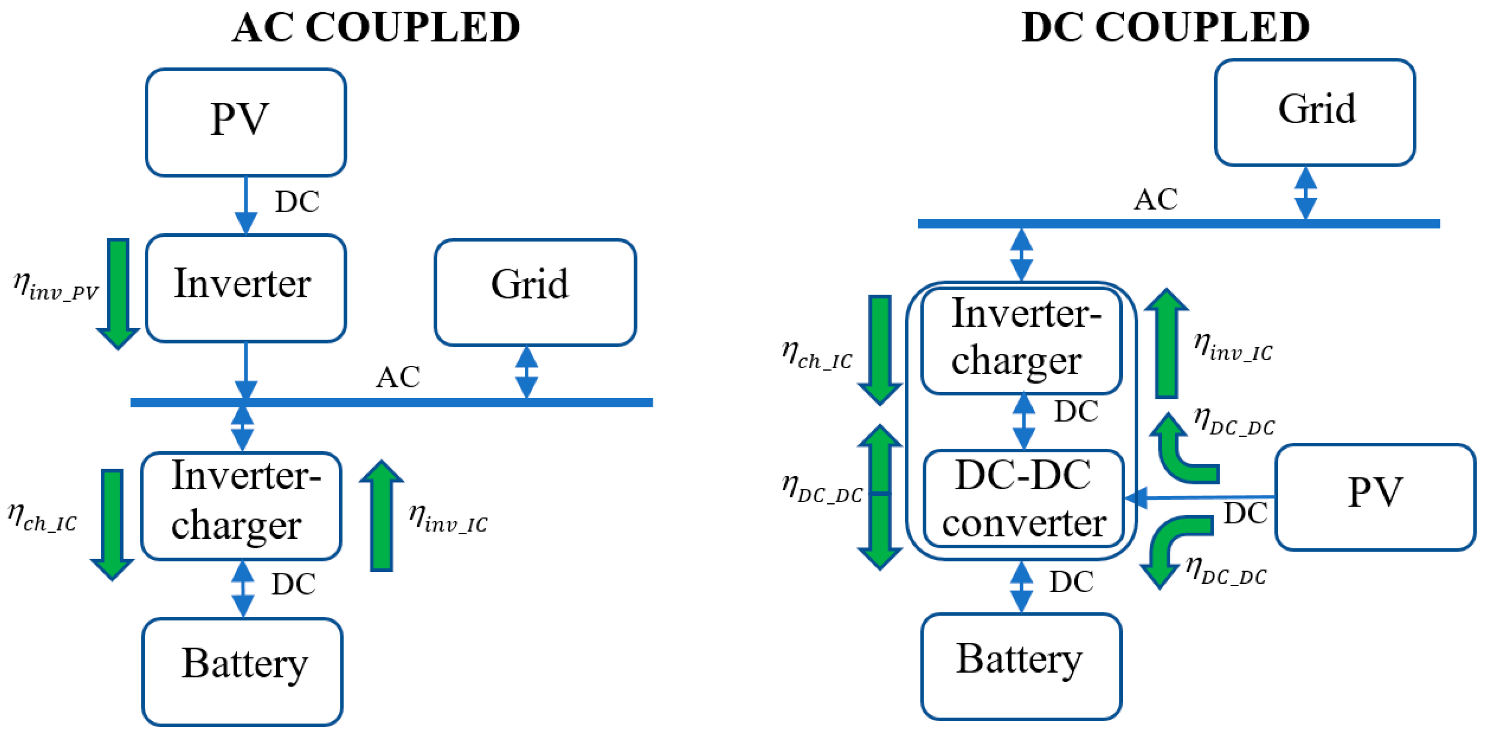
Figure 2.
Vector of variables representing individuals in Main GA.
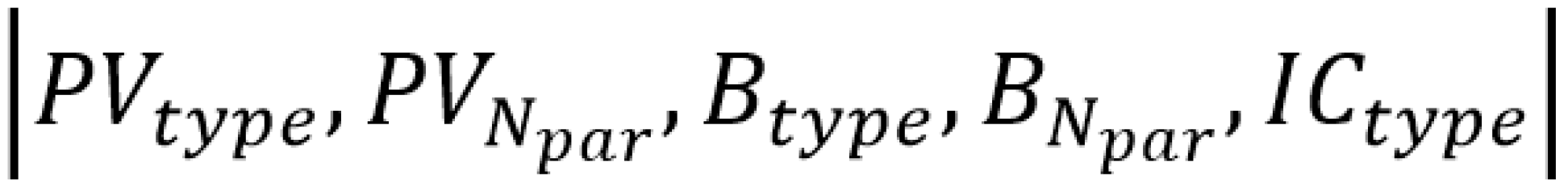
Figure 3.
Vector of variables for control strategy in secondary GA.

Figure 4.
Flowchart to determine arbitrage or FCR at the beginning of each service period.
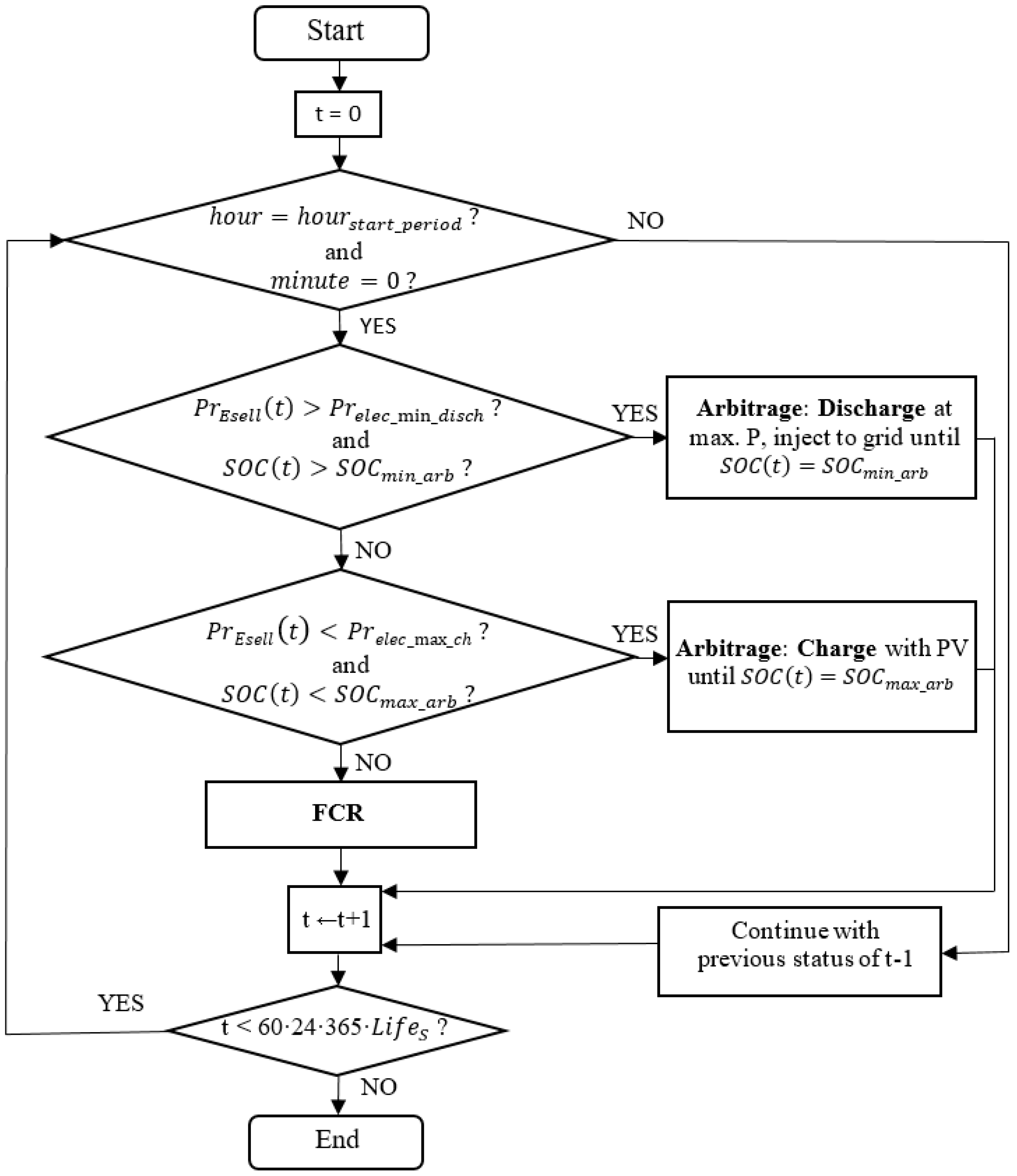
Figure 5.
GA flowchart.
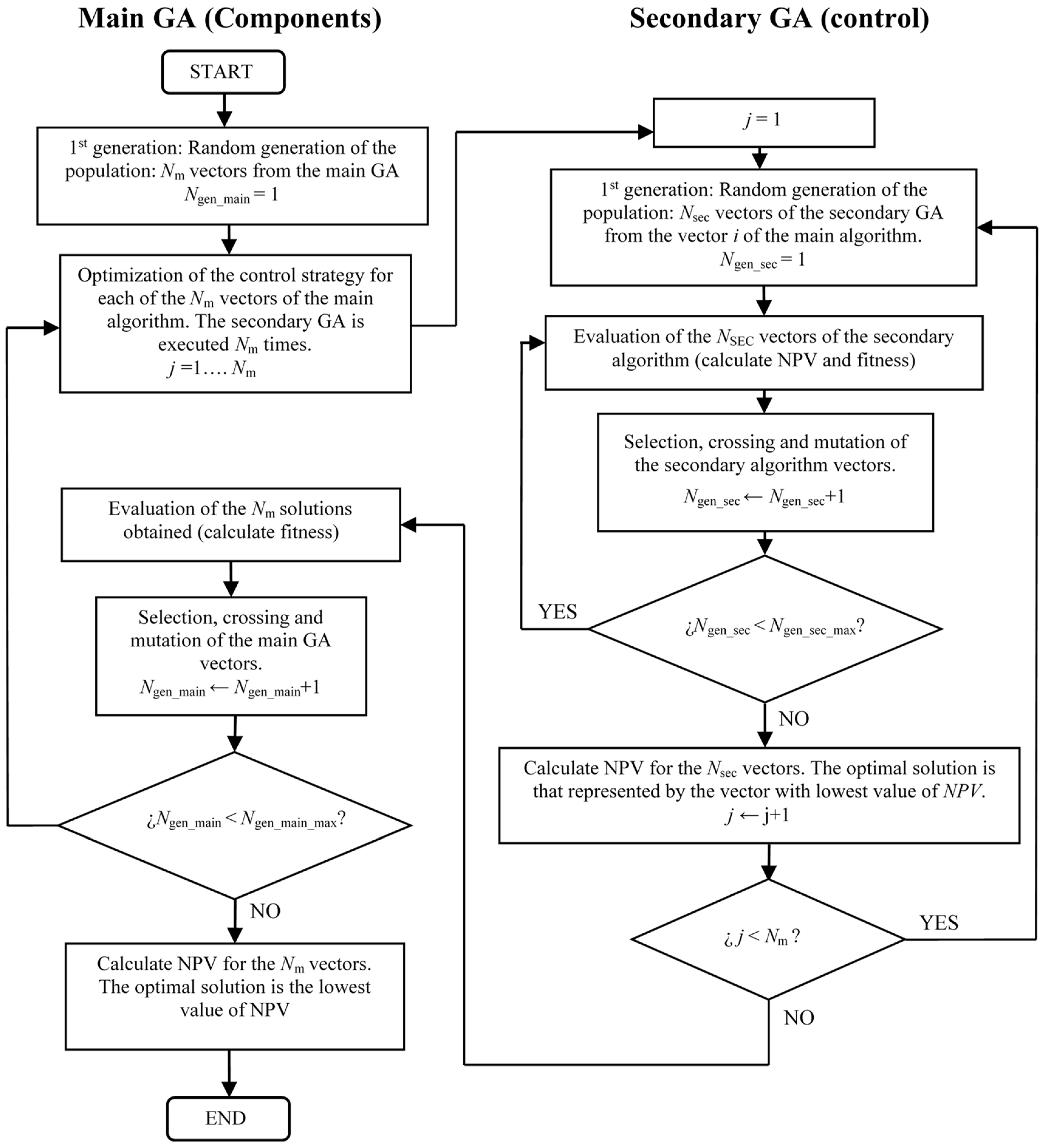
Figure 6.
Battery capacity bands for arbitrage and FCR.
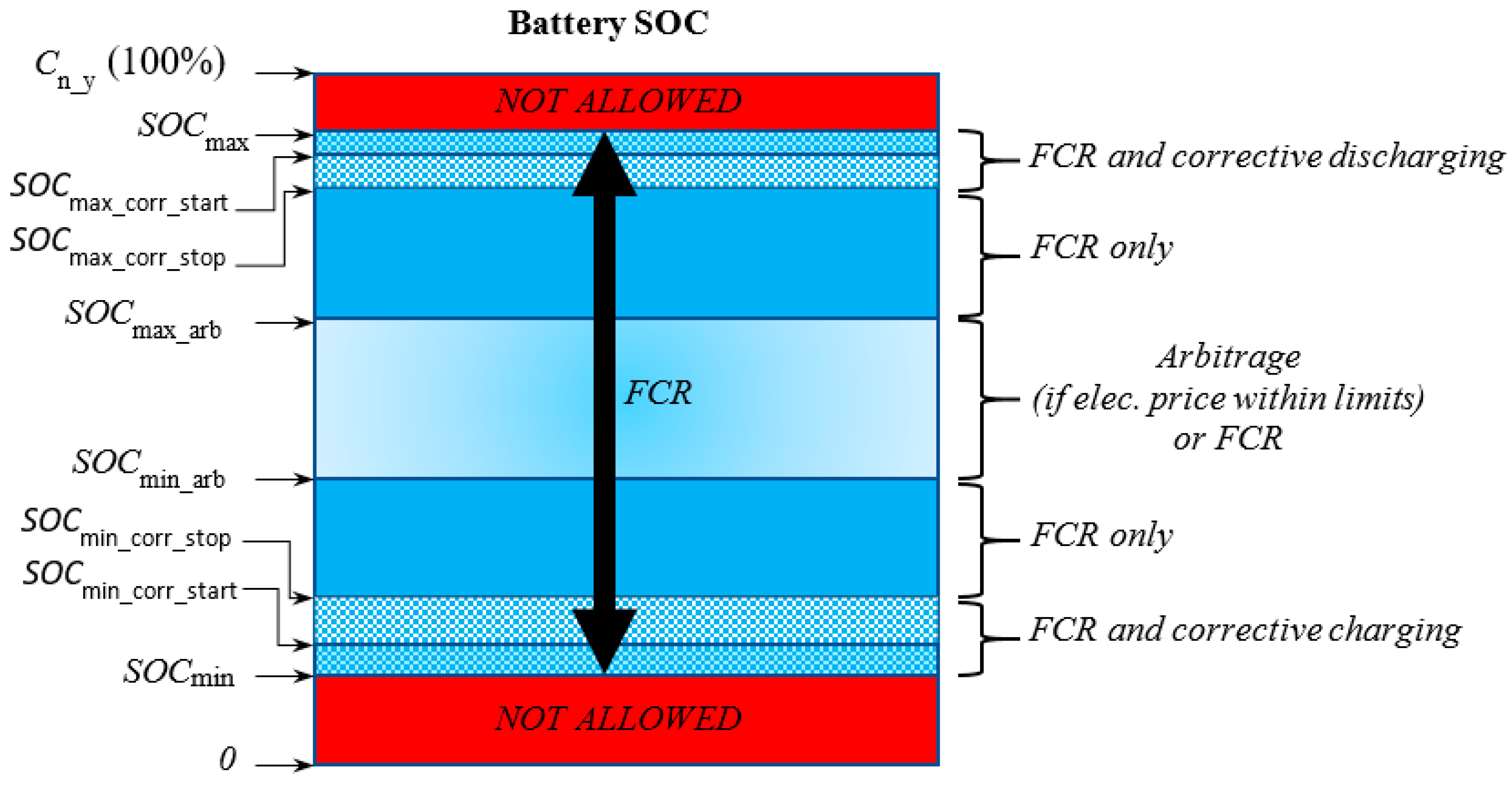
Figure 7.
Hourly Irradiance (front) (kW/m2) near Wiesenthal for 2020 and horizontal axis tracking.
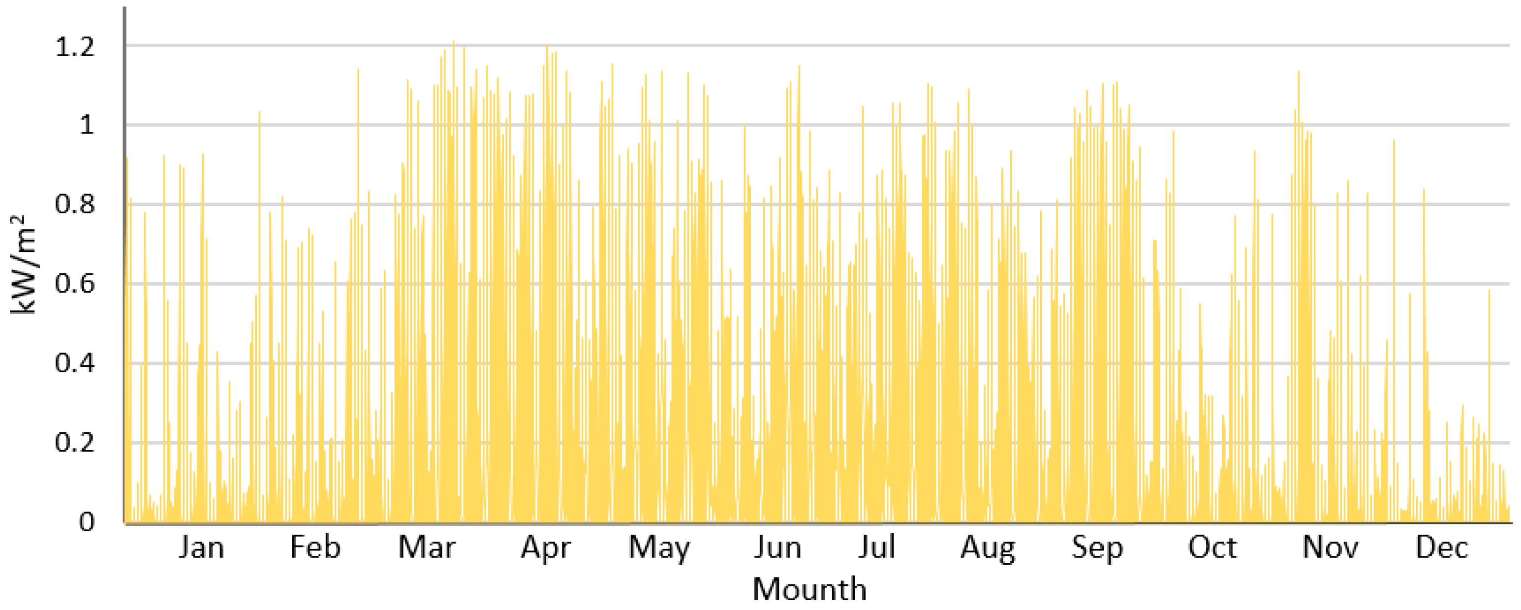
Figure 8.
Hourly irradiance (front) (kW/m2) near Wiesenthal; detail is for 9 days (March-April 2020) and horzontal axis tracking.
Figure 8.
Hourly irradiance (front) (kW/m2) near Wiesenthal; detail is for 9 days (March-April 2020) and horzontal axis tracking.
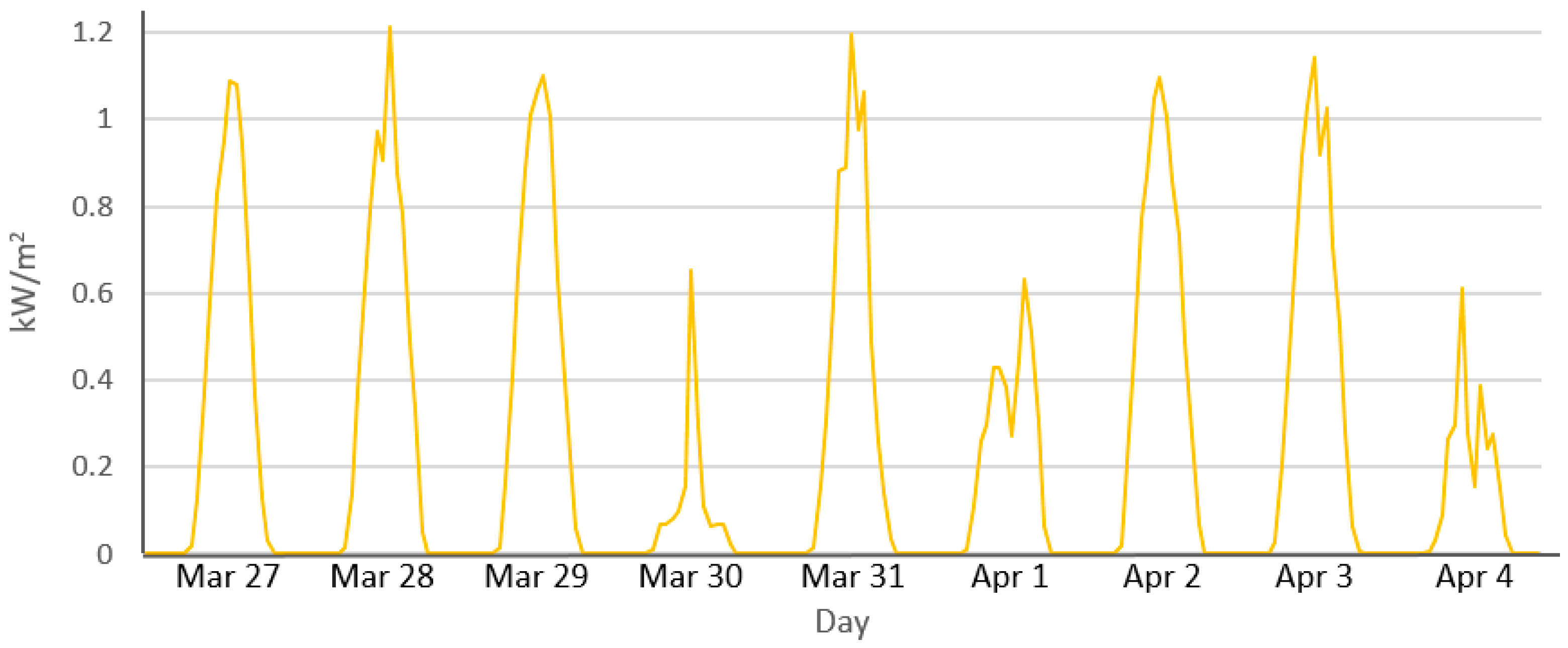
Figure 9.
Ambient temperature (ºC) near Wiesenthal for 2020.
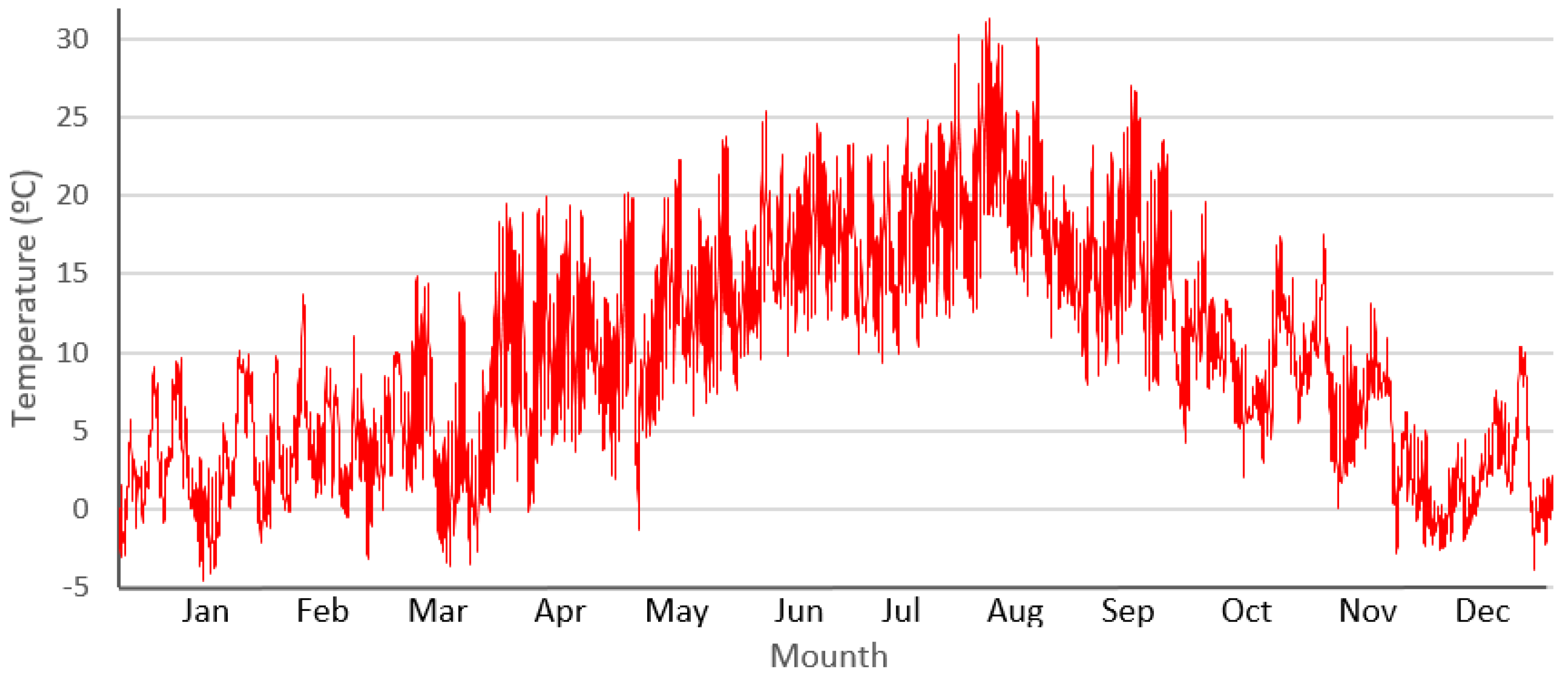
Figure 10.
Annual irradiation over average (%) for the 25 years of the simulation.
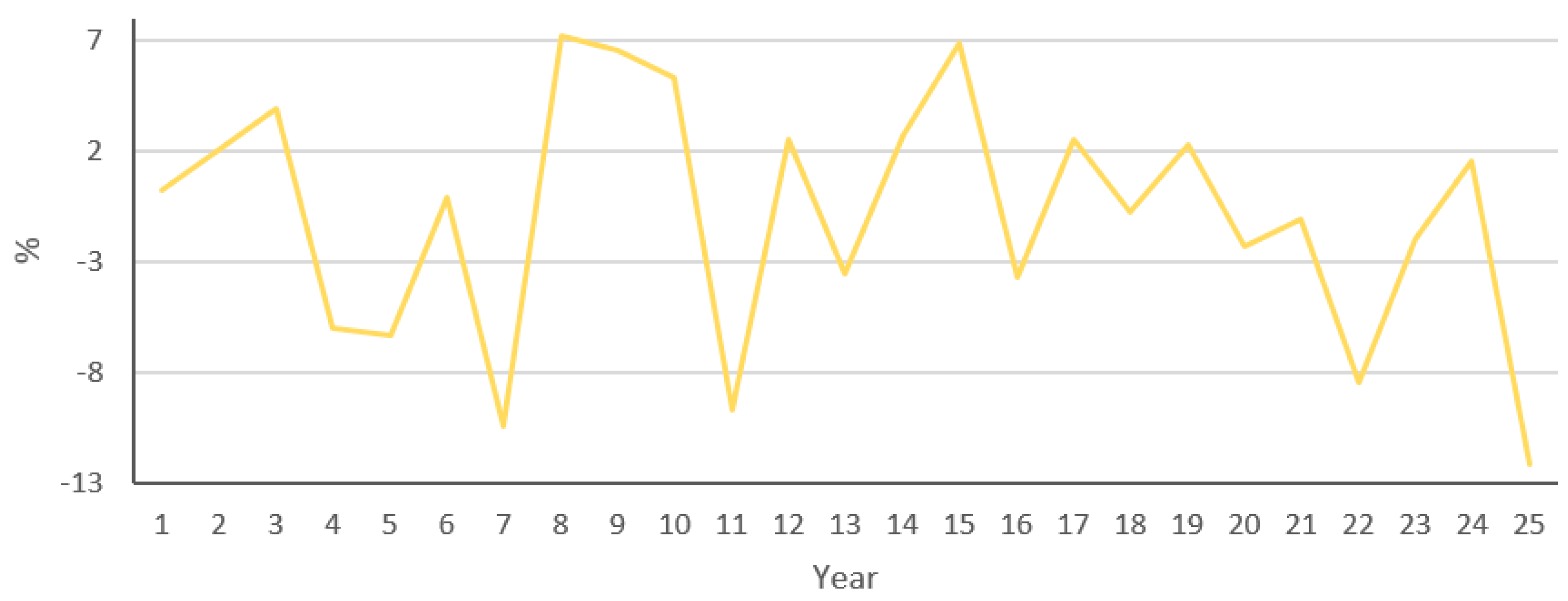
Figure 11.
Frequency of the first week of July.
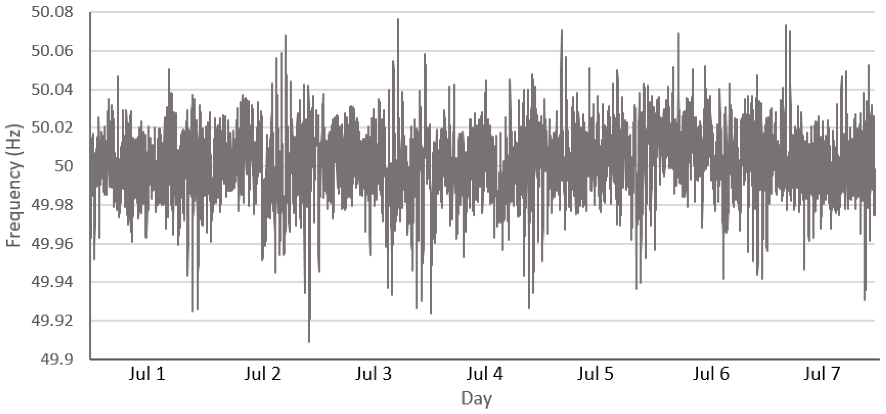
Figure 12.
FCR prices of the first week of July.
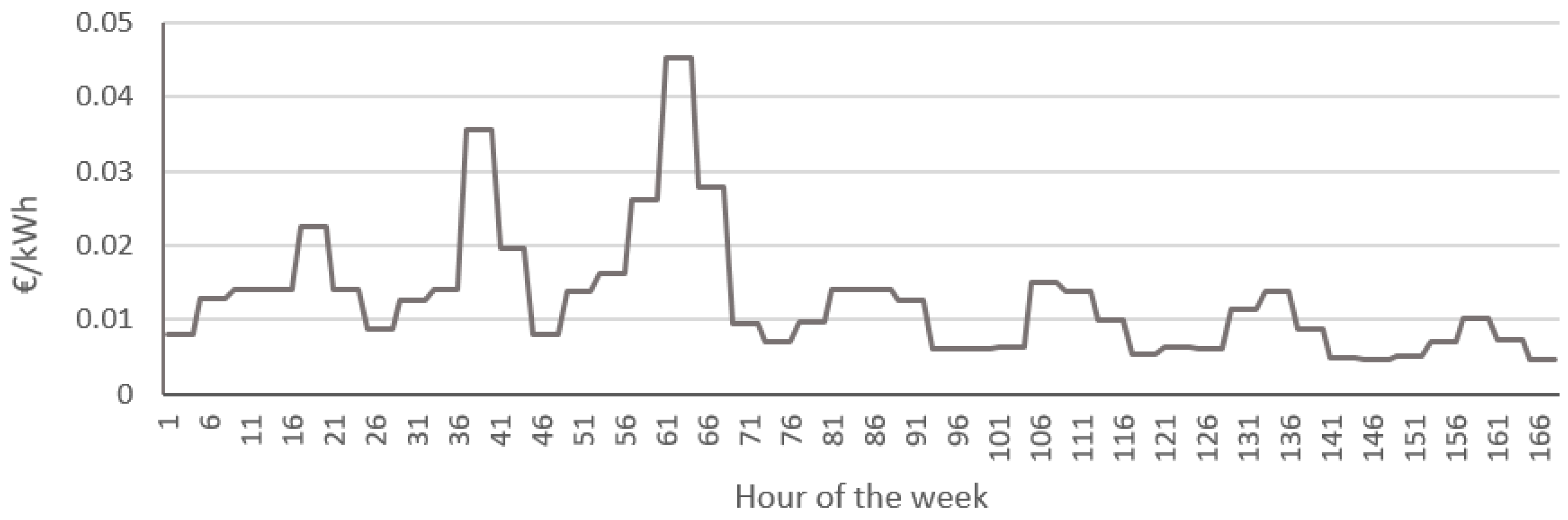
Figure 13.
Hourly electricity selling and purchasing price of the first year y.
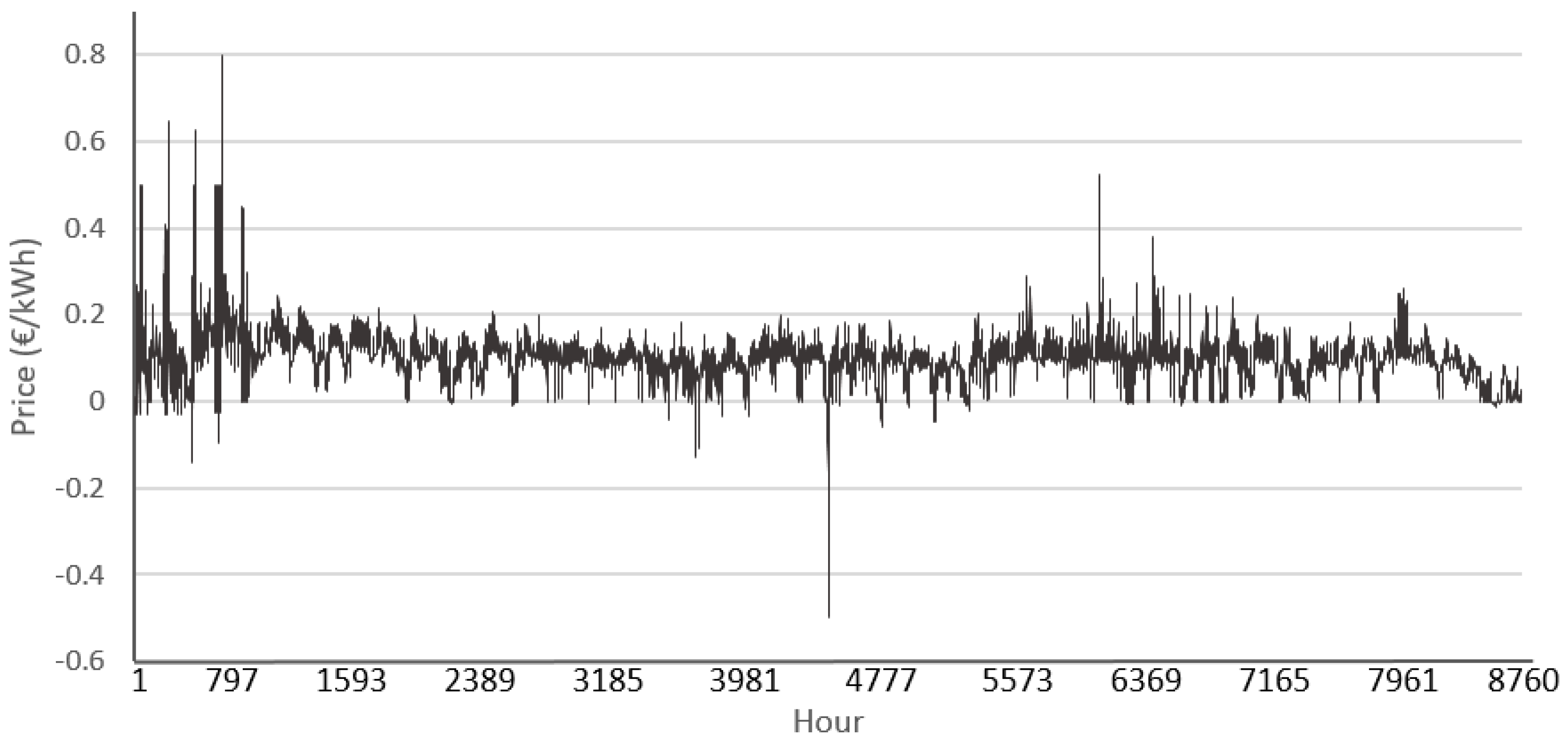
Figure 14.
Daily average hourly electricity selling price referred to the first year.
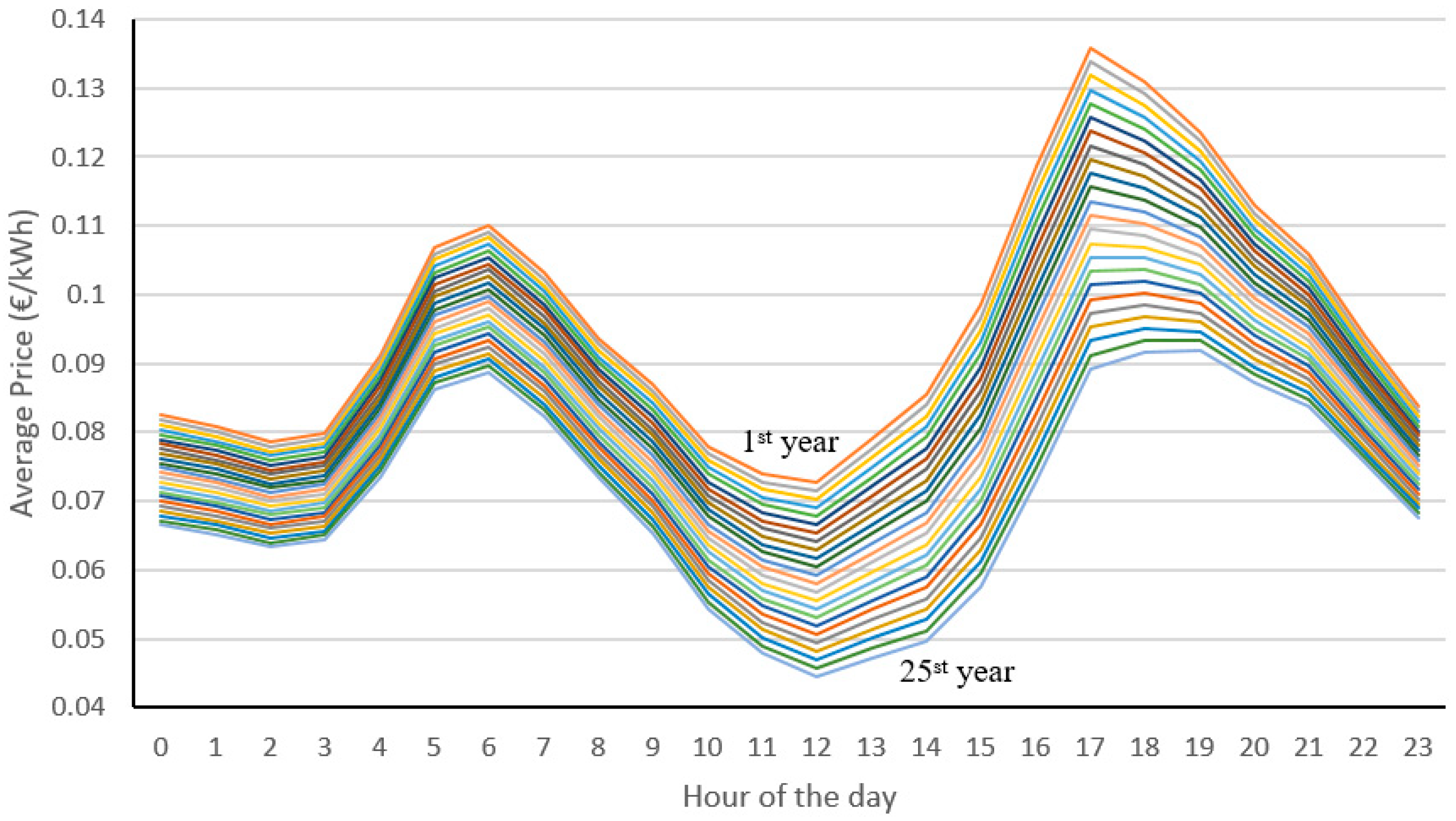
Figure 15.
Inverter efficiency.
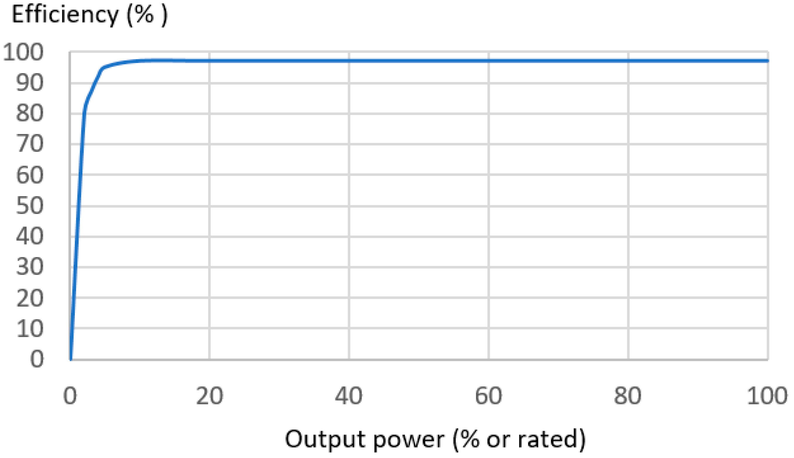
Figure 16.
Optimal AC-coupled system, simulation for two consecutive days.
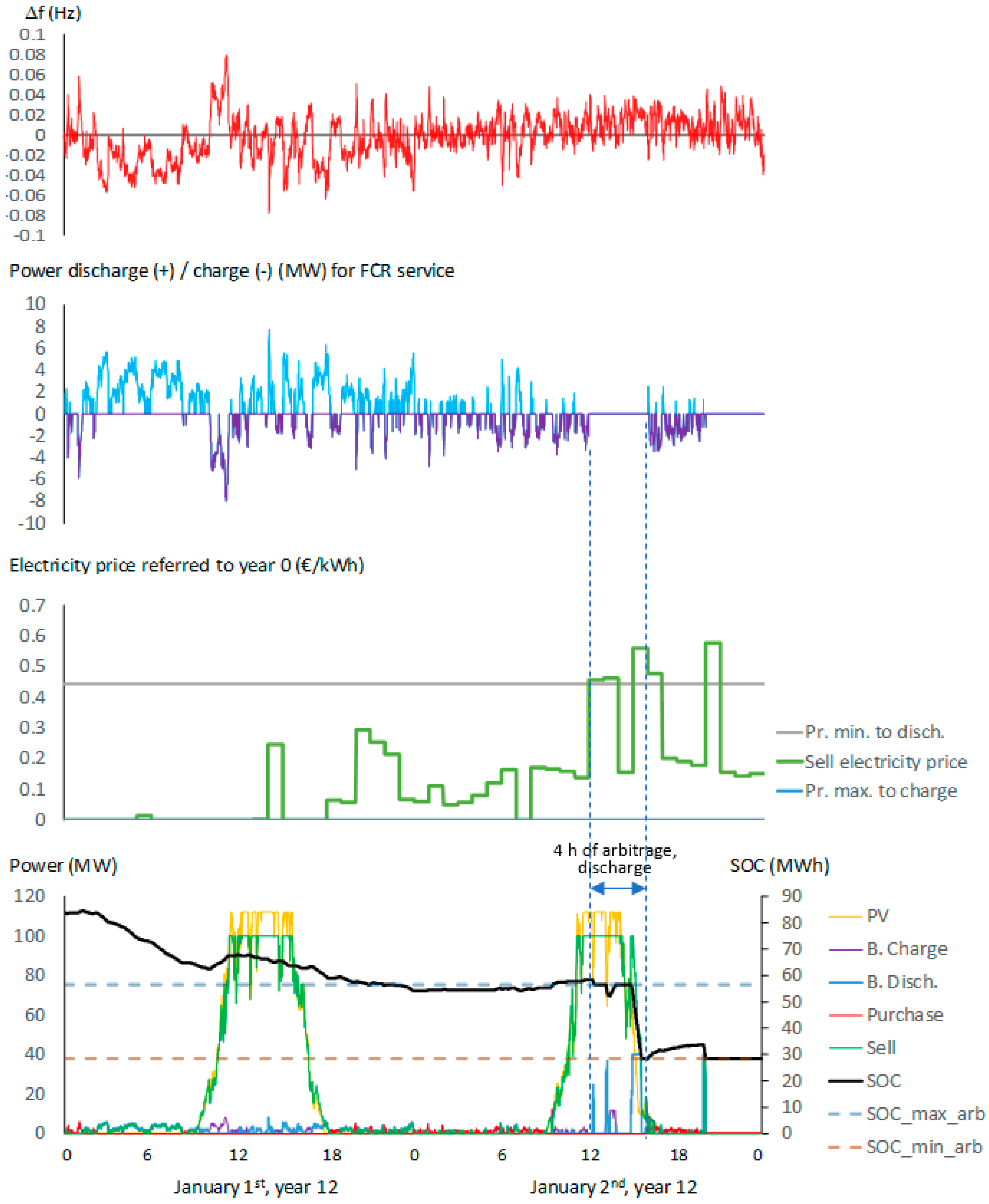
Figure 17.
Optimal DC-coupled system, simulation for two consecutive days.
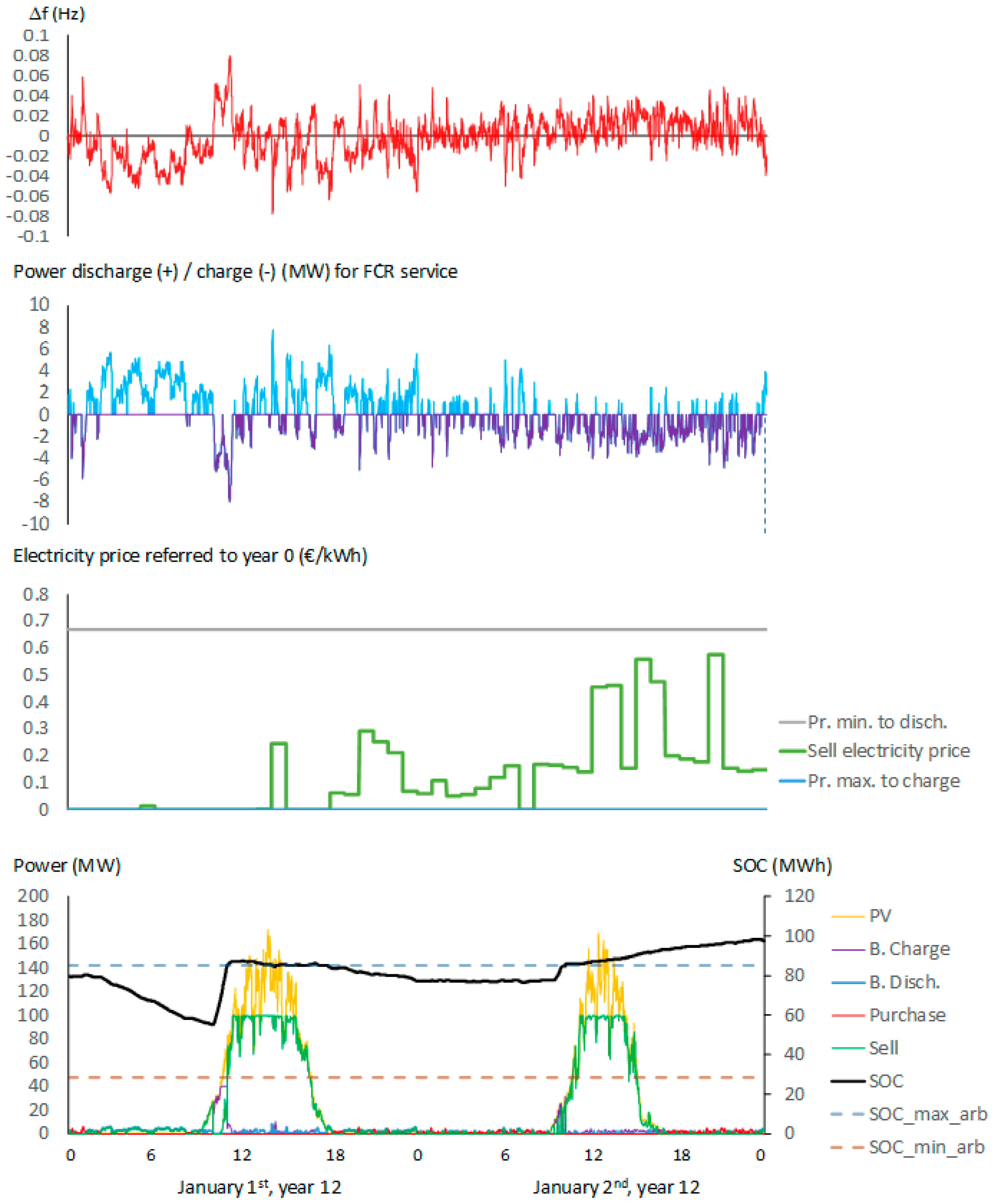
Figure 18.
Evolution of the GA and the PSO optimisations, AC-coupled system.
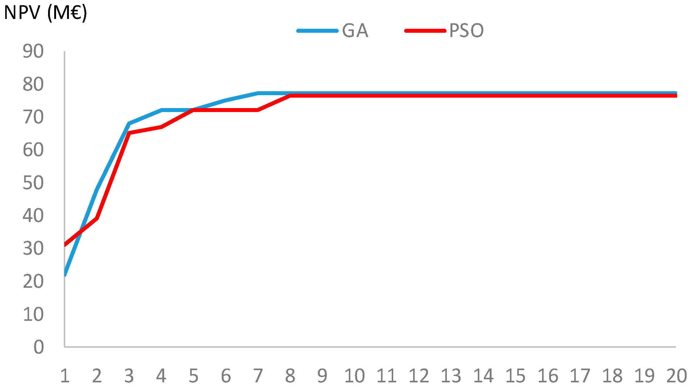

Table 1.
Data of the base case.
| Variable | Value | Variable | Value |
|---|---|---|---|
| Location | 50.70º N, 10.18º E | Inverter-charger: | |
| Resource data | PVGIS | CAPEX | 160 €/kW |
| 25 years | 40 MW to 100 MW | ||
| 100 MW | 10 years | ||
| 7% | Figure 13 [8] | ||
| 2% | 0.97 [8] | ||
| 1% | 0.982 [8] | ||
| PV (mono./bif.): | Li-ion LFP Battery: | ||
| AC coup. CAPEX | 0.54 / 0.5 €/Wdc | CAPEX | 295 €/kWh |
| DC coup. CAPEX | 0.5 / 0.46 €/Wdc | OPEX | 1% of CAPEX |
| OPEX | 1% of CAPEX | Cost escalation | -4%/yr |
| 80 to 160 MW | 160 MWh to 320 MWh | ||
| 0.5% [60] | 10% | ||
| 43ºC | 90% | ||
| 95% | /4 (4 h duration) | ||
| -0.4%/ºC | |||
| 0 / 0.7 | 1%/month | ||
| ILR (AC coupled) | 1.25 | 20% | |
| Figure 13 [8] | Ageing model parameters | [43], [44] |
Table 2.
Optimal systems for the base case. Comparison to the system without storage (PV-only).
| PV-plus-battery | PV-only | |||
|---|---|---|---|---|
| AC-coupled | DC-coupled | |||
| PV (MWdc) | 140 (7 x 20 MWdc), bifacial | 140 (7 x 20 MWdc), bifacial | 160 (8 x 20 MWdc), bifacial | |
| Battery (MWh) | 160 (4 x 40 MWh) | 160 (4 x 40 MWh) | - | |
| Battery max. power (MW) | 40 | 40 | ||
| Inverter-charger (MW) | 40 | 100 | - | |
| ILR | 1.25 (own inv.) | 1.4 | 1.25 (own inv.) | |
| BIR | 1 | 0.4 | - | |
| (€/kWh) | 0 | 0 | - | |
| (€/kWh) | 0.352 | 0.528 | - | |
| (% of max.) | 20 | 20 | - | |
| (% of max.) | 40 | 60 | - | |
| NPV (M€) | 77.35 | 60.28 | 121.05 M€ | |
| CAPEX (Invest. cost) (M€) | 129.2 | 133.2 | 86.4 | |
| Land use (ha) | 351.6 | 351.6 | 400 | |
| CF (%) | 21.29 | 20.72 | 22.63 | |
| IRR (%) | 12.9 | 10.15 | 20.77 | |
| LCOE (€/kWh) | 0.06 | 0.066 | 0.035 | |
| PV generation (GWh/yr) | 189.2 (AC) | 199.61 (DC) | 216.24 (AC) | |
| Batt. charge energy (GWh/yr) | 7.92 | 9.61 | - | |
| Batt. disch. energy (GWh/yr) | 7.12 | 8.64 | - | |
| Hours of bat. charge per year | 2725.6 | 2730.5 | - | |
| Hours of bat. disch. per year | 2693.8 | 2714.9 | - | |
| Battery lifetime (years) | 19.8 | 20.4→ 20 | - | |
| Sold energy (GWh/yr) | 186.46 | 181.52 | 198.22 | |
| Purchased energy (GWh/yr) | 3.57 | 3.44 | - | |
| Sell E. incomes (M€/yr) | 13.43 | 12.86 | 14.38 | |
| Sell E. incomes, NPV (M€) | 202.70 | 194.22 | 219.75 | |
| FCR serv. inc. (M€/yr) | 2.30 | 2.43 | - | |
| FCR serv. inc., NPV (M€) | 34.79 | 36.74 | - | |
| Purch. E. cost (M€/yr) | 0.32 | 0.31 | - | |
| Purchase E. cost, NPV (M€) | 4.69 | 4.54 | - | |
Table 3.
NPV variation over the base case (%) for cases of x_bool = 0, cases without FCR and cases of 1 h FCR service.
Table 3.
NPV variation over the base case (%) for cases of x_bool = 0, cases without FCR and cases of 1 h FCR service.
| AC-coupled | DC-coupled | |
|---|---|---|
| = 0 | -20.2% | -23.4% |
| No FCR | -25.4% | -44.8% |
| FCR service 1 h | 0.9% | 1.6% |
Table 4.
Battery lifetime (years) with or without FCR service.
| AC-coupled | DC-coupled | |
|---|---|---|
| With FCR | 19.8 | 20.4 → 20 |
| Without FCR | 20 | 21.9 → 20 |
Table 5.
NPV variation over the base case (%) for different electricity price annual inflation cases.
Table 5.
NPV variation over the base case (%) for different electricity price annual inflation cases.
| Electricity Price Inflation (%) | AC-coupled | DC-coupled |
|---|---|---|
| -2 | -93% | -109% |
| -1 | -73% | -87% |
| 0 | -52% | -61% |
| 1 | -27% | -36% |
Table 6.
NPV variation over the base case (%) for different cases of battery cost reduction.
| Battery price reduction (%) | AC-coupled | DC-coupled |
|---|---|---|
| 25% | 20% | 23% |
| 50% | 41% | 46% |
| 75% | 61% | 70% |
Table 7.
Optimal systems for the system located in Spain.
| PV-plus-battery | PV-only | |||
|---|---|---|---|---|
| AC-coupled | DC-coupled | |||
| PV (MWdc) | 140 (7 x 20 MWdc), bifacial | 140 (7 x 20 MWdc), bifacial | 160 (8 x 20 MWdc), bifacial | |
| Battery (MWh) | 160 (4 x 40 MWh) | 160 (4 x 40 MWh) | - | |
| Battery max. power (MW) | 40 | 40 | ||
| Inverter-charger (MW) | 40 | 100 | - | |
| ILR | 1.25 (own inv.) | 1.4 | 1.25 (own inv.) | |
| BIR | 1 | 0.4 | - | |
| (€/kWh) | 0.145 | 0.096 | - | |
| (€/kWh) | 0.242 | 0.242 | - | |
| (% of max.) | 30 | 40 | - | |
| (% of max.) | 60 | 60 | - | |
| NPV (M€) | 99.36 | 77.02 | 144.33 | |
Disclaimer/Publisher’s Note: The statements, opinions and data contained in all publications are solely those of the individual author(s) and contributor(s) and not of MDPI and/or the editor(s). MDPI and/or the editor(s) disclaim responsibility for any injury to people or property resulting from any ideas, methods, instructions or products referred to in the content. |
© 2024 by the authors. Licensee MDPI, Basel, Switzerland. This article is an open access article distributed under the terms and conditions of the Creative Commons Attribution (CC BY) license (http://creativecommons.org/licenses/by/4.0/).
Copyright: This open access article is published under a Creative Commons CC BY 4.0 license, which permit the free download, distribution, and reuse, provided that the author and preprint are cited in any reuse.


