
Submitted:
05 November 2024
Posted:
07 November 2024
You are already at the latest version
Abstract
Polyhedral cages (p-cages) describe the geometry of some families of artificial protein cages. We identify the p-cages made out of families of equivalent polygonal faces such that the faces of 1 family has 5 neighbours and P_1 edges, while those of the other family have 6 neighbours and P_2 edges. We restrict ourselves to polyhedral cages where the holes are adjacent to at most 4 faces. We characterise all the p-cages with a deformation of the faces, compared to regular polygons, not exceeding 10%.
Keywords:
Uniform Polyhedra
; Polyhedral Cages
; Platonic Group
; Near-miss Cages
; Cayley graph
; Protein Cage
; Nano-cage
; Capsid
; Nanoparticle
1. Introduction
A few years ago, J. Heddle created an artificial protein cage made out of 24 so-called rings themselves made out of 11 copies of the same protein called TRAP [1]. The nano-cage appears to be a regular structure made out of 24 hendecagons, with some small holes, which is mathematically impossible. It was shown that the faces of the corresponding structure are not regular but that the deformation of their edge lengths and angles is less than half a percent [2] making them look regular for the naked eye. These small deformations can easily be absorbed by the proteins and the termini where the faces are linked together. A small nano-cage made out of the same ring but counting only 12 of them was made in the same lab[3]. This was also identified as a nearly regular structure but one where the deformations are approximately 2.5%.
These discoveries led us to define polyhedral cages [4] (p-cages for short) as assemblies of polygons with holes, requiring that each face shares edges with at least 3 other faces and also imposing that of any two adjacent edges of a face only one of them can be shared. While the faces must be planar convex polygons, the holes can have any shape. In what follows, we only consider convex p-cages, as defined in [4,5].
P-cages are said to be regular if all the faces are regular and near-miss if they are slightly deformed. Homogeneous p-cages are made out of polygons with the same number of edges while bi-homogeneous p-cages are made out of 2 types of polygons. In [5] we defined symmetric p-cages as p-cages for which any two faces can be mapped into each other via a rotation which is an automorphism of the p-cage. Similarly, bi-symmetric p-cages are bi-homogeneous p-cages for which any 2 faces belonging to the same family can be mapped into each other via a rotation automorphism of the p-cage [6].
When we consider near-miss p-cages we must decide how large a deformation we are willing to consider. In [4,5] we have identified all regular and near-miss symmetric p-cages made out of polygons with up to 20 edges and with deformations not exceeding 10%. In [6] we have identified the bi-symmetric p-cages where each face of a given type are only sharing edges with faces of the other type, again restricting ourselves to 10% deformation and polygons with up to 20 edges.
The aim of this paper is to identify bi-symmetric p-cages where the faces have a maximum number of neighbours. As it is not possible for all the faces to have 6 neighbours [7], we consider p-cages for which the faces of the first type have 5 neighbours each while the faces of the second type have 6.
So far, a number of artificial protein cages have been experimentally generated [8,9,10,11,12,13]. The main aim is to develop new drug delivery methods [14,15,16,17,18]. The idea is to encapsulate the drug inside the cage while specific receptors are linked to the holes outside the cage to bind with the cells that are targeted such as cancer cells [14]. Once absorbed by cell, the protein-cage can release the drug in the cytoplasm [19]. This will lead to more efficient drug delivery as a smaller amount of the drug must be provided with the bonus of reduced side effects as only the targeted cells will be affected.
While the virus capsids found in nature are essentially based on the geometry of platonic solids [20] some of the cages created experimentally exhibit somewhat different structures [2,3,21]. It is then natural to ask the question as to what geometries are possible for such cages [22,23,24].
The aim of this paper is to find further potential geometries for nano-protein cages, identifying all bi-symmetric ones with maximal connectivity between the faces as well exhibiting small holes.
2. Methodology
As described in [4] to construct a p-cage one must first consider the planar graph obtained by joining the centres of the neighbouring faces of the p-cage with straight lines. We call the resulting object the hole polyhedron graph because its faces describe how many faces surround each hole. The nodes of the hole polyhedron graph correspond to the faces of the p-cage while the edges describe how the faces are joined together.
Our aim in this paper is to construct p-cages made out of 2 families of faces such that each face of a given family can be mapped by an automorphism rotation of the p-cage to any other face of the same family.
In what follows we define as the valency of a face the number of neighbour that it has. As we are interested by p-cages with the maximum number of neighbours, we impose that the faces belonging to the first family has valency 5 while the other faces valency 6. As we are interested only in p-cages with small holes we also impose that the faces of the hole polyhedron graphs are triangles, squares or any mix of each.
The naming convention of the graphs is described in [7] but the end of these names is particularly useful as in Vn_m, n and m correspond respectively to the numbers of pentavalent and hexavalent nodes and hence also correspond to the numbers of p-cage faces with 5 and 6 neighbours respectively.
In what follows, we denote by and the numbers of edges of the faces belonging to the families 1 and 2 respectively. When a polygon with P edges has n neighbours its has edges which must be distributed between the n edges adjacent to neighbour faces. If we use the labels a, b,c, d, e, to label the numbers of edges given to each hole by the first family of face and A, B,C, D, E, F for the second family, we have
for the faces belonging respectively to the first and the second family. We must then find out how distribute them on each of the identified hole polyhedron graphs in such a way that the equivalence between the faces is preserved. We now consider each of these 9 graphs one by one:
For HAP6 the corners of the valency 6 nodes must all be identical, but the corners around the valency 5 nodes can be arbitrary (Figure 1a).
For TTP6 the corners of the valency 6 nodes must be alternating A-B-A-B-A-B but then the corners of the valency 5 nodes can be arbitrary (Figure 1b).
For TOP6 the corners of the valency 5 nodes are arbitrary and mapped as in Figure 2a. The corners of the valency 6 nodes must then alternate between A and B (Figure 2a).
For PD the equivalence between two adjacent valency 6 nodes is achieved either via a 5-fold rotation around the pyramid or via a rotation around the centre of the link joining them. In either case we see that the corners around the valency 5 nodes must all be equal. Then the corners of the valency 6 nodes must be alternatingly A and B (Figure 2b).
For IP5 we see that by symmetry, the corners of the triangles joining the valency 6 nodes must all be the same so the corners of the valency 5 nodes are also all identical. Then for the valency 6 nodes we have the sequence A-B-C-A-B-C (Figure 3a).
For SDP50 the corners around the valency 5 nodes must all be the same but then the corners around the valency 6 nodes are arbitrary as shown in the figure (Figure 3b).
The p-cages TTM3 and TOM3 do not lead to any p-cages with deformations below 10% and the best TCM3 p-cages having deformations exceeding 8% are not good candidates for protein cages as the faces are too irregular for proteins rings to adjust to the deformations. For this reason the construction of these 3 families of cages is described in the supplementary material.
To construct the p-cages we follow a method similar to the one described in [5,6]: we derive the most general parametrisation for the different faces which we then use to determine numerically the faces which are least irregular.
First we notice that each of the identified hole polyhedron graphs are built from an Archimedean solid, the dual of an Archimedean solid or an antiprism. Given a face of any of the 2 families, all the other faces of the same family will be obtained by applying the symmetry of the regular solid underlying the hole polyhedron graph. We label each face with its family type j, set to 1 for the pentavalent faces and 2 for the hexavalent faces, as well as an index number i. Each face will belong to a plane plane going through the vector and spanned by the orthonormal basis vector and . We also chose such that it is orthogonal to the considered plane. The planes and faces with index are called the reference plane and face respectively. The remaining faces of the p-cage can then be obtained by applying a rotation to the reference faces. We can then determine the lines of intersection between adjacent faces knowing that the shared edges will lie on these lines. The vertices of the reference faces can then be parametrised in the reference plane restricting the vertices belonging to two faces to lie on the corresponding intersection lines. The vertices belonging to a hole will belong to the reference plane without any further restriction.
We then have to identify the face configuration for which the faces are as regular as possible.
First we denote , , the vertices of a face, ordered anticlockwise when seen from outside the p-cage and the normal to the reference face of type j pointing out of the p-cage. We then define the edge vector so that the edge lengths are given by and compute the angle between adjacent edges, by evaluating and
Notice that in (2) corresponds to the angle inside the face which is larger than if the face is not convex. For a regular P-polygon, .
After computing the and we can minimise the deviation from the regularity energy
where
with the 3 weight factors , and . , given explicitly by
where is the Heaviside function. (5), is 0 unless the polygon defined by the vertices is concave.
To compute we find , the position of the centre of face i and if we consider 2 adjacent faces and with normal vectors and respectively. The p-cage is convex by if for all pairs of adjacent faces, the distance between the centres of the 2 faces is smaller than the distance between and . This is used to define as
where is the set of faces, of any type, adjacent to the reference face j. Notice that is 0 unless the p-cage is concave.
These last two terms are used in the simulated annealing optimisation procedure to enforce convexity of the faces and the p-cage by taking large values for and . In (3) we divide the sum by to make the parametrisation of the optimising algorithm easier.
3. Notation
In what follows we denote with a rotation of angle around the vector . We also denote , and the rotation of an angle around the respective axis x, y and z.
The plane of face can be parametrised using the point contained in the plane and the plane basis vectors and as
Given two such planes with parametrisation and we must find the intersecting line which determines where the edge shared by the two adjacent faces is. First we define the normal vectors to each planes, and , as well as the vector parallel to the plane intersection:
Any point on that line is in the range of the parametrisations of both planes:
If that point is perpendicular to then a relation holds among , and , , obtained by multiplying both sides of (9) by which, as detailed in [25], when inserted back into (9) gives
To obtain the intersection point of 2 coplanar lines, and where we assume and to be normalised to 1, we need to find the value of so that
Multiplying (11) by respectively and we obtain
Substituting the second equation in the first one we obtain for the point of intersection
In what follows, will denote the intersection point between the following 3 faces: the reference face of type 1, the face i of type and the face k, of type . This corresponds to the intersection point between the two lines and obtained using (13). Similarly will denote the intersection point between the reference face of type 2, the face i of type and the face k of type .
To denote face i of type j we use the notation and each face with index is related to the references face of the correct type via a rotation
The spanning vectors , and will then be obtained via the same rotation:
4. Parametrisation
4.1. HAP6
The symmetry of the HAP6 p-cage is that of the hexagonal anti-prism. For the reference face vectors we have choose the following:
and the rotations between the faces are
where is an angle which allows the top and bottom halves of the p-cages to be shifted sideways with respect to each others.
Figure 4.
Parametrisation of the hexagonal antiprism p-cage.
The nodes of the reference face of type 1 shared with the adjacent faces are
for some parameters . The nodes of the reference face of type 2 are then given by
The optimization parameters are , , , , , , , , , as well as the coordinates of the non-shared vertices within the plane of the faces for both reference faces.
For the optimisation to work well it helps to start from a reasonable initial configuration. We notice that the 10 shared edges between the reference face and its 5 neighbours form a pentagon and we can easily determine the coordinates of its vertices. As an initial configuration we can locate the shared vertices so that the edges of the pentagon are split in 3 equal parts. The unshared vertices can then be be placed equally spaced between these vertices. This is done explicitly in the code supplied on Zenodo. For the other parameters, we choose as initial values , and .
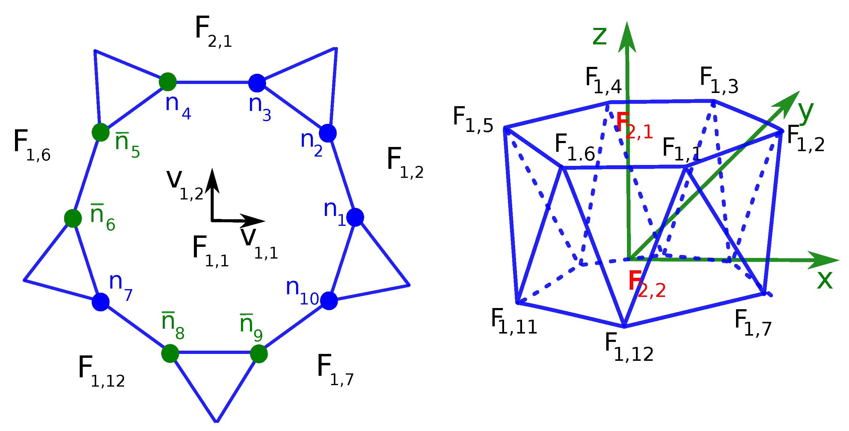
4.2. TTP6
The underlying symmetry of the TTP6 p-cage is that of the truncated tetrahedron. We have oriented the tetrahedron as depicted in Figure 5.
The coordinates of the vertices of the centred tetrahedron are
while the centres of the reference faces are given by
and the rotations linking the faces are
We choese the following vectors to parametrise the reference planes:
where and are scaling parameters. The shared vertices of the reference faces are then given by
The optimization parameters are , , , , , , , , , , as well as the planar coordinates of the non-shared vertices for both reference faces. As initial parameter values we have used , and , . The other parameters are determined as described in the HAP6 section.
4.3. TOP6
The underlying symmetry of the TOP6 p-cage is that of the truncated octahedron. We orient the octahedron as depicted in Figure 6.
For the vectors normal to the reference faces we use
and the rotations linking the faces to the reference faces are
We choose the following vectors to parametrise the reference plane:
where and are scaling parameters.
The shared vertices of the reference faces are then given by
The optimization parameters are , , , , , , , , , , as well as the planar coordinates of the non-shared vertices for both reference faces. As initial parameter values we choose , and . The other parameters are determined as described in the HAP6 section.
4.4. PD
The underlying symmetry of the PD p-cage is that of the dual of the truncated icosahedron. The pentagons sit on the vertices of the icosahedron while the hexagon areplaced at the centres of the triangular faces of the icosahedron.
The coordinates of the icosahedron are given by the coordinates of 3 perpendicular golden ratio rectangles
where is the golden ratio. The type 1 faces are placed on the vertices of the icosahedron while the type 2 faces are placed at the centre of the icosahedron faces
Defining
the rotations linking the faces to the reference faces are
We choose the following vectors to parametrise the reference plane:
where and are scaling parameters.
The shared vertices of the reference faces are given by
The optimization parameters are , , , , , as well as the planar coordinates of the non-shared vertices for both reference faces. As initial parameters values we choose , while the other parameters are determined as described in the HAP6 section.
4.5. IP5
The underlying symmetry of the IP5 p-cage is that of the dual of the icosidodecahedron.
Figure 8.
Parametrisation of the icosidodecahedron with a pyramid on the pentagonal faces p-cage. a) Icosidodecahedron vectors. b) Mapping of vertices.
Figure 8.
Parametrisation of the icosidodecahedron with a pyramid on the pentagonal faces p-cage. a) Icosidodecahedron vectors. b) Mapping of vertices.
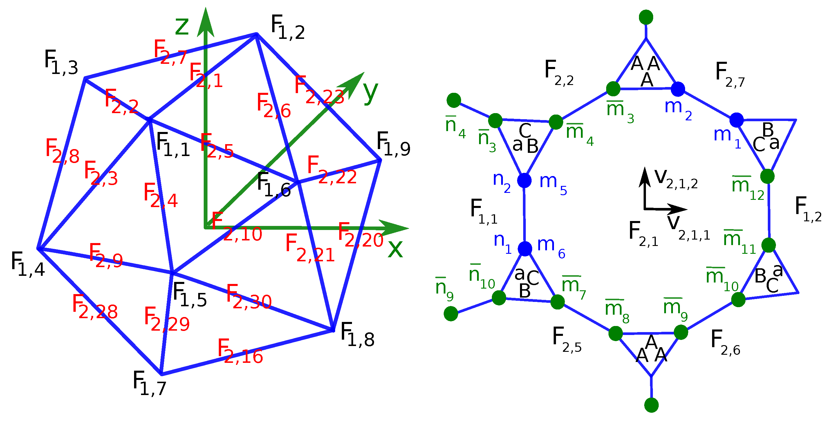
The type 1 faces are placed at the centres of the pentagons of the icosidodecahedron. The vectors pointing to these centres correspond to the 12 vertices of the icosahedron. The type 2 hexagonal faces are placed on the vertices of the icosidodecahedron which correspond to the midpoint of icosidodecahedron edges:
The rotations linking the faces to the reference faces are
where and
We choose the following vectors to parametrise the reference plane:
where and are scaling parameters.
The shared vertices of the reference faces are given by
The optimization parameters are , , , , , as well as the planar coordinates of the non-shared vertices for both reference faces. As initial parameters values we choose , while the other parameters are determined as described in the HAP6 section.
4.6. SDP5
The underlying symmetry of that of the SDP5 p-cage is that of the snub dodecahedron.
Figure 9.
Parametrisation of the cage built on a snub dodecahedron with pyramids on the pentagons p-cage. a) Dodecahedron node numbering. b) Face labelling. The green dots correspond to the vectors c) Mapping of vertices.
Figure 9.
Parametrisation of the cage built on a snub dodecahedron with pyramids on the pentagons p-cage. a) Dodecahedron node numbering. b) Face labelling. The green dots correspond to the vectors c) Mapping of vertices.
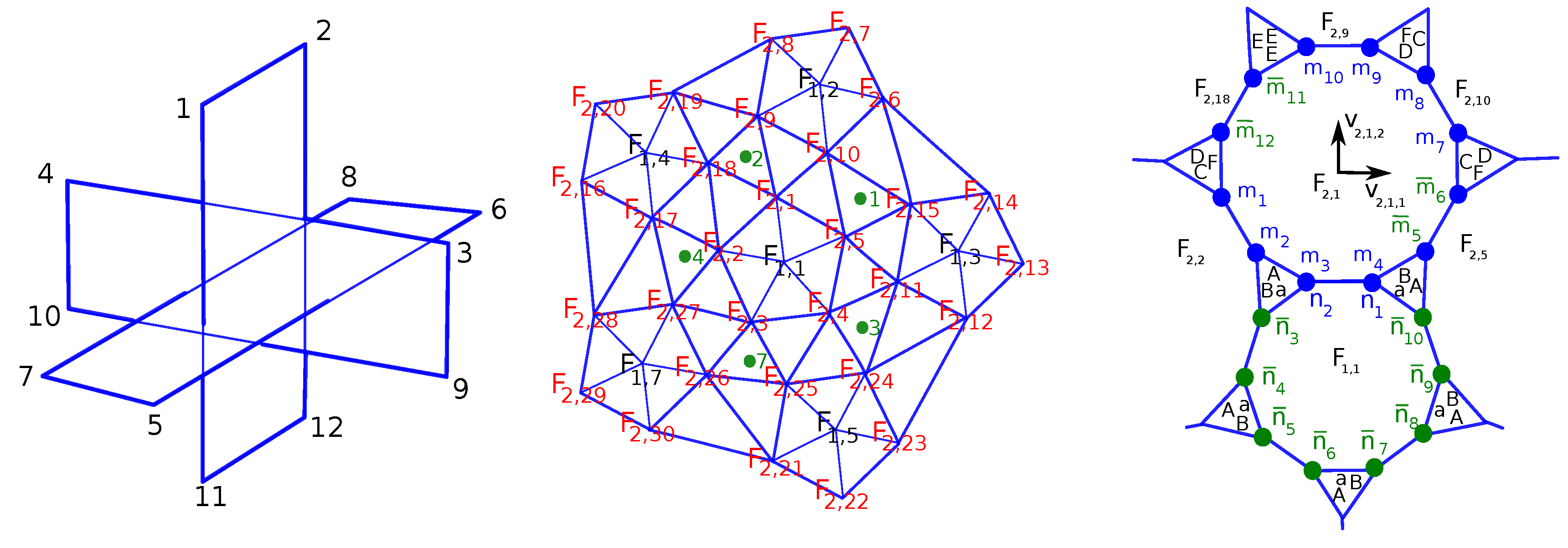
The normal vectors to the reference planes are
Defining , the rotation axe vectors are
The rotations linking the faces to the reference faces are given by
We choose the following vectors to parametrise the reference plane:
With these we have
The optimization parameters are , , , , , , , , , ,, as well as the planar coordinates of the non-shared vertices for both reference faces. As initial parameter values we use , , , while the other parameters are determined as described in the HAP6 section.
5. Results
We used a computer program to optimise (3) for each configuration described above with the restrictions that each face contributes up to 3 of its edges to each hole. That restriction was chosen to avoid p-cages with very large holes. A python program was used to generate all the combinations of the labels a to e and A to F satisfying (1) where each label may take the values 1, 2 or 3 which led to over half a million configurations to optimize. We used a simulated annealing method to minimize (3) for 200 values of and , with the constraint , taking and the selected the p-cage with the smalest value of max().
The p-cages are named according to the graphs they are build from, the size of the face and the number of edges contributing to the holes as follows : GRAPH_P_P_a_b_c_d_e-A_B_C_D_E_F where the italic symbols are replaced by their value. To avoid very long names, we also use a simplification when n successive hole-edge labels have the same values, , where we replace the sequence by nx. So for example, IP5_P10_P12_5x1-6x1 is equivalent to IP5_P10_P12_1_1_1_1_1-1_1_1_1_1_1 or SDP5_P15_P21_5x2-2x2_2x3_2_3 is equivalent to SDP5_P15_P21_2_2_2_2_2-2_2_3_3_2_3.
Our first result was that none of these configurations led to regular p-cages. The best HAP6 p-cage has a deformation just under under 5%. The two type 2 faces, at the top and bottom of the p-cage, are surrounded by two rings of 5 type 1 faces joined together (Figure 10a).
The least deformed p-cages are of the type PD: PD_P20_P24_5x3-6x3 has deformations , and PD_P10_P12_5x1-6x1 which is similar in structure but with smaller polygons has deformations just exceeding 1%: , (Figure 10b–d).
The IP5 p-cages are made out of respectively 12 and 36 faces of type 1 and 2. The p-cages IP5_P10_P12_5x1-6x1 is nearly regular with deformations , . (Figure 10e).
The p-cage IP5_P10_P14_5x1-2_2x1_2_2x1 is interesting in that its hole-edge labels are not identical and still has relatively small deformations , (Figure 10f). The TOP6 p-cages are made out of respectively 24 and 8 faces of type 1 and 2. The p-cage TOP6_P11_P12_2_4x1-6x1 is particularly interesting in that it is made out of the polygons, hendecagons and dodecagons, from which the nano-cages used, separately, in [2,3] are made. Its deformations are relatively small too , (Figure 10g). The p-cage TOP6_P16_P18_3_4x2-6x2 is another example of a p-cage with differing hole-edge labels and with still relatively small deformations: , (Figure 10h).
The TTP6 p-cages are made out of respectively 12 and 4 faces of type 1 and 2. The p-cages TTP6_P20_P24_5x3-6x3, TTP6_P15_P18_5x2-6x2 and TTP6_P10_P12_5x1-6x1 all have a similar structure with respective deformations , , , and , (Figure 11a–c).
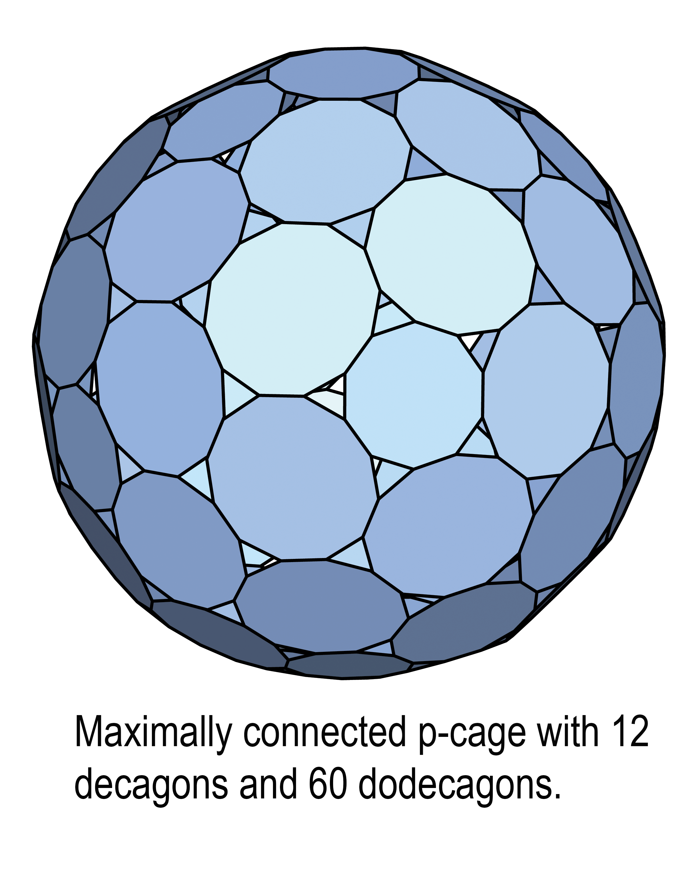
The SDP5 p-cages are made out of respectively 12 and 60 faces of type 1 and 2. These are the largest bi-symmetric p-cages with maximal connectivity between faces. The p-cages SDP5_P20_P24_5x3-6x3, SDP5_P15_P18_5x2-6x2 and SDP5_P10_P12_5x1-6x1 have a similar structure with deformations respectively , , , and , (Figure 11d,f,g). The p-cage SDP5_P15_P21_5x2-2x2_2x3_2_3 is another example of a p-cage with non identical hole-edge numbers and relatively small deformations , (Figure 11e).
The TCM4 p-cages are made out of respectively 24 faces of each type. The configuration TCM3 lead to 68 p-cages with deformation below 10% but the least deformed p-cage, TCM4_P20_P24_5x3-6x3, has a deformation of over 8%: , (Figure 11h ). While aesthetically pleasing, it does not constitute a good candidate for a protein cage.
6. Conclusion
In this paper we have constructed near-miss p-cages made out of two types of faces such that the faces of one family have 5 neighbours while the others have 6. Moreover each face of a given family can be mapped to any other face of the same family via a rotation automorphism of the p-cage.
We have shown that the p-cages can be constructed by placing the faces on the vertices of the so called hole-polyhedron, the edges of which describes how the faces are attached to each others. The bi-symmetry of the p-cage and the constraint of each face having 5 or 6 neighbours restricts the hole-polyhedron graphs to be one of 9 graphs identified in [7]. From these 9 hole-polyhedron graphs 2 leads to p-cages with deformation exceeding 10% (TTM3 and TOM3 p-cages) while the TCM3 p-cages have quite large deformations exceeding 8%. The other 6 types of p-cages have much smaller deformations, a number of them being approximately .
If we restrict ourselves to small P, so to a small number of hole-edges, the following p-cages are good candidates for artificial protein cages: PD_P10_P12_5x1-6x1 (deformation ), TOP6_P11_P12_2_4x1-6x1 (deformation ), IP5_P10_P12_5x1-6x1 (deformation ), TTP6_P10_P12_5x1-6x1 (deformation ), IP5_P10_P14_5x2-2_2x1_2_2x1 (deformation ) or SDP5_P10_P24_5x1-6x1 (deformation ). So each type of p-cage, except possibly HAP6, are potential geometries for good p-cages. Notice that SDP5_P10_P24_5x1-6x1 is the largest of such p-cages as it is made out of 72 faces. The TTP6 p-cages are the smallest with only 16 faces, while the TOP6 and PD p-cages have 32 faces while the IP5 p-cages have 42.
Supplementary Materials
The following supporting information is available in the supplementary material section:
- ExtraGraphsPcages.pdf : derivation of the 3 families of p-cages wich all exhibit large deformations.
- bi_symmetrix_full_list_56_34.pdf: full list, including figures, of all the p-cages with deformations not exceeding 10%.
- BestOFF.tar.gz: Coordinates of the best p-cages with deformations under 10% as off files.
Author Contributions
BP initiated the problem and established the methodology to characterise all the Polyhedral Cages with maximally connected faces. BP wrote the C++ code to construct all the p-cages, ran the code on the Condor cluster and analysed the results. AL checked the geometry of of the p-cages and the figures. The paper was drafted by BP. Both authors reviewed, amended and agreed to the final manuscript.
Funding
The research was funded by the Leverhulme Trust Research Project Grants RPG-2020-306.
Data Availability Statement
The C++ and Python programs used to generate all the data are available from https://zenodo.org/records/12805087[doi:10.5281/zenodo.12805087]
Acknowledgments
The computer simulations were performed on the Condor cluster of the Mathematical Science Department of Durham University. The figures were produced with the Geomview Software (http://www.geomview.org/) and the Inkscape Software (https://inkscape.org).
Abbreviations
| TRAP | trp RNA-binding attenuation protein. |
| RNA | Ribonucleic acid: a nucleic acid present in all living cells. |
| DNA | Deoxyribonucleic acid: a nucleic acid present in all living cells. |
References
- Malay, AD.; et al. Gold nanoparticle-induced formation of artificial protein capsids. Nano Lett. 2012, 12, 2056–2059. [Google Scholar] [CrossRef] [PubMed]
- Malay, AD.; Miyazaki, N.; Biela, A. et al. An ultra-stable gold-coordinated protein cage displaying reversible assembly. Nature, 2019; 569, 438–442. [Google Scholar] [CrossRef]
- Majsterkiewicz, K.; et al. Artificial Protein Cage with Unusual Geometry and Regularly Embedded Gold Nanoparticles. Nano Lett. 2022, 22, 3187–3195. [Google Scholar] [CrossRef] [PubMed]
- Piette, B.M.A. G; Kowalczyk A.; and Heddle J.G. Characterization of near-miss connectivity-invariant homogeneous convex polyhedral cages. Proc. R. Soc. A. 2021; 478, 20210679. [Google Scholar] [CrossRef]
- Piette, B.M.A. G; and Lukács A. Symmetry, 2023; 15, 717. [Google Scholar] [CrossRef]
- Piette, B.M.A. G; and Lukács A. Symmetry, 2023; 15, 1804. [Google Scholar] [CrossRef]
- Piette BMAG. Biequivalent Planar Graphs. Axioms 2024, 13, 437. [Google Scholar] [CrossRef]
- Chakraborti S, Lin TY, Glatt S, Heddle JG. Enzyme encapsulation by protein cages. RSC Adv. 2020; 10, 13293–13301. [CrossRef]
- A prototype protein nanocage minimized from carboxysomes with gated oxygen permeability Gao R, Tan H, Li S, Ma S, Tang Y, Zhang K, Zhang Z, Fan Q, Yang J, Zhang XE, Li F. A prototype protein nanocage minimized from carboxysomes with gated oxygen permeability. Proc Natl Acad Sci U S A. 2022; 119, e2104964119. [CrossRef]
- Zhu J, Avakyan N, Kakkis A, Hoffnagle AM, Han K, Li Y, Zhang Z, Choi TS, Na Y, Yu CJ, Tezcan FA. Protein Assembly by Design. PChem Rev. 2021; 121, 13701–13796. [CrossRef]
- Lapenta F, Aupič J, Vezzoli M, Strmšek Ž, Da Vela S, Svergun DI, Carazo JM, Melero R, Jerala R. Self-assembly and regulation of protein cages from pre-organised coiled-coil modules. Nat Commun. 2021; 12, 939. [CrossRef]
- Percastegui EG, Ronson TK, Nitschke JR. Design and Applications of Water-Soluble Coordination Cages. Chem Rev. 2020; 120, 13480–13544. [CrossRef]
- Golub E, Subramanian RH, Esselborn J, Alberstein RG, Bailey JB, Chiong JA, Yan X, Booth T, Baker TS, Tezcan FA. Constructing protein polyhedra via orthogonal chemical interactions. Nature. 2020; 578, 172–176. [CrossRef]
- Liang Y, Furukawa H, Sakamoto K, Inaba H, Matsuura K. Anticancer Activity of Reconstituted Ribonuclease S-Decorated Artificial Viral Capsid. Chembiochem. 2022; 23, e202200220. [CrossRef]
- Olshefsky A, Richardson C, Pun SH, King NP. Engineering Self-Assembling Protein Nanoparticles for Therapeutic Delivery. Bioconjug Chem. 2022; 33, 2018–2034. [CrossRef]
- Luo X, Liu J. Ultrasmall Luminescent Metal Nanoparticles: Surface Engineering Strategies for Biological Targeting and Imaging. Adv Sci (Weinh). 2022; 9, e2103971. [CrossRef]
- Naskalska A, Borzęcka-Solarz K, Różycki J, Stupka I, Bochenek M, Pyza E, Heddle JG. Artificial Protein Cage Delivers Active Protein Cargos to the Cell Interior. Biomacromolecules. 2022; 22, 4146–4154. [CrossRef]
- Edwardson TGW, Tetter S, Hilvert D. Two-tier supramolecular encapsulation of small molecules in a protein cage. Nat Commun. 2020; 11, 5410. [CrossRef]
- Stupka I, Azuma Y, Biela AP, Imamura M, Scheuring S, Pyza E, Woźnicka O, Maskell DP, Heddle JG. Chemically induced protein cage assembly with programmable opening and cargo release. Sci Adv. 2022; 8, eabj9424. [CrossRef]
- Twarock R, Luque A. Structural puzzles in virology solved with an overarching icosahedral design principle. Nat Commun. 2019; 10, 4414. [CrossRef]
- Sharma, A.P.; Biela, A.P.; et al. Shape-morphing of an artificial protein cage with unusual geometry induced by a single amino acid change. ACS Nanoscience Au, 2022; 2, 504–413. [Google Scholar]
- McTernan CT, Davies JA, Nitschke JR. Beyond Platonic: How to Build Metal-Organic Polyhedra Capable of Binding Low-Symmetry, Information-Rich Molecular Cargoes. Chem Rev. 2022; 123, 10393–10437. [CrossRef]
- Khmelinskaia A, Wargacki A, King NP. Structure-based design of novel polyhedral protein nanomaterials. Curr Opin Microbiol. 2021; 61, 51–57. [CrossRef]
- Laniado J, Yeates TO. A complete rule set for designing symmetry combination materials from protein molecules. Proc Natl Acad Sci U S A. 2020; 117, 31817–31823. [CrossRef]
- Coxeter, H.S.M. Regular polytopes. Dover Publications, Mineola, NY, USA, 1973.
Figure 1.
Hole-edges mapping for the hole polyhedron graphs: a) HAP6 b) TTP6.
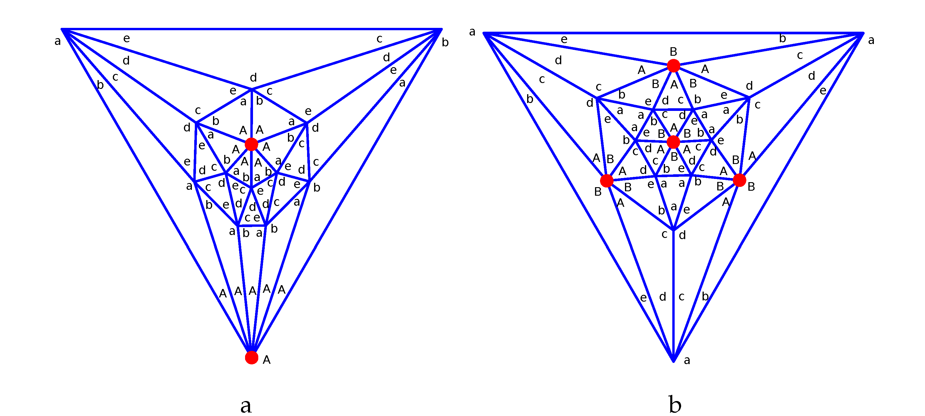
Figure 2.
Hole-edges mapping for the hole polyhedron graphs: a) TOP6 b) PD.
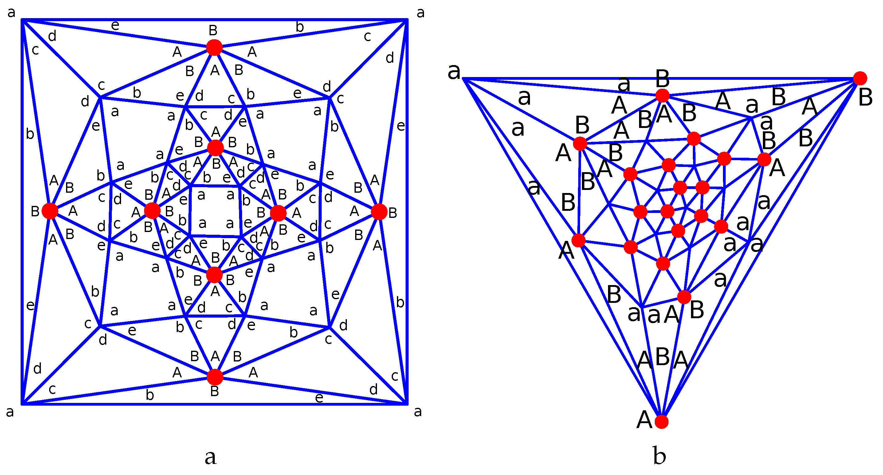
Figure 3.
Hole-edges mapping for the hole polyhedron graphs: a) IP5 b) SDP5.
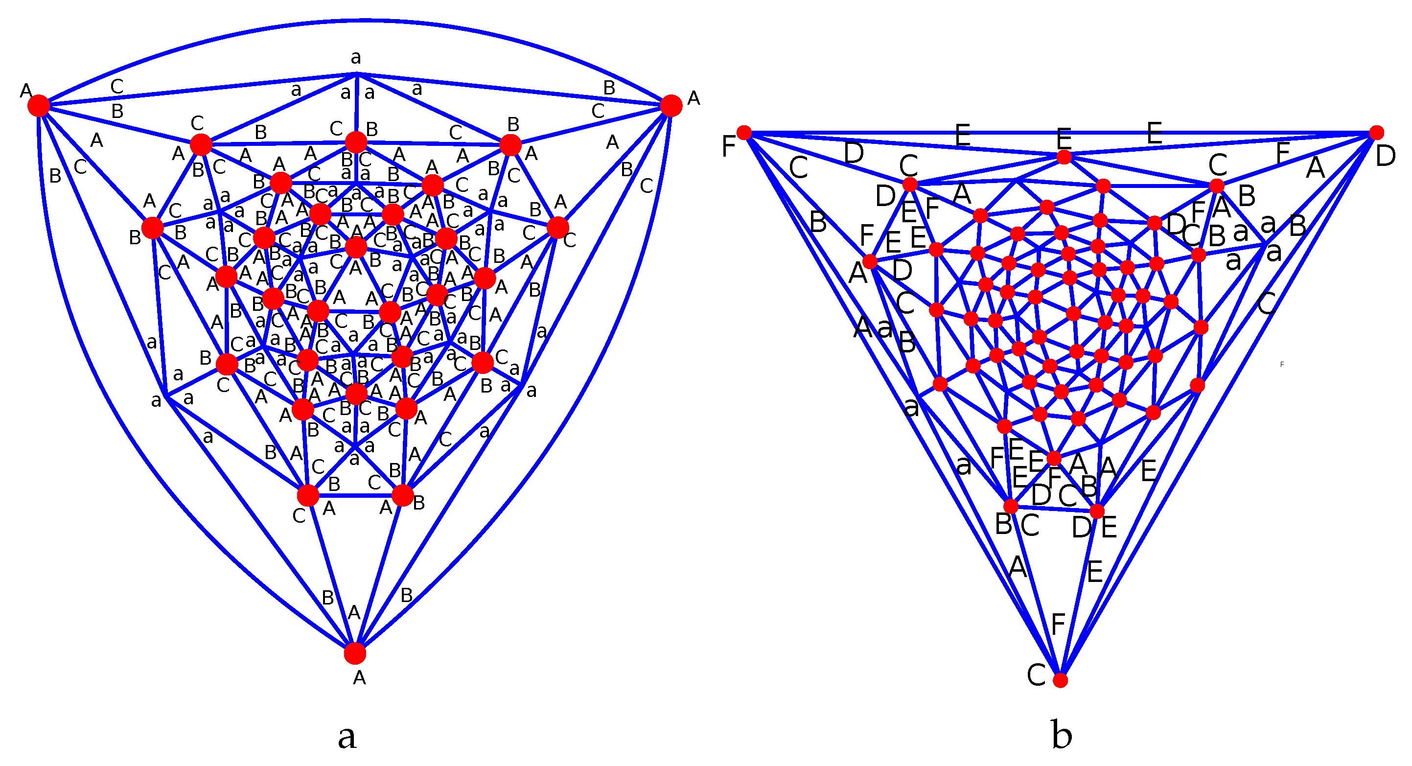
Figure 5.
Parametrisation of the truncated tetrahedron TTP6 p-cage. a) Truncated tetrahedron vectors. b) Mapping of vertices.
Figure 5.
Parametrisation of the truncated tetrahedron TTP6 p-cage. a) Truncated tetrahedron vectors. b) Mapping of vertices.
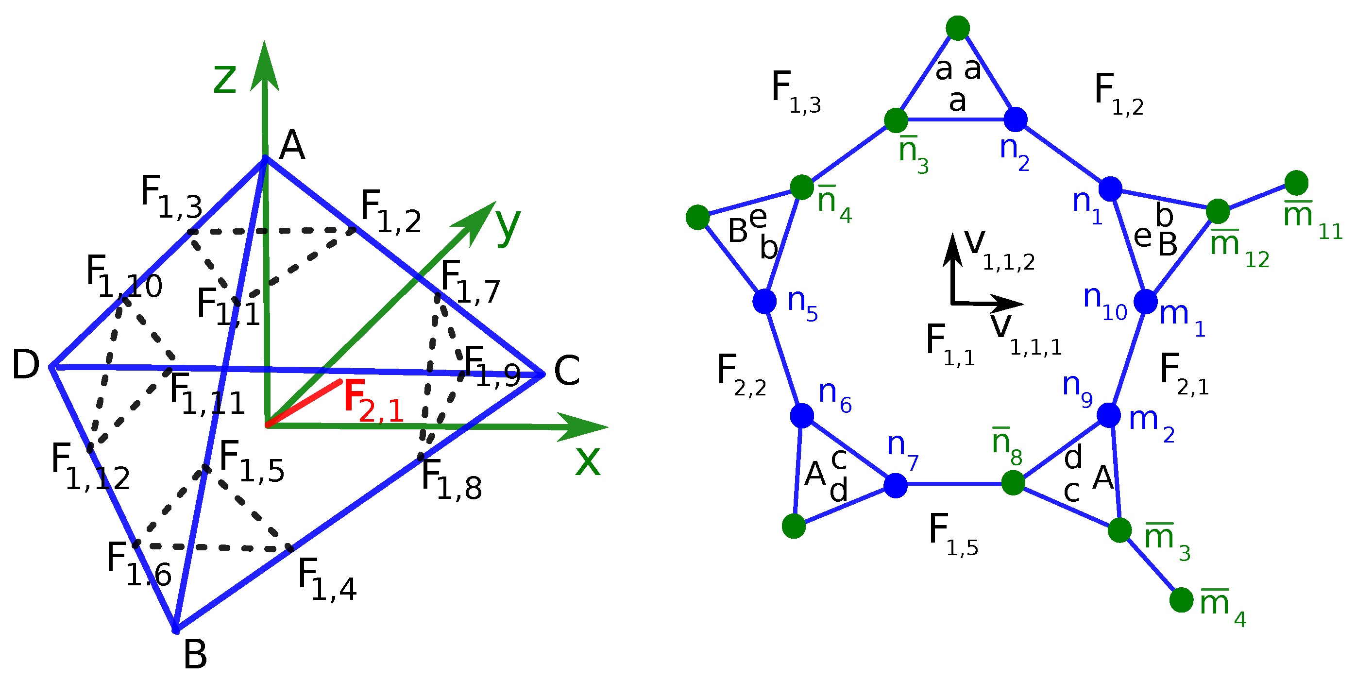
Figure 6.
Parametrisation of the truncated tetrahedron TOP6 p-cage. a) Truncated tetrahedron vectors. b) Mapping of vertices.
Figure 6.
Parametrisation of the truncated tetrahedron TOP6 p-cage. a) Truncated tetrahedron vectors. b) Mapping of vertices.
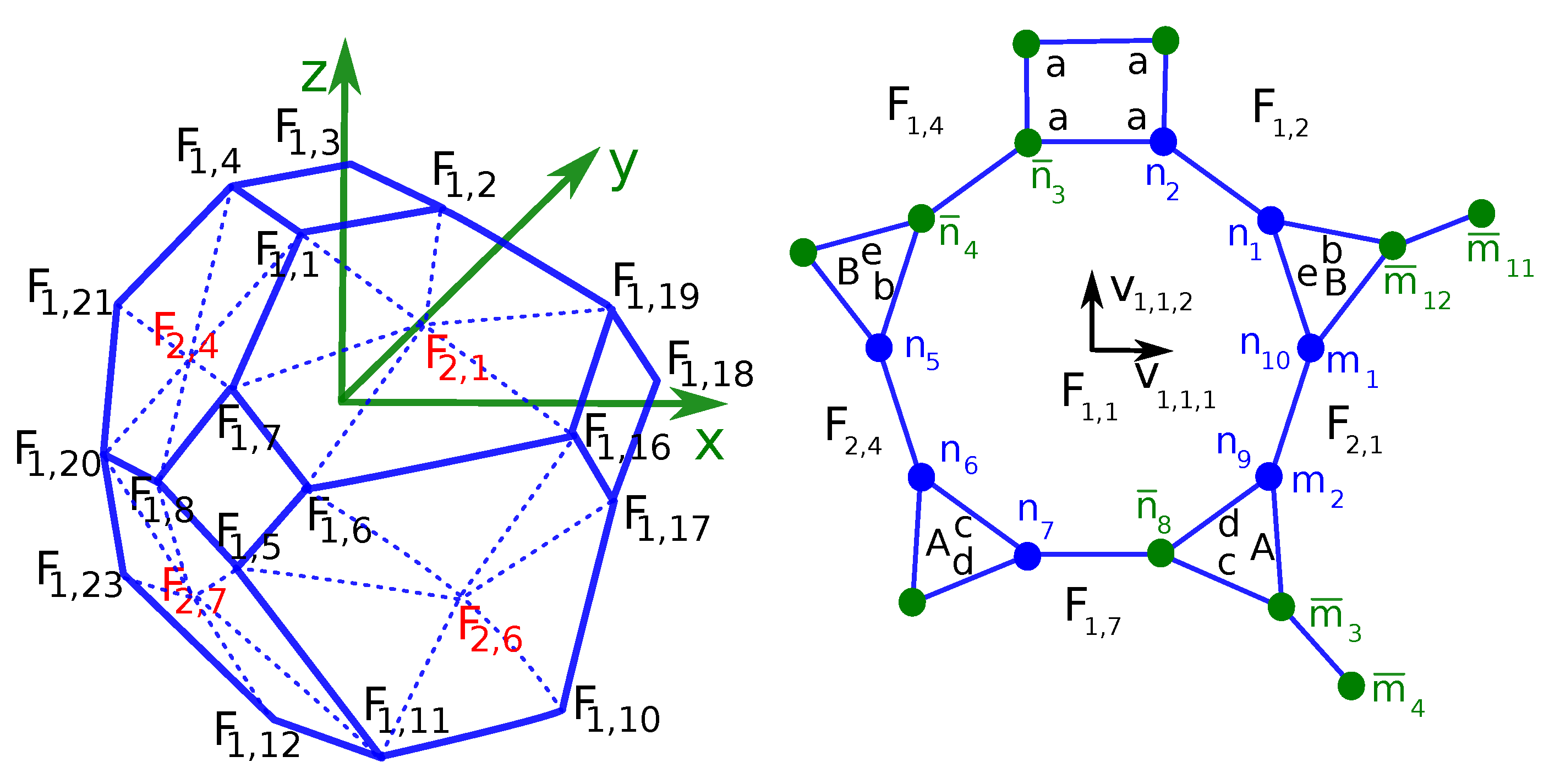
Figure 7.
Parametrisation of the pentakis dodecahedron PD p-cage. a) Pentakis dodecahedron vectors. b) Mapping of vertices.
Figure 7.
Parametrisation of the pentakis dodecahedron PD p-cage. a) Pentakis dodecahedron vectors. b) Mapping of vertices.
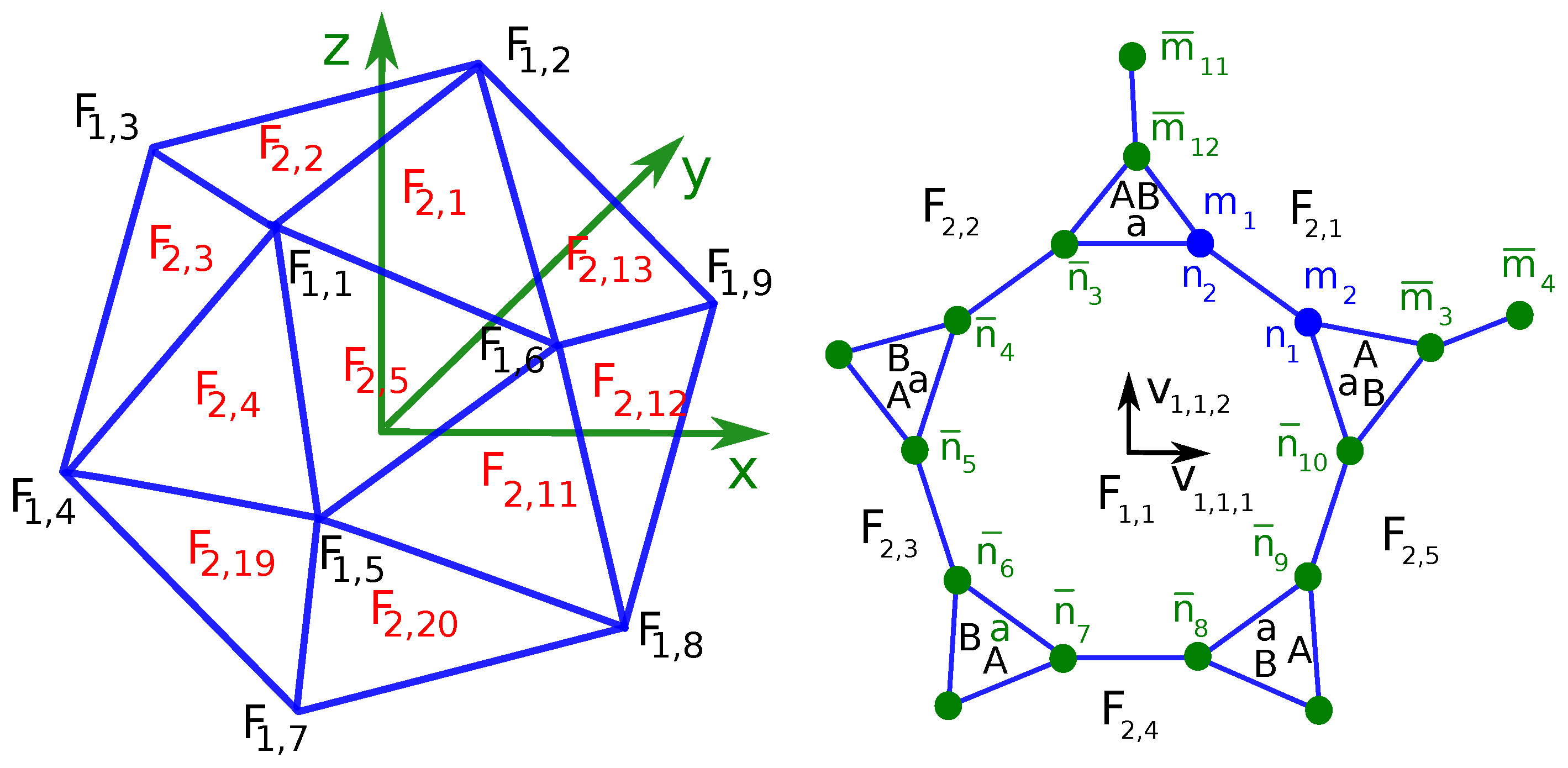
Figure 10.
Some of the least irregular p-cages: a) HAP6_P20_P24_5x3-6x3_cl0 , , b) PD_P20_P24_5x3-6x3, , c) PD_P15_P18_5x2-6x2, , d) PD_P10_P12_5x1-6x1, , e) IP5_P10_P12_5x1-6x1, , f) IP5_P10_P14_5x1-2_2x1_2_2x1, , g) TOP6_P11_P12_2_4x1-6x1, , h) TOP6_P16_P18_3_4x2-6x2, .
Figure 10.
Some of the least irregular p-cages: a) HAP6_P20_P24_5x3-6x3_cl0 , , b) PD_P20_P24_5x3-6x3, , c) PD_P15_P18_5x2-6x2, , d) PD_P10_P12_5x1-6x1, , e) IP5_P10_P12_5x1-6x1, , f) IP5_P10_P14_5x1-2_2x1_2_2x1, , g) TOP6_P11_P12_2_4x1-6x1, , h) TOP6_P16_P18_3_4x2-6x2, .
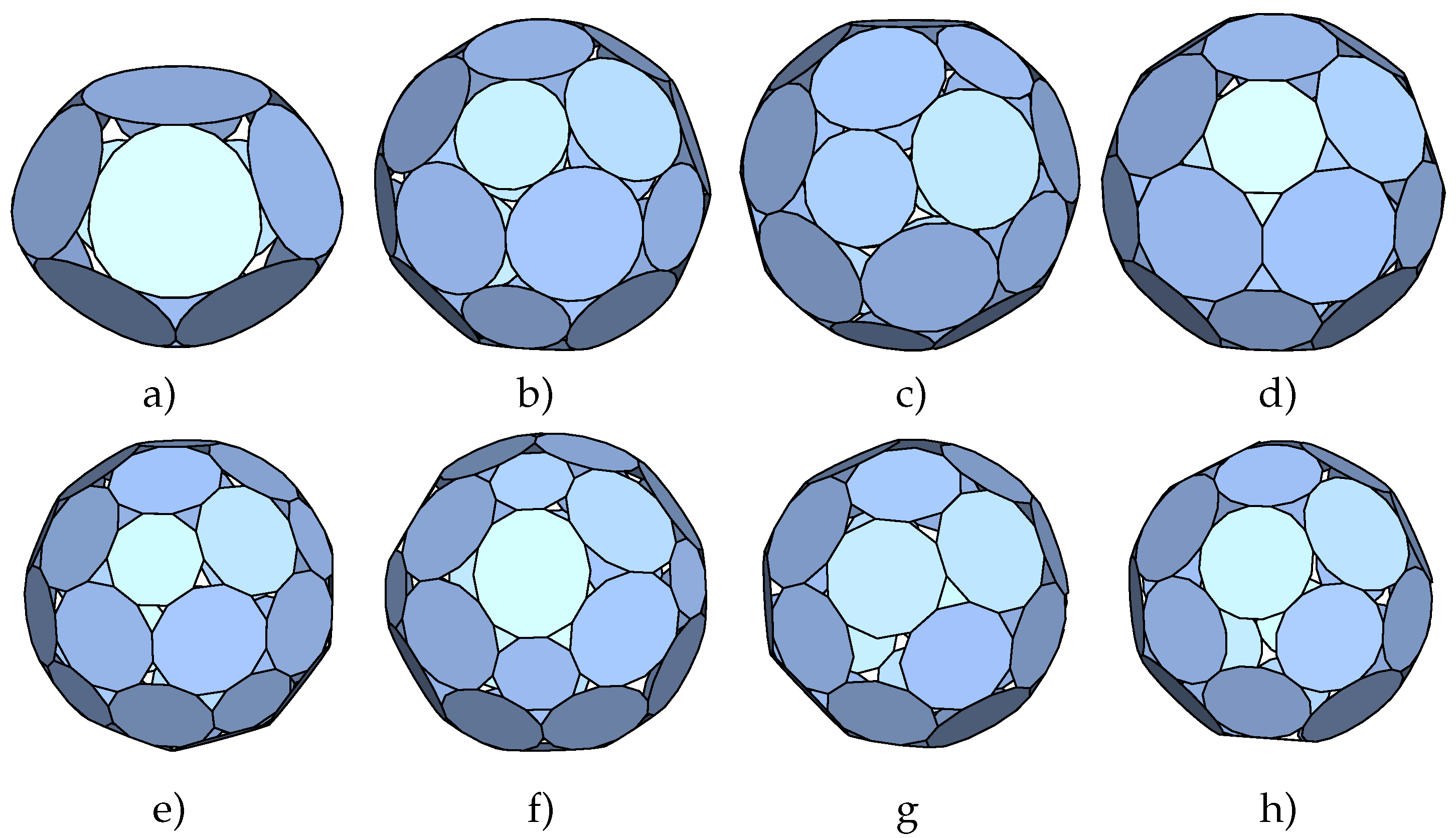
Figure 11.
Some of the least irregular p-cages: a) TTP6_P20_P24_5x3-6x3 , b) TTP6_P15_P18_5x2-6x2, c) TTP6_P10_P12_5x1-6x1, d) SDP5_P20_P24_5x3-6x3, e) SDP5_P15_P21_5x2-2x2_2x3_2_3, f) SDP5_P15_P18_5x2-6x2, g) SDP5_P10_P12_5x1-6x1, h) TCM4_P20_P24_5x3-6x3, .
Figure 11.
Some of the least irregular p-cages: a) TTP6_P20_P24_5x3-6x3 , b) TTP6_P15_P18_5x2-6x2, c) TTP6_P10_P12_5x1-6x1, d) SDP5_P20_P24_5x3-6x3, e) SDP5_P15_P21_5x2-2x2_2x3_2_3, f) SDP5_P15_P18_5x2-6x2, g) SDP5_P10_P12_5x1-6x1, h) TCM4_P20_P24_5x3-6x3, .
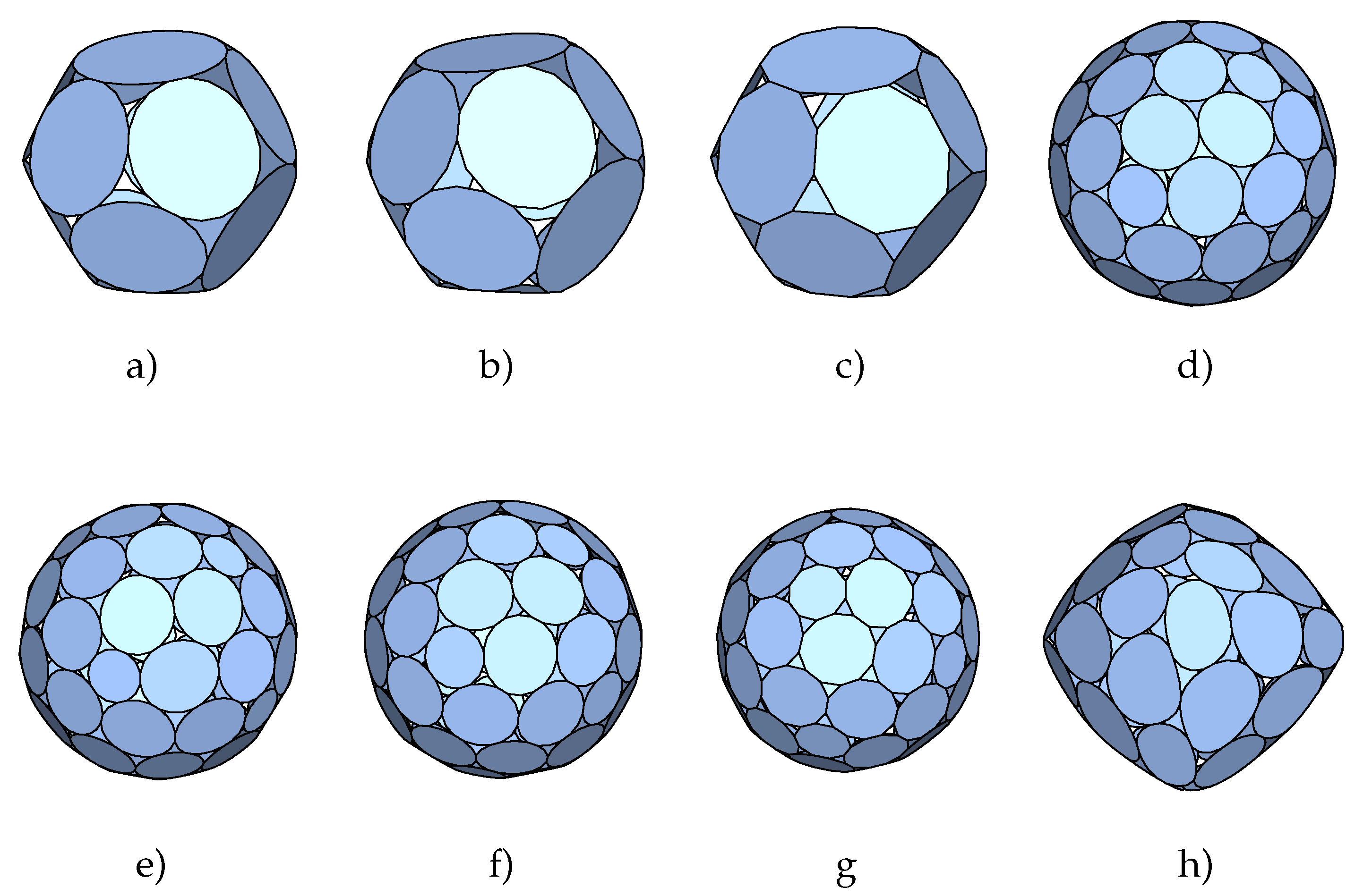

Table 1.
Bi-symmetric hole polyhedron graphs with valency 5 and 6 nodes as well as triangular and square faces [7]. The first column is the label we use to describe the p-cages derived from the graph, the second column is the label for the graph used in [7] and the third column describe a solid for which the planar graph corresponds to the hole polyhedron graph. N-mosaic were defined in [7] as 2N-gons with an extra edge attached to every other node.
| p-cage | graph name | Description |
|---|---|---|
| name | ||
| HAP6 | 56_F24_12-2-1_12-3-0_V12_2 | Hexagonal antiprism with a |
| hexagonal pyramid on each base | ||
| TTP6 | 56_F28_4-3-0_24-2-1_V12_4 | Truncated tetrahedron where a |
| pyramid is placed on each hexagons | ||
| TTM3 | 56_F44_4-0-3_4-3-0_12-2-1_24-1-2_V12_12 | Truncated tetrahedron where |
| the hexagons become 3-mosaic. | ||
| TOP6 | 56_F54_6-4-0_48-2-1_V24_8 | Truncated octahedron where a |
| pyramid is placed on the hexagons | ||
| PD | 56_F60_60-1-2_V12_20 | Pentakis dodecahedron |
| IP5 | 56_F80_20-0-3_60-1-2_V12_30 | Pyramids on the faces of an |
| icosidodecahedron. | ||
| TOM3 | 56_F86_6-0-4_8-3-0_24-2-1_48-1-2_V24_24 | Truncated octahedron where the |
| hexagons are 3-mosaic. | ||
| TCM4 | 56_F86_6-4-0_8-0-3_24-2-1_48-1-2_V24_24 | Truncated cube where the |
| octagons are 4-mosaic. | ||
| SDP5 | 56_F140_60-1-2_80-0-3_V12_60 | Pyramids on the faces of a snub |
| dodecahedron |
Disclaimer/Publisher’s Note: The statements, opinions and data contained in all publications are solely those of the individual author(s) and contributor(s) and not of MDPI and/or the editor(s). MDPI and/or the editor(s) disclaim responsibility for any injury to people or property resulting from any ideas, methods, instructions or products referred to in the content. |
© 2024 by the authors. Licensee MDPI, Basel, Switzerland. This article is an open access article distributed under the terms and conditions of the Creative Commons Attribution (CC BY) license (https://creativecommons.org/licenses/by/4.0/).
Copyright: This open access article is published under a Creative Commons CC BY 4.0 license, which permit the free download, distribution, and reuse, provided that the author and preprint are cited in any reuse.


