Submitted:
15 November 2024
Posted:
18 November 2024
You are already at the latest version
Abstract
Lung and bronchus cancer, collectively called lung cancer, remains one of the most lethal malignancies worldwide, with its incidence and mortality rates continuing to pose significant public health challenges. Numerous studies have explored various risk factors for lung cancer, including smoking, environmental pollutants, genetic predispositions, and occupational hazards. However, emerging research suggests that elevation above sea level may also influence lung and bronchus cancer prevalence and outcomes. We analyzed altitude data for 2,662 contiguous U.S. counties to determine if there is a significant relationship between lung cancer and elevation. Moreover, we employed hierarchical multiple regression and complex sample general linear model (CSGLM) to enhance understanding of the factors influencing lung and bronchus cancer, with a particular focus on elevation. Using the Local Moran’s I cluster analysis, we identified statistically significant hot spots and cold spots for the mortality rate related to lung cancer. In the hierarchical regression model, a significant correlation between lung cancer and elevation remained evident. This suggests that the risk of mortality from lung and bronchus cancer increases with decreasing elevation (R2 = 0.601). Furthermore, within the CSGLM framework, an R2 value of 0.763 highlighted a strong link between lung cancer mortality and elevation. This relationship remained significant even after accounting complex sample designs and applying weight adjustments. This geographic correlation has not been documented in previous studies. Further research is necessary to elucidate the precise mechanisms through which elevation influences lung cancer biology.
Keywords:
lung and bronchus cancer mortality rate
; elevation
; cluster analysis
; complex sample general linear model (CSGLM)
1. Introduction
Lung-bronchus cancer, collectively known as lung cancer, remains one of the most prevalent and deadly forms of cancer worldwide. According to the World Health Organization (WHO), lung cancer is the leading cause of cancer mortality, accounting for approximately 1.8 million deaths annually, which represents about 18% of all cancer deaths [1]. According to projections by the American Cancer Society, in 2023, the United States see approximately 238,340 new cases of lung and bronchus cancer, with an estimated 127,070 deaths resulting from the disease. Data from 2017–2019 indicates that about 6.1 percent of men and women will make a prognosis of lung and bronchus cancer in their lifetime [2,3]. The high mortality rate is primarily due to the disease's typically late diagnosis and its aggressive nature.
The major risk factor for lung cancer is tobacco smoking, responsible for about 85-90% of lung cancer cases. Other significant risk factors include exposure to radon gas, asbestos, and other carcinogens, as well as genetic predispositions and environmental pollutants [4]. Although lung cancer is closely linked to cigarette smoking, only approximately 15% of smokers develop the disease, and 10-15% of lung cancer cases occur in nonsmokers [5,6]. Such discrepancies in findings may be caused by various confounding factors and methodological challenges. For instance, differences in population genetics, lifestyle factors, smoking prevalence, healthcare access, and environmental exposures can all influence lung cancer risk and outcomes [7]. Moreover, the data quality and differences in study design can also impact the results and their interpretation.
Recent research indicates that environmental factors, including elevation above sea level, could significantly impact lung cancer incidence and outcomes. Studies exploring the link between elevation and lung cancer have provided supporting evidence, suggesting that higher altitudes, with their hypoxic conditions, might lower lung cancer incidence. The reduced oxygen levels found in high-altitude environments (hypoxia) can affect various biological processes in the human body, including those involved in cancer development and progression [8].
Nevertheless, the differences in lung cancer mortality rates across regions in the United States, along with the link between lung cancer and elevation, are still not fully understood. The relationship between geographic location and negative health outcomes is complex and multifaceted. Recent studies have begun to shed light on this prominent issue, investigating the disparities in various health outcomes, including lung cancer, across different geographic areas [9,10,11].
Moreover, in survey research, particularly when dealing with complex survey data, the application of statistical techniques such as stratification, clustering, and weighting is crucial for obtaining accurate, representative, and reliable results. These methods address the intricacies of survey designs and help mitigate biases, ensuring that the findings reflect the true characteristics of the population under study. Nevertheless, many researchers often handle these surveys as though they were unweighted simple random samples, which can lead to biased variance estimates and a higher risk of Type I errors [12,13,14]. In complex survey data, the combined use of stratification, clustering, and weighting addresses various challenges including improved precision and accuracy. These methods are indispensable techniques in the analysis of complex survey data. They ensure that survey estimates are precise, unbiased, and representative of the population, thereby enhancing the reliability and validity of the survey findings [12,13,14]. Software packages such as SPSS and Stata now feature modules that can adjust variance estimates for general linear models, logistic regressions, and ordinal regressions when dealing with complex sample designs [15,16].
Applying spatial regression in health studies is crucial for understanding and addressing geographic variations in health outcomes. Traditional regression models often fail to account for spatial dependencies, where health outcomes in one area may be influenced by those in neighboring regions. Spatial regression techniques correct for this spatial autocorrelation, leading to more accurate and unbiased estimates [17]. This is essential for identifying regional health disparities and environmental impacts on health, which can inform targeted public health interventions and resource allocation [18]. By incorporating spatial regression, health studies can better capture the complex spatial patterns inherent in health data, leading to improved understanding and more effective interventions [19].
2. Materials and Methods
2.1. Lung-Bronchus Cancer Mortality Data
This study examines the hypothesis that elevation significantly contributes to lung and bronchus cancer mortality by considering the impact of related risk factors. To test this hypothesis, data on age-adjusted lung and bronchus cancer mortality rates from 2016-2020 were gathered from State Cancer Profiles. Mortality data were sourced from the National Vital Statistics System public data file, and death rates were calculated by the National Cancer Institute using SEER Stat. These death rates (deaths per 100,000 population per year) are adjusted to the 2010 US Standard population. Figure 1 presents lung and bronchus cancer mortality rates across 2,662 contiguous counties from 2016 to 2020.
2.2. Mean County Elevation Data
County elevation data for 3,141 administrative areas within the U.S. was created by the U.S. Geological Survey [20]. The mean altitude for each county was accurately calculated using the 100-meter spatial resolution of the USGS dataset. Zonal statistics within the ArcGIS 10.5 were utilized to compute the mean altitude for each county, minimizing variations in topography. This method is more reliable, even for large counties, although challenges are more pronounced when considering entire states [21] or using elevation values from the county centers [22]. The analysis included data from 3,064 contiguous counties. County boundaries from the U.S. Census Bureau were used to obtain the mean county altitudes in meters and the area in square miles for each county, as illustrated in Figure 2.
2.3. Potential Confounders
To improve the reliability of our analyses, we accounted for several confounding factors as detailed by Tu et al. (2020) [23]. These include: (1) health behavior factors like the percentage of adult smokers, insufficient sleep, adult obesity, the food environment index, physical inactivity, and alcohol impairment; (2) clinical care factors, such as the proportion of uninsured individuals, the ratio of primary care physicians to the population, and rates of preventable hospitalizations; (3) social and economic factors, including the percentage of the population with a college education, unemployment rates, household income at the 80th percentile, and the number of membership associations per 10,000 people; (4) physical environmental factors, such as the average daily PM2.5 concentration; and (5) demographic factors, including the percentage of individuals aged 65 and older, the proportion of African American residents, the percentage of female residents, and the proportion of the population living in rural areas. Due to the limited availability of variables related to mental health conditions in the SMART BRFSS, we had to source data on potential confounding factors from various other datasets [24].
For health behaviors, such as the percentage of adult smokers and obesity rates, data were obtained from both the BRFSS and the CDC Diabetes Interactive Atlas. Clinical care information, including the ratio of uninsured adults and the ratio of primary care physicians, was retrieved from the Small Area Health Insurance Estimates (SAHIE) and the American Medical Association (AMA). Data on preventable hospital stays were sourced from the Dartmouth Atlas of Health Care. Additionally, information on the percentage of individuals holding a college degree was gathered from the American Community Survey (ACS), while data on social associations came from the County Business Patterns. Lastly, demographic factors such as the percentage of adults aged 65 and older, the percentage of African Americans, the percentage of females, and the percentage of rural residents were all obtained from Census Population Estimates [24].
2.4. Model Analysis
This study was conducted in three steps to examine the variations in the relationship between lung-bronchus cancer mortality rates and elevation over different geographic areas. In the initial stage, we evaluated skewness before data analysis to ascertain if any variables needed transformation, concluding that no transformation was required. In the second stage, we integrated elevation with potential confounding factors on the lung-bronchus cancer into a stepwise regression model. Our primary objective was to investigate the relationship between lung-bronchus cancer mortality rates and insufficient sleep, so we employed a hierarchical multiple regression model. Firstly, the model included only the elevation. In the next step, we added potential confounding factors in a second regression model to ensure that their inclusion did not alter the significance of elevation in affecting the lung-bronchus cancer mortality rate. In the final stage, it is critical to analyze all BRFSS data, including SMART data, using statistical methods that account for the complex sampling design and weighting adjustments. This step is vital to avoid incorrect variance estimates and to reduce the likelihood of Type I errors (false positives) [15,16]. To accomplish this, we utilized the Complex Samples General Linear Model (CSGLM) in SPSS. This approach adjusts variance estimates for GLM within complex sample designs [10].
2.5. Local Mortan’s I Analysis
Local Moran's I is a powerful tool used in spatial statistics to identify clusters or outliers of spatial data. Unlike the global Moran's I, which provides a single measure of spatial autocorrelation for an entire dataset, Local Moran's I focuses on individual locations, revealing the local patterns of spatial association. This local indicator of spatial association (LISA) is instrumental in pinpointing specific areas of high or low values that deviate significantly from the overall spatial pattern [25].
The formula for Local Moran's I for a specific location i is given by:
where:
- zi is the deviation of the value at location i from the mean,
- wi,j is the spatial weight between location i and location j,
- xj and xj are the values of the variable of interest at locations i and j, respectively,
- x̄ is the mean of the variable across all locations,
- n is the total number of locations.
The Local Moran's I helps in identifying local clusters (high-high or low-low) and spatial outliers (high-low or low-high). A high positive value of Ii indicates that location i is surrounded by locations with similar high or low values (cluster), while a negative value suggests a spatial outlier, where location i is surrounded by locations with dissimilar values [25]. Spatial analysis software, such as ArcGIS, GeoDa, and R, provides tools for computing Local Moran's I and visualizing the results through cluster maps. These visualizations are crucial for interpreting the spatial patterns and making informed decisions based on the analysis [26].
3. Results
3.1. Descriptive Statistics
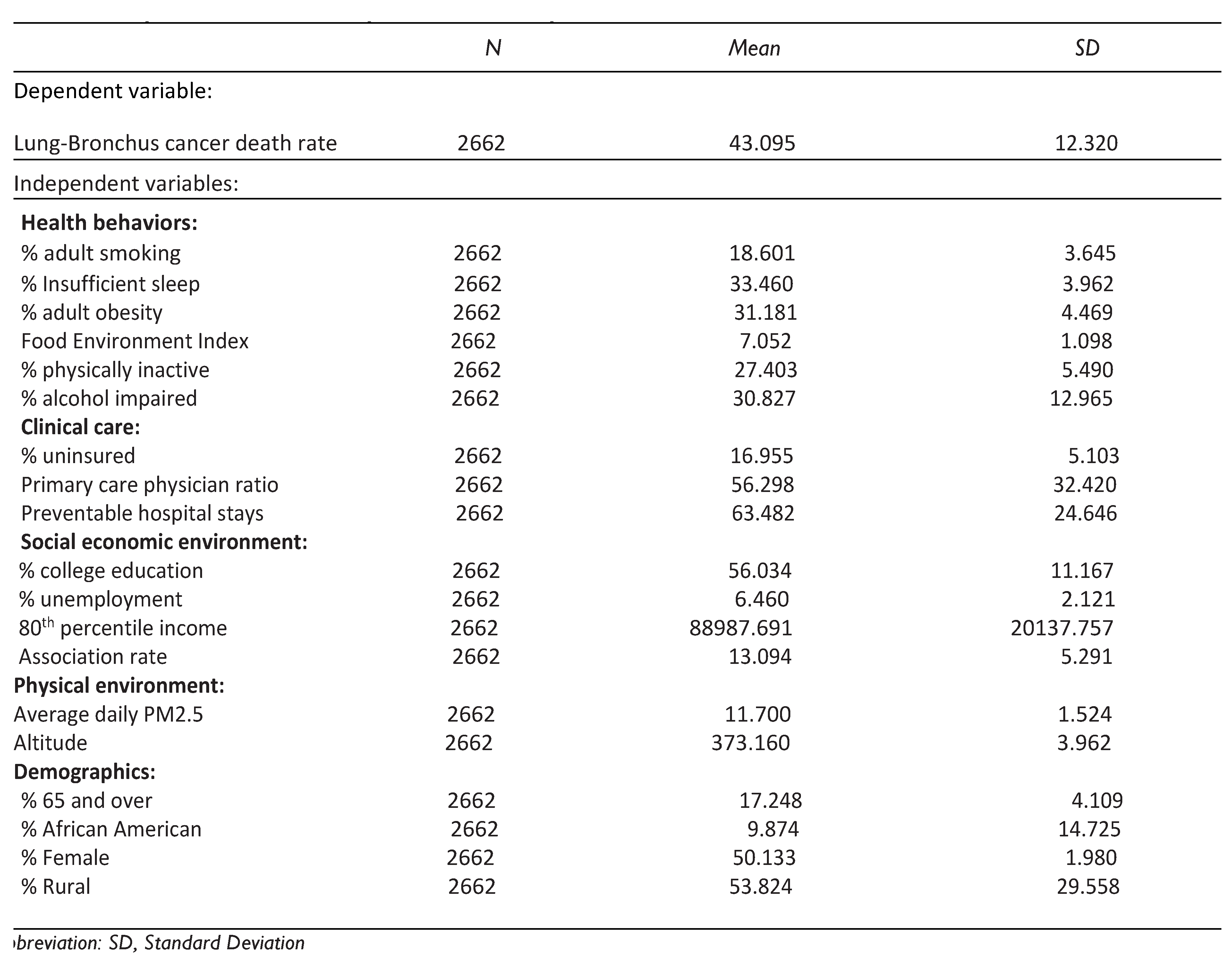
Table 1 provides a summary of the statistics for all the variables used in this study. These statistics indicate that the values of these variables differ significantly among counties within the state. The research included 2,662 contiguous counties in the United States. The exploratory variables showed variation across these counties, suggesting that areas with differing health behaviours, clinical practices, socioeconomic status, and demographic traits experienced different rates of lung-bronchus cancer mortality.
3.2. Hierarchical Regression Analyses
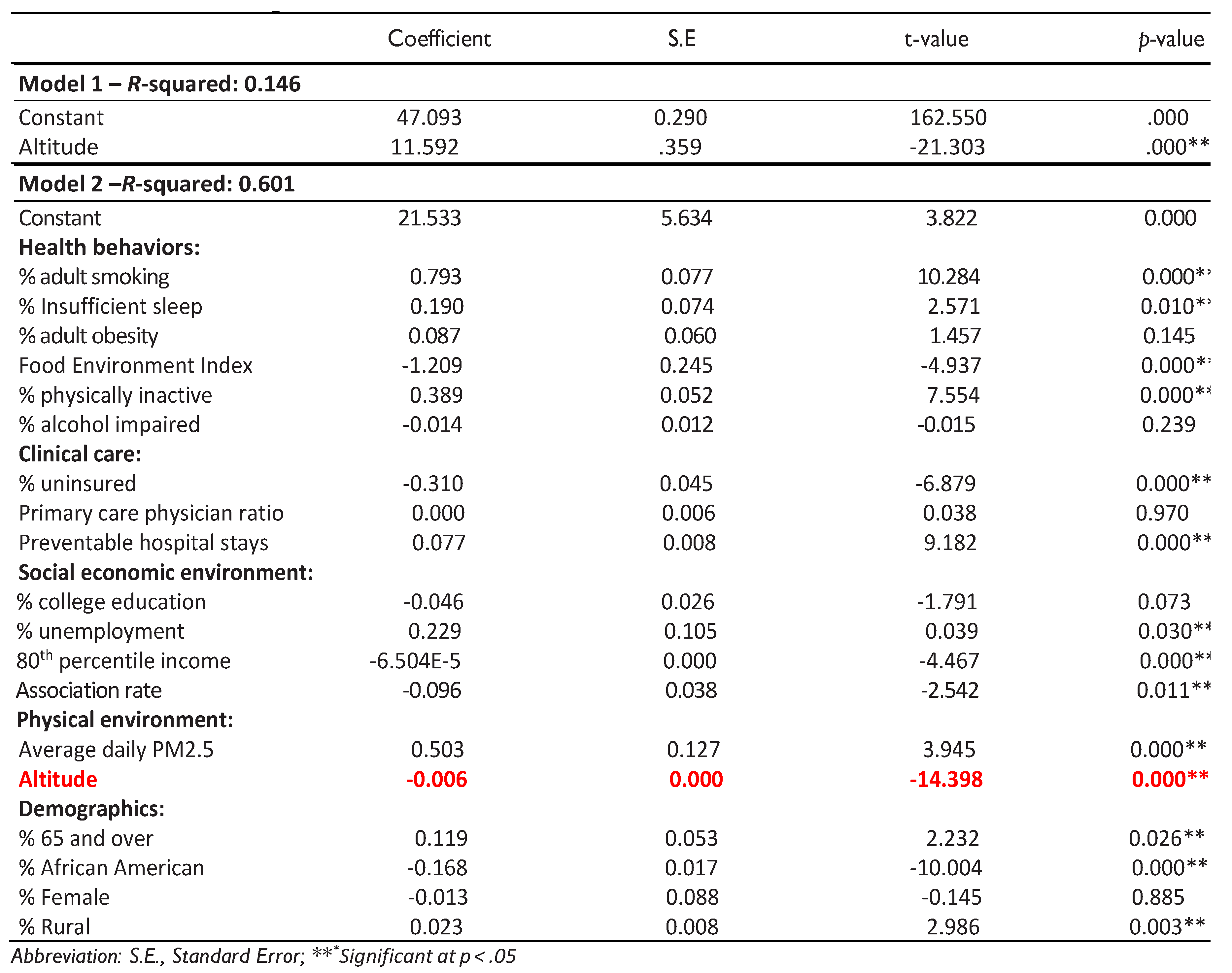
Model 1 demonstrated that the regression model only with the elevation factor was statistically significant, as indicated by an F-value of (1, 2660) = 453.826 and a p-value of less than 0.001. This model accounted for approximately 14.6% of the variance in lung-bronchus cancer mortality rates. As shown in Table 2, there was a significant relationship between elevation and lung-bronchus cancer mortality rate (β = -0.011; p = 0.000). Despite including only elevation, one independent variable, the regression model's R² value of 0.146 explained a significant portion of the variability in lung-bronchus cancer mortality rates across the numerous counties studied.
In Model 2, the subsequent hierarchical regression analysis included 19 variables and revealed that the overall model was statistically significant, with an F-value of (19, 2642) = 209.227 and a p-value of less than 0.001. This model explained 60.1% of the variability in lung-bronchus cancer mortality rates. The regression analysis indicated that several variables were significantly associated with lung-bronchus cancer mortality rates, including elevation, percent of adult smokers, percent of insufficient sleep, food environment index, physical inactivity rate, percent of uninsured individuals, preventable hospital stays, percent of unemployment, 80th percentile income, association rate, average daily density of PM2.5, percent of 65 and older, percent of African American individuals, and percent of rural residents, as illustrated in Table 2.
The results indicate that as the percentage of people residing at high elevation increases, the rate of mortality from lung-bronchus cancer decreases. Even after controlling for other potential confounding factors that might influence this relationship, elevation remained a significant predictor of lung-bronchus cancer mortality rates.

Table 2.
Hierarchical regression models.
 |
3.3. CSGLM Analyses
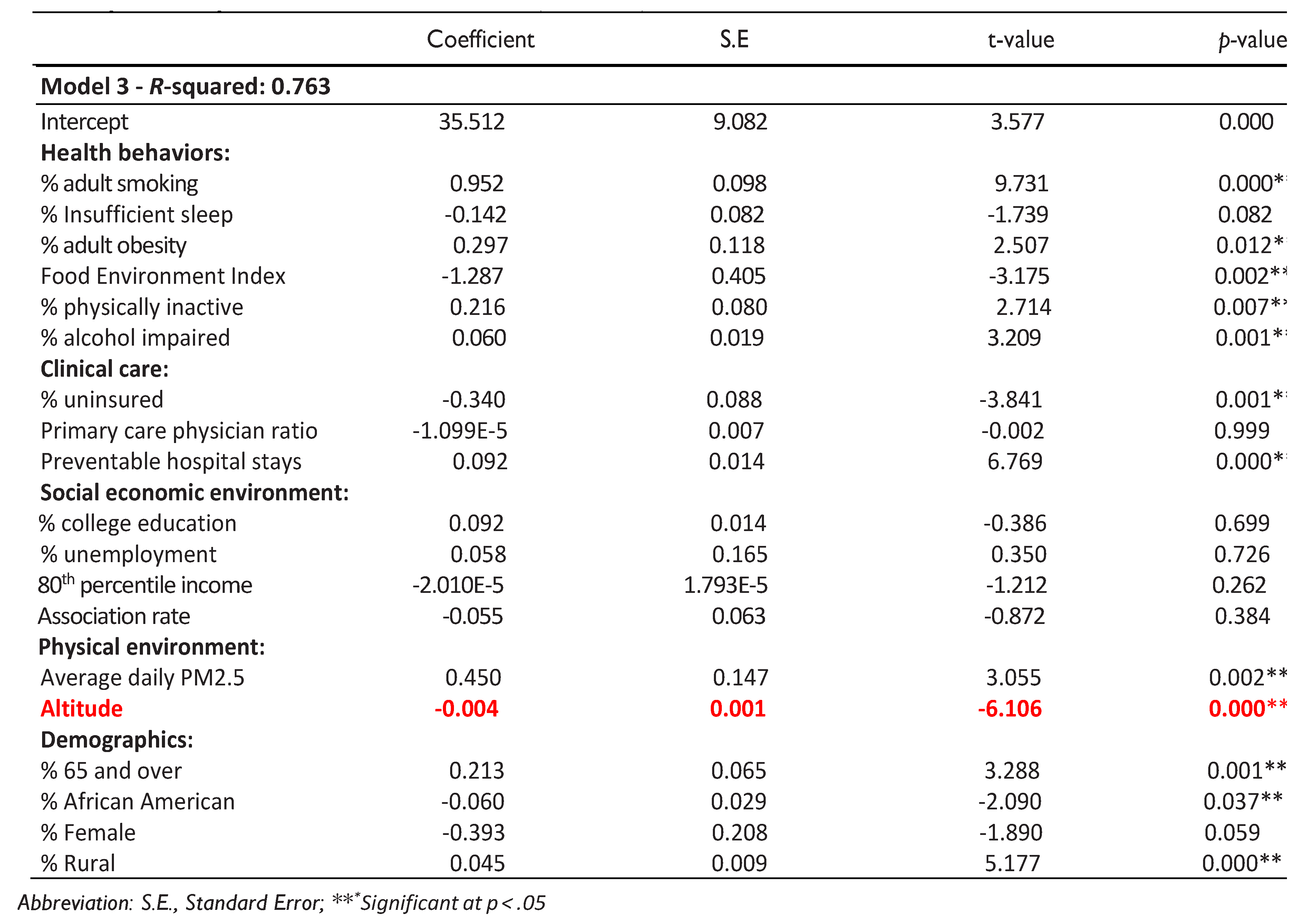
The Complex Samples General Linear Model (CSGLM) technique is used to build on previous quantitative research exploring the link between lung-bronchus cancer mortality rates and elevation. This method considers complex sampling designs and adjusts for weights to provide accurate estimates of the key factors influencing lung-bronchus cancer mortality rates [10,24]. Model 3 in Table 3 shows the results of the CSGLM regression, indicating that the model explains approximately 80% of the variation in lung-bronchus cancer mortality rates at the county level, as evidenced by an R-squared value of 76.3%. Out of the 19 independent variables analyzed, 12 were found to be significantly associated with lung-bronchus cancer mortality rates, with p-values below 0.05.
The study’s findings indicate that lung-bronchus cancer mortality rates vary greatly across different counties and are impacted by numerous factors, such as health behaviors, clinical care, socioeconomic conditions, physical environment, and demographic factors. The percent of adult smokers, adult obesity rates, food environmental index, physical inactivity rate, and percent of alcohol impairment are all health behavior variables that have a strong positive correlation with lung-bronchus cancer mortality. In terms of clinical care, there is a significant negative association between the ratio of uninsured individuals and the mortality rate from lung-bronchus cancer. Moreover, physical environmental factor, particularly elevation, is inversely related to lung-bronchus cancer mortality rates, suggesting that higher elevation is associated with reduced mortality. In contrast, for another physical environmental factor, averaged daily PM2.5 is positively associated with the cancer mortality rate. Finally, among the demographic variables, the percentage of the population aged 65 and older and the proportion of rural residents have a positive correlation with lung-bronchus cancer mortality, whereas the percentage of African American has a negative correlation with mortality rates. Overall, the CSGLM study’s results demonstrate that lung-bronchus cancer prevalence varies significantly across counties, influenced by a complex array of factors, including elevation.
Table 3.
Hierarchical regression models.
 |
3.4. Local Moran’s I Analyses
Figure 3 illustrates the spatial distribution of local Moran’s I for lung-bronchus cancer mortality rates across the 48 contiguous states in the U.S. The high-high clusters, which represent areas with higher lung-bronchus cancer mortality, are mainly concentrated in the southeastern and central regions, including states like Alabama, Arkansas, Georgia, Kentucky, Louisiana, Mississippi, Missouri, Oklahoma, and Tennessee. These areas also report relatively lower levels of elevation. In contrast, the low-low clusters, or areas with lower lung-bronchus cancer mortality rates, are largely located in the Western and Midwestern parts of the country, especially in states such as Arizona, Colorado, Idaho, New Mexico, Utah, and Wyoming, where are placed relatively higher elevation. Additionally, the global Moran’s I test shows a value of 0.469 with a z-score of 109.355 and a p-value of less than 0.001, confirming that there is a statistically significant spatial clustering of lung-bronchus cancer death rates at the county level across the United States.
4. Discussion
Altitude has been shown to have an inverse relationship with lung-bronchus cancer mortality rates, where higher elevations are associated with lower death rates from this cancer type. One possible explanation for this phenomenon is the reduced oxygen levels at higher altitudes, which may lead to lower atmospheric pressure and a decrease in the proliferation of cancer cells. Hypoxia, a condition that occurs when the body or a region of the body is deprived of adequate oxygen supply, can inhibit the growth of tumors due to reduced oxygen levels essential for cancer cell survival and growth. This idea is supported by studies that suggest that living at higher altitudes may expose individuals to chronic hypoxia, which could suppress tumor growth and reduce cancer incidence and mortality [27,28].
However, it is essential to consider that while altitude may play an important role in reducing lung-bronchus cancer mortality rates, this relationship is likely influenced by a complex interplay of other factors such as socioeconomic status, access to healthcare, and regional health behaviors. For instance, higher altitudes are often associated with rural settings, where population density is lower, and lifestyle factors such as reduced exposure to pollution or smoking may also contribute to lower cancer rates. Additionally, the physical environment, including cleaner air and lower levels of industrial pollutants at higher altitudes, might further influence these mortality rates [27,29]. After adjusting for these confounding factors, it was found that counties with a higher altitude showed relatively lower lung-bronchus cancer mortality rates. This study is the first to explore the connection between altitude and the variation in lung-bronchus cancer death rates across different geographic regions. The results indicate a need for further research to comprehensively understand the role of altitude in decreasing lung-bronchus cancer death rates.
The study identified the southeastern and central United States, including states such as Alabama, Arkansas, Georgia, Kentucky, Louisiana, Mississippi, Missouri, Oklahoma, and Tennessee, as a region with the highest concentration of high lung-bronchus cancer death rates. Conversely, regions with lower rates of lung-bronchus death rates, referred to as cold spots, are primarily located in the Midwest and Western U.S including Arizona, Colorado, Idaho, New Mexico, Utah, and Wyoming. Prior research consistently highlights that the southeastern region of the United States, also referred to as the "Stroke Belt" or the "Diabetes Belt" is identified as the least healthy region in the country, with its residents experiencing higher risks of various chronic diseases. such as obesity [30,31], cardiovascular disease [30,32], and diabetes [33]. The poor health outcomes in the southeastern United States may be linked to unhealthy behaviors, socioeconomic challenges, limited access to healthcare, and higher premature mortality [34,35].
Furthermore, this research builds upon previous studies examining the link between altitude and lung-bronchus cancer death rates. It demonstrates that using the Complex Samples General Linear Model (CSGLM) offers a more accurate representation of the data compared to the Ordinary Least Squares (OLS) method, as it considers complex sample designs and incorporates stratification, clustering, and weight adjustments. The R² value obtained from the CSGLM model is higher than the OLS model's R² value of 0.601. This increase may be attributed to the fact that CSGLM corrects for the biases introduced by complex design factors, providing more accurate parameter estimates of the significant variables influencing lung-bronchus cancer death rates [10].
This study's approach to exploring the connection between altitude and lung-bronchus cancer death rates has some limitations. First, the analysis relied on aggregated data at the county level, which does not capture variations in altitude and lung-bronchus cancer death rates within individual counties. This could result in ecological fallacies, where incorrect assumptions about individuals are made based on group-level data. To strengthen the validity of these findings, future research should utilize individual-level data or data from countries outside the United States [10,24]. Additionally, another limitation lies in the sensitivity or uncertainty of hotspot analysis, especially regarding how spatial relationships are defined and measured.
5. Conclusions
This study revealed that the association between altitude and lung-bronchus cancer mortality rates varies across different regions in the United States. Our analysis demonstrated that altitude is significantly related to lung-bronchus cancer death rates in U.S. counties, even after controlling for 18 confounding variables. These variables include (1) health behaviors such as percent of adult smokers, percent of insufficient sleep, percent of adult obesity, food environment index, percent of adults who are physically inactive, and percent of alcohol-impairment; (2) clinical care variables including percent of uninsured individuals, ratio of primary care physicians to the population, and preventable hospital stays; (3) social and economic variables such as percent of population with a college degree, percent of unemployment, ratio of household of income at the 80th percentile, and number of membership associations per 10,000; (4) physical environmental variable includes average daily density of PM2.5 and (5) demographic variables, including percent of 65 and older, percent of African American individuals, percent of females, and percent of rural residents.
The findings indicate that addressing altitude could be a protective strategy for reducing lung-bronchus cancer death rates. However, it is also clear that lung-bronchus cancer is significantly associated with other confounding variables including the percent of adult smokers and preventable hospital stays. While this study highlights the influence of altitude on lung-bronchus cancer, it is not the sole contributing factor. Health policies must consider the role of altitude alongside other social and environmental variables in different communities to more effectively address lung-bronchus cancer mortality. Future research should aim to identify and understand the complex mechanisms through which altitude influences lung-bronchus cancer.
Author Contributions
Hoehun Ha performed the data curation, statistical analyses and wrote the manuscript.
Funding
This research did not receive any specific grant from funding agencies in the public, commercial, or not-for-profit sectors.
Data Availability Statement
Data are contained within this article.
Acknowledgments
The author would like to thank the anonymous reviewers for their constructive comments and suggestions to improve the paper. The contents of this publication are solely the responsibility of the authors.
Conflicts of Interest
The authors declare no conflict of interest.
References
- WHO. (2021). Cancer. Retrieved from https://www.who.int/news-room/fact-sheets/detail/cancer.
- American Cancer Society (2023). Cancer Facts and Figures 2023. Atlanta; American Cancer Society.
- NIH (2023). Cancer Stat Facts: Lung and Bronchus Cancer. Retrieved June 11, 2023, from https://seer.cancer.gov/statfacts/html/lungb.html.
- American Cancer Society. (2021). Lung Cancer Risk Factors. Retrieved June 11, 2023, from https://www.cancer.org/cancer/lung-cancer/causes-risks-prevention/risk-factors.html.
- Samet JM, Avila-Tang E, Boffetta P, Hannan LM, Olivo-Marston S, Thun MJ, Rudin CM. (2009). Lung cancer in never smokers: clinical epidemiology and environmental risk factors. Clinical Cancer Research 15(18):5626–5645 . [CrossRef]
- Kuśnierczyk, P. (2023). Genetic differences between smokers and never-smokers with lung cancer. Front Immunology, 14. [CrossRef]
- Zhu, X., Lu, Y., Shen, T., & Dong, W. (2019). Socioeconomic status and lung cancer risk: A meta-analysis. Translational Lung Cancer Research, 8(4), 412-428.
- Ward, M. P., Milledge, J. S., & West, J. B. (2000). High Altitude Medicine and Physiology. CRC Press.
- Baciu, A., Negussie, Y., & Geller, A. (2017). The state of health disparities in the United States. Washington (DC): National Academies Press (US).
- Ha, H. (2023). Spatial variations in the associations of mental distress with sleep insufficiency in the United States: a county-level spatial analysis. International Journal of Environmental Health Research. [CrossRef]
- Ha, H., & Tu, W. (2018). An ecological study on the spatially varying relationship between county-level suicide rates and altitude in the United States. International Journal of Environmental Research and Public Health, 15(4):671. [CrossRef]
- Bethlehem, J. (2009). Applied Survey Methods: A Statistical Perspective. Wiley.
- Heeringa, S. G., West, B. T., & Berglund, P. A. (2017). Applied Survey Data Analysis. Chapman and Hall/CRC.
- Lohr, S. L. (2019). Sampling: Design and Analysis. Chapman and Hall/CRC.
- Campbell, R.T., & Berbaum, M.L. (2010). Analysis of data from complex survey in a handbook of survey research (editor Marsden P.V). Emerald, pp 221-262.
- Sturgis, P. (2004). Analyzing complex survey data: clustering, stratification and weights. Soc res update. 43Autumn issue. Surrey: University of Surrey.
- Anselin, L. (1988). Spatial Econometrics: Methods and Models. Kluwer Academic Publishers.
- Cromley, E. K., & McLafferty, S. L. (2011). GIS and Public Health. Guilford Press.
- Pfeiffer, D. U., Robinson, T. P., Stevenson, M., Stevens, K. B., Rogers, D. J., & Clements, A. C. A. (2008). Spatial Analysis in Epidemiology. Oxford University Press.
- U.S. Geological Survey. (2012). 100-Meter Resolution Elevation of the Conterminous United States. https://catalog.data.gov/dataset/100-meter-resolution-elevation-of-the-conterminous-united-states-direct-download.
- Huber, R.S, Kim, T, Kim, N, Kuykendall, M.D, Sherwood, S.N, Renshaw, P.F, and Kondo, D.G. (2015). Association between altitude and regional variation of ADHD in youth. Journal of Attention Disorders. [CrossRef]
- Brenner B, Cheng D, Clark S, and Camargo CA Jr. (2011). Positive association between altitude and suicide in 2584 U.S. counties. High Alt Med Bio 12: 31-35. [CrossRef]
- Tu, W., Ha, H., Wang, W., & Liu, L. (2020). Investigating the association between household firearm ownership and suicide rates in the United States using spatial regression models. Applied Geography, 124. [CrossRef]
- Ha, H. (2018). Using geographically weighted regression for social inequality analysis: association between mentally unhealthy days (MUDs) and socioeconomic status (SES) in U.S. counties. International Journal of Environmental Health Research, 29(2):140–153. [CrossRef]
- Anselin, L. (1995). Local Indicators of Spatial Association—LISA. Geographical Analysis, 27(2), 93-115. [CrossRef]
- Ord, J. K., & Getis, A. (1995). Local Spatial Autocorrelation Statistics: Distributional Issues and an Application. Geographical Analysis, 27(4), 286-306.
- Burtscher, J., Mallet, R. T., Burtscher, M., & Millet, G. P. (2021). Hypoxia and brain aging: Neurodegeneration or neuroprotection? Ageing Research Reviews, 68, 101343. [CrossRef]
- Moore, L. G., Niermeyer, S., & Zamudio, S. (1998). Human adaptation to high altitude: Regional and life-cycle perspectives. American Journal of Biological Anthropology, 41, 25-64. [CrossRef]
- West, J. B. (2016). High-altitude medicine and physiology. CRC Press.
- Akil, L., & Ahmad, H.A. (2011). Relationships between Obesity and Cardiovascular Diseases in Four Southern States and Colorado. Journal of Health Care for the Poor and Underserved, 22(4): 61-72. [CrossRef]
- CDC. (2024). Adult Obesity Prevalence Maps. https://www.cdc.gov/obesity/php/data-research/adult-obesity-prevalence-maps.html. Accessed 20 August 2024.
- Casper, M. L., Barnett, E., Williams, G. I., Halverson, J. A., Braham, V. E., & Greenlund, K. J. (2003). Atlas of stroke mortality: Racial, ethnic, and geographic disparities in the United States. Centers for Disease Control and Prevention.
- Barker, L. E., Kirtland, K. A., Gregg, E. W., Geiss, L. S., & Thompson, T. J. (2011). Geographic distribution of diagnosed diabetes in the U.S.: A diabetes belt. American Journal of Preventive Medicine, 40(4), 434-439. [CrossRef]
- Adler, N. E., & Newman, K. (2002). Socioeconomic disparities in health: Pathways and policies. Health Affairs, 21(2), 60-76. [CrossRef]
- Williams, D. R., & Jackson, P. B. (2005). Social sources of racial disparities in health. Health Affairs, 24(2), 325-334. [CrossRef]
Figure 1.
County-level lung-bronchus cancer death rate across 3,064 contiguous U.S. counties.
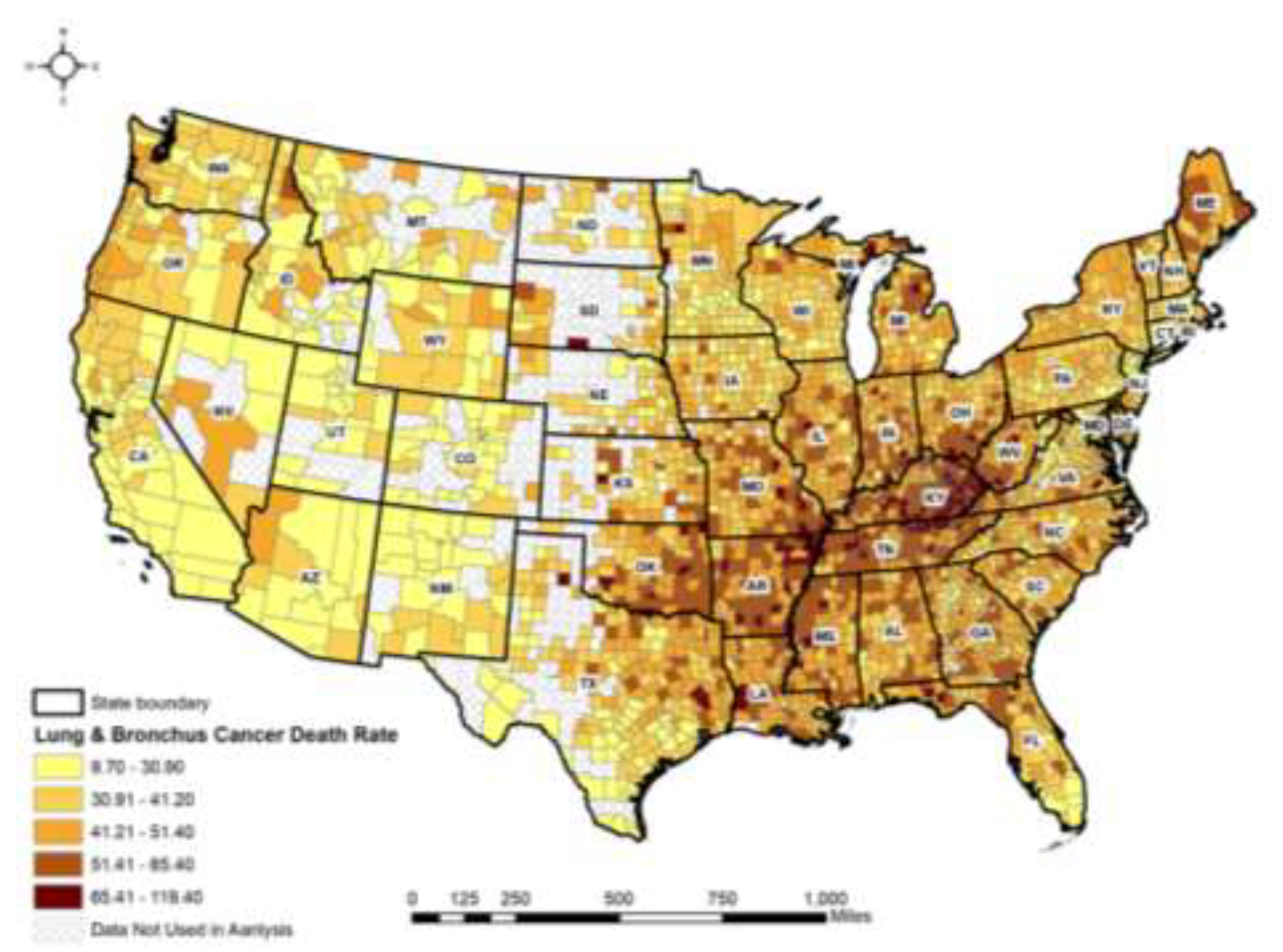
Figure 2.
Mean county elevation across 3,064 contiguous U.S. counties.
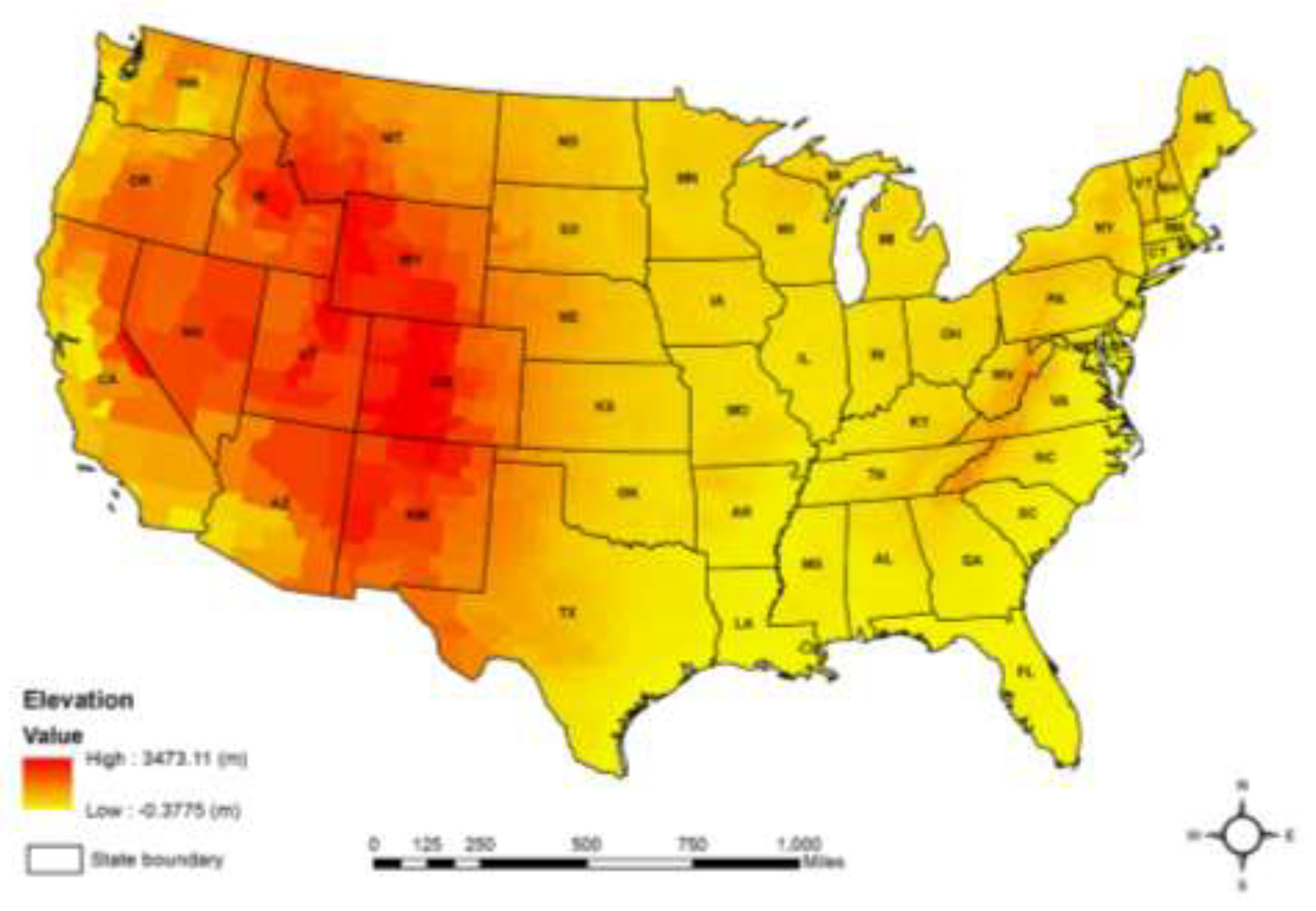
Figure 3.
County-level local Moran’s I of lung-bronchus cancer death rate in the contiguous US states.
Figure 3.
County-level local Moran’s I of lung-bronchus cancer death rate in the contiguous US states.
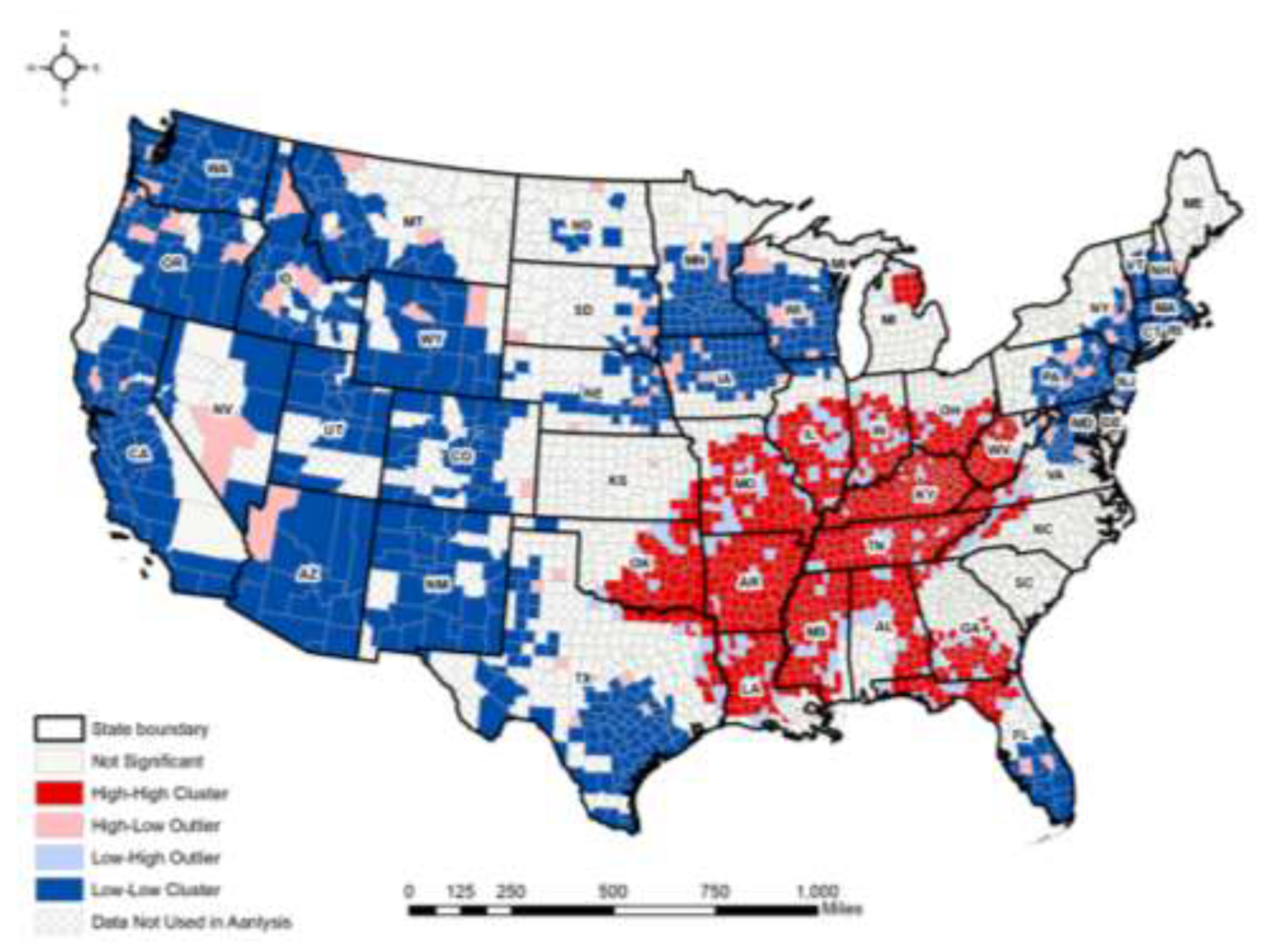
Table 1.
Descriptive statistics for dependent and independent variables.
 |
Disclaimer/Publisher’s Note: The statements, opinions and data contained in all publications are solely those of the individual author(s) and contributor(s) and not of MDPI and/or the editor(s). MDPI and/or the editor(s) disclaim responsibility for any injury to people or property resulting from any ideas, methods, instructions or products referred to in the content. |
© 2024 by the authors. Licensee MDPI, Basel, Switzerland. This article is an open access article distributed under the terms and conditions of the Creative Commons Attribution (CC BY) license (http://creativecommons.org/licenses/by/4.0/).
Copyright: This open access article is published under a Creative Commons CC BY 4.0 license, which permit the free download, distribution, and reuse, provided that the author and preprint are cited in any reuse.


