Deep Learning-Based Algorithms for Real-Time Lung Ultrasound Assisted Diagnosis

Lung ultrasound is an increasingly utilized non-invasive imaging modality for assessing the lung condition, but interpreting it can be challenging and depends on the operator experience. To address these challenges, this work proposes an approach that combines artificial intelligence (AI) with feature-based signal processing algorithms. We introduce a specialized deep learning model designed and trained to facilitate the analysis and interpretation of lung ultrasound images, by automating the detection and location of pulmonary features, including the pleura, A-lines, B-lines and consolidations. Employing Convolutional Neural Networks (CNNs) trained on a semi-automatically annotated dataset, the model delineates these pulmonary patterns, with the objective of enhancing diagnostic precision. Real-time post-processing algorithms further refine prediction accuracy by reducing false-positives and false-negatives, augmenting interpretational clarity and obtaining a final processing rate of up to 20 frames per second withl accuracies of 89% for consolidation, 92% for B-lines and 66% in case of A-lines compared with an expert opinion.

Keywords:

Lung ultrasound (LUS)

;

Artificial Intelligence (AI)

;

Convolutional Neural Network

;

Deep Learning

;

pleura

;

B-line

;

A-line

;

consolidations

;

assisted diagnosis

;

real-time

Subject:

Engineering - Bioengineering

1. Introduction

Within the field of diagnostic imaging, lung ultrasound (LUS) has become significantly more prominent in the last years, offering a non-invasive, radiation-free approach for dynamic assessment of lung condition in various respiratory diseases [1]. Yet, despite its growing importance, the interpretation challenges inherent to pulmonary ultrasound images persist, which combined with a shortage of skilled professionals trained in this technique, limits its application in clinical practice [2].

LUS images do not provide an anatomical view of the lung, because ultrasound waves hardly penetrate into the lung parenchyma because of the air presence in the alveoli. Instead, most of the acoustic energy is reflected by the pleura, which is the most easily identifiable structure, appearing like a bright horizontal line. Furthermore, replicas of the pleura appear at regular intervals below this line, generated by the reverberation of the incident wave between the transducer and the pleura. This artifact, named A-Line, is indicative of good lung condition.

In the presence of pneumonia and other interstitial syndrome diseases, the air inside the alveoli is progressively substituted by liquid, which modifies the acoustic impedance of the lung parenchyma, making it more similar to the impedance of muscle and fat above the pleura. As the acoustic impedance difference between both tissues reduces, more energy of the incident wave passes through the pleura to the lung parenchyma. But if air still remains in some alveoli, a local reverberation phenomenon occurs (acoustic trap), and a bright vertical line appears in the image because of the multiple echoes backscattered inside the lesion [3]. This vertical artifact is named B-Line, and it is indicative of the presence of pneumonia.

Figure 1. Typical LUS artifacts: Pleura (blue), A-lines (green), B-lines (orange), Consolidation (red).

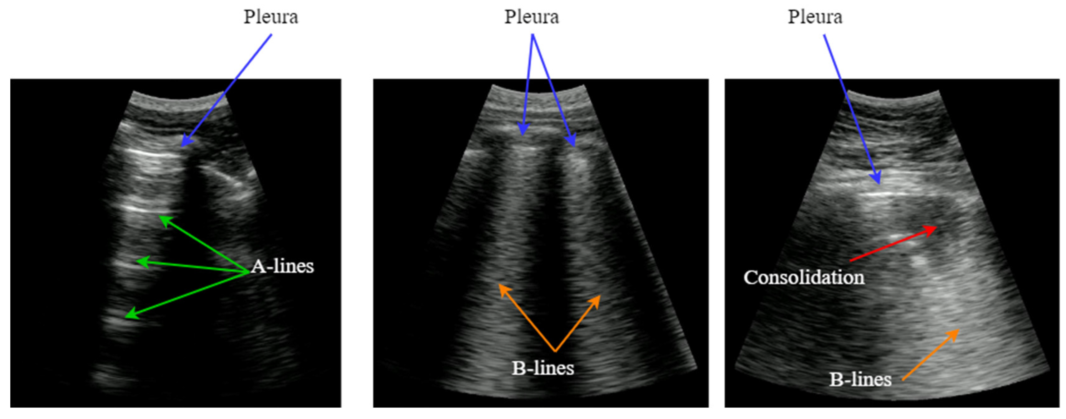
As the disease advances, more air is substituted by liquid and then consolidates into solid material. These consolidations appear in the image as hypoechoic regions, and constitute the third artifact usually looked for when imaging the lung. In sum, artifacts like A-lines, B-lines and consolidations, are indicative of the lung condition, and can be used to diagnose a pulmonary pathology [4]. Detecting and interpreting these artifacts is the key for a correct evaluation of lung images, which has been the principal bottleneck in the dissemination of this technique.

Moreover, the shock caused by the COVID-19 pandemic amplified the relevance of pulmonary ultrasound as a vital tool for evaluating pulmonary conditions. As the pandemic disseminated worldwide, LUS emerged as a frontline modality for assessing lung involvement and monitoring pulmonary condition, particularly in patients affected with COVID-19 pneumonia. Its real-time, bedside capabilities offered rapid insights into lung pathology, especially in emergency, critical care units and domiciliary attention, where other imaging modalities like TAC and magnetic resonance encountered limitations or were less accessible [1,5,6,7,8].

In this context, the integration of diagnostic aid algorithms into ultrasound scanners could help reduce the learning curve of the technique, as well as reducing the evaluation time and possible increasing the diagnosis success. Artificial intelligence (AI) has brought about significant advancements across diverse scientific and medical fields, showcasing its potential in reshaping the landscape of diagnosis and patient welfare. Within the realm of healthcare, AI is revolutionizing the field, showcasing promising outcomes through the provision of sophisticated tools that aid healthcare providers in making clinical decisions. This integration has led to improvements in precision and effectiveness, enhancing the process of diagnosing and treating a wide range of medical conditions [9].

Several authors propose the application of AI-based algorithms with ultrasound lung images, for addressing the challenges related with artifacts identification and quantification. There are usually two different approaches to this problem: Processing a whole ultrasound video and classify it according to the disease severity, or processing the video frame-by-frame, highlighting the artifacts that are found by labeling the image. The first approach means a classification problem, where the input is a buffer of images, and the output is a severity score. The second one is a segmentation problem, where visual feedback is given to the clinician about the type, position and extent of the imaging artifact. In this work we propose to combine both, providing frame-by-frame real-time identification and enhancement of artifacts, along with a score of the whole video based on the artifacts found.

In [10] the authors propose a deep learning solution capable of assigning a severity score to a lung ultrasound video. They pose the problem as a classification problem where the network learns to assign a score based on the artifacts found in the input to the network. In [11] the authors design an algorithm to extract from a lung ultrasound video several images that serve as a summary of the ultrasound examination. These images are subsequently introduced to a neural classification network to assign a score. So here the network goes on to evaluate the classification problem on an image-by-image basis. In case of [12] the authors combine CNN with Long Short-Term Memory (LSTM) networks to extract special and temporal features to classify between healthy and non-healthy at video level.

If we talk about image-by-image processing, in [13] the authors propose a deep learning model for B-line detection trained on images from Dengue patients as a classification problem. In [14] different solutions for B-line detection and localization are proposed: as a video-level and frame-level classification problem and as a frame-level segmentation problem. The authors conclude that frame-by-frame segmentation has an advantage over the other solutions because it results in less variability in image interpretability by different physicians. Other works such as [15] focus on the detection of B lines by visualizing the activation map on the output of a binary classifier convolutional network. Here they contemplate the possibility of using such solutions in real time.

The above mentioned works focus on the detection of a single artifact, the B lines, which means that other solutions are needed for the other artifacts typical of pneumonia and lung ultrasound. In [16] instead, a multiclass segmentation model that distinguishes multiple artifacts is proposed, but unlike our work, the model is trained with images obtained from a lung phantom.

2. Methods

2.1. Neural Network Architecture

Convolutional Neural Networks (CNNs) find extensive usage in real-time segmentation tasks due to their capability of recognizing local patterns and characteristics within images. They provide processing efficiency and a hierarchical feature structure enabling the identification of both intricate details and broader patterns. Specifically, the U-Net architecture stands out for its specialization in semantic and medical segmentation [17]. Its skip connections facilitate the fusion of information across various spatial scales, resulting in the creation of highly detailed segmented masks. This is particularly advantageous in medical imaging, like lung consolidation segmentation.

With the aim of improving the behavior and response of our model, various U-Net network modifications were studied, customizing the U-Net architecture using the python library Keras-unet, developed by K. Zak and published on GitHub [18]. Finally, the chosen architecture is Attention U-Net developed by O. Oktay in [19] where attention gates filters are added in the decoder part, which automatically learns to focus on main patterns with different shapes and sizes, improving the result of the prediction. In order to find a compromise between computational cost, performance and network complexity, we chose to use 16, 32, 64 and 128 filters on the encoding layers respectively and the inverse for the decoding layers. Higher filter counts increase the model’s complexity and resource needs significantly, which may not translate into better performance for our task.

Two implementation options were explored with the aim to see what is more suitable for the described problem: A different model for each pneumonia pattern, and a single model capable of predicting and segmenting all main lung ultrasound patterns (Pleura, A-line, B-line, Consolidation). Both solutions present advantages and disadvantages which were taken into account. The use of several models offer a more specific response and the possibility to tune the network according to each pattern to get the best behavior, but, on the other hand, using several models the inference time increase, making the real-time implementation more difficult. While using one global network with multiple outputs, the response could be less precise if we compare each output with a network specifically trained for that pattern, but the main advantage is that the inference time is reduced allowing a real-time implementation.

2.2. Dataset

The data used to perform this study was obtained in the clinical trial ULTRACOV [20]. It was generated with a 128-channel ultrasound electronic equipment developed in-house, and a medical grade 3.5 MHz convex probe. A total of 689 videos were acquired, corresponding to 30 patients and following a standardized scanning procedure of 12 thoracic regions [21].

The videos were manually annotated by an expert physician, indicating the presence or not of each artifact in the video. Then a score for the patient was calculated, taking into account the videos of the 12 scanned regions. Because the videos where not labeled frame-by-frame by the expert, a semi-automated annotation algorithm was developed (Section B.2).

2.3. Neural Network Input Data

The format of the input data has a great impact on the deep learning model definition and performance. A typical ultrasound image with a curved array (like that used in this study) is a circle sector, defined by an aperture angle α, an initial range r₁ and a final range r₂, which is usually framed into a rectangular image with size WxH pixels (Figure 2.Left). But, in fact, a sector ultrasound image is originally formed by N scan lines usually equal distributed inside the sector area. These lines, containing M samples each, are the output of the beamforming algorithm, and could be interpreted themselves as a rectangular image (Figure 2.Right).

The algorithm to get the sector image from the B-Scan data is usually called scan-converter, and it is typically implemented by bi-linear interpolation of the acquired samples over the pixel grid. This process is carried out by the scanner, which gives the user the sector image in WxH format. Therefore, a question arises about which image format is more appropriate for implementing the deep learning algorithm aimed in this work.

Sector image has the advantage of being more easily accessible, because it is the typical output format on most ultrasound equipment. Therefore, it maintains the aspect ratio of the structures to be imaged, which eases interpretation by medical professionals. However, accommodating a sector image inside a rectangular grid generates black margins around it, which besides adding pixels with no information, could potentially introduce a bias in the automated image analysis. Furthermore, the shape and extension of these zones depends on the scanner model and configuration, hindering the translation of the resultant model between different scanners.

On the other hand, rectangular B-scan images have the advantage of providing only useful information (no black margins), while its rectangular format is highly suitable as input for segmentation models. Another important advantage is that each vertical line represents a physical propagation direction of the beam inside the tissue, which is particularly relevant for artifacts like B-Lines, that appears precisely on those directions. Therefore, a B-Line will be always seen in the B-Scan as a vertical artifact, independently on its position on the pleura, and of the scanner configuration. Furthermore, scanner configuration parameters like the aperture angle α or the initial and final range r₁ and r₂ only affect the size MxN of the image, which simplifies adapting images acquired by different equipment to the same network, only by vertical and horizontal scaling. On the other hand, these images are not suitable for visual interpretation, as they present a distorted view of the tissue anatomy. Because not all ultrasound equipment provides direct access to B-Scan data, a Sector-Image-to-B-Scan conversion algorithm would be needed. With a similar approach than scan-converter algorithms from B-Scan to sector image, it could be based on a simple bilinear interpolation algorithm, after defining a set of beam lines that cover the useful area of the sector image (green lines in Figure 2.Left). In this work, we had access to the B-Scan raw data generated by our system, so no Sector-Image-to-B-Scan process was needed.

Furthermore, for possible future hardware implementations of the proposed models, using B-scan data would be optimal in the sense that it reduces the amount of information to be processed, and uses data in a raw format available at low hardware level.

For defining the size of the B-Scan images, the typical number of beams in an ultrasound scanner has to be taken into account. For convex probes like the one used in this work, an active sub-aperture is used for generating each beam, with typically between 32 and 64 elements. That sub-aperture is moved along the array in one or several elements step, forming the B-Scan. For example, a 128 elements array with a 32 element aperture can generate up to 96 scan lines, while a 196 elements array with an aperture of 64 elements generates 132 scan lines. Based on these typical numbers, an input width of 128 lines was selected, being power of 2 for operations optimization.

The size of the vertical direction is related to the frequency content of the signal and the sampling rate. For an ideal 100% bandwidth array, the maximum frequency content of the signal envelope is equal to half the array center frequency. To reconstruct the envelope without aliasing, the pixel density in the vertical direction should be, at least, able to sample the signal at double of that frequency (Nyquist criteria). For the array used in this work with 3.5 MHz center frequency and 70% bandwidth, the number of pixels required for sampling up to 70 mm and 90 mm is 210 and 294 respectively. Based on these numbers, a height of 256 was selected for the network, which imposes a trade-off between training and inference cost and image quality. In case that larger images are used, they should be scaled down using compression algorithms that preserve the artifacts information. For example, in the scanner used in this work, a data reduction algorithm without peak information losses is available [22], and was used to accommodate the B-Scan height to the network size. In Figure 3, a comparison example between sectorial and B-scan images is shown.

2.4. Neural Network Output Data

2.4.1. Labelling Tools

One of the limitations of the used dataset [20] is that it was labeled by an expert physician at video level, while for training a segmentation network, it has to be labeled at frame level. While asking a physician to label frame-by-frame such a large dataset is usually impractical, a semi-automated algorithm was developed for this task, based on the initial label of the presence of each artifact in the video. Depending on the type of artifact this process if fully automated or requires to identify a key frame where the artifact is visible and manually segment it, being then automatically followed throw the subsequent frames in the video. These algorithms are explained in the following subsections.

2.4.1.1. Pleural Line Labelling

One of the most important indications to identify in a lung ultrasound image is the pleura, because it defines the zone where the artifacts have to be looked for. Correctly identifying the pleura helps to discard zones that do not have to be analyzed, like the ribs and their shadows and the muscle and fat area above it. Giving this information to the neural network could improve the results, as it will learn that the B-Lines and consolidations are located bellow the pleura, and not in other areas of the image.

The algorithm for automatically segmenting the pleura is based on the fact that, when the ultrasound probe remains stationary, the image above the pleura (fat and muscle) remains basically unchanged between frames, while variations in the image occur below the pleura due to the respiratory cycle. Then, by subtracting consecutive frames, an auxiliary image is formed, where the upper region is almost black, and the lower part is bright. Furthermore, if several of these images are averaged, the random nature of the speckle in the lower part generates a quite homogeneous region that can be more easily distinguished from the upper region. The frontier between these regions can be considered a first approximation of the pleura line.

Given a video V formed by K frames B defined by

V = \{B_{1}, B_{2}, \dots, B_{K}\}

(1)

where

B_{i} = [b_{i} (m, n)] \in R^{M x N} f o r 1 \leq i \leq K, 1 \leq m \leq M a n d 1 \leq n \leq N

(2)

and b_i,(m,n) is the pixel intensity of image i at position (m,n), the output of the proposed algorithm is

\tilde{V} = \{{\tilde{B}}_{1}, {\tilde{B}}_{2}, \dots, {\tilde{B}}_{K - L}\}

(3)

where

{\tilde{B}}_{i} = \frac{1}{L} \sum_{k = i}^{k = i + L - 1} |B_{i + 1} - B_{i}|

(4)

being L the length of the averaging filter. Figure 4 shows an example output of the algorithm. On the left is the original B_i image of a frame, and on the right its filtered version V_i, showing the two formerly mentioned dark and bright zones. For detecting their boundary, a dynamic threshold was applied to each vertical line of the filtered image, calculated from the average amplitude of the upper part of the image:

{\tilde{P}}_{j} = m i n \{i | A_{j} (i) > {t h}_{j}\}

(5)

where

A_{j}

is the vertical line of the filtered image at column j,

{\tilde{P}}_{j}

is the vertical index to the pleura guess for that line and th_j the applied threshold. Figure 4.b shows with green dots an example of this set of initial pleura raw guess points

{\tilde{P}}_{n}

, which are then used to fit a second order polynomial to obtain a smooth representation

P_{n}

of the initial guess (red line in Figure 4.b).

It is worth to mention that directly applying a threshold to the original image (Figure 4.a) is very prone to misdetections, as other horizontal bright lines in the upper region of the image are present, with pixel intensity values even larger than those of the pleura. On the other hand, the auxiliary image filtered by the proposed method is very suitable for a simple threshold detection, because of its stepped nature.

This first approximation does not take into account that a bright line has to be seen in the image to be considered part of the pleura line. Then, the P_n indexes are used as the center of a vertical window with W samples, where to look for the maximum amplitude of the original image. If this amplitude is larger than a global threshold T, it is considered that the pleura is present in the window. Then, a -3dB signal drop criteria is used to find the high amplitude zone around the maximum, and those pixels are labeled as belonging to the pleura in a binary mask called M. The mathematical formulation of this part of the algorithm is as follows:

M_{i} (m, n) = \{\begin{matrix} 1, i f b_{i} (m, n) \geq A_{m a x} (m) \cdot 10^{- \frac{3}{20}}; f o r n \in [{\tilde{P}}_{j} - W, {\tilde{P}}_{j} + W] \\ 0, o t h e r \end{matrix}

(6)

Keeping the previous nomenclature, this condition checks if the amplitude at position (m, n) remains within 3 dB of the maximum amplitude at

{\tilde{P}}_{j}

(

A_{m a x})

which corresponds to an approximate 29% drop in amplitude. If this condition is met, the pixel is considered part of the pleura and is marked as 1 in the binary mask. Otherwise, it is marked as 0. For this particular dataset, the approximation is applied in a searching window W=20 samples around the pleura maximum amplitude identified in each scan line, but W should be adjusted according to the image resolution to include a region of about 6 mm around the pleura.

Finally, morphological opening and closing filters sized at 3x3 are applied to refine and smooth the pleura labeling mask (Figure 5.c), eliminating outliers and giving a more precise representation of the higher amplitude line. For each video, a set of K-L pleura binary mask images are generated, to be used during the training process of the network.

2.4.1.2. A-Line Labelling

In case of A-lines, the developed algorithm detects these patterns as echoes of the pleura occurring at depths that are multiples of the probe-to-pleura distance. A search window W

[w_{1}, w_{2}]

is applied at those depths to find signal peaks that cross a threshold, and then verify their validity by comparing with the average amplitude in consecutive lines:

a_{j} = \arg \underset{x \in [w_{1}, w_{2}]}{m a x} A_{j} (x)

(7)

where

a_{j}

corresponds to the index in the A-scan signal

A_{j}

where the maximum amplitude is located within the window

[w_{1}, w_{2}]

, which corresponds with an initial guess of the A-Line position.

As in the case of the pleura line, to define the ground truth mask, a -3db signal drop criteria equivalent to the formula 6 is used, followed by the application of opening and closing morphological filters sized at 3x3 to refine the mask and eliminating outliers.

2.4.1.3. B-Lines Labelling

The approach employed to recognize these pneumonia indicators involves fitting each A-scan line

A_{j}

within the image to a linear function

y (x)

that initiates from the identified pleural line representing the amplitude of the signal at a depth

x

y (x) = m \cdot x + d

(8)

where

m

is the slope and

d

is the intercept. Then several thresholds are stablished to confirm the detection of the B-line based on a maximum slope

S_{t h}

, standard deviation

σ_{t h}

and average amplitude of the signal

A_{a v g t h}

after the pleural line detected. Therefore, the lines considered as B-line

{B l}_{j}

are calculated as follows, as a boolean vector with length n (number of lines):

B l_{j} = \{\begin{matrix} T r u e, i f m > S_{t h} a n d σ {< σ}_{t h} a n d A_{a v g} > A_{a v g t h} \\ F a l s e, o t h e r s \end{matrix}

(9)

Once the A-scans with B-lines are known, the annotated masks are generated marking B-lines region below the pleura line frame by frame.

2.4.1.4. Consolidation Labelling

While pleura, A-lines and B-lines can be robustly detected by quite simple algorithms applied along each scan line, the consolidations cannot be tackled with the same approach. As they are intrinsically two-dimensional structures, it is not possible to detect them in a line-by-line basis, and image algorithms are needed.

The approach followed in this work was that, given a video labeled by the expert as containing a consolidation, a key frame where this consolidation is seen is first identified. Then, it is manually delineated using a custom developed interactive tool (Figure 6). Finally, an optical flow algorithm [23,24] tracks the movement of the consolidation in the subsequent frames, automatically generating the ground truth masks for the entire video. The optical flow algorithm is based on the principle of selecting a set of reference points and track them through the video. This algorithm is particularly suited for ultrasound images because the texture generated by the image speckle can be used for this purpose. The implemented application requests frame-by-frame validation from the user to ensure correct labelling. In case the algorithm fails in the detection, the points of interest will be re-selected again.

These semi-automatic algorithms are aimed to decrease the time required for labelling videos at frame level, while they only require manual intervention in the case of consolidations and for segmenting a unique frame. Nevertheless, because they can also fail in detecting the indications, a supervision of the whole video after it is labeled is required, with the possibility of eliminating those frames where the labeling is considered wrong.

2.4.2. CNN Output

The output of the network proposed in this work, instead of a multiclass segmentation, adopts a multi-output binary segmentation approach, with each output dedicated to a distinct artifact: Pleura, A-line, B-line and consolidation. This strategy ensures a more accurate delineation of boundaries unique to each artifact, avoiding the risk of predictions blending or obscuring one another within the image, and facilitating identification and classification of multiple artifacts simultaneously.

Consequently, the network will output 4 binary masks, with a size of 128 x 256 pixels each, corresponding to each artifact studied in this work.

2.5. Training

The proposed network was trained with a database of 689 annotated videos from a clinical trial involving 30 patients [19], which were processed with the semi-automated labeling algorithms presented in the previous section. The selection criteria for each training step is as follows:

Among the 30 patients, 27 were chosen for training the model. The videos of these patients contained images of all the artifacts to be detected, to ensure maximal learning for the model. The remaining videos were reserved for a final validation phase to perform an extra verification of the model’s behavior. Since consecutive frames in a video often have a close resemblance, the K-means clustering algorithm [25,26] was applied to select the most distinctive images from each video: similar frames are grouped into clusters, and the frames closest to the centroids of these clusters are selected as key frames, avoiding overfitting during training. In this study, 3 key frames were selected per video.

Additionally, data augmentation methods, including image saturation with random gain values and the introduction of horizontally flipped images, were utilized (Figure 7). Image saturation is particularly important in ultrasound imaging because the gain control is arbitrarily adjusted by the physician during the examination, based on their eye perception. Therefore, in some high-gain images the pleura line can be artificially thickened by saturation, and the model should learn to identify it, even in that scenario. Furthermore, detection of B-Lines should be based on their shape and variation along the scan line, but not on their absolute amplitude, which can be induced by introducing images with different gains but correctly labeled. These techniques are aimed to enhance the model’s adaptability to differences in ultrasound image gain, and to introduce greater image variability.

The application of these criteria resulted in a dataset comprising 9159 annotated images, which were randomly divided into 70% for training and 30% for test.

Training was carried out using 2 NVIDIA 2080 TI in parallel, applying dropout=0.3 to avoid overfitting during the process, as well as a binary cross-entropy loss function being 100 the number of epochs, 64 the size of the batches and a learning rate of

{5 x 10}^{- 4}

2.6. Validation

An important step in the development of solutions with artificial intelligence tools is validation, which involves assessing the model’s performance on data that was not used during training to ensure that it can generalize well to new unseen examples. Validation is crucial for identifying overfitting, where a model performs well on the training data but fails to generalize to other datasets. For this work, validation is conducted at frame and video level.

At the frame level, a frame-by-frame check is performed to observe how well the prediction align with the ground truth. Several metrics such as Dice coefficient, IoU, recall, precision, and F1 score have been calculated, and the average value for each artifact (pleura, consolidations, A-lines, and B-lines) has been determined.

Additionally, to achieve a more thorough validation of the model’s behaviour, video-level validation is performed. This involves comparing the presence of artifacts detected by the algorithm with the opinion of an expert clinician, ensuring a holistic evaluation of its diagnostic accuracy. Besides highlighting the artifacts in each frame with the segmentation model, a global indication for the findings on the whole video would also be valuable for the physicians, in order, for example, to calculate a score of the global condition of the patient. In this sense, two different validations were conducted. First, the reliability of the method was tested with all the acquisitions from the database. Second, the software's performance is verified on videos of patients not included in the training set, as explained in Section C. The results of the various validation tests are presented in Section VI of the results.

2.7. Implementation of the Solution

To achieve real-time processing of the ultrasound images received from the scanner, an asynchronous architecture based on parallel processing was developed. This approach facilitates seamless communication among different processes, ensuring a continuous and responsive workflow. The implementation was carried out using the Python programming language, and libraries that streamline real-time image rendering, such as Pyqtgraph [27].

The development comprises two primary parallel processes: a main process responsible for receiving ultrasound data and a secondary process dedicated to processing the received information and delivering real-time responses. Both processes are supported by rendering functions that update the user interface to ensure smooth visualization of the results. Figure 8 illustrates the proposed architecture, and each block is explained in detail in the following sections.

2.8. Main Process

The main process is responsible for receiving real-time images from the scanner via a TCP communication channel. The received data is decoded, extracting essential information such as frame identifier, number of samples, number of lines, and the B-scan data. This data is then passed to the real-time info object to be shared with the other processes, which are notified by setting different work-flow flags.

2.9. Real-Time Computing Process

This process remains latent, awaiting the reception of images to be processed. Real-time processing involves multiple pre-processing steps before applying the trained deep learning model and various post-processing algorithms to enhance system response. The processing flow is illustrated in Figure 9, and it is explained below.

2.9.1. Pre-Processing Block

Pre-processing algorithms are carried out before executing the Deep Learning model. These algorithms serve as a preliminary filtering steps to avoid processing images that do not meet the quality criteria for evaluation. First, probe movement is verified, because acquisitions where the probe is not held still cannot be analyzed. Using optical flow algorithms [23,24], probe movement is estimated between two consecutive images, using reference points located in the upper part of the image (muscle and fat). A movement threshold of 2 mm/s was established. If the image does not meet the criteria, it is not processed, and it will be displayed on the screen with a red label indicating movement (see in Figure 12.d). If, on the contrary, it meets the requirements, a green label will be displayed on the screen (Figure 12.c) and the rest of the processing will be executed.

2.9.2. Model Prediction

Only if the pre-processing criteria have been met, the inference of the artificial intelligence model is performed. As explained in previous sections the inference is conducted frame by frame as soon as the real-time process is free, and then 4 different binary segmentation mask are obtained: pleura, consolidation, a-lines and b-lines.

2.9.3. Post-Processing Block

After inference, several steps are performed on the output to improve robustness. First is verified whether the pleura has been detected or not, as the presence of A-Lines, B-Lines and consolidations becomes unreliable if the pleura is not detected. Correct detection of the pleura is a differentiating factor for the accurate interpretation of the image.

2.10. Communication Between Processes

One of the key components of real-time development is the communication between different processes. To achieve this, a base manager object from the Python multiprocessing library [28] is used. This object allows customizing a shared object with the necessary fields to carry out the various functions of the code. The manager serves as a bridge between different processes and, through the use of flags that act as locks, allows manipulation of the different fields without compromising the application's fluidity and avoiding deadlocks.

2.11. Visualization

Two single-shot timer are programmed, one for the real-time representation of ultrasound images, and another for the rendering of predictions. This approach ensures that both renderings operate independently, without compromising real-time performance. As soon as both timers have new content to render, it will be displayed on the screen.

Figure 10 shows the screen shown to the user. On the left, the acquired sector-scan images are shown in real-time, with several overlays coming from the processing algorithm. When the image is valid for being evaluated, the contour of the image turns green, and so the label “movement” on the upper right corner. If the image fails to pass any of this criterion, the contour line turns red, and so the labels that triggered the event. Therefore, the physician can freely move the probe on the patient chest until theses indications turn green, and then hold probe steady to acquire a video of 3 seconds that will be saved for each of the 12 regions to be examined according to the protocol.

This image also overlays, in real-time, the findings of the neural network. The pleura is marked with blue points, A-Lines with green points, B-Lines with orange points and consolidations with red points. Furthermore, a series of statistics and messages are shown in the lower part of this image: The percentage of frames with A-Lines in the last 6 seconds, the number of isolated B-Lines, calculated as the sub-regions with an average 6dB drop in the angular direction within the region where B-Lines were detected, the percentage of the affected pleura calculated as the number of scan lines affected by B-Lines over the total number of scan lines where the pleura was detected, and a label in red indicating that a consolidation when present.

On the right of the screen an image we refer as pleura C-scan is shown. The C-Scan is a type of image widely used in Non-destructive Testing (NDT) applications where B-scan images are acquired while the probe is moving and a visual representation of the whole component is needed [29]. For each image line within the B-Scan, the maximum amplitude is obtained within a gate at some depth, which ensembles an image that can be interpreted like a top view of the component, with defects information at a certain depth. We adapted this concept using a gate at the depth of the pleura, obtained from the pleura mask given by the model, and substituting the mechanical movement of the probe in an NDT scan, by the time index in the acquired video. Therefore, each horizontal line in the pleura C-Scan correspond to a frame in the video, and it shows the brightness of the pleura line along the horizontal dimension of the image. At each of these lines landmarks with the previously defined colours are also plotted. As the video progresses, the C-Scan image is constructed frame by frame from top to bottom and, at the end, all the relevant information of the video is condensed in only one image. The presence of A-Lines, B-Lines and consolidations and their extension with regard to the pleura width can be appreciated, and also the pleura sliding effect as the indications move laterally during the scan. Furthermore, these images could be saved for each acquired region in the chest, and shown in a single panel that depicts the global condition of the lung in a single view, without the need to review each of the acquired videos for the whole examination, which could help to reduce time during follow up of patients.

3. Results

In this section the results obtained in the study are shown, regarding the behaviour of the trained neural network and the results of the real time implementation. Metrics and values calculated on the 2 different datasets mentioned in validation section are shown: on the test set of 2748 images, and on a second validation set using images belonging to the 3 patients that were not used during the training stage.

3.1. Model Results

As explained in the validation section, a study was conducted to validate the model's response frame by frame. The results are presented in Table 1, Table 2, Table 3 and Table 4, where the Dice coefficients, Intersection over Union (IoU), F1-score, recall, and precision values are calculated. Figure 11 shows the behaviour of the model applying different thresholds to the network output showing the mean values of the metrics in the test dataset. Given the stability of these results, it makes sense to apply 0.5 as a generic threshold to the network output.

It is interesting to note in Table 1, Table 2, Table 3 and Table 4 how the results, between patients included in the training and not, present a similar behaviour. The network, despite the fact that in both cases are images that have never seen, is able to match more accurately in data from known patients (Table 1 and Table 2). However, the results shown in Table 3 and Table 4 suggest that the neural network has been able to generalize the problem and maintain high success rates.

Figure 12 shows different network output examples modifying the saturation of the image at the input of the network, to simulate the gain variation usually applied on an ultrasound scanner. Segmentation and detection of artifacts remains stable, guaranteeing correct operation in spite of signal saturation.

Figure 12. Results comparative with different image gain: a) healthy lung; b) pathological lung; c) grave lung.

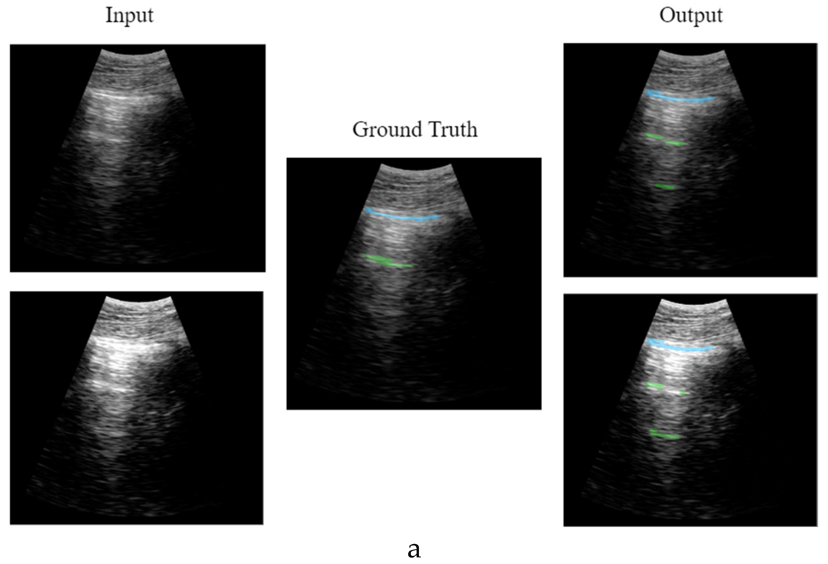
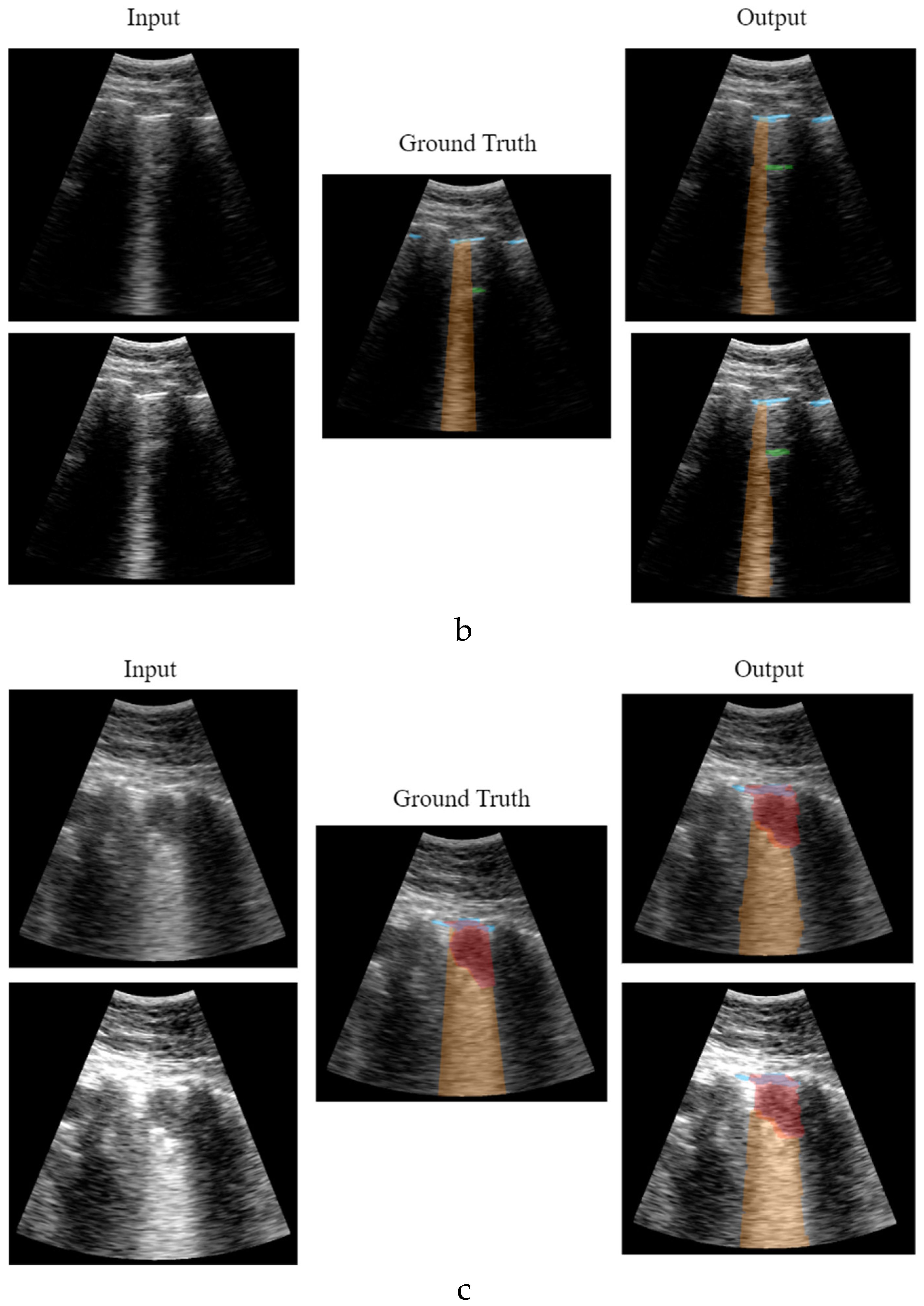
Figure 12.a shows the learning and generalization capacity of the trained model. The labelling algorithms of the A-line only considers a single A-line at double the distance between the probe and the pleura; however, the model is able to detect the second and even the third echo in some particular cases, demonstrating the capacity of the model in generalizing and learning the problem. It is worth to mention that this fact negatively affects the validation metrics calculated in Table 2 and Table 4, where the false positive values for A-lines are higher. This is because the second and third occurrences of the A-lines are not labelled in the input dataset, which is a limitation of the labelling algorithm rather than of the model itself.

3.2. Real-Time Implementation Results

As already mentioned, the implemented software is able of processing and displaying in real-time the pleural line, B-lines, consolidations, and A-lines. The algorithm can calculate and obtain the percentage of pleura affected by B-lines, which could be useful to physicians when classifying and determining the severity of a patient’s condition.

The implementation proposed in this study achieves a processing rate of up to 20 predictions and image update per second using an octa-core i5 CPU processor and a NVIDIA GeForce RTX 2060 GPU, which is a medium-range hardware set-up. This figure coincides with the frame-rate given by the ultrasound scanner, so we can state that the solution operates in strict real-time. In terms of computational cost in the different processes, the main process takes about 10ms, which gives a fluid and latency-free feeling during the scan, while the real-time computation process takes about 50ms of which 20-25ms is for model inference on the GPU. It is worth to mention that the final image refresh rate depends on the number of artifacts detected, due to the respective post-processing and painting algorithms which are not yet optimized. Therefore, the effective frame rate obtained was between 17 and 20 FPS,

Regarding prediction capability at the video level, the results given by the model are compared with the opinion of an expert physician. Two different calculations are performed: first, its performance with the test dataset is assessed (Table 5), and second, a specific comparison is made for the set of patients excluded from training (Table 6). With these results it is worth noting that the number of false positives and false negatives are balanced in the case of detection of consolidations and B-lines, which is positive since it is a sign that there is no bias in the training.

It can be observed that the accuracy of the proposed solution at the video level is quite high and it behaves stably even with patients out of training. In the case of the detection of A lines, the results are notably worse than for consolidations and B-Lines, and this because in the labelling process carried out by the physician in [20] labelling the A lines was not mandatory, given that they are indicative of healthy lungs. Therefore, the dataset labelling contains false negatives in those videos where the A-Line is present, but it was not marked by the physician. This is a limitation of this study, but it does not imply that the performance of the solution is nevertheless promising.

Figure 13 shows several examples of the screen of the implemented software in operation explained in Section F.4.

4. Discussion

The implementation of software solutions using deep learning algorithms is a step towards assisted diagnosis in lung ultrasound. Both the model and the complete solution demonstrate solid performance, validated by the results shown in the previous section. Based on studies such as [30], which demonstrate the variability in physicians' opinions, and taking into account that the proposed method works in real-time (up to 20 fps), it could be a useful tool for clinical practice, helping physicians to quickly address lung conditions and reducing the learning curve for less experienced healthcare personnel in the field.

Despite the promising results, there are some limitations in this work that require further research. One of the main ones is the limited extent of the database used to train the model. Only 689 videos from 30 patients are available, which are insufficient to obtain a fully trained model capable of generalizing the entire problem across the four artifacts sought. For example, in the case of videos with consolidations, only 58 out of the total of videos exhibit that artifact, which also explains the high values shown in Table 1. It should also be highlighted that the images used in this study belong to a single scanner, which is likely to be a limitation given the unique image characteristics of each equipment in terms of noise, sampling frequency, etc. which may introduce bias to the network training.

Another limitation of the implemented model lies in its inability to always segment the complete B-line. In some cases, only part of the B-line is segmented as is shown in Figure 14. This behaviour is corrected by the post-processing algorithm, which marks the whole scan line as affected by B-line regardless the vertical extension of the output mask. Therefore, the results shown in Table 5 and Table 6 are not affected by this phenomenon, but it indicates that there is already some improvement margin in the network definition and/or in the training process.

For future work, these limitations could be addressed including new data into the training, or applying transfer learning technics to adapt the result to other scanners, to get a more scalable solution. New modifications to the network architecture could be also studied to improve the behaviour of the model, as well as implementing in FPGAs, for enhancing its adaptability to broader clinical scenarios.

5. Conclusions

In this study, we have shown the effectiveness of employing deep learning models along with signal processing algorithms for accurate detection of pleura, A-lines, B-lines and consolidations in lung ultrasound images. The proposed model has been developed as a help for assisted diagnosis, demonstrating promising capabilities in accurately segmenting and detecting key features in the images.

The proposed implementation exhibits efficient real-time processing capabilities with moderate hardware resources, achieving a rate of up to 20 predictions per second in a mid-range computer. This makes it suitable for application in clinical settings, where timely diagnosis is crucial for patient care. While the results are promising, this solution presents opportunities for future research and improvements in model and architecture design.

The use of semi-automatic labelling tools could be helpful when working with large amounts of data. Frame-by-frame labelling is a time consuming task, which cannot be always performed by expert physicians in a fully manual way. In terms of segmentation accuracy, the trained model obtained DICE values of 83% for pleura, 96% for consolidations, 87% for B lines and 62% for A lines. These results suggest that solutions of this type could be used in clinical environments, to reduce subjectivity in the interpretation of images, and even as a tool to help less experienced physicians to perform lung echography and reduce the learning curve of the technique.

Acknowledgments

This research was partially supported by the project PID2022-143271OB-I00, founded MCIN/AEI /10.13039/501100011033 / FEDER, UE and by the fellowship PRE2019-088602 founded by MCIU (Spain).

References

Ferreiro Gómez M, Dominguez Pazos SJ. The Role of Lung Ultrasound in the Management of Respiratory Emergencies. Open Respir Arch. 2022 Sep 13;4(4):100206. [CrossRef] [PubMed] [PubMed Central]
Hansell L, Milross M, Delaney A, Tian DH, Rajamani A, Ntoumenopoulos G. Barriers and facilitators to achieving competence in lung ultrasound: A survey of physiotherapists following a lung ultrasound training course. Aust Crit Care. 2023 Jul;36(4):573-578. Epub 2022 Jun 7. [CrossRef] [PubMed]
G. Soldati, A. Smargiassi, L. Demi, and R. Inchingolo, “Artifactual lung ultrasonography: It is a matter of traps, order, and disorder,” Applied Sciences, vol. 10, no. 5, p. 1570, Feb 2020. [CrossRef]
Bhoil R, Ahluwalia A, Chopra R, Surya M, Bhoil S. Signs and lines in lung ultrasound. J Ultrason. 2021 Aug 16;21(86):e225-e233. Epub 2021 Sep 9. [CrossRef] [PubMed] [PubMed Central]
Tung-Chen, Y.; Martí de Gracia, M.; Díez-Tascón, A.; Alonso-González, R.; Agudo-Fernández, S.; Parra-Gordo, M.L.; Ossaba-Vélez, S.; Rodríguez-Fuertes, P.; Llamas-Fuentes, R. Correlation between chest computed tomography and lung ultrasonography in patients with coronavirus disease 2019 (COVID-19). Ultrasound. Med. Biol. 2020, 46, 2918–2926. [CrossRef]
Vieillard-Baron A, Goffi A, Mayo P. Lung ultrasonography as an alternative to chest computed tomography in COVID-19 pneumonia? Intensive Care Med. 2020 Oct;46(10):1908-1910. Epub 2020 Aug 25. [CrossRef] [PubMed] [PubMed Central]
Demi, L., Wolfram, F., Klersy, C., De Silvestri, A., Ferretti, V.V., Muller, M., Miller, D., Feletti, F., Wełnicki, M., Buda, N., Skoczylas, A., Pomiecko, A., Damjanovic, D., Olszewski, R., Kirkpatrick, A.W., Breitkreutz, R., Mathis, G., Soldati, G., Smargiassi, A., Inchingolo, R. and Perrone, T. (2023), New International Guidelines and Consensus on the Use of Lung Ultrasound. J Ultrasound Med, 42: 309-344. [CrossRef]
Gil-Rodríguez J, Pérez de Rojas J, Aranda-Laserna P, Benavente-Fernández A, Martos-Ruiz M, Peregrina-Rivas JA, Guirao-Arrabal E. Ultrasound findings of lung ultrasonography in COVID-19: A systematic review. Eur J Radiol. 2022 Mar;148:110156. Epub 2022 Jan 20. [CrossRef] [PubMed] [PubMed Central]
Amisha, Malik P, Pathania M, Rathaur VK. Overview of artificial intelligence in medicine. J Family Med Prim Care. 2019 Jul;8(7):2328-2331. [CrossRef] [PubMed] [PubMed Central]
Mento, F.; Perrone, T.; Fiengo, A.; Smargiassi, A.; Inchingolo, R.; Soldati, G.; Demi, L. Deep learning applied to lung ultrasoundvideos for scoring COVID-19 patients: A multicenter study. J. Acoust. Soc. Am. 2021, 149, 3626–3634. [CrossRef]
Khan, U.; Afrakhteh, S.; Mento, F.; Mert, G.; Smargiassi, A.; Inchingolo, R.; Tursi, F.; Macioce, V.; Perrone, T.; Iacca, G.; Demi, L. (2023). Low-complexity lung ultrasound video scoring by means of intensity projection-based video compression. Computers in Biology and Medicine. 169. 107885. [CrossRef]
Barros B, Lacerda P, Albuquerque C, Conci A. Pulmonary COVID-19: Learning Spatiotemporal Features Combining CNN and LSTM Networks for Lung Ultrasound Video Classification. Sensors. 2021; 21(16):5486. [CrossRef]
Kerdegari, H.; Phung, N.T.H.; McBride, A.; Pisani, L.; Nguyen, H.V.; Duong, T.B.; Razavi, R.; Thwaites, L.; Yacoub, S.; Gomez, A.; et al. B-Line Detection and Localization in Lung Ultrasound Videos Using Spatiotemporal Attention. Appl. Sci. 2021, 11, 11697. [CrossRef]
Lucassen, R. T., Jafari, M. H., Duggan, N. M., Jowkar, N., Mehrtash, A., Fischetti, C., Bernier, D., Prentice, K., Duhaime, E. P., Jin, M., Abolmaesumi, P., Heslinga, F. G., Veta, M., Duran-Mendicuti, M. A., Frisken, S., Shyn, P. B., Golby, A. J., Boyer, E., Wells, W. M., … Kapur, T. (2023). Deep Learning for Detection and Localization of B-Lines in Lung Ultrasound. IEEE Journal of Biomedical and Health Informatics, 27(9), 4352–4361. [CrossRef]
R. J. G. van Sloun and L. Demi, "Localizing B-Lines in Lung Ultrasonography by Weakly Supervised Deep Learning, In-Vivo Results," in IEEE Journal of Biomedical and Health Informatics, vol. 24, no. 4, pp. 957-964, April 2020. [CrossRef]
Howell, L., Ingram, N., Lapham, R., Morrell, A., & McLaughlan, J. R. (2024). Deep learning for real-time multi-class segmentation of artefacts in lung ultrasound. Ultrasonics, 107251. [CrossRef]
Ronneberger, O., Fischer, P. and Brox, T., 2015. U-net: Convolutional networks for biomedical image segmentation. In Medical Image Computing and Computer-Assisted Intervention–MICCAI 2015: 18th International Conference, Munich, Germany, October 5-9, 2015, Proceedings, Part III 18 (pp. 234-241). Springer International Publishing. [CrossRef]
https://github.com/karolzak/keras-unet/tree/master.
Oktay, O., Schlemper, J., Folgoc, L.L., Lee, M., Heinrich, M., Misawa, K., Mori, K., McDonagh, S., Hammerla, N.Y., Kainz, B. and Glocker, B., 2018. Attention u-net: Learning where to look for the pancreas. arXiv preprint arXiv:1804.03999.
Camacho, J.; Muñoz, M.; Genovés, V.; Herraiz, J.L.; Ortega, I.; Belarra, A.; González, R.; Sánchez, D.; Giacchetta, R.C.; Trueba- Vicente, Á.; Tung-Chen, Y. Artificial Intelligence and Democratization of the Use of Lung Ultrasound in COVID-19: On the Feasibility of Automatic Calculation of Lung Ultrasound Score. Int. J. Transl. Med. 2022, 2, 17-25. [CrossRef]
Tung-Chen Y, Ossaba-Vélez S, Acosta Velásquez KS, Parra-Gordo ML, Díez-Tascón A, Villén-Villegas T, Montero-Hernández E, Gutiérrez-Villanueva A, Trueba-Vicente Á, Arenas-Berenguer I, Martí de Gracia M. The Impact of Different Lung Ultrasound Protocols in the Assessment of Lung Lesions in COVID-19 Patients: Is There an Ideal Lung Ultrasound Protocol? J Ultrasound. 2022 Sep;25(3):483-491. Epub 2021 Dec 2. [CrossRef] [PubMed] [PubMed Central]
C. Fritsch, J. Camacho, A. Ibañez, J. Brizuela, R. Giacchetta, R. González, A Full Featured Ultrasound NDE System in a Standard FPGA, European Congress on Non-Destructive Testing (ECNDT), 2006, ISBN 3-931381-86-2.
B.D. Lucas, T. Kanade,” An Image Registration Technique with an Application to Stereo Vision”, in Proceedings of Image Understanding Workshop, 1981, pp. 121-130.
Optical flow measurement using Lucas-Kanade method, Dhara Patel, Saurabh Upadhyay, International Journal of Computer Applications (0975-887), vol. 61, January 2013.
F. Pedregosa, G. Varoquaux, A. Gramfort, V. Michel, B. Thirion, O. Grisel, M. Blondel, P. Prettenhofer, R. Weiss, V. Dubourg, J. Vanderplas, A. Passos, D. Cournapeau, M. Brucher, M. Perrot, and É. Duchesnay. 2011. Scikit-learn: Machine Learning in Python. J. Mach. Learn. Res. 12, null (2/1/2011), 2825–2830.
Abiodun M. Ikotun, Absalom E. Ezugwu, Laith Abualigah, Belal Abuhaija, Jia Heming, K-means clustering algorithms: A comprehensive review, variants analysis, and advances in the era of big data, Information Sciences, Volume 622, 2023, Pages 178-210, ISSN 0020-0255. [CrossRef]
https://pyqtgraph.readthedocs.io/en/latest/getting_started/introduction.html.
https://docs.python.org/3/library/multiprocessing.html.
G.A. Gordon, S. Canumalla, B.R. Tittmann, Ultrasonic C-scan imaging for material characterization, Ultrasonics, Volume 31, Issue 5, 1993, Pages 373-380, ISSN 0041-624X. [CrossRef]
Herraiz JL, Freijo C, Camacho J, Muñoz M, González R, Alonso-Roca R, Álvarez-Troncoso J, Beltrán-Romero LM, Bernabeu-Wittel M, Blancas R, et al. Inter-Rater Variability in the Evaluation of Lung Ultrasound in Videos Acquired from COVID-19 Patients. Applied Sciences. 2023; 13(3):1321. [CrossRef]

Figure 2. Possible representations of an ultrasound sector image (left) conventional pixel-based image given by ultrasound scanners (right) B-Scan rectangular image formed by ultrasound samples only, without geometrical information of the probe.

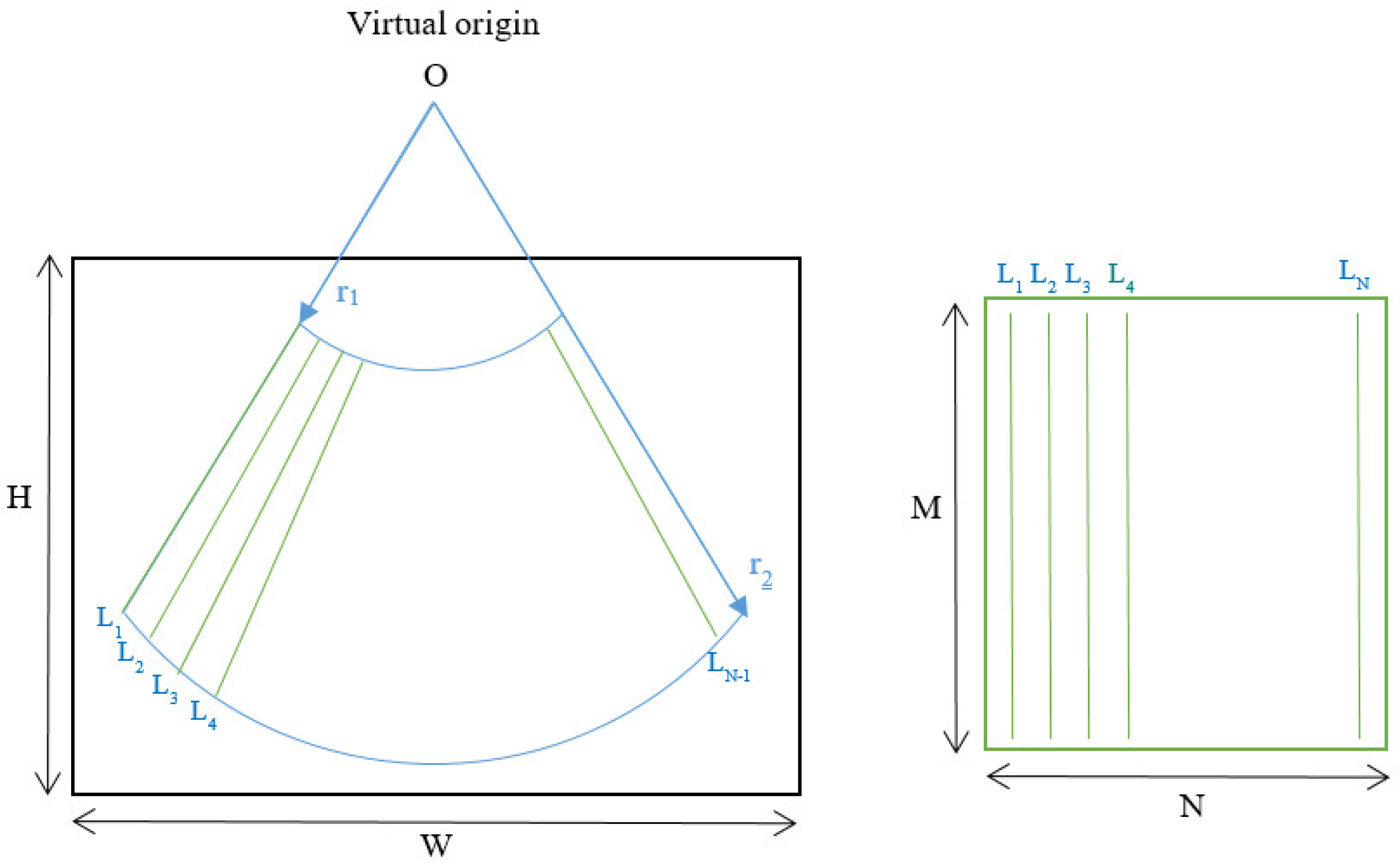
Figure 3. Comparison between sectorial image (a) and B-Scan (b).

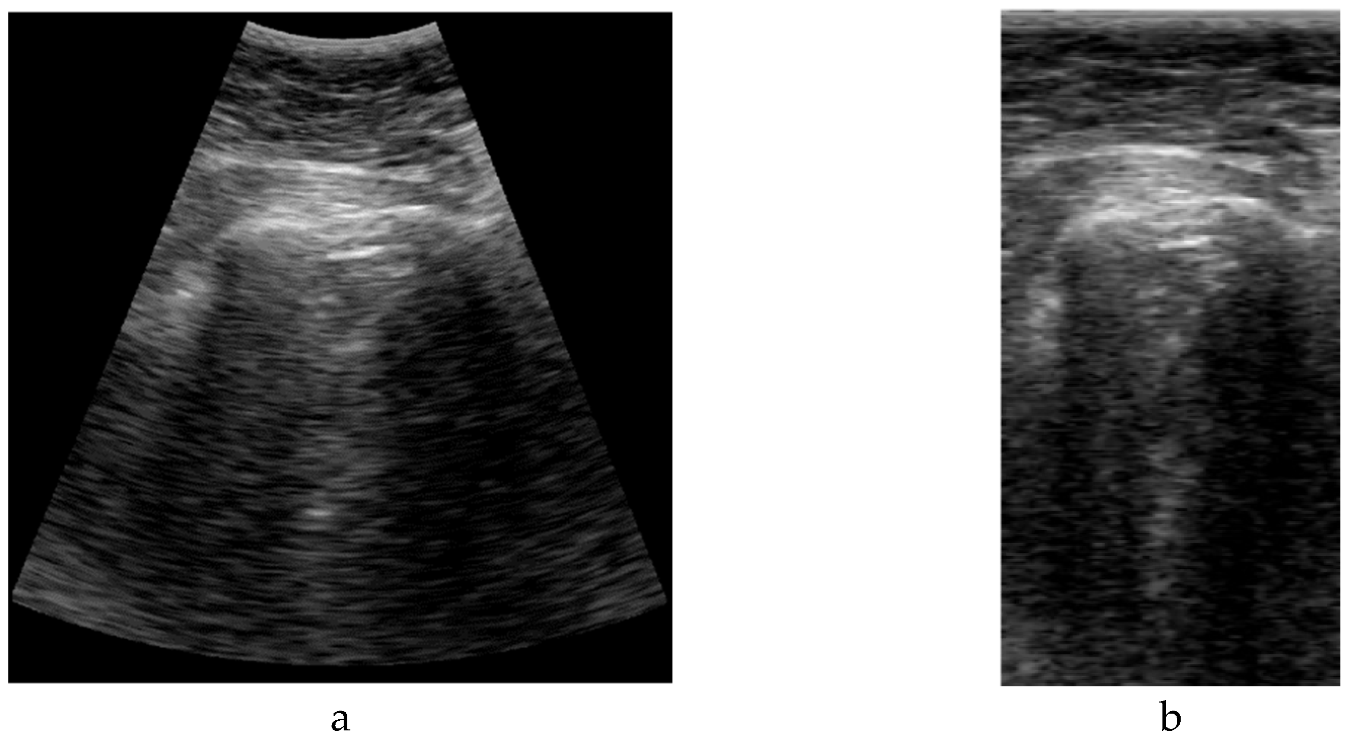
Figure 4. First pleura approximation example. a) original B-scan image; b) filtered image.

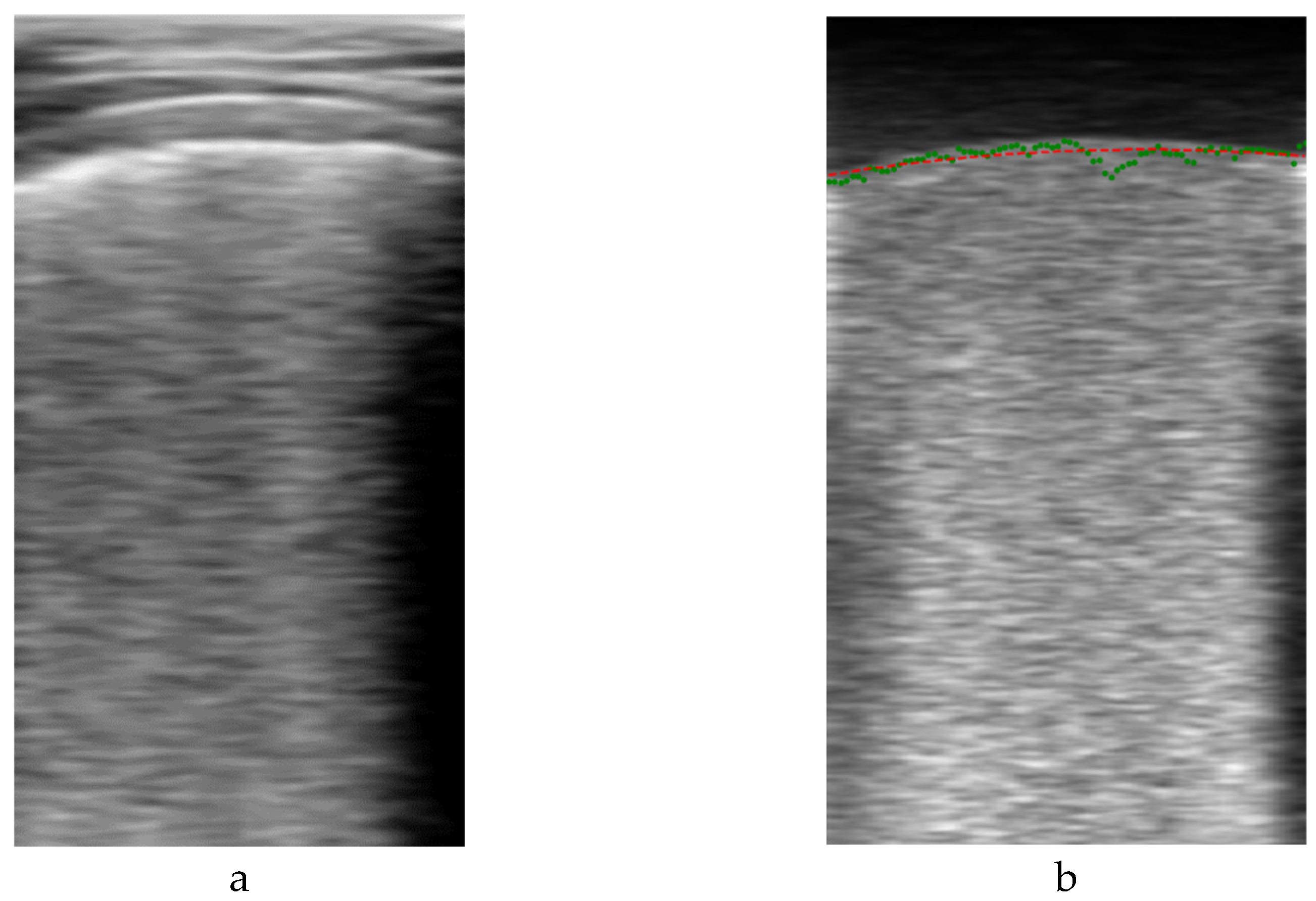
Figure 5. Post-processing adjustment of automatic pleural annotation. a) B-scan image; b) initial pleural annotation approximation; c) final pleura annotation.

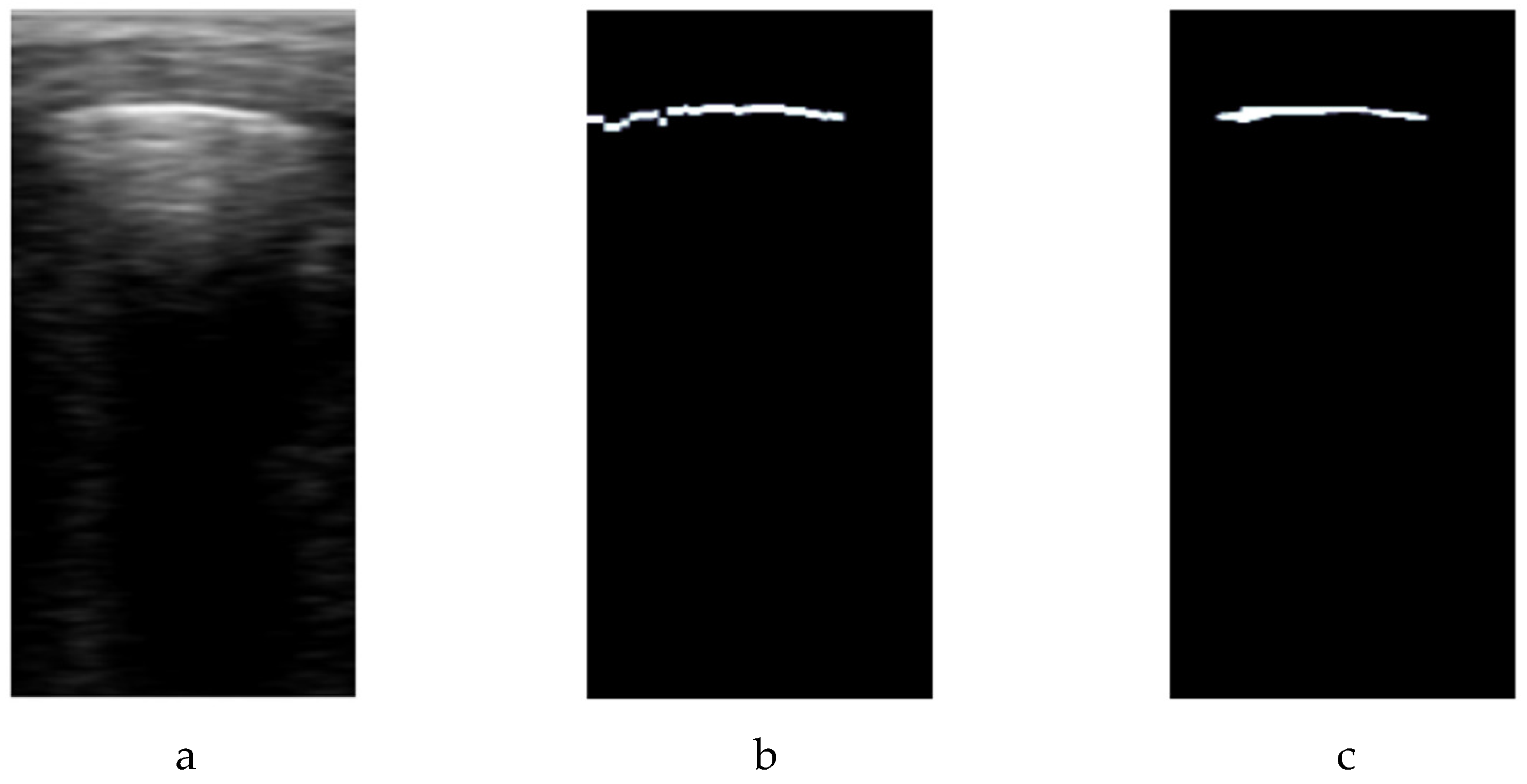
Figure 6. a) Tool developed for consolidation annotation; b) tracking secuence over 4 consecutive frames.

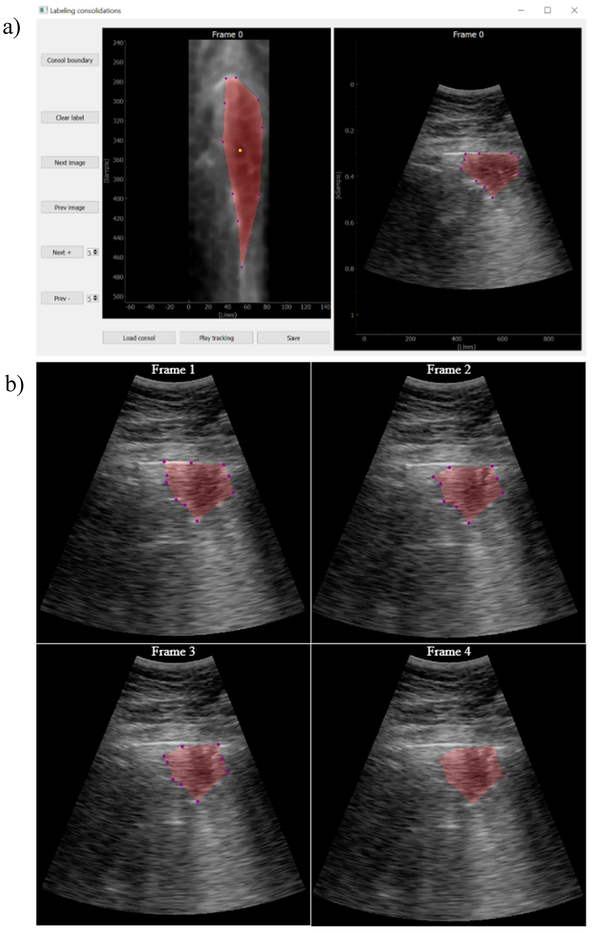
Figure 7. Saturation applied to simulate ultrasound gain variance. a) and b) are the same b-scan applying different image gain and saturating to the scanner full scale value.

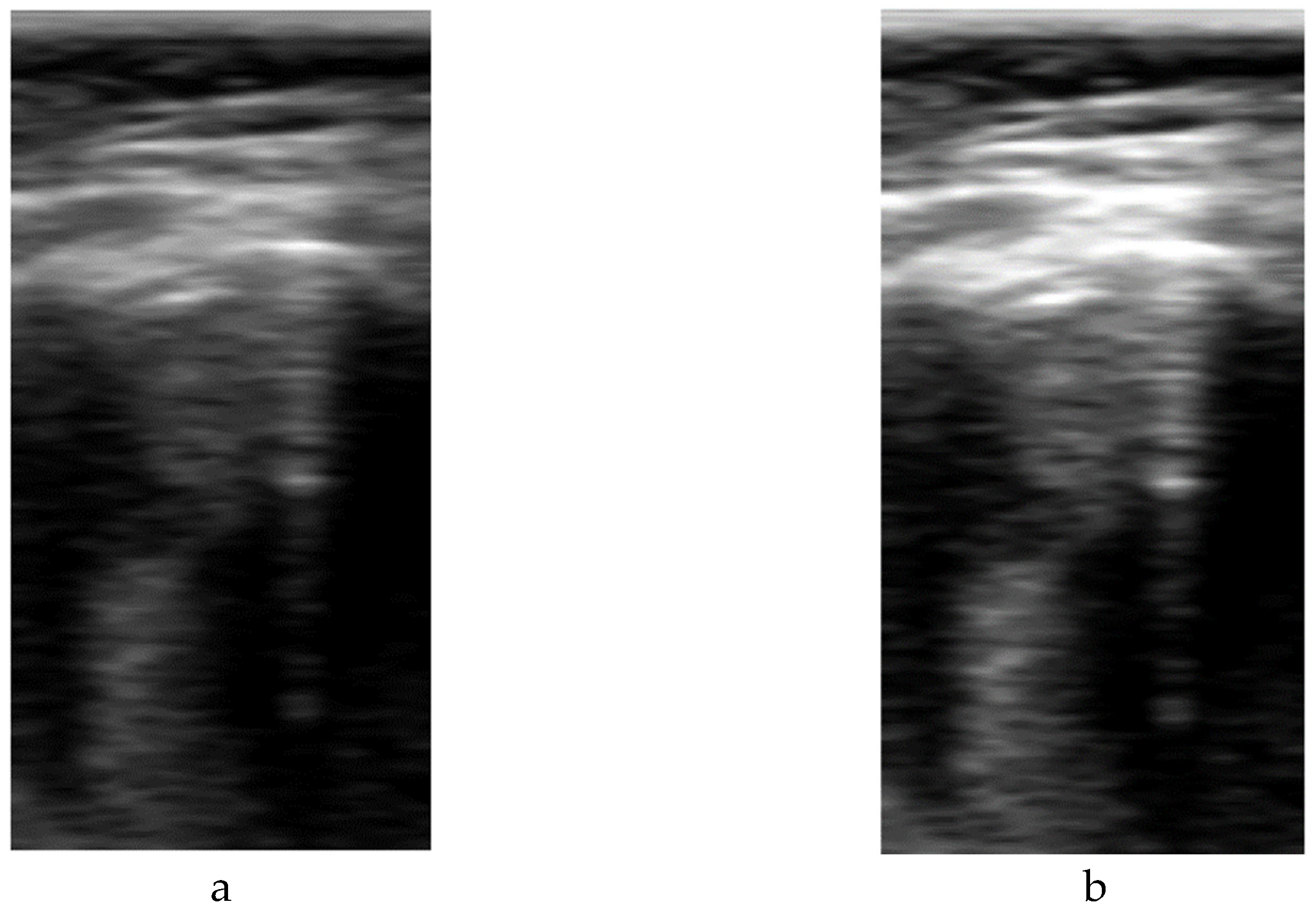
Figure 8. Solution architecture graph.

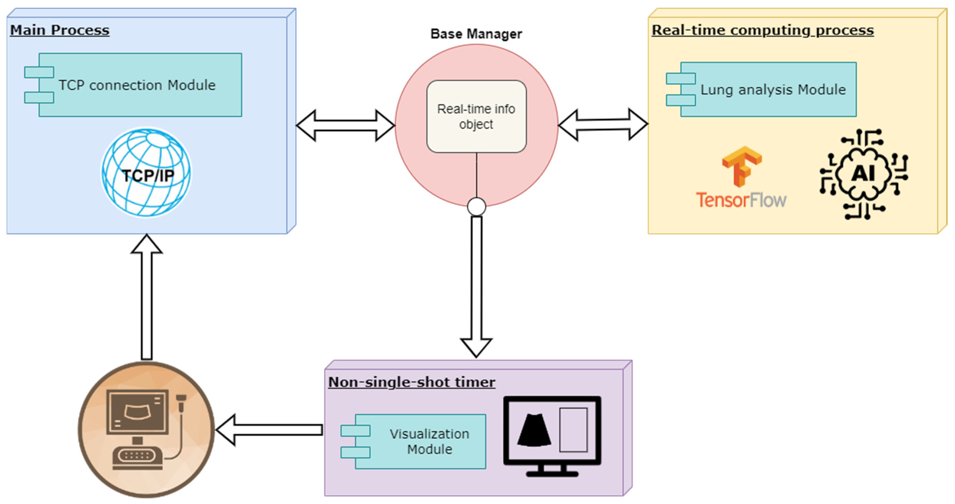
Figure 9. Real-time image processing code flow.

Figure 10. Visualization screen.

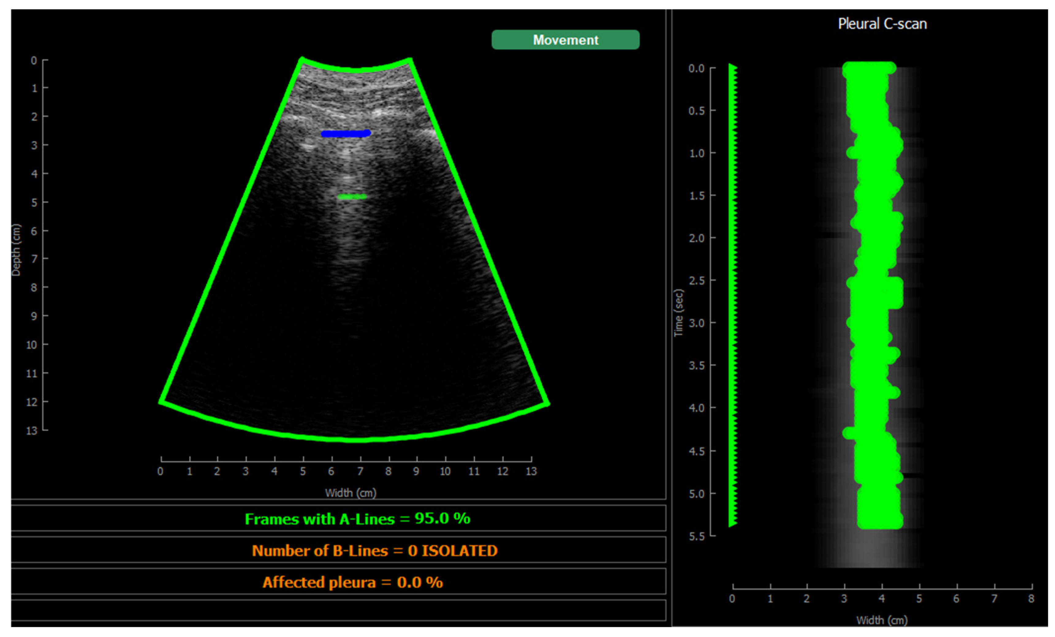
Figure 11. Threshold comparison in CNN output applied for test dataset.

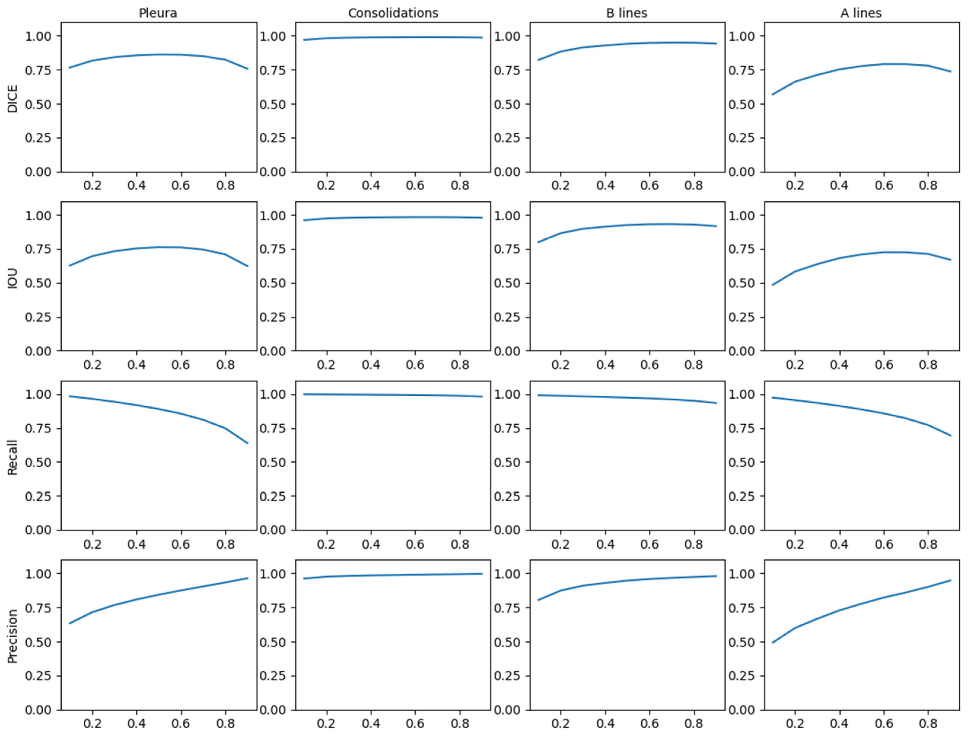
Figure 13. Application visualization sample: a)B-lines (orange) and consolidation (red) detection; b)normal lung with A-lines(green); c) probe movement detected; d) B line (orange) and A-line (green) deteccion on a Lung phantom. On the right of each image the C-scan image is shown.

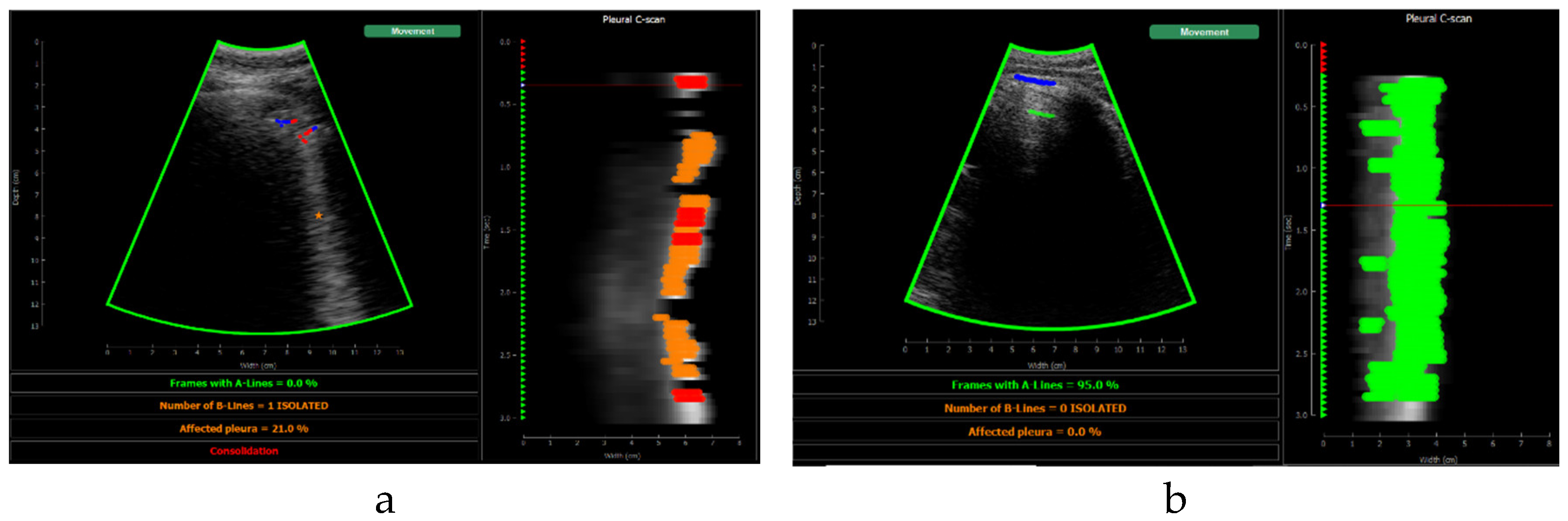
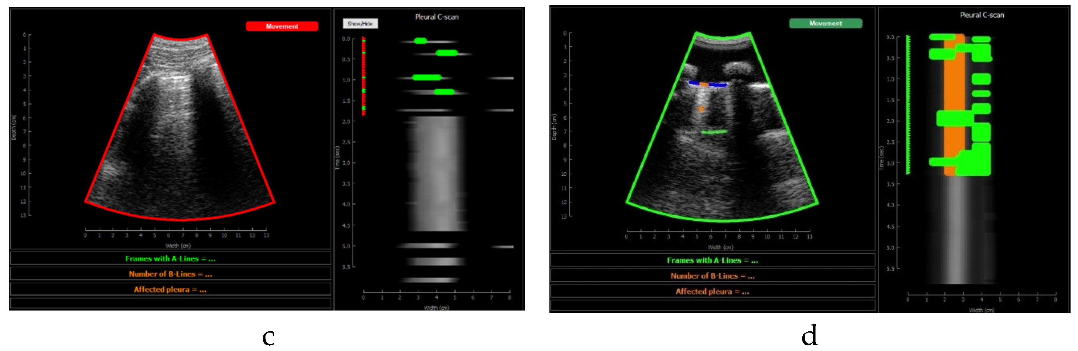
Figure 14. B-line segmentation error examples.

Table 1. Table of statistic metrics of model at a frame level in test dataset.

Metric	Artifact
	Pleura		Consolidation		B-line		A-line
	Mean	Std	Mean	Std	Mean	Std	Mean	Std
Dice coefficient	0.83	0.08	0.96	0.17	0.87	0.30	0.62	0.40
IoU	0.72	0.11	0.95	0.18	0.84	0.30	0.56	0.40
Recall	0.86	0.10	0.97	0.12	0.94	0.17	0.78	0.33
Precision	0.81	0.11	0.97	0.14	0.88	0.28	0.69	0.39

Table 2. Table of statistic metrics of model at a frame level in test dataset.

Artifact	Pleura	Consolidation	B-line	A-line
F1-score	0.83	0.97	0.91	0.73

Table 3. Table of statistic metrics of model at a frame level in out of training patients.

Metric	Artifact
	Pleura		Consolidation		B-line		A-line
	Mean	Std	Mean	Std	Mean	Std	Mean	Std
Dice coefficient	0.77	0.13	0.85	0.34	0.62	0.41	0.48	0.41
IoU	0.64	0.15	0.84	0.35	0.58	0.42	0.42	0.40
Recall	0.78	0.17	0.88	0.31	0.81	0.31	0.59	0.41
Precision	0.79	0.15	0.95	0.20	0.70	0.40	0.64	0.40

Table 4. Table of F1-score of the model at a frame level in out of training patients.

Artifact	Pleura	Consolidation	B-line	A-line
F1-score	0.78	0.91	0.75	0.61

Table 5. Table of accuracy at video level in whole dataset.

	Consolidations	B-lines	A-lines
Accuracy (%)	97.81	88.74	65.79
False positives (%)	0.44	4.09	23.54
False negatives (%)	1.75	7.16	10.67

Table 6. Table of accuracy at video level in whole dataset.

	Consolidations	B-lines	A-lines
Accuracy (%)	89.29	92.86	66.07
False positives (%)	3.57	1.79	26.79
False negatives (%)	7.14	5.36	7.14

Disclaimer/Publisher’s Note: The statements, opinions and data contained in all publications are solely those of the individual author(s) and contributor(s) and not of MDPI and/or the editor(s). MDPI and/or the editor(s) disclaim responsibility for any injury to people or property resulting from any ideas, methods, instructions or products referred to in the content.

© 2024 by the authors. Licensee MDPI, Basel, Switzerland. This article is an open access article distributed under the terms and conditions of the Creative Commons Attribution (CC BY) license (http://creativecommons.org/licenses/by/4.0/).

Copyright: This open access article is published under a Creative Commons CC BY 4.0 license, which permit the free download, distribution, and reuse, provided that the author and preprint are cited in any reuse.

Downloads

Views

Comments

Subscription

Notify me about updates to this article or when a peer-reviewed version is published.

MDPI Initiatives

Important Links

Choose an area of interest and we will send you notifications of new preprints at your preferred frequency.

Disclaimer

Deep Learning-Based Algorithms for Real-Time Lung Ultrasound Assisted Diagnosis

Abstract

Keywords:

Subject:

1. Introduction

2. Methods

2.1. Neural Network Architecture

2.2. Dataset

2.3. Neural Network Input Data

2.4. Neural Network Output Data

2.4.1. Labelling Tools

2.4.1.1. Pleural Line Labelling

2.4.1.2. A-Line Labelling

2.4.1.3. B-Lines Labelling

2.4.1.4. Consolidation Labelling

2.4.2. CNN Output

2.5. Training

2.6. Validation

2.7. Implementation of the Solution

2.8. Main Process

2.9. Real-Time Computing Process

2.9.1. Pre-Processing Block

2.9.2. Model Prediction

2.9.3. Post-Processing Block

2.10. Communication Between Processes

2.11. Visualization

3. Results

3.1. Model Results

3.2. Real-Time Implementation Results

4. Discussion

5. Conclusions

Acknowledgments

References

MDPI Initiatives

Important Links

Subscribe