
Submitted:
18 November 2024
Posted:
19 November 2024
You are already at the latest version
Abstract
Month-long and seasonally persistent apparent tilts in atmospheric radar scatterers have been measured with a network of 6 windprofiler radars over a periods of two and more years. The method used employs cross-correlations between vertical winds and horizontal winds measured with the radars. It is shown that large-scale apparent tilts which persisted for many weeks and months were not uncommon at many sites, with typical tilts varying from horizontal to 2o from horizontal. The azimuthal and zenithal alignment of the tilts depend on local orography as well as local seasonal atmospheric conditions. It is demonstrated that these apparent tilts are not true large-scale phenomena, but rather are a manifestation of coordinated motions within turbulent radar-scattering structures at scales of a few metres and tens of metres, with these structures themselves being defined by larger-scale and longer-term physical processes. Implications for interpretation of the nature of turbulent eddies, the accuracy of vertical wind measurements, and the nature of layering and scattering in the real atmosphere, are discussed. For the first time, a method which allows accurate measurement of the mean off-horizontal alignment of anisotropic turbulent eddies is introduced.
Keywords:
radar
; turbulence
; radar-scatter
; reflection
; atmosphere
; refractive-index
1. Introduction
From as early as the 1970’s, atmospheric radar scattering from well-defined layers of refractivity-index in the atmosphere have been observed by wind-profiler radars, (e.g., [1,2,3,4,5,6,7,8,9,10,11,12,13]. More recently such observations have been further summarized by [14] (among others). Full explanation of these results is still incomplete, since the scattering demonstrates some peculiar characteristics, including strong aspect-sensitivity. Interestingly, different models even propose seemingly opposite viewpoints, from highly stable regions to extremely turbulent regimes.
Figure 1 shows some sketches of some representative models which have been presented in the literature, in order to give some idea of the variation of explanations.
Figure 1(a) shows entrainment, in which sheets are drawn horizontally into each other and form alternating layers of refractivity e.g., [10]; this model requires quite still air and little to no turbulence. Refractive-index edges between adjacent layers must be quite sharp, being completed in less than half a radar-wavelength (i.e., < 2-3 m thick). In contrast, Figure 1(b) shows extreme turbulence with sharp edges, as proposed by [15]; this model is now generally considered as unrealistic, but has been retained here for historical reasons. Figure 1(c) shows the possibility of small-scale waves called “viscosity” waves, aligned quasi-horizontally, with a vertical wavelength equal to half the radar wavelength, acting as radio-wave reflectors [16,17]. These require non-turbulent conditions. Figure 1(d)-(f) show more sophisticated turbulence models than Figure 1(b). In particular, they simulate radio-scattering eddies as ellipsoids, with eddies at the edges of the layer having the largest axial-ratios. Elongated horizontal structures with rapid height-varying vertical refractive index can also exist at the edges, as illustrated by undulating horizontal broken lines (e.g., [18] and references there-in). Both the eddies and the striated structures can back-reflect radio waves, although experimental evidence for such structures is less clear. Figure 1(d) shows the case that the eddies are aligned with the edges of the layer, while Figure 1(e) shows the possibility that the eddies are aligned at an angle to the layer. Figure 1(f) shows the case that the eddies are aligned quasi-randomly. Figure 1(e)-(f) are considered more appropriate for turbulent scatter than Figure 1(b). In Figure 1(a) and 1(c), the radar signal returned to the ground is considered to behave like reflection of light from a rough mirror. In cases 1(e)-(f), the process is not considered to be reflection, but rather a “scattering” process (e.g., [3,19]). For radar signals incident perpendicular to the long-axis of the ellipse, strong signal is scattered perpendicular to the long axis of the ellipse, but signal is also scattered at angles which are not perpendicular, albeit with diminishing energy as one moves further from the perpendicular axis. Only ellipsoids with a width of order of one half of the radar wavelength produce significant scatter; other ellipsoids at other scales exist but are not drawn. More details on the relation between the so-called “scatter polar diagram” and the axial ratio of the ellipsoids can be found in [20], Figure 7.18. The radar responds to these eddies - if the layer and the eddies have different orientations, then the scattering eddies will be the main defining feature, unless other quasi-horizontal extended strata (like the broken undulating lines) also co-exist nearby.
Such layers have also been seen by other methods. [21] have observed similar structures by optical methods in clouds, and these have thicknesses of ~7–30m with relatively sharp edges. In-situ observations using kites, radiosondes, high-altitude balloons, helicopters, drones and other instruments also reveal similar structures e.g., [7,8,9,10,14,18,22] among others.
However, most studies have been relatively short-term, covering a few hours or perhaps a few days. Our purpose in this paper will be to make studies over much longer time-scales - monthly, seasonal and over multiple years. The above shorter-term discussions will nevertheless prove important in interpretation of our results.
As a final point in this introduction, it is of value to determine typical isobaric slopes that might be expected in “normal” atmospheres. We will determine typical slopes of isobars in various circumstances. Recognizing that the pressure in an isothermal atmosphere is given by P=P0 exp{-z/H}, where H is the scale-height, then dP = P0/H exp{-z/H}dz, so δz = H/P0 exp{z/H}δP. Hence at ground level, for H≈8500m, a change in pressure of 1 hPa corresponds to approximately 8.5 metres in height. At 10 km altitude, the temperature is less, so the scale-height is 6.5 km, but the exp{z/H} term needs to be included, so 1 hPa corresponds to ~30m of height.
As an example, if a low-pressure system is at 980 hPa and a high-pressure system is at 1020 hPa and these are separated by 500km, the mean slope between systems is tan−1{(1020-980)×8.5/500e3} = 0.04o. If we consider a frontal system, and suppose that the change in pressure is 20 hPa across a distance of 50 km, the mean slope is 0.2o. At 10 km in height, 1 hPa corresponds to a 30m displacement in height, so these angles will be ~30/8.5 times higher, so up to 0.6o in an extreme frontal system.
Another useful example comes in the form of sea- and lake-breezes. [23] estimates a pressure gradient of 1 hPa per 50 km as typical of a sea breeze, so that would give a slope of ~ 0.01o. A more extreme, but nevertheless realistic, case would be a situation in which the change in pressure might typically be 4 hpa across a horizontal traverse of 50 km, giving an isobaric slope of tan−1( 4.0*8.5/50e3) = 0.04o. At the top of a sea-breeze circulation, (say at 4 km altitude, where the temperature is ~270K, so that H~ 7.6 km, and exp {z/H} = exp(4000/7600) ≈1.7), then the pressure changes by 1 hPa across ~13m in height, so the angle of an isobar could be ~ 13/8.5 times more, or ~0.06o.
These values will prove useful later as limits for our data. We will measure monthly averages of the slopes so it is probably fair to say that slopes of more than 0.2o might be considered unrealistic if they were to be explained as simply slanted isobars. Slopes larger than 0.5 degrees would definitely need alternate explanations.
2. Methodology
Testing of short-term behaviour of atmospheric layers by radar methods usually involves beam steering methods, spatial interferometry, or spatial correlation techniques using multiple antennas (e.g., see [24,25,26], among others: [20], chapter 9 contains more details). These procedures are well-suited for studies on scales of hours to a few days. However for this current, longer time-scale, study we adopt a different technique. Correlations between horizontal winds and vertical winds were used. Studies were performed on time-scales of one month, for each month of the year at multiple sites; hourly averages of both horizontal and vertical winds were used. Horizontal winds were calculated using radial velocities determined with 4 off-vertical beams, and vertical winds were calculated using radial velocities on a nominally vertical beam. Using four off-vertical beams for the horizontal wind determinations helps null out the impact of potential effects of biases in zenithal pointing directions (see the next section). Correlations between the hourly vertical wind and the horizontal wind component were determined for all azimuthal directions from 0 to 360°, and then the direction associated with the largest statistically significant correlation coefficient determines the azimuthal direction of any layer tilt which might be present. Once the optimum azimuthal direction has been found, the zenithal layer tilt is found by calculating a least-squares fit between the vertical winds and the horizontal wind components along the azimuthal direction of layer-tilt. Early attempts at this procedure were presented by [27]), but this new study substantially expands the scope of that work.
3. Instrumentation
3.1. Radar Details
Data from six radars in Canada were used. Five of these formed part of the O-QNet, a network of windprofilers in Ontario and Quebec in Canada. O-QNet radars that were used were Walsingham, Harrow, Negro Creek, Wilberforce, and Montreal (McGill Macdonald campus). Walsingham and Harrow are located near the northern shores of Lake Erie, and Negro Creek is located slightly east of Lake Huron. The McGill radar is located at the junction of the Ottawa river and the St.Lawrence waterway. Maps of the sites can be found in [28], Figure 1 or in [29], Figure 1. The sixth site was an arctic site at Eureka, Canada (80oN, 86oW) and has a complicated geography, being mountainous as well as being located close to several fjords and sea-inlets.
All radars operated at frequencies between 40 and 55 MHz, and had peak pulse powers of 32-40 kW. Radar configurations and specifics can be found in [30], especially Figure 1 and Table 1 and Table 2. For the purposes of this paper, the main points are that (i) 2-way-half-power-beam-widths were typically1.6o to 1.9o, with the exception of Negro Creek, which had a value of 2.3o, and (ii) pulse-length resolutions were 500m above 2.6 km altitude, and 250m below. Duty cycles were typically 5%, and the antenna-array one-way gain was ~25 dB. Off-vertical beams were generally 10.9o off-vertical.
Data analysis of the raw data followed the procedure outlined in [31] for the CLOVAR radar. This includes some extra features not normally applied on other radars, but which were applied for all radars used in this study. In particular, data-lengths of ~30 to 35 secs were recorded on each beam, and extensive Fourier and spectral analyses were applied. In particular, Figures 5, 6, and 7 of that paper demonstrate the methods used in real time to recognize and remove spurious signal. Removal of ground-echoes and low-frequency oscillations is demonstrated in Figure 7 of [31]. This capability is unique to the O-QNet radars, and of particular value to our experiments for this paper, in which we need to have reliable vertical winds: all ground echo signatures within +/0.03 Hz of zero frequency were automatically notched out, but broader spectra close to 0 Hz could still be retained to some degree (with the centre notched out), often with sufficient information to allow some spectral fitting. As a rule, though, radial velocities less than ~0.1 m/s in magnitude (frequency offset of 0.03 Hz) were ignored, or at least treated cautiously.
3.2. The Vertical Beam
A very important aspect of this analysis is the degree to which the main radar beam is truly vertical. Even a perfectly flat antenna array might have unknown tilts due to refractive-index structures below the ground, variations in soil composition, and possibly errors in the length of feeder cables to the antennas. So care is needed here.
Before we begin this discussion, it is emphasized that in regard to array construction, all surveying in regards to height for the O-QNet was done using a laser leveller. Critical measurements were made at night-time, when the laser beams were clearly visible over distances of ~100m. Measurements of the horizontal plane of the array were also taken from multiple, redundant positions. An error of 30 cm in height across the array of width ~80m corresponds to an error of 0.1o, and laser levelling produces an error of less than 2-5 cm over that distance, so from a surveying perspective, our radars are mechanically flat to better than 0.02o. All cable feeder cables were cut to exact multiples of one wavelength (+/- 3 mm), using impedance meters to verify that resonance had been achieved. Accuracy of better than 0.5 cm per cable can be assured. Nevertheless, caution is always required, and so we now discuss other procedures by which the degree of net tilt can be evaluated.
One such test is to consider opposite pairs of tilted beams. A tilt in the vertical beam will also lead to tilts in the off-vertical beams - if the nominally-vertical beam in fact has a tilt of 0.2 degrees (say), this will result in opposite pairs of beams having differing tilts. For example, if the nominal tilt is 10.9o, then these will appear as 11.1o and 10.7o in the tilted scenario. When averaged across both beams, the “horizontal winds” will be quite accurate, as one beam underestimates, and the other overestimates. Nevertheless, in such a case, a detailed comparison of individual measurements on opposing beams will show an offset between the 2 beams. This therefore offers a way to check on the vertical nature of the array.
We therefore checked the vertical nature of the array by comparing radial measurements on oppositely directed off-vertical beams. As an example, Figure 11 from [31] was used. This figure shows radial velocities on nominal east and west beams for the Clovar radar. A regression calculation of radial velocities between beams, taken at similar times (to within 10 mins of each other), shows regression slopes of g0x = 0.9500 +/- 0.054 and g0y = 1.006 +/- 0.058 for regression of the “west” beam on the “east” beam and the converse, respectively. The offsets of the best-fit lines were 1.54 +/- 0.87 and -0.672 +/- 0.953 respectively.
Taking this one step further, and applying the dual regression procedure presented by [32], which is designed for cases in which both variables have errors, shows a most likely regression slope of 0.97 +/- 0.06. This corresponds to a possible tilt of 0.2 +/-0.25 degrees. The possibility that the true tilt is zero is not excluded by these results, but even a tilt of 0.2o will prove acceptable for our studies (as will be established in more detail later). The Clovar radar was the prototype of all of the O-QNet radars, so the tilt angles presented here are representative of all subsequent O-QNet radars. (The Clovar radar was not used in this study because it was a developmental system: it ran from 1994 till 2008, but usually in a mixed mode, alternating between tropospheric modes, mesospheric modes, and meteor-radar modes, so no months were used exclusively for tropospheric studies. It was also low power (6 kW peak compared to 32-40 kW for the O-QNet radar). Further, the Clovar radar was turned off in 2008 due to a large metal building that was built within 10 metres of its edge, drowning the radar signal and contaminating the data. Since the O-QNet radars offered higher power and continuous data, and our data were concentrated on the periods around 2010 to 2012, the Clovar radar was excluded from further contributions to this study. Finally it is worth noting that the above analysis assumes that the “horizontal wind” was indeed truly horizontal: we will return to this point later.
It is therefore concluded that the mechanical alignment of the arrays used in this study were in general better than 0.2o. Further commentary will ensue later in the discussion section.
3.3. Correlation Analysis
The key point in this analysis is that we do not assume that the nominally vertical beam on average receives maximum scatter from directly overhead, but rather allow the direction of received signal to be more general. Denoting the horizontal hourly-averaged wind speed as U, assuming that this wind blew from a direction Ψ clockwise from geographic north, assuming that the direction of maximum scatter received on the vertical beam on average was at a zenithal angle of θ from overhead, and assuming that the maximum scatter on the vertical beam occurred from a direction ϕ0 clockwise from true north, it would be expected that the radar would, on average, record a mean radial velocity on the nominally vertical beam of
where, as usual, a positive value for Wu means motion away from the radar. Angles are considered to be in degrees. If ϕ0 corresponds with the direction toward which the mean wind blows, then ϕ0 = Ψ + 180o, and the cosine term is unity. The directions θ and ϕ0 may be non-zero for a variety of reasons e.g., the scattering entities and layers may not be horizontal (see Figure 1), or the nominally vertical beam might not be truly vertical. These (and other) possibilities will be considered in due course; for the moment it is assumed that θ and ϕ0 may ≠0.
Wu = U sinθ cos(Ψ + 180o − ϕ0)
The radial wind measured by the vertical beam of the radar (as determined from frequency offsets in the raw spectrum determined when the nominally vertical beam is used, (e.g., [31]) will be referred to as the “nominal vertical wind” (w) - this terminology is used in order to recognize that w may not be the true vertical wind, and may suffer biases due to scattering layer tilts and even modest tilts of the radar beam itself. The horizontal winds (U, Ψ) were determined from radial velocity measurements on the 4 off-vertical radar beams, and are assumed to be accurate. The radar-derived horizontal winds have been shown to be accurate by extensive comparisons with the NCEP North American Regional Reanalysis (Taylor et al., 2016). Throughout the analysis, we used hourly averages of w and Wu. Representative wind data-rates are seen in [33]. Hourly data were generally available continuously from ~400m to ~7 km altitude, with 90% acceptance from 7 to 9 km, and ~70% acceptance from 9 to 11 km. Data above 11 km were available ~50% of the time up to ~14 km altitude.
Next, a value for θ was chosen, and systematically varied ϕ0 from 0 to 350o in steps of 10o. We will refer to this initial guess of θ as θi. Normally a value of θi = 1o was chosen, but other choices may be selected at times. When using θi, Wu is referred to as Wui. For each new ϕ0, Wui was determined for every hour of the month, and then the Pearson cross-correlation coefficient between the measured hourly “vertical wind” (w) and Wui was determined for each recorded altitude. The primary purpose was to find the value of ϕ0 for which the Pearson coefficient maximized in magnitude. This was done independently at each recorded altitude. The choice of θi does not affect the correlation coefficient, and can be chosen at the discretion of the user. Determination of the true value of θ will be described shortly.
A typical result of this correlation analysis is shown in Figure 2. More detailed discussion will be left to the next section, but the following points are evident. First, high levels of correlation were found, especially above ~6 km. Equally notably, the heights around 3 km showed very weak correlation in this case. It is emphasized that while the cases of high correlation catch the eye, the cases of low correlation are equally important. These do not mean poor or missing data - they indicate cases where the scattering layers were truly horizontal, and the horizontal winds and vertical winds were uncorrelated. In fact to some extent they represent the “ideal” situation. The correlation coefficients are clearly rotationally anti-symmetric, with strong correlations and strong anti-correlations occurring 180o apart (reds and blues). This is expected from Equation (1). Physically, this simply means that by viewing the layers with an azimuthal addition of 180o, the regression slopes of the layers change from positive to negative (or conversely). It is also important to note that in Figure 2 the correlations (both magnitudes and positions of maximum ϕ0) are strongly height-dependent. (Note that within this paper, several uses of the word “slope” exist. The word is used to refer to slopes in the atmosphere associated with layer tilts, but is also used in regard to slopes of regression fitting (as in this paragraph)).
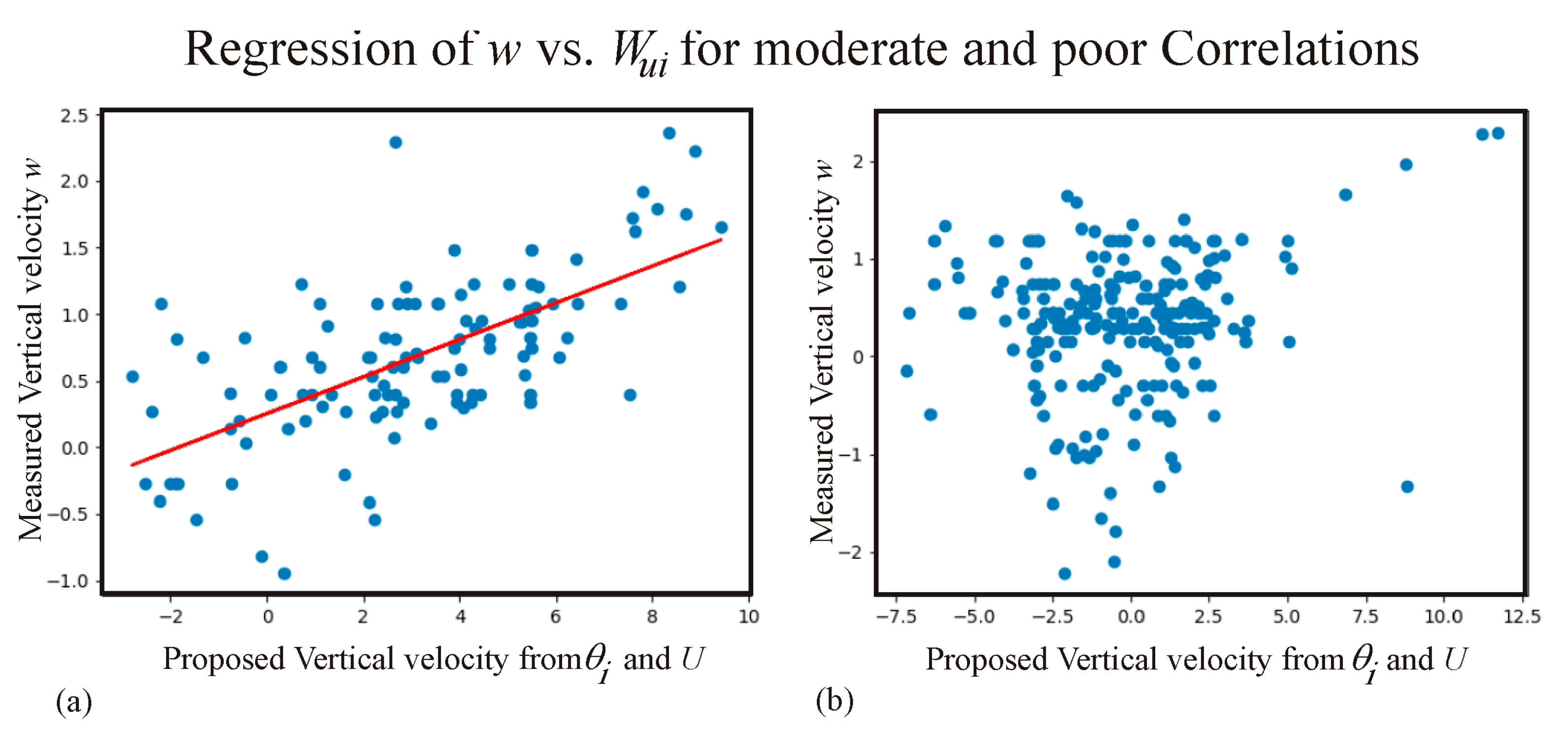
The next step was to find the correct value for θ for each height. To do this, the regression plot of w vs Wui was re-determined, but only for Wui values determined using the value of ϕ0 at the optimum cross-correlation coefficient. A regression plot was also produced, allowing a best fit regression slope to be calculated. Two examples are shown in Figure 3, with Figure 3(a) showing the case of a relatively good correlation, and Figure 3(b) showing a case of poor correlation. In these case, θi was taken to be 10o, in order to produce a better display. For our analyses, θi was usually taken as 1.0o.
Adapting Equation (1) for cases where the θi is user-defined, we write
where we have added the best-fit regression slope as si. In general si will not be unity, since θi was user-defined (for purposes of doing the cross-correlation). If the true angle sought is denoted as θ, then there is no need for a “regression slope” term, since the condition we seek is w = Wu , or a “slope” of unity. In this case
w = si Wui = si U sinθi cos(Ψ + 180o − ϕ0)
w = U sinθ cos(Ψ + 180o − ϕ0).
Comparing Eqs (2a) and (2b), it is seen that sinθ = si sinθi. Thus once the best fit line has been produced for our chosen θi, the value for θ (which is the tilt-angle we seek) can be deduced through the relation
or for small angles,
sin(θ ) = (measured slope deduced using θi ) × sin(θi).
θ ≈ (measured slope deduced using θi ) × θi
Figure 3.
Regression plots of measured vertical velocities w vs. simultaneous estimates of Wui (from Equation (1), with θ set to θi ). In these cases, θi is taken to be 10o, in order to produce a better display. Case (a) uses an azimuthal angle ϕ0 of 50o, at a altitude of 5.5 km, and is chosen at the point of largest correlation coefficient ρ for this height (in this case ρ =0.4). Case (b) applies to an altitude of 7.5 km, and was chosen as a representative case when the correlation coefficient was close to zero: this occurred at a value for ϕ0 of 5o.
In this last equation, the angles may be in either radians or degrees—if we choose θi = 1o, then the ideal angle θ is just equal to the “regression slope of best fit for θi = 1”, expressed in degrees. Note that here we use two separate applications of the word “slope”, which we distinguish as “regression slope” and “tilt slopes”. When we use θi = 1, the “regression slope” and the geophysical tilt-slopes of the atmospheric layers become numerically equal, but this only occurs if θi = 1. However, the regression slope and the geophysical (tilt) slope are conceptually very different. If we use a different value for θi (e.g., 2o), then the regression slope needs to be converted to the tilt-slope by either Equation (3a) or (3b).
Before proceeding to look at results, it is worth commenting on the rotational anti-symmetry demonstrated in Figure 2. In that figure, it was noted that the red and blue sections were antisymmetric. Red (positive correlations) correspond to cases in which, along the direction ϕ0 , the vertical velocity increases as the mean horizontal wind component along the direction ϕ0 increases. Blue (negative correlations) mean that along the direction ϕ0 , the vertical velocity increases as the mean horizontal wind component along the direction ϕ0 decreases. Each provides the same information in a slightly different way. We choose to accept the red cases (positive correlation), though the blue cases carry the same information, albeit in a slightly different way. For purposes of interpretation, there may be reason at times alternate between the two descriptions, but for purposes of this section, we will retain only the positive correlations and their associated ϕ0 values.
4. Results
4.1. Correlations
The value of ϕ0 at which the correlation coefficient maximizes is called ϕΜ (M means max value of ρ). ϕΜ varies as a function of month and height. The value of ϕΜ at each height and for each month was subsequently found, and we then recorded the value of ϕΜ , the value of the correlation coefficient in that direction (ρM), and the regression-slope of the best-fit line (sB). The value sB was then used to determine θ, as described above. The optimum value of θ will be referred to as θB, where B stands for “Best” fit (see Figure 3(a) as an example). The offset of the least-squares fit (demonstrated in Figure 3) at Wu=0 was also recorded. The layer-tilt (also called the layer-slope) is usually expressed in degrees, and represents the tilt of a layer from horizontal. Graphs of these 3 parameters were then produced: examples are shown in Figure 4.
While the different months are colour-coded, the main purpose of the graphs is to show typical values, variability and spreads in values. Of particular note are the facts that (a) the correlations were generally > 0.2, with only 50 points out of 325 (15%) having correlations < 0.2 (and only 20 out of 325 (6%) having a correlation < 0.15), (b) the azimuthal directions were not random, but were mainly limited to a range between approximately 10o and 100o for Harrow in 2010, and (c) the layer-slopes (tilts) were generally between 0.4o and 3o in this case.
Again, it is emphasized that a correlation coefficient of around zero does not mean in any sense “bad data” - indeed the cases with ρM = 0 actually represent the “ideal” cases when the layers were close to horizontal. As seen, this seems true on only ~20% of occasions. The other 80% correspond to situations with non-horizontal layering. Reasons will be discussed further in the “Discussion” section.
Of significant note is the fact that tilts as high as 2.5o and even 3o occur. These are much larger than the estimates demonstrated at the end of the “Introduction”, so it is clear that the simple idea that these tilts are due to large-scale tilts in the isobars is not at all appropriate. For now we concentrate on the measurements: explanation of the reasons for the tilts will be left to the “Discussion” section, although we will hint here that Figure 1 will be key to these discussions.
For analysis purposes, the raw data shown in Figure 4 are not ideal, and some averaging is needed before any trends stand out. Different averaging schemes were tested, including “height-averaging” and cross-month averaging. In the end, the best scheme for interpretation proved to be a 3-point running mean vertically and a simultaneous 3-point running mean over successive months. In cases where there are missing months, forbidding calculation of running means across successive months, a 5-point running mean with height is used, as it gives reasonable smoothing but retains sufficient height-structure. Three-point running means with monthly averages mean that only the data at 3-month steps are truly independent, so the results can best be considered as “seasonal” results.
A sample plot of the correlation coefficients smoothed with this 3×3-point running average is shown in Figure 5 for the Negro Creek Site. This figure shows that with the 3×3 running average, the graph appears less noisy, and trends like the increasing mean correlation as a function of height are now clearly visible. In this case, months range only from February to November, since, for example, “February” is an average over January, February and March. Hence an average for January is not possible without also using December, 2009. Likewise December 2010 is missing.
In later discussions we will in fact create running means which cross over successive years, but this is not necessary for the purpose of this illustration. This graph is quite representative of all sites, with the average values of ρM increasing with height, and typical largest correlations reaching ~0.4-0.6.
No further analysis of the correlation coefficients will be presented - the primary purpose of their calculation was to identify layering alignment (when layers existed) and so allow determination of ϕΜ , and thence θB. The primary focus will be on the tilt angle θB.
Because the procedures and results presented here-in are quite new, we chose to be very cautious in the data quality accepted. Hourly average data required at least 5 horizontal wind measurements per hour at any height, and at least 3 measurements of w per hour at each height. Furthermore, over 90% of the hours in each month had to have acceptable data, so while most radars had data in all months of the year, there were frequent months which were excluded from our particular analyses due to insufficient data. In the main, we used the year of 2009 and 2010, though in some cases data from 2011 and 2012 were available.
4.2. Azimuthal Alignment
Figure 6 shows some representative azimuthal angles ϕΜ. Data in Figure 6 were determined as a “composite year”, taking the year (either 2009 or 2010) with the largest number of available months as the “anchor-year”, and filling in months missing from that year with the corresponding month from the alternate year. It will be noted that for the sites of Negro Creek, Walsingham and Harrow, the azimuthal alignment of the tilted layer was between 30o and 130o, so roughly aligned with the direction of the prevailing winds at these sites. We do not investigate the relation between the tilt alignment and the prevailing wind in detail here, as the main purpose is to establish the existence of these tilted layers. Detailed studies of relations between tilt alignment and prevailing wind directions could be a topic of future study.
Generally, most months at all sites showed consistency between consecutive months. Behaviour is modestly well defined. ANOVA (ANalysis Of VAriance) tests were performed, and showed that all sites behaved independently, and hence were not simply some form of “noise”.
ANOVA tests will be discussed in more detail later.
In regard to Figure 6, apparently anomalous profiles do appear, particularly in April at Eureka and in February at Negro Creek. Unusual events are a natural part of any weather history. In the case of Eureka, no data were available in the preceding or following months (March and May), so sanity checks were not available. It is most likely that there was a sustained event of strong winds from the south for a significant fraction of April in this year, rather than the more common prevailing winds from the west, which may have resulted in re-alignment of the tilted layers for a significant portion of the month.
4.3. Zenithal Tilts
We now turn to study the tilt angles from horizontal. Figure 7 shows 5-point averages of θB over height for the available months of 2010, 2011 and 2012 for Walsingham. No averaging as a function of month were used here: only smoothing with height was used.
Some points are obvious here. First, the winter-time values (black) tend to be smaller, and January and February in both 2010 and 2011 were similar. Second, the largest values are evident in March and May in 2010, in June and July in 2011, and in August and September in 2012. (No summer months were evaluated in 2010). October and November, where available, were generally in the middle. So there is modest evidence of seasonal effects. Hence in order to reduce statistical scatter, some averaging over successive months seemed appropriate.
Therefore in order to present the key results in a modestly compact form, running averages across successive months were employed. Specifically, we used the following process. First, for each site, all years analyzed were used; the number of years were not the same in all cases. Walsingham had data in 2009, 2010, 2011 and 2012. McGill only had data in 2009 and 2010. But all sites had at least 2 years. Then, values of θB were averaged across all years for each month at each site. Some years had missing months, so only available years were used in the averaging. A month of data formed across several years of data in this way is referred to as a “composite month”, and a collection of all such composite months is referred to as a “composite year”. By doing this, most composite years included at least 10 months and in many cases all 12 months were covered. The next step was to create both 3-point and 5-point running means averaged over height. Finally, 3-month running means were created from the 3-point height-based running means for all uninterrupted sequences of composite months. However, for cases where a composite month did not have a neighbour on one or both sides, a running mean across months was not used, but rather the 5-point running means as a function of height were used as a substitute. As an example for a sequence of composite months March, June, July, August, September, and October, with no data in April, May or November, 3-point height averages coupled with monthly 3-point running mean (referred to as a “3×3 running mean”) were used for July, August, and September, while 5-point height-only running means were used for March,
June and October. Use of a 5-point mean was chosen rather than for example a 7-point mean, as 7-point averages and even larger degrade the height resolution too much. Finally, December and January were considered as “sequential”, so that a running mean for January meant averaging over December, January and February, and a running mean for December was formed by averaging over November, December and January.
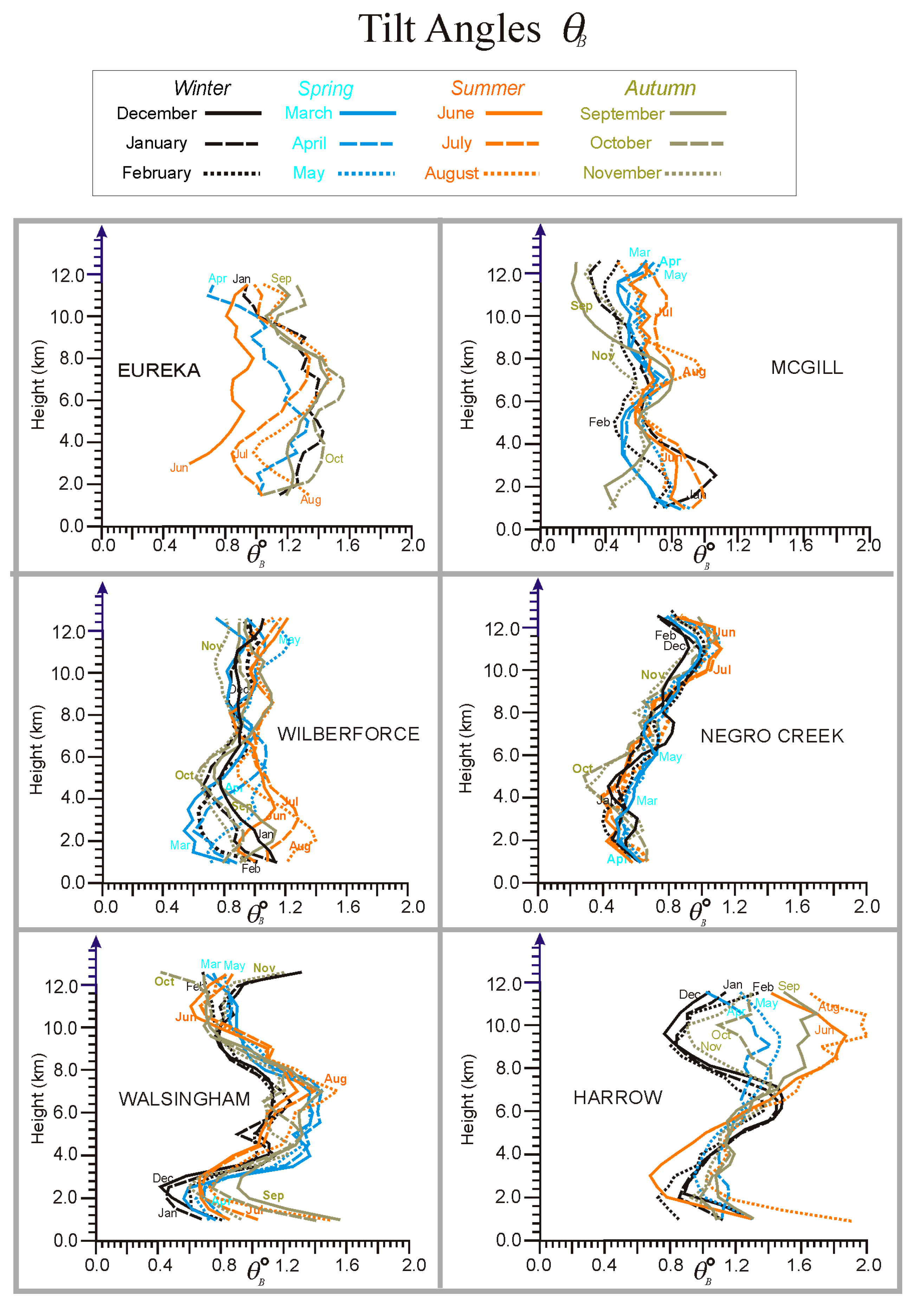
Results of such averaging are shown compactly in Figure 8 for all sites. ANOVA tests verified the independence of each site, as will be discussed later. Behaviours are clearly different at all sites. For example, Negro Creek showed very little seasonal dependence, while Harrow showed a very strong seasonal dependence above 7 km, with smallest values of θB in Winter, moderate values in Spring, then largest values (up to 2o) in Summer and then modest values again in Autumn. On the other hand, Wilberforce showed greatest variability below 4km, again with a clear annual cycle with maxima in Summer. Walsingham showed greatest variability between 4 and 8 km altitude.
Eureka shows June to be distinct from the other months of the year, but it must be noted that this profile came from only 1 month of 1 year, so it is not subject to the same level of averaging as some other months. As discussed earlier, occasional anomalous data should come as no surprise in weather-related studies.
4.4. Statistical Details
Figure 6, Figure 7 and Figure 8 have been presented without error bars, so it makes sense to briefly look at possible errors, especially for the azimuthal angles ϕΜ and the tilts θB. To do this, running 3×3 standard deviations were created. These were formed similarly to the process used to create Figure 6, but for running standard deviations rather than running averages, using mainly 2009 and 2010 data independently. Thus the errors deduced would be upper limits as they involve less smoothing than say the procedures used for Figure 8. Mean standard deviations of ϕΜ over the 2 years were the calculated and results were as follows: Eureka 22.2o; McGill 24.2o; Wilberforce 22.9o; Negro Creek 29.8o; Walsingham 33.6o and Harrow 27.6o. These numbers include any natural geophysical variability, so are larger than random errors alone. These are standard deviations for a single month and height. Using the Central Limit Theorem, and recognizing the smoothing applied in producing the profiles, the standard errors for the mean of any profile will be given by the errors shown above (~20o-30o) divided by √24 (24 points in a profile) or ~5× smaller. Typical errors for the mean were therefore about 5o-6o for each profile, so that individual profiles which differ consistently across all heights by more than ~5-6o are statistically significant. A more thorough treatment using ANOVA’s will be discussed shortly. Greater detail is given in [34]).
In regard to tilts, a similar treatment gives standard deviations as follows: Eureka 0.17o; McGill 0.15o; Wilberforce 0.12o; Negro Creek 0.11o; Walsingham 0.22o and Harrow 0.19o. As above, standard errors for full individual monthly profiles in Figure 8 were ~5× smaller, so ~0.04o. Hence in Figure 8, the differences between Spring and Summer below 5km altitude at Wilberforce, the differences between Spring and Summer at 3-9 km at Walsingham, and the seasonal cycle at Harrow above 7 km all have high geophysical significance. In contrast, the differences between the different composite months at Negro Creek in Figure 8 are likely not significant. Indeed, Negro Creek gives a good opportunity to obtain a visual estimate of the errors. At 8 km altitude, where variability between profiles is least (and hence is least likely to be affected by geophysical variability) the values of θB range from 0.7 to 0.85 i.e.,+/- 0.075. There are 12 profiles, so the error for the mean is 0.075/√(12), or 0.02o. Although only a visual estimate, this is not too different from our estimate of 0.04o above: thus a non-geophysical error for the mean in any profile of ~0.04o is reasonable. Additional fluctuations due to geophysical effects occur on top of this. Overall, unquestionably these tilts are real, and not some sort of noise artefact.
We now turn to ANOVA studies, which involves the F-factor. The F value calculates the ratio of (i) the variance obtained with all the data being treated as one large block, irrespective of classification (group) vs. (ii) the mean of the variances of each of the groups. Colloquially, in medicine, F is often referred to as MST/MSE, where MST is the mean square of treatments, and MSE is the mean square of error. The term “Treatments” does not apply in the atmospheric case, but an ANOVA may be applied equally well here, as is now outlined.
The fundamental idea is as follows. First the user defines what a “group” constitutes. In our case, a sensible choice is to regard every site as a different group. Then the variance of each group is calculated, and these are averaged. The mean value for each site is removed of course during the determination of each variance. Then we consider all the data as one giant collective, and calculate its variance. The larger data-set incorporates all of the means of the separate sites, so if the means at each site differ, this will increase the total combined variance relative to the typical individual variance for the separate sites. Hence if the means all differ, the variance found using all the data will exceed the typical variance for any individual site. So the ANOVA essentially tests the null hypothesis that all means at all sites are equal. If all are equal, it might be true that the “tilts” and “azimuths” determined were due to some common aspect of the radar design or analysis technique, and so might not be geophysical. This will be revealed by values of F around unity. If, on the other hand, the mean values at each site are different, then F will be much larger than unity, and will indicate that the sites are geophysically different. The P-value gives the probability that the data at all sites were due to a process in which all means are equal (e.g., noise, or some radar-related quirk). Determination of the value of P requires two additional input parameters, namely the number of degrees of freedom (generally the total number of points minus 2) and the rejection level. The rejection level is a fraction, referred to as α. Typically α is chosen to be .05, or 0.01 (5% or 1%), and an associated Fα is determined. If the measured value of F exceeds Fα, the null hypothesis is rejected and we say the means differ from equality. This contrasts to a t-test, in which 2 means are compared. In an ANOVA we can only say that either (i) the means at all sites were equal (small F) or (ii) the means differ. In the latter case, it is possible that some means are the same and others differ, or they may all differ - the ANOVA does not single out individual cases.
A Python program was used for our calculations, specifically Python version 3.7 using scipy:stats.f-oneway. In this program-suite, a value for α is not assumed, but rather the program calculates the values of α that corresponds to our value of F, and calls it “P”. So P is a substitute for α. In our case, there were many points, and the number of degrees of freedom well exceeds 100 - at such large values, the relation between F and α becomes largely independent of the number of degrees of freedom.
First, an ANOVA was performed on all the tilt-angles for all the 6 sites separately for 2009, and then again for 2010. For 2009, F = 66.24 and P = 6.33 ×10−60, while for 2010, F = 63.03 and P = 1.41×10−60. So the probability that the data at all sites all originated from the same underlying data-set was exceedingly small, strongly supporting the proposal that the tilts were truly geophysical in origin.
As a second test, since Walsingham was the only site that had 4 years of data, these data were also treated with an ANOVA analysis. The four groups were considered as the four separate years. The goal of this procedure was to investigate if the data from different years were broadly similar. We would expect some year-to-year differences, but some generally similar behaviour (see Figure 7). The results were F = 3.45 with a P-value of 0.019, or approximately 2%. More thorough treatments are presented in [34], but a P-value of 2% is reasonable - it suggests some level of similarity between the different years, but not exact agreement, which is consistent with natural year-to-year variability.
5. Discussion
Various other trends are evident in Figs 6-8: these will not be fully discussed here, and will be the foci of later studies. The key points in this paper are (i) non-horizontal tilt-measurements are real, (ii) there are clear site-to-site differences as verified by ANOVA tests and (iii) these tilts are too steep to be explained by simple isobaric slopes. A primary remaining objective is to explain the origin of these tilts.
Before proceeding with the discussion of mechanisms, it is worth once more reflecting on the nature of the vertical beam. If the beam were indeed tilted off-vertical, then one can imagine specific scenarios in which the layer forms perpendicular to the beam, so the layer appears horizontal as far as the radar is concerned. However, one can also envisage many more scenarios where the effects of the beam-point-direction and the layer makes the effective beam calculated worse. Since the latter is more common, it would be reasonable to assume that over long-term averages, the combined effect of the layers and the beam will generally be additive. Hence the tilts shown in Figure 7 and Figure 8 should all exceed the actual vertical-beam tilt. Therefore the lowest values seen in Figure 7 and 8 would be upper limits on the tilt of the vertical beam. Occurrences of a tilt of 0.2o are moderately common in Figure 7 and Figure 8, tilts of 0.2o to 0.4o are very common. Hence we may conclude that all vertical beams have tilts of less than 0.4o and very likely less than 0.2o. Other studies of azimuthal tilt angles relative to particular radar orientation features were also undertaken in [34], which also further demonstrated that tilts of the main beam were of little consequence in our studies, so henceforth we assume that all tilts measured were geophysical in origin.
In addition, it is important to recall (again) that values of the maximum correlation coefficient ρM of less than 0.15 occurred for layers which were close to horizontal, and in many ways, such occasions apply to the ideal situation of a perfectly horizontal layer - but the fact remains that such “ideal” situations are less common than might be naively expected. We will argue shortly that this expectation of “flatness” may itself be premature.
Next, possible geophysical causes of these tilts need to be considered. Several points need to be noted. First, gravity waves have polarization relations between the horizontal and vertical components of the wave (e.g., [20] and [35] Equation 11.18), so that horizontal and vertical wind components are in phase or in anti-phase. However, this effect is an additional effect on top of the mean wind; our studies have been looking at correlations between the vertical velocities and the total mean horizontal winds, which is not the same. Furthermore while the vertical and horizontal winds are well understood if they are measured at the same point in space, the radar measures horizontal winds using the off-vertical beams, and the vertical wind on the vertical beam, and each are measured at different times and different points in space. Therefore any phase relationship depends on the wavelength and period of the wave. Further, the ratio of vertical to horizontal velocity components becomes smaller as the period increases, and we use hourly averages, which is quite long for a gravity wave. In addition, there may be many waves present at any one time, with different wavelengths and periods. So all in all, the effect of polarization relations of gravity waves will be washed out.
There is one type of gravity wave which might play a role. Lee waves, generated by flow over mountains, can produce steady-state conditions overhead of a radar close to the mountain (e.g., [36]). If a single wave were dominant, it is possible that it may lead to fixed tilts over the radar. But over the course of a month, multiple waves may be generated, with different horizontal wavelengths, and these would produce varying layer-slopes in the scattering layers. If the mean wind changes direction, then the situation will also change; for some wind alignments, there will be no lee waves. Such a scenario involving lee-waves also actually requires a nearby mountain - most of our radars do not have nearby mountains. So lee-waves cannot explain our results.
Thus gravity wave cannot explain our long-term correlations. Larger-scale planetary waves have far gentler-sloping isobaric tilts, and will produce angles comparable to those smaller slopes discussed at the end of the introduction of this paper.
So waves cannot explain our results.
Therefore, we must look at smaller scales, and so we return to Figure 1. Entrainment, as shown in Figure 1(a), is a possibility, and could produce tilted structures. But entrainment is usually associated with fairly still air, and we need a mechanism that works for a significant fraction of a month. Viscosity waves (Figure 1(c)) would, by their nature, have tilts, but it is not expected that these are a dominant process - they are more likely an occasional occurrence.
So we turn to Figure 1(e). This proposes that within a patch of turbulence, ellipsoidal eddies form, and that they have systematic tilts. In intense turbulence, there can be some questions about whether such eddies even exist, but they are frequently used in ideological discussions of turbulence. To look at it another way, all atmospheric refractivity structures can be Fourier transformed, and radar backscatter occurs from the Fourier components of length λ/2, aligned perpendicular to the direction of travel of the radar-wave. But we could equally mathematically decompose the entire refractivity structure into a collection of ellipsoids of different widths, lengths and refractive index, and base our modelling on scatter from these ellipsoids (similarly to [20], Figure 7.18.)
So we will adopt this model of ellipsoidal refractive-index structures for our discussions. Figure 1(d) assumes that the ellipsoids are aligned with their long axis horizontal, and even Figure 1(f) assumes that the ellipsoids are on average horizontal. But is this reasonable? Afterall, development of dynamic turbulence relies on the Richardson number being less than ~0.25, so it relies on the wind-shear dominating over stability. So if the effect of stability is reduced, then why should the mean alignment of the eddies have to be exactly horizontal? Figure 1(e) becomes a better representation! Even better would be Figure 1(e) with some random fluctuations super-imposed (like Figure 1(f)). Indeed, the average tilt of the eddies might be partially defined by the wind shear, or some ratio of wind-shear to buoyancy - or even on the Richardson number itself.
So we need to accept model 1(e), with some allowance for quasi-random fluctuation about the mean tilt. The question now is - how will such a model affect the radar measurements? For that, we need to turn to Figure 9.
Figure 9 shows a stream of tilted ellipsoids blowing through the beam. It is assumed that the wind is purely horizontal. In this case we have used downward sloping eddies (mean alignment is shown by the sloping broken lines). This tilt direction is the opposite to Figure 1(e) (downward here compared to upward there), but the concept remains. The separate “eddies” drawn in the figure can be considered as all co-existing, or can be considered as a single eddy at various points in time.
It is worth noting that a single eddy travelling at 30 m/s for a period of 10 seconds will travel 300m in that time. At 5 km altitude, this corresponds to an angular change of tan−1(0.3/5) = 3.5o. So such an eddy has time to cross from one side of the beam to the other in 10s. Hence even a single eddy will travel from C to D in Figure 9 during a typical data-acquisition time. If longer acquisition samples of say 20–30s are used, the same is still true - the eddy will exist at different points within the beam during a typical acquisition, and the positions will cover a substantial portion of the beam-width.
Figure 9.
Relation between tilted small-scale scatterers (represented by ellipsoids), the radar polar diagram, and the consequences of different radar-signal paths scattering from these scattering ellipsoids.
Figure 9.
Relation between tilted small-scale scatterers (represented by ellipsoids), the radar polar diagram, and the consequences of different radar-signal paths scattering from these scattering ellipsoids.
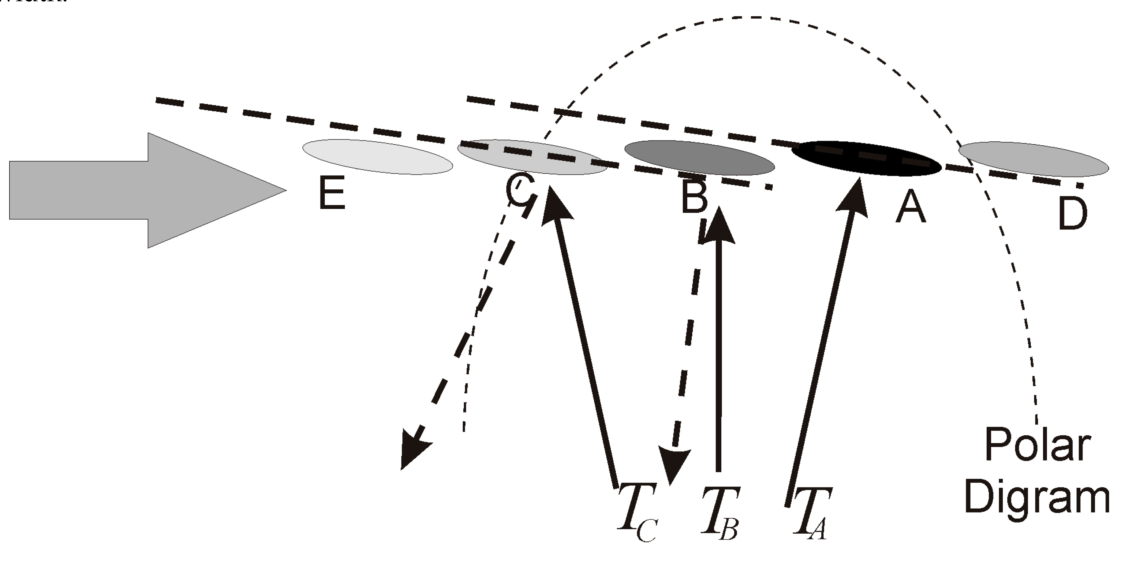
Now consider scatter from the beams. Pulses from the transmitter are transmitted radially, and will follow trajectories represented by TA, TB and TC as examples. Each strikes a different eddy (or, if there is only one eddy, the radar-paths strike the eddy at different times). Due to the alignment of eddy “A”, it reflects most of its energy back to the receiver. But eddies B and C reflect energy off-axis and so the signal received at the radar will be diminished.(While we speak of “reflection”, in reality the process should be treated as a scattering process, as in [19,37,38], but this simple colloquial discussion is adequate here).
From Figure 9, then scatter will be strongest from eddy “A”, and the more oblate the ellispoids, the more dominant will be the effect of eddy “A”.
Hence despite the fact that the eddy moves uniformly through the beam, scatter will be dominated by eddy “A” due to its alignment. The radial component of velocity at this point will be positive (away from the antenna aray), and so the Fourier spectrum of the time-series will be dominated by positive frequencies. Hence the radar analysis will produce a positive velocity, even though there is no vertical motion. Furthermore, the radial velocity “measured” will be proportional to the horizontal wind. This is all consistent with our studies.
At the current point in time, this model seems to best explain our data. Turbulence is a frequent occurrence in the atmosphere, so the radar-effects produced by this mechanism can easily persist over the course of months and years, as seen in our results. Not only does the model match our data, but our data allows us to quantify the mean eddy-tilting in patches of turbulence to an accuracy of 0.2o and better - a new capability not previously available, and giving new insights into the nature of atmospheric turbulence!
Three final comments need to be made. First, we should note that the “tilt angle” we measure will be moderated by the beam itself (see Figure 9), and some of the larger angles could even be a little larger in reality. Correction of the measured tilt to produce the true tilt is beyond the scope of this paper, though techniques like those presented in [19,37,38] can be used to make these adjustments.
Second, we should also note that many previous authors have used vertical velocities measured with a vertical beam to study short-term gravity wave activity. As long as the mean wind is relatively constant during the study, or has an identifiable behaviour, then the effects presented in this paper can be successfully removed, and the remaining short-term fluctuations can still be used for gravity-wave studies. However, studies of long-term behaviour of the mean vertical wind must include corrections for the effects presented here-in.
As a final (third) point of interest, it is interesting to compare the results here to the results from [29]. That paper looked at the distribution of regions in the atmosphere where gravity waves dominatedm compared to regions where large-scale 2-D geostrophic turbulence was more prevalent. Both Walsingham and Harrow appeared to have significant gravity wave production, especially in Summer, due presumably to lake breezes. Both sites showed more gravity waves than the other sites used in that study, and both show significant wave production in the lowest 2 km. Comparing these results to Figure 8 here-in, it is seen that our tilts become steeper at > 6 km in Summer at Harrow, and at 6-9 km at Walsingham. These results would be consistent with gravity wave production near the ground, free growth to ~6 km altitude, then breaking of the waves to produce strong turbulence and subsequent secondary gravity-wave growth at 6 km and upward. The large-ish layer tilts seen in Figure 8 of this paper occurring at similar heights to the active gravity-wave growth at 6 km may be further support for our model.
6. Conclusions
Extensive investigations with 6 radars over a time-frame of up to 4 years show significant correlation between long-term vertical and horizontal winds as measured by VHF radar. Interpretation of these data leads to the conclusion that scatter on the vertical radar beam is biased due to mean tilts in the scattering entities of the order of 0.5 to 2.5 degrees, and at times more. Extensive statistical tests confirm that these measurements are not artefacts, and significant variations are evident due to variations in season and local atmospheric conditions. Importantly, it is clear that anisotropic eddies within atmospheric turbulence are not on average flat, but have tilts of the order of a few degrees which depend on larger-scale influences like wind speed, wind shear and atmospheric stability (among others). The analysis method discussed in this paper has the unique potential to enable measurement of these tilts.
Acknowledgments
We would like to acknowledge the support of the Canada Foundation for Innovation (CFI), which funded the radar network construction, as well as support from the Natural Sciences and Engineering Research Council of Canada (NSERC). York University (through the CFI grant) administered construction of the radars, and all radars were built by Mardoc Inc. McGill University hosted the McGill windprofiler during its existence, and special support from Prof. F Fabry is recognized. Support of staff at all these institutions is acknowledged.
References
- Gage, K. S. and Green, J. L.: Evidence for specular reflection from monostatic VHF radar observations of the stratosphere, Radio Sci., 13, 991–1001, 1978. [CrossRef]
- Röttger, J. and Liu, C. H.: Partial reflection and scattering of VHF radar signals from the clear atmosphere, Geophys. Res. Lett., 5, 357–360, 1978. [CrossRef]
- Doviak, R., and D. Zrnic, Reflection and scatter formula for anisotropically turbulent air, Rad.Sci., 19, 325–336, 1984.
- Woodman, R. F. and Chu, Y.: Aspect sensitivity measurements of VHF backscatter made with the Chung-Li radar: Plausible mechanisms, Radio Sci., 24, 113–125, 1989. [CrossRef]
- Röttger, J., Reflection and scattering of VHF radar signals from atmospheric refractivity structures, Radio Sci., 15, 259–276, 1980.
- Hocking, W.K., S. Fukao, T. Tsuda, M. Yamamoto, T. Sato and S. Kato, “Aspect sensitivity of stratospheric VHF radiowave scatterers, particularly above 15 km altitude”, Radio Sci., 25, 613-627, 1990.
- Dalaudier, F., Sidi, C., Crochet, M., and Vernin, J.: Direct Evidence of “Sheets” in the Atmospheric Temperature Field, J. Atmos. Sci., 51, 237–248, 1994. [CrossRef]
- Luce, H., Crochet, M., Dalaudier, F., and Sidi, C.: Interpretation of VHF ST radar vertical echoes from in situ temperature sheet observations, Radio Sci., 30, 1003–1025, 1995. [CrossRef]
- Luce, H., Kantha, L., Hashiguchi, H., Lawrence, D., Mixa, T., Yabuki, M., and Tsuda, T.: Vertical structure of the lower troposphere derived from MU radar, unmanned aerial vehicle, and balloon measurements during ShUREX 2015, Progress in Earth and Planetary Science, 5, 29, 2018. [CrossRef]
- Muschinski, A. and Wode, C.: First In Situ Evidence for Coexisting Submeter Temperature and Humidity Sheets in the Lower Free Troposphere, J. Atmos. Sci., 55, 2893–2906, 1998.
- Chimonas, G.: Steps, waves and turbulence in the stably stratified planetary boundary layer, Bound.-Lay. Meteorol., 90, 397–421, 1999. [CrossRef]
- Belova, E., J. Kero, S.P. Näsholm, E. Vorobeva, O.A. Godin, and V. Barabash, “Polar Mesosphere Winter Echoes and their relation to infrasound”, EGU General Assembly 2020, Online, 4–8 May 2020, EGU2020-5055, 2020. [CrossRef]
- Hooper, D. A., and L. Thomas, Aspect sensitivity of VHF scatterers in troposphere and stratosphere from comparison of powers in off-vertical beams, J. Atmos. Terr. Phys., 57, 655–663, 1995.
- Doddi, A., Lawrence, D., Fritts, D., Wang, L., Lund, T., Brown, W., Zajic, D., and Kantha, L.: Instabilities, Dynamics, and Energetics accompanying Atmospheric Layering (IDEAL): high-resolution in situ observations and modeling in and above the nocturnal boundary layer, Atmos. Meas. Tech., 15, 4023–4045, 2022. [CrossRef]
- Bolgiano, R. J., The general theory of turbulence - turbulence in the atmosphere, in Windsand turbulence in the stratosphere, mesosphere and ionosphere, edited by K. Rawer, pp.371–400, North Holland, Amsterdam, 1968.
- Hocking, W.K., S. Fukao, M. Yamamoto, T. Tsuda, and S. Kato, “Viscosity waves and thermal-conduction waves as a cause of ‘specular’ reflectors in radar studies of the atmosphere”, Radio Sci., 26, 1281-1303, 1991.
- Strelnikov, B., Tr. Staszak, R. Latteck, T. Renkwitz, I. Strelnikova, F.-J. Lübken, Baumgarten, J. Fiedler, J. L. Chau, J. Stude, M. Rapp, M. Friedrich, J. Gumbel, J. Hedin, E. Belova, M. Hörschgen-Eggers, G. Giono, I. Hörner, S. Löhle, M. Eberhart, S. Fasoulas, ‘“ounding rocket project ‘PMWE’ for investigation of polar mesosphere winter echoes”,J. Atmosph. Solar-Terr. Phys., 218, 2021, 105596, ISSN 1364-6826. [CrossRef]
- Gibson-Wilde, D., J. A. Werne, D. C. Fritts, and R. J. Hill, Direct numerical simulation of VHF radar measurements of turbulence in the mesosphere, Radio Sci., 35, 783–798, 2000.
- Briggs, B. H., and R. A. Vincent, Some theoretical considerations on remote probing of weakly scattering irregularities, Aust. J. Phys., 26, 805–814, 1973.
- Hocking, W.K., J. Röttger, R.D. Palmer, T. Sato and P.B. Chilson, “ Atmospheric Radar: Application and Science of MST Radars in the Earth’s Mesosphere, Stratosphere, Troposphere, and weakly ionized regions”, Cambridge University Press. ISBN 9781316556115, 2016. [CrossRef]
- McCullough, Emily M., Robin Wing, and James R. Drummond,. “The Relationship between Clouds Containing Multiple Layers 7.5–30 m Thick and Surface Weather Conditions” Atmosphere 12, no. 12: 1616, 2021. [CrossRef]
- Muschinski, A., Frehich, R., Jensen, M., Hugo, R., Hoff, A., Eaton, F., and Balsley, B.: Fine-Scale Measurements Of Turbulence In The Lower Troposphere: An Intercomparison Between a Kite- And Balloon-Borne, And A Helicopter-Borne Measurement System, Bound.-Lay. Meteorol., 98, 219–250, 2001 . [CrossRef]
- https://bpb-us-w2.wpmucdn.com/sites.uwm.edu/dist/8/663/files/2019/05/Mar7.pdf.
- Chilson, P. B., and G. Schmidt, Implementation of frequency domain interferometry at the SOUSY VHF radar: First results, Radio Sci., 31, 263–272, 1996.
- Chilson, P. B., S. Kirkwood, and I. Häggström, Frequency-domain interferometry mode observations of PMSE using the EISCAT VHF radar, Ann. Geophys., 18, 1599– 1612, 2001.
- Luce, H., M. K. Yamamoto, S. Fukao, D. Helal, and M. Crochet, A frequency domain radar interferometric imaging (FII) technique based on high resolution methods, J. Atmos. Solar-Terr. Phys., 63, 221–234, 2001.
- Farag, A., and W.K. Hocking, , “Correlation between vertical and horizontal winds in the troposphere as seen by the O-QNET”, Proc. of the Twelfth International Workshop on Technical and Scientific Aspects of MST Radar, London, Ont., Canada, May 17-23, 2009, eds. N. Swarnalingam and W.K. Hocking, 139-144, 2010. Published by The Canadian Association of Physics, ISBN 978-0-9867285-0-1.
- Hocking, A., and W.K. Hocking, “Tornado Identification and Forewarning with VHF Windprofiler radars”, Atmos. Sci. Letts., 19(1), 2018. [CrossRef]
- Hocking, W.K., S. Dempsey, M. C. Wright, P.A. Taylor and F. Fabry, “Studies of Relative Contributions of Internal Gravity Waves and 2-D Turbulence to Tropospheric and Lower Stratospheric Temporal Wind Spectra measured by a Network of VHF Windprofiler Radars using a Decade-long Data-set in Canada”, Q. J. R. Meteorol Soc., Vol. 147, Issue 740, 3735-3758, 2021. [CrossRef]
- Dehghan, A., W.K. Hocking and R. Srinivasan, “Comparisons between multiple in-situ aircraft turbulence measurements and radar in the troposphere”, J. Atmos. Solar-Terr. Phys., 118(A), 64-77, 2014. [CrossRef]
- Hocking, W.K., “System design, signal processing procedures and preliminary results for the Canadian (London, Ontario) VHF Atmospheric Radar”, Radio Sci., 32, 687-706, 1997.
- Hocking, W.K., T. Thayaparan, and S.J. Franke, “Method for statistical comparison of geophysical data by multiple instruments which have differing accuracies”, Adv. Space Res., 27, numbers 6-7, 1089-1098, 2001.
- Taylor, Peter A., Wensong Weng, Zheng Qi Wang, Mathew Corkum, Khalid Malik, Shama Sharma and Wayne Hocking, “Upper-Level Winds over Southern Ontario: O-QNet Wind Profiler and NARR Comparisons”, Atmosphere-Ocean, 55(1), 1-11, 2016. [CrossRef]
- Attarzadeh, Farnoush, “Studies of the Tilts of Atmospheric Scatterers by Windprofiler Radars” (2021). Electronic Thesis and Dissertation Repository. 7679, https://ir.lib.uwo.ca/etd/7679.
- Walterscheid, R.L. and W.K. Hocking, “Stokes diffusion by atmospheric internal gravity waves”, J. Atmos. Sci., 48, 2213-2230, 1991.
- Scorer, R. S., Dynamics of Meteorology and Climate, John Wiley, Chichester, England, 1997.
- Hocking, W.K., and A.M. Hamza, “A Quantitative measure of the degree of anisotropy of turbulence in terms of atmospheric parameters, with particular relevance to radar studies”, J. Atmos. Solar Terr. Phys., 59, 1011-1020, 1997.
- Vincent, R. A., The interpretation of some observations of radio waves scattered from the lower ionosphere, Aust. J. Phys., 26, 815–827, 1973.
Figure 1.
Some possible models of anisotropic and specular scatterers in the atmosphere: (a) entrainment, (b) vigorous mixing, (c) viscosity waves, (d)-(f) more realistic turbulence models.
Figure 1.
Some possible models of anisotropic and specular scatterers in the atmosphere: (a) entrainment, (b) vigorous mixing, (c) viscosity waves, (d)-(f) more realistic turbulence models.
Figure 2.
Pearson Correlation coefficients vs. azimuthal angle ϕ0 and altitude.
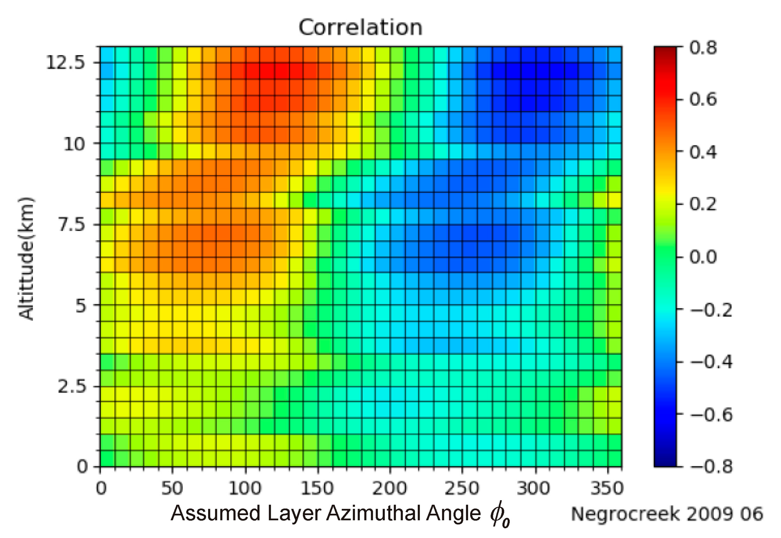
Figure 4.
Plots of (a) maximum correlation coefficient ,(b) azimuthal angle at which correlation maximizes, and (c) corresponding best-fit layer-tilt from horizontal (denoted θB, in degrees) for 2010 at the Harrow radar The first 2 graphs cover 13 months (including December in 2009) with altitudes from 0.5 to 13 km, while the layer-tilts cover January to October in 2010 at 0.5 km to 12.0 km. The first 2 graphs use the monthly colour-scale in the first panel, while the last graph uses its own colour panel.
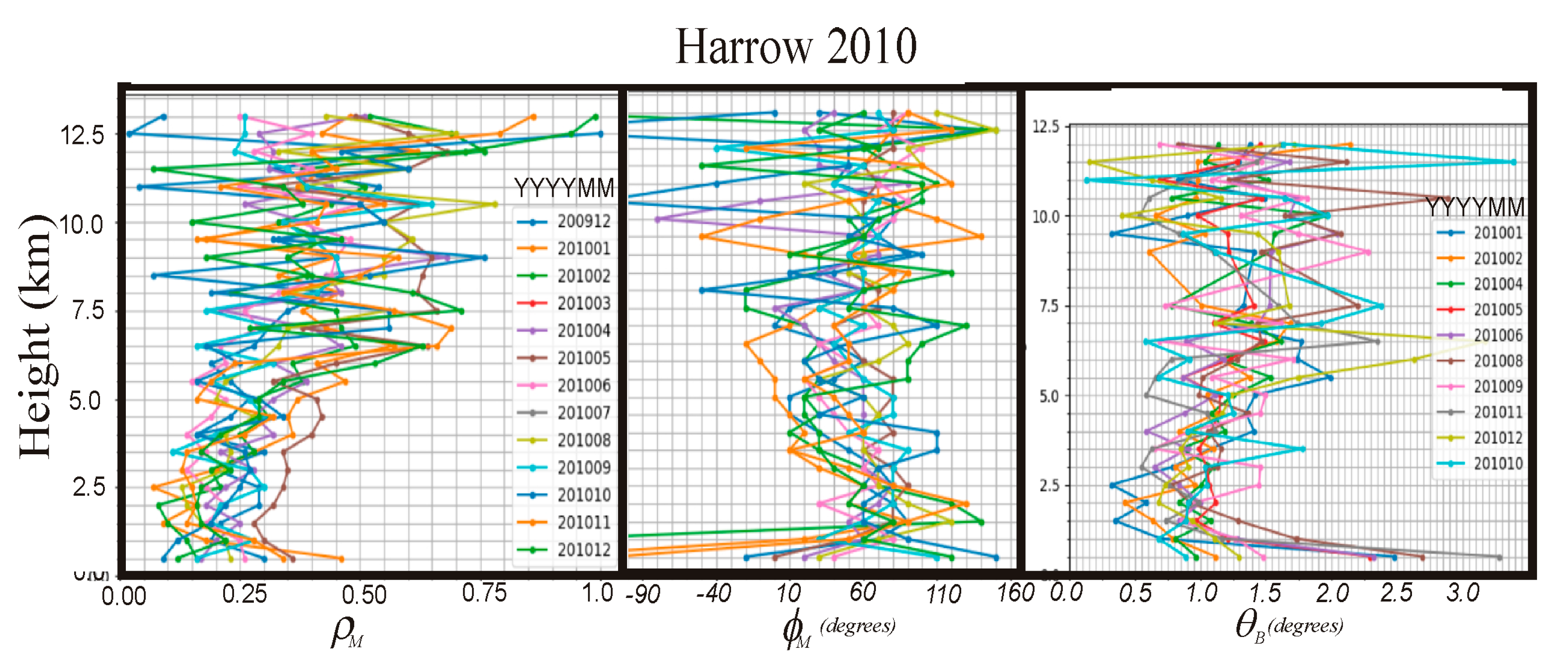
Figure 5.
Results of applying a 3-height × 3-month running average to correlation maxima like those shown in Figure 4(a). This graph applies to the Negro Creek site in 2010.
Figure 5.
Results of applying a 3-height × 3-month running average to correlation maxima like those shown in Figure 4(a). This graph applies to the Negro Creek site in 2010.
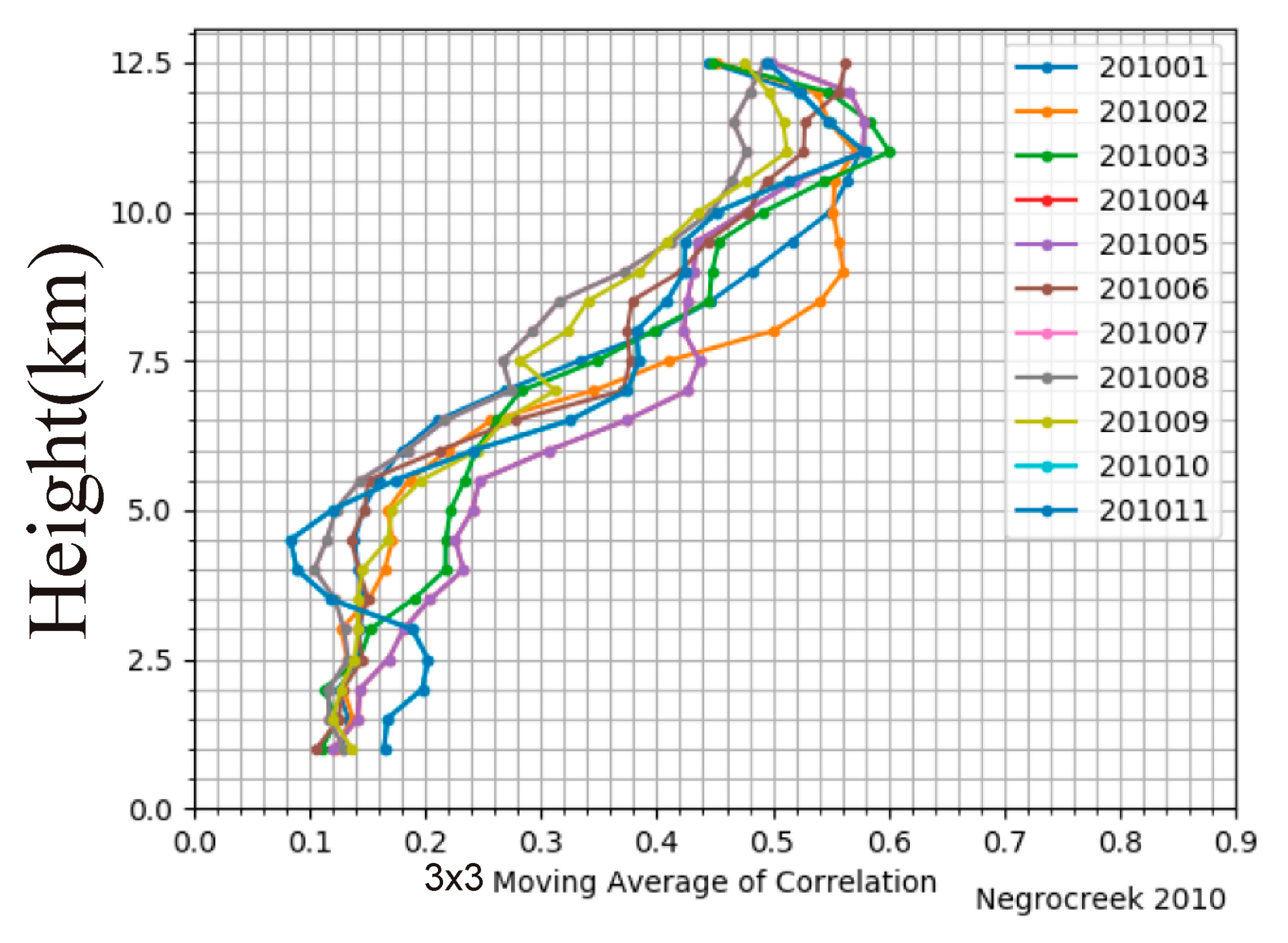
Figure 6.
Plots of azimuthal angle of alignment of the scattering layer (ϕΜ) as a function of height for the 6 sites used in this study. Sites are ranked according to latitude, with Eureka having the highest latitude (polar site at 80oN), then McGill having a latitude of 45.5oN, and then subsequent sites have decreasing latitude down to Harrow (42oN).
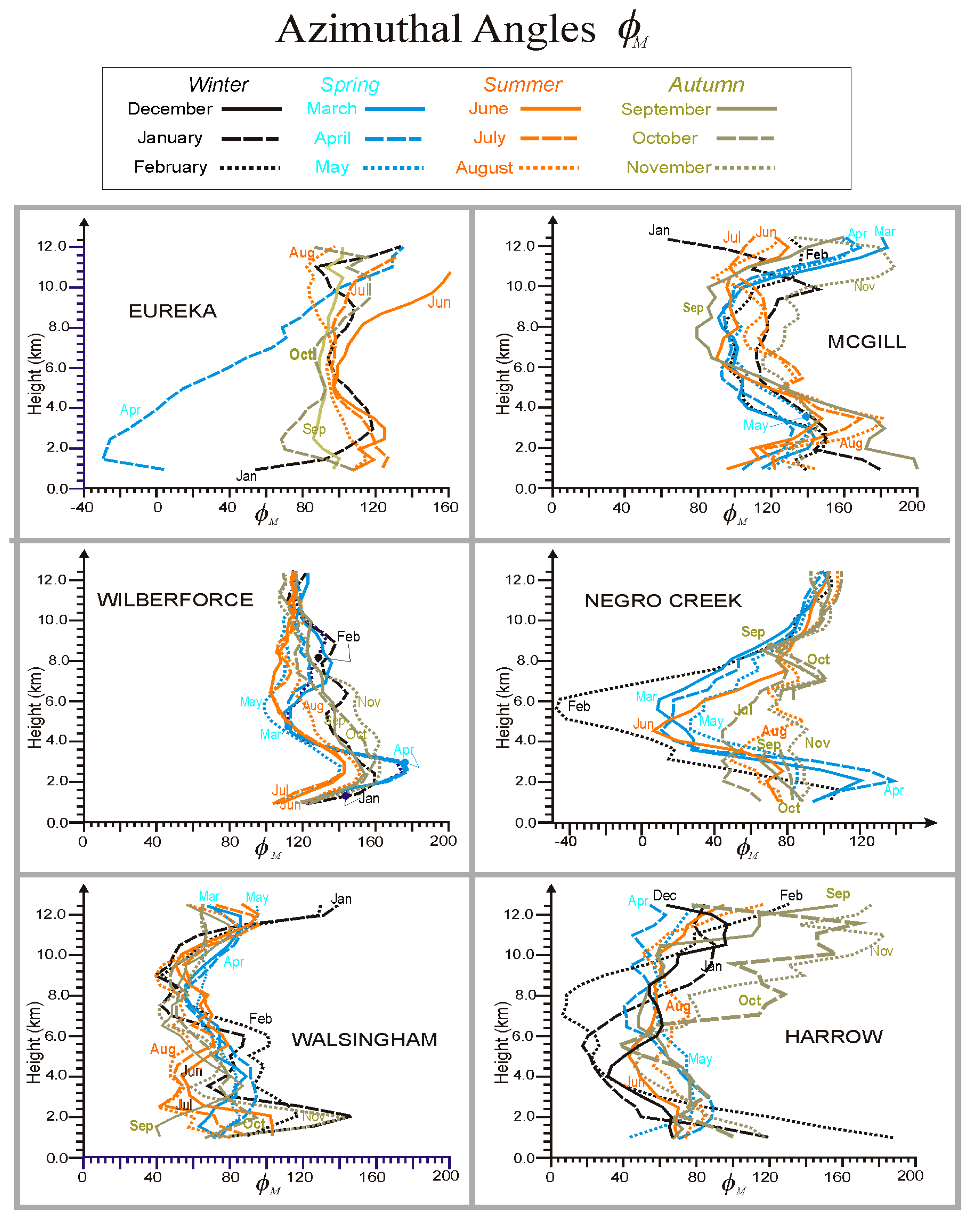
Figure 7.
Values of θB measured at Walsingham using 5point running averages over height, for the years of 2010, 2011, and 2012.
Figure 7.
Values of θB measured at Walsingham using 5point running averages over height, for the years of 2010, 2011, and 2012.
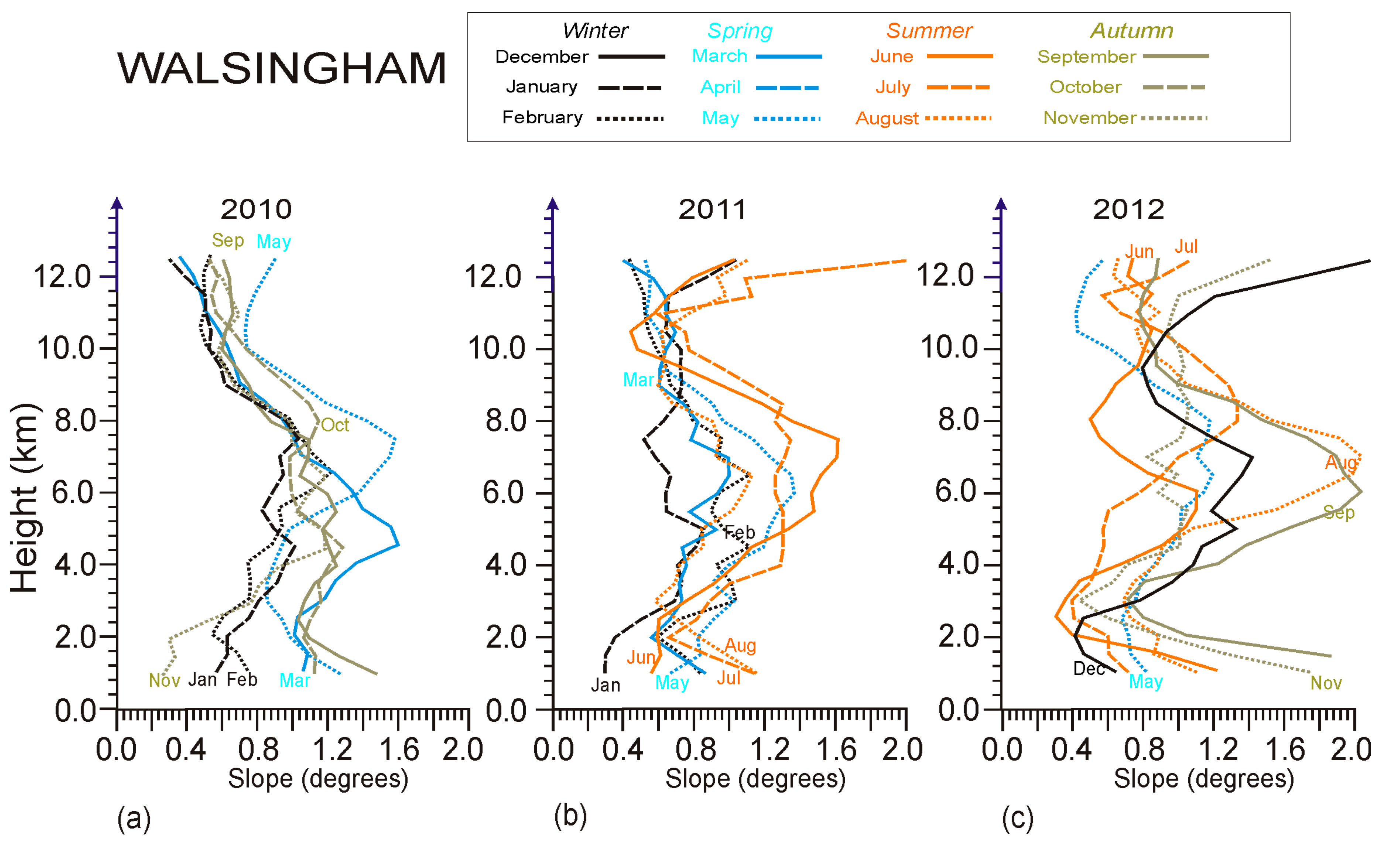
Figure 8.
Graphs of θB vs height using 3×3 running means over height and time (coupled with 5-point vertical running means in some cases) for all sites, as discussed in the text.
Figure 8.
Graphs of θB vs height using 3×3 running means over height and time (coupled with 5-point vertical running means in some cases) for all sites, as discussed in the text.
Disclaimer/Publisher’s Note: The statements, opinions and data contained in all publications are solely those of the individual author(s) and contributor(s) and not of MDPI and/or the editor(s). MDPI and/or the editor(s) disclaim responsibility for any injury to people or property resulting from any ideas, methods, instructions or products referred to in the content. |
© 2024 by the authors. Licensee MDPI, Basel, Switzerland. This article is an open access article distributed under the terms and conditions of the Creative Commons Attribution (CC BY) license (http://creativecommons.org/licenses/by/4.0/).
Copyright: This open access article is published under a Creative Commons CC BY 4.0 license, which permit the free download, distribution, and reuse, provided that the author and preprint are cited in any reuse.


