
Submitted:
18 November 2024
Posted:
20 November 2024
You are already at the latest version
Abstract
Many studies aim to assess the characteristics of blue-green infrastructure (BGI) that influence its cooling potential. Commonly used methods include satellite remote sensing, numerical simulations, and field measurements, each defining different cooling efficiency indicators. However, the methodological diversity creates uncertainties in optimizing BGI planning and management. This gap was addressed through a literature review, examining how BGI cools urban space, which spatial data and methods are most effective, which methodological differences may affect the results, and what are current research gaps and innovative future directions. Results suggest that differences in conclusions may arise from geographic and seasonal variations, as well as the spatial resolution of data, model scale, BGI delineation method, cooling range calculation approach, and urban morphology differences. The most influencing BGI characteristics include object size, vegetation fraction, density, height and multi-layering, foliage density, and spatial connectivity. The role of shape complexity remains uncertain across methodological approaches. Future research should prioritize the effects of urban morphology on BGI characteristics effectiveness and explore innovative approaches like Digital Twin technology for BGI management optimization. This paper comprehensively integrates key information related to BGI's cooling capabilities, serving as a useful resource for both practitioners and researchers to support resilient cities development.
Keywords:
1. Introduction and Background
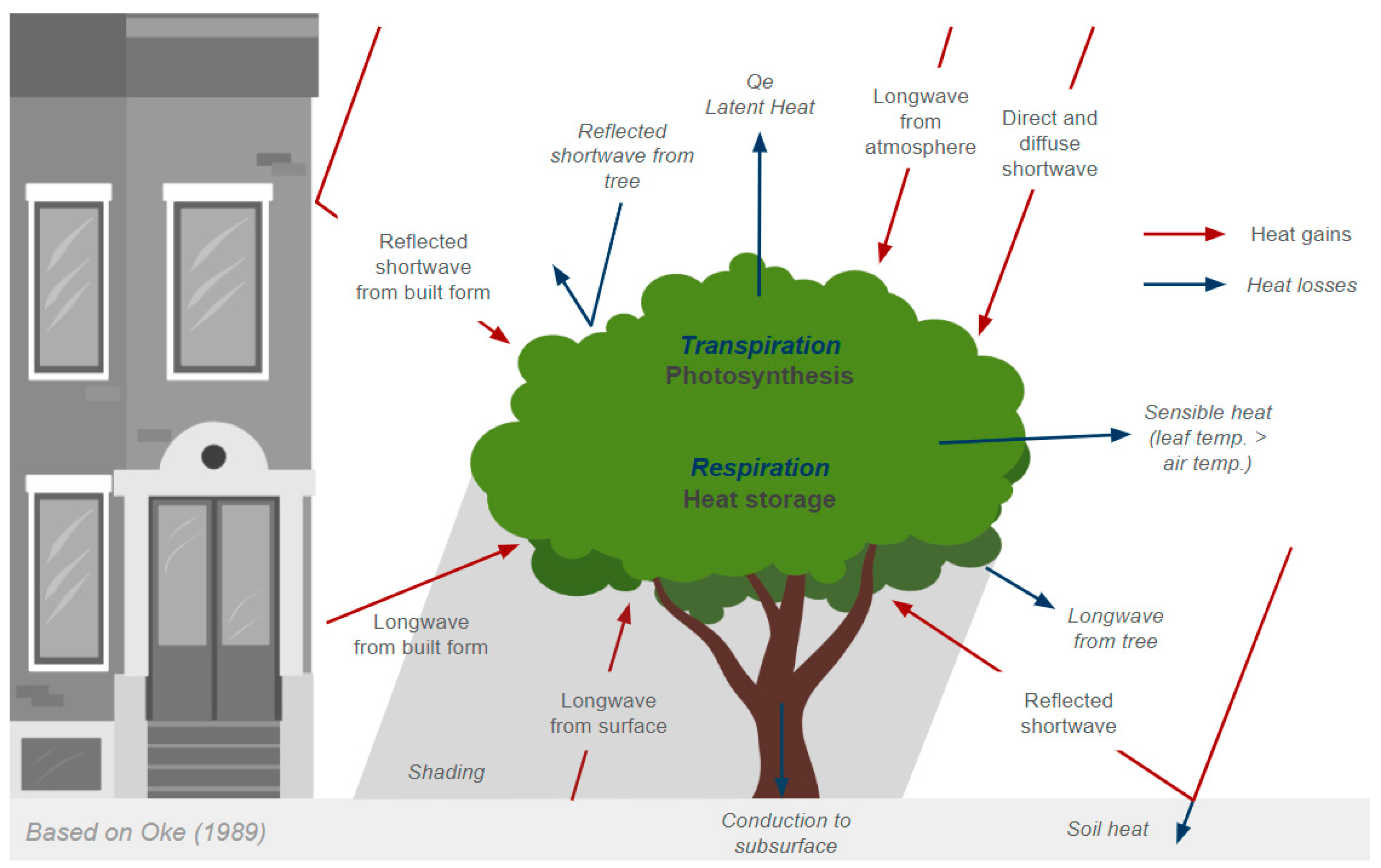
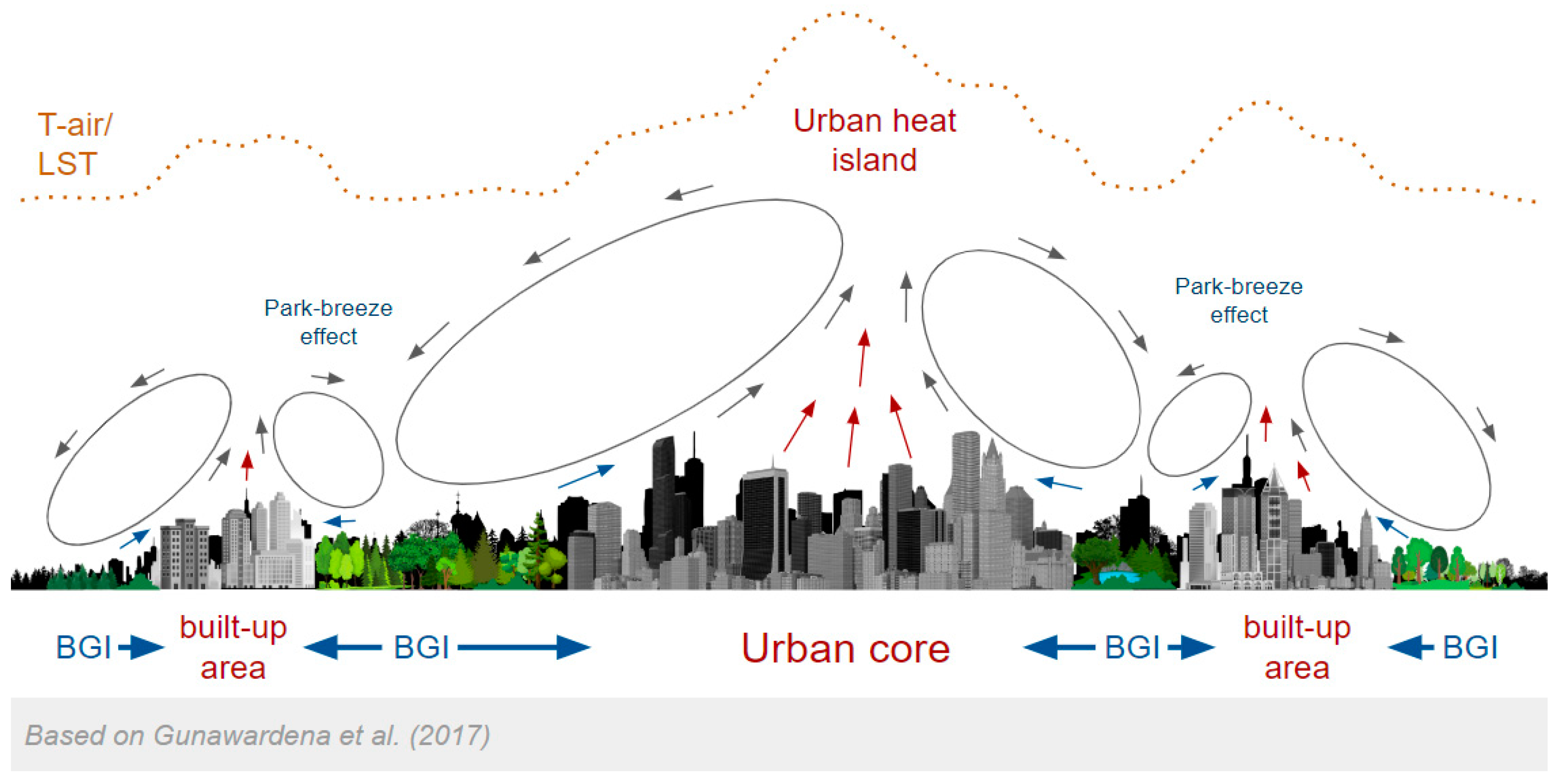
- Presenting the mechanisms behind the formation of BGI's cooling abilities;
- Discussing the most effective BGI features that positively impact cooling potential regardless of method;
- Examining the characteristics of spatial data and geoinformatics methods used in analyzing BGI's cooling effects, with attention to potential impacts on result variability;
- Proposing promising future research directions for optimizing BGI planning and management processes.
2. Materials and Methods
3. Existing Methods for Assessing the Thermal Characteristics of Urban Areas
4. Factors Determining the Cooling Potential of BGI
4.1. Micro-Scale Properties of BGI Affecting Cooling Potential
4.2. Local-Scale Properties of Bgi Affecting Cooling Potential
4.3. Urban Morphology Impact
5. Characteristics of Selected Geoinformatics Methods and Spatial Data Used to Assess the Cooling Potential of BGI
5.1. UCI Studies Based on Satellite Remote Sensing
5.1.1. Methods for Creating BGI Representation
5.1.2. Methods for Assessing the Cooling Potential of BGI
5.1.3. Remote Sensing Data Used in UCI Studies
5.2. UCI Studies Based on Numerical Simulations
5.2.1. Methods for Creating BGI Representation
5.2.2. Methods for Assessing the Cooling Potential of BGI
5.2.3. Data Used for ENVI-Met Simulation
5.3. UCI Studies Based on Field Measurements
6. Technologies with the Potential to Develop Tools to Optimize BGI Planning and Management
7. Discussion
7.1. Interpretation and Findings
7.1.1. Differences Between Results Obtained Using Different Approaches
7.1.2. BGI Characteristics Affecting Cooling Potential
7.2. Gaps and Future Research Directions
7.2.1. Incorporating Factors Related to Urban Morphology Around BGI
7.2.2. Development of an Objective Method for Delimiting BGI Objects for Analysis
7.2.3. Integration of New Spatial Data
7.2.4. Research on a Large Scale or the Integration of Results into a Universal Indicator
7.2.5. Correct Interpretation of Results Obtained Using LST
7.2.6. Development of Comprehensive Urban Ventilation Models
7.2.7. Use of the Digital Twin Technology
8. Conclusions
Author Contributions
Funding
Data Availability Statement
Conflicts of Interest
References
- Easterling, D. R.; et al. Climate Extremes: Observations, Modeling, and Impacts. Science 2000, 289. [Google Scholar] [CrossRef] [PubMed]
- Stephenson, D. Definition, diagnosis, and origin of extreme weather and climate events;, 2008. [CrossRef]
- Meehl, G.A. and Tebaldi, C. More Intense, More Frequent, and Longer Lasting Heat Waves in the 21st Century. Science 2004, 305. [CrossRef]
- Meehl, G. A.; et al. An introduction to trends in extreme weather and climate events: Observations, socioeconomic impacts, terrestrial ecological impacts, and model projections. B Am Meteorol Soc. 2000, 81. [Google Scholar] [CrossRef]
- D'Ippoliti, D. The impact of heat waves on mortality in 9 European cities: Results from the EuroHEAT project. Environmental health: a global access science source 2010, 9. [CrossRef]
- Semenza, J. C.; et al. Heat-related deaths during the July 1995 heat wave in Chicago. N Engl J Med 1996, 335. [Google Scholar] [CrossRef]
- Kotz, M.; et al. The economic commitment of climate change. Nature 2024, 628. [Google Scholar] [CrossRef] [PubMed]
- Newman, R. The global costs of extreme weather that are attributable to climate change. Nature Communications 2023, 14. [Google Scholar] [CrossRef]
- Maxwell, S.; et al. Conservation implications of ecological responses to extreme weather and climate events. Diversity and Distributions 2018, 25. [Google Scholar] [CrossRef]
- Garrabou, J.; et al. Mass mortality in Northwestern Mediterranean rocky benthic communities: effects of the 2003 heat wave. Global Change Biology 2009, 15. [Google Scholar] [CrossRef]
- Howard, L. The climate of London: deduced from meteorological observations made in the metropolis and at various places around it, London, 1833.
- Sundborg, A. A. Climatological Studies in Uppsala. With Special Regard to the Temperature Conditions in the Urban Area; Appelbergs Boktryckeri Aktiebolag, Uppsala, 1951.
- Oke, T. R. The energetic basis of urban heat island. Quarterly Journal of the Royal Meteorological Society 1982, 108. [Google Scholar] [CrossRef]
- Oke, T. R. City size and the urban heat island. Atmospheric Environment 1973, 7. [Google Scholar] [CrossRef]
- Kalnay, E. and Cai, M. Impact of Urbanization and Land-Use Change on Climate. Nature 2003, 423. [CrossRef]
- McCarthy, M. P.; et al. Climate change in cities due to global warming and urban effects. Geophysical Research Letters 2010, 37. [Google Scholar] [CrossRef]
- Bazrkar, M. H.; et al. Urbanization and Climate Change; In: Leal Filho, W. (eds) Handbook of Climate Change Adaptation. Springer, Berlin, Heidelberg. 2015. [Google Scholar] [CrossRef]
- Qian, Y.; et al. Urbanization Impact on Regional Climate and Extreme Weather: Current Understanding, Uncertainties, and Future Research Directions. Adv Atmos Sci. 2022, 39. [Google Scholar] [CrossRef] [PubMed]
- Intergovernmental Panel on Climate Change (IPCC). Summary for Policymakers. In: Climate Change 2021 – The Physical Science Basis: Working Group I Contribution to the Sixth Assessment Report of the Intergovernmental Panel on Climate Change; Cambridge University Press, 2023. [CrossRef]
- Zhan, Y.; et al. Urbanization can accelerate climate change by increasing soil N2O emission while reducing CH4 uptake. Global Change Biology 2023, 29. [Google Scholar] [CrossRef] [PubMed]
- Tan, J.; et al. The urban heat island and its impact on heat waves and human health in Shanghai. Int J Biometeorol 2010, 54. [Google Scholar] [CrossRef] [PubMed]
- European Commission. COMMUNICATION FROM THE COMMISSION TO THE EUROPEAN PARLIAMENT, THE COUNCIL, THE EUROPEAN ECONOMIC AND SOCIAL COMMITTEE AND THE COMMITTEE OF THE REGIONS. Green Infrastructure (GI) – Enhancing Europe’s Natural Capital 2013, 41400.
- Givoni, B. Impact of planted areas on urban environmental quality: A review. Atmospheric Environment. Part B. Urban Atmosphere 1991, 25. [Google Scholar] [CrossRef]
- Gill, S.; et al. Adapting Cities for Climate Change: The Role of the Green Infrastructure. Built Environment 2007, 33. [Google Scholar] [CrossRef]
- Monteiro, R.; et al. Green Infrastructure Planning Principles: An Integrated Literature Review. Land 2020, 9. [Google Scholar] [CrossRef]
- Costanza, R.; et al. The value of the world’s ecosystem services and natural capital. Nature 1996, 387. [Google Scholar]
- Almaaitah, T.; et al. The potential of Blue-Green infrastructure as a climate change adaptation strategy: a systematic literature review. Blue-Green Systems 2021, 3. [CrossRef]
- Reid, W. V.; et al. Millennium Ecosystem Assessment. Ecosystems and Human Well-being: synthesis; Island Press, 2005.
- Voskamp, I.M. and Van de Ven, F. H. M. Planning support system for climate adaptation: Composing effective sets of blue-green measures to reduce urban vulnerability to extreme weather events. Building and Environment 2015, 83. [CrossRef]
- Demuzere, M.; et al. Mitigating and adapting to climate change: Multi-functional and multi-scale assessment of green urban infrastructure. Journal of environmental management 2014, 146. [Google Scholar] [CrossRef]
- Januchta-Szostak, A. Błękitno-zielona infrastruktura jako narzędzie adaptacji miast do zmian klimatu w zagospodarowania wód opadowych. Architektura, Urbanistyka, Architektura Wnętrz 2020, 3. [CrossRef]
- Jim, C. Y.; et al. Charting the green and climate-adaptive city. Landscape and Urban Planning 2015, 138. [Google Scholar] [CrossRef]
- Spronken-Smith, R.A. and Oke, T. R. The Thermal Regime of Urban Parks in Two Cities with Different Summer Climates. International Journal of Remote Sensing 1998, 19. [Google Scholar] [CrossRef]
- Chang, C. R.; et al. A preliminary study on the cool-island intensity of Taipei city parks. Landscape and Urban Planning 2007, 80. [Google Scholar] [CrossRef]
- Yang, X.; et al. The urban cool island phenomenon in a high-rise high density city and its mechanisms. International Journal of Climatology 2017, 37. [Google Scholar] [CrossRef]
- Zhao-wu, Y. U.; et al. Impacts of urban cooling effect based on landscape scale: A review. Chinese Journal of Applied Ecology 2015, 26. [Google Scholar]
- Xie, Q.; et al. Regulation of water bodies to urban thermal environment: Evidence from Wuhan, China. Frontiers in Ecology and Evolution 2023, 11. [Google Scholar] [CrossRef]
- Anjos, M. and Lopes, A. Urban Heat Island and Park Cool Island Intensities in the Coastal City of Aracaju, North-Eastern Brazil. Sustainability 2017, 9. [CrossRef]
- Ren, Z.; et al. Estimation of the Relationship between Urban Park Characteristics and Park Cool Island Intensity by Remote Sensing Data and Field Measurement. Forests 2013, 4. [Google Scholar] [CrossRef]
- Kong, F.; et al. Effects of spatial pattern of greenspace on urban cooling in a large metropolitan area of eastern China. Landscape and Urban Planning 2014, 128. [Google Scholar] [CrossRef]
- Yu, Z.; et al. How can urban green spaces be planned for climate adaptation in subtropical cities? Ecological Indicators 2017, 82. [Google Scholar] [CrossRef]
- Krayenhoff, E. S.; et al. Cooling hot cities: A systematic and critical review of the numerical modelling literature. Environmental Research Letters 2021, 16. [Google Scholar] [CrossRef]
- Zhou, D.; et al. Satellite Remote Sensing of Surface Urban Heat Islands: Progress, Challenges, and Perspectives. Remote Sensing 2019, 11. [Google Scholar] [CrossRef]
- Bahi, H.; et al. Review of methods for retrieving urban heat islands. Materials Today: Proceedings 2020, 27. [CrossRef]
- Voogt, J.A. and Oke, T. R. Thermal remote sensing of urban climates. Remote Sensing of Environment 2003, 86. [Google Scholar] [CrossRef]
- Oyler, J. W.; et al. Remotely sensed land skin temperature as a spatial predictor of air temperature across the conterminous United States. Journal of Applied Meteorology and Climatology 2016, 55. [Google Scholar] [CrossRef]
- Good, E. An in situ-based analysis of the relationship between land surface “skin” and screen-level air temperatures: Land Skin-Air Temperature Relationship. Journal of Geophysical Research: Atmospheres 2016, 121. [CrossRef]
- Mirzaei, P.A. and Haghighat, F. Approaches to study urban heat island–abilities and limitations. Building and environment 2010, 45. [CrossRef]
- Becker, F. and Li, Z. L. Surface temperature and emissivity at various scales: Definition, measurement and related problems. Remote sensing reviews 1995, 12. [CrossRef]
- Hulley, G.C. and Ghent, D. Taking the Temperature of the Earth: Steps towards Integrated Understanding of Variability and Change; Elsevier: Amsterdam, The Netherlands. 2019.
- Hulley, G.; et al. New ECOSTRESS and MODIS Land Surface Temperature Data Reveal Fine-Scale Heat Vulnerability in Cities: A Case Study for Los Angeles County, California. Remote Sensing 2019, 11. [Google Scholar] [CrossRef]
- Li, C. and Yu, C. W. Mitigation of urban heat development by cool island effect of green space and water body; Proceedings of the 8th International Symposium on Heating, Ventilation and Air Conditioning, Springer, 2014. [CrossRef]
- O'Malley, C.; et al. Urban Heat Island (UHI) mitigating strategies: A case-based comparative analysis. Sustainable Cities and Society 2015, 19. [Google Scholar] [CrossRef]
- Qiu, G. Y.; et al. Experimental studies on the effects of green space and evapotranspiration on urban heat island in a subtropical megacity in China. Habitat International 2017, 68. [Google Scholar] [CrossRef]
- Yu, Z.; et al. Critical review on the cooling effect of urban blue-green space: A threshold size perspective. Urban Forestry and Urban Greening 2020, 49. [Google Scholar] [CrossRef]
- O'Malley, C.; et al. Urban Heat Island (UHI) mitigating strategies: a case-based comparative analysis. Sustainable Cities and Society 2015, 19. [Google Scholar] [CrossRef]
- Du, H.; et al. Research on the cooling island effects of water body: A case study of Shanghai, China. Ecol. Indic. 2016, 67. [Google Scholar] [CrossRef]
- Yang, G.; et al. How can urban blue-green space be planned for climate adaption in high-latitude cities? Sustainable Cities and Society 2020, 53. [Google Scholar] [CrossRef]
- Qiu, X.; et al. Cooling Effect of Urban Blue and Green Spaces: A Case Study of Changsha, China. Int. J. Environ. Res. Public Health 2023, 20. [Google Scholar] [CrossRef]
- Gao, Y.; et al. Analysis of the spillover characteristics of cooling effect in an urban park: A case study in Zhengzhou city. Front. Earth Sci 2023, 11. [Google Scholar] [CrossRef]
- Yao, X.; et al. How can urban parks be planned to mitigate urban heat island effect in “Furnace cities”? Journal of Cleaner Production 2022, 330. [Google Scholar] [CrossRef]
- Du, H.; et al. Quantifying the cool island effects of urban green spaces using remote sensing data. Urban For. Urban Green 2017, 27. [Google Scholar] [CrossRef]
- Tan, X.; et al. Comparison of cooling effect between green space and water body. Sustainable Cities and Society 2021, 67. [Google Scholar] [CrossRef]
- Liu, W.; et al. Green Space Cooling Effect and Contribution to Mitigate Heat Island Effect of Surrounding Communities in Beijing Metropolitan Area. Front. Public Health 2022, 10. [Google Scholar] [CrossRef] [PubMed]
- Kirschner, V.; et al. Measuring the relationships between various urban green spaces and local climate zones. Scientific Reports 2023, 13. [Google Scholar] [CrossRef]
- Sun, R.; et al. Cooling effects of wetlands in an urban region: The case of Beijing. Ecological Indicators 2012, 20. [Google Scholar] [CrossRef]
- Guo, F.; et al. Study on the mechanism of urban morphology on river cooling effect in severe cold regions. Frontiers in Public Health 2023, 11. [Google Scholar] [CrossRef]
- Verma, R.; et al. The relationship between spatial configuration of urban parks and neighbourhood cooling in a humid subtropical city. Landscape Ecology 2024, 39. [Google Scholar] [CrossRef]
- Skoulika, F.; et al. On the thermal characteristics and the mitigation potential of a medium size urban park in Athens, Greece. Landscape and Urban Planning 2014, 123. [Google Scholar] [CrossRef]
- Doick, K. J.; et al. The role of one large greenspace in mitigating London's nocturnal urban heat island. Science of The Total Environment 2014, 493. [Google Scholar] [CrossRef]
- Ca, V. T.; et al. Reductions in air conditioning energy caused by a nearby park. Energy and Buildings 1998, 29. [Google Scholar] [CrossRef]
- Jansson, C.; et al. Near surface climate in an urban vegetated park and its surroundings. Theor. Appl. Climatol. 2007, 89. [Google Scholar] [CrossRef]
- Lee, S. H.; et al. Effect of an urban park on air temperature differences in a central business district area. Landscape and Ecological Engineering 2009, 5. [Google Scholar] [CrossRef]
- Cohen, P.; et al. Daily and seasonal climatic conditions of green urban open spaces in the Mediterranean climate and their impact on human comfort. Building and Environment 2012, 51. [Google Scholar] [CrossRef]
- Oke, T. R. Boundary Layer Climates; Routledge, New York, 1987.
- Oke, T. R. The distinction between canopy and boundary-layer urban heat islands. Atmosfera 1976, 14. [Google Scholar] [CrossRef]
- Gunawardena, K. R.; et al. Utilising green and bluespace to mitigate urban heat island intensity. Science of The Total Environment 2017, 584–585. [Google Scholar] [CrossRef]
- Nichol, J. E.; et al. Urban heat island diagnosis using ASTER satellite images and ‘in situ’ air temperature. Atmospheric Research 2009, 94. [Google Scholar] [CrossRef]
- Schwarz, N.; et al. Relationship of land surface and air temperatures and its implications for quantifying urban heat island indicators—An application for the city of Leipzig (Germany). Ecological Indicators 2012, 18. [Google Scholar] [CrossRef]
- Smoliak, B. V.; et al. Dense Network Observations of the Twin Cities Canopy-Layer Urban Heat Island. Journal of Applied Meteorology and Climatology 2015, 54. [Google Scholar] [CrossRef]
- Chen, Q.; et al. Spatially explicit assessment of heat health risk by using multi-sensor remote sensing images and socioeconomic data in Yangtze River Delta, China. International Journal of Health Geographics 2018, 17. [Google Scholar] [CrossRef]
- Hussain, S.; et al. Relation of land surface temperature with different vegetation indices using multi-temporal remote sensing data in Sahiwal region, Pakistan; Geoscience Letters, 2023. [CrossRef]
- Zhao-Liang, L.; et al. Satellite-derived land surface temperature: Current status and perspectives. Remote Sensing of Environment 2013, 131. [Google Scholar] [CrossRef]
- Zhang, Y. and Sun, L. Spatial-temporal impacts of urban land use land cover on land surface temperature: Case studies of two Canadian urban areas. International Journal of Applied Earth Observation and Geoinformation 2019, 75. [CrossRef]
- Haynes, M. W.; et al. Australian mean land-surface temperature. Geothermics 2018, 72. [Google Scholar] [CrossRef]
- Pal, S. and Ziaul, S. Detection of land use and land cover change and land surface temperature in English Bazar urban centre. The Egyptian Journal of Remote Sensing and Space Sciences 2017, 20. [CrossRef]
- Rawat, V.; et al. Anomalous land surface temperature and outgoing long-wave radiation observations prior to earthquakes in India and Romania. Nat Hazards 2011, 59. [Google Scholar] [CrossRef]
- Li, Z. L.; et al. Satellite remote sensing of global land surface temperature: Definition, methods, products, and applications. Reviews of Geophysics 2023, 61. [Google Scholar] [CrossRef]
- Voogt, J.A. and Oke, T. R. Effects of urban surface geometry on remotely-sensed surface temperature. Int. J. Remote Sens. 1998, 19. [CrossRef]
- Voogt, J.A. and Oke, T. R. Complete Urban Surface Temperatures. J. Appl. Meteorol. 1997, 36. [Google Scholar] [CrossRef]
- Marzban, F.; et al. Estimation of the Near-Surface Air Temperature during the Day and Nighttime from MODIS in Berlin, Germany. Int. J. Adv. Remote Sens. GIS 2018, 7. [Google Scholar] [CrossRef]
- Good, E.; et al. A spatiotemporal analysis of the relationship between near-surface air temperature and satellite land surface temperatures using 17 years of data from the ATSR series. Journal of Geophysical Research: Atmospheres 2017, 122. [CrossRef]
- Bhandari, R.; et al. A Deep Neural Network-Based Approach for Studying the Relationship Between Land Surface Temperature and Surface Air Temperature. Journal of the Indian Society of Remote Sensing 2022, 50. [Google Scholar] [CrossRef]
- Arnfield, A. J. Two decades of urban climate research: a review of turbulence, exchanges of energy and water, and the urban heat island. International Journal of Climatology: a Journal of the Royal Meteorological Society 2003, 23. [CrossRef]
- Kloog, I.; et al. Predicting spatiotemporal mean air temperature using MODIS satellite surface temperature measurements across the Northeastern USA. Remote Sens. Environ. 2014, 150. [Google Scholar] [CrossRef]
- Oyler, J. W.; et al. Creating a topoclimatic daily air temperature dataset for the conterminous United States using homogenized station data and remotely sensed land skin temperature. Int. J. Climatol. 2015, 35. [Google Scholar] [CrossRef]
- Mildrexler, D. J.; et al. A global comparison between station air temperatures and MODIS land surface temperatures reveals the cooling role of forests. J. Geophys. Res. Biogeosci. 2011, 116. [Google Scholar] [CrossRef]
- Benali, A.; et al. Estimating air surface temperature in Portugal using MODIS LST data. Remote Sensing of Environment 2012, 124. [Google Scholar] [CrossRef]
- Noi, P. T.; et al. Comparison of Multiple Linear Regression, Cubist Regression, and Random Forest Algorithms to Estimate Daily Air Surface Temperature from Dynamic Combinations of MODIS LST Data. Remote Sens. 2017, 9. [Google Scholar] [CrossRef]
- Rosselló, C.; et al. Modeling air temperature through a combination of remote sensing and GIS data. Journal of Geophysical Research 2008, 113. [Google Scholar] [CrossRef]
- Pichierri, M.; et al. Satellite air temperature estimation for monitoring the canopy layer heat island of Milan. Remote Sens. Environ. 2012, 127. [Google Scholar] [CrossRef]
- Ho, H. C.; et al. Mapping maximum urban air temperature on hot summer days. Remote Sensing of Environment 2014, 154. [Google Scholar] [CrossRef]
- Ding, X.; et al. Machine learning-assisted mapping of city-scale air temperature: Using sparse meteorological data for urban climate modeling and adaptation. Building and Environment 2023, 234. [Google Scholar] [CrossRef]
- Venter, Z.; et al. Hyperlocal mapping of urban air temperature using remote sensing and crowdsourced weather data. Remote Sensing of Environment 2020, 242. [Google Scholar] [CrossRef]
- Howard, H. H. Computational Fluid Dynamics; In book: Fluid Mechanics. 2012. [Google Scholar] [CrossRef]
- Toparlar, Y.; et al. A review on the CFD analysis of urban microclimate. Renewable and Sustainable Energy Reviews 2017, 80. [Google Scholar] [CrossRef]
- Liu, Z.; et al. Heat mitigation benefits of urban green and blue infrastructures: A systematic review of modeling techniques, validation and scenario simulation in ENVI-met V4. Building and Environment 2021, 200. [Google Scholar] [CrossRef]
- Yang, Y.; et al. The “plant evaluation model” for the assessment of the impact of vegetation on outdoor microclimate in the urban environment. Building and Environment 2019, 159. [Google Scholar] [CrossRef]
- Kumar, P.; et al. Nature-based solutions efficiency evaluation against natural hazards: Modelling methods, advantages and limitations. Science of The Total Environment 2021, 784. [Google Scholar] [CrossRef] [PubMed]
- Azmeer, A.; et al. Progress on green infrastructure for urban cooling: Evaluating techniques, design strategies, and benefits. Urban Climate 2024, 56. [Google Scholar] [CrossRef]
- Skamarock, W.C. and Klemp, J. B. A time-split nonhydrostatic atmospheric model for weather research and forecasting applications. Journal of Computational Physics 2008, 227. [CrossRef]
- Taha, H. Urban Climates and Heat Islands; Albedo, Evapotranspiration, and Anthropogenic Heat. Energy and Buildings 1997, 25. [Google Scholar] [CrossRef]
- Taha, H.; et al. Residential cooling loads and the urban heat island—the effects of albedo. Building and Environment 1988, 23. [Google Scholar] [CrossRef]
- Shashua-Bar, L.; et al. The cooling efficiency of urban landscape strategies in a hot dry climate. Landscape and Urban Planning 2009, 92. [Google Scholar] [CrossRef]
- Mariani, L.; et al. Climatological analysis of the mitigating effect of vegetation on the urban heat island of Milan, Italy. Science of The Total Environment 2016, 569–570. [Google Scholar] [CrossRef]
- Oke, T. R. The micrometeorology of the urban forest. Philos. Trans. R. Soc. Lond. Ser. B Biol. Sci. 1989, 324. [Google Scholar] [CrossRef]
- Armson, D.; et al. The effect of tree shade and grass on surface and globe temperatures in an urban area. Urban For. Urban Green. 2012, 11. [Google Scholar] [CrossRef]
- Shashua-Bar, L. and Hoffman, M. E. The Green CTTC model for predicting the air temperature in small urban wooded sites. Building and Environment 2002, 37. [Google Scholar] [CrossRef]
- Monteith, J. and Unsworth, M. Principles of Environmental Physics; Academic Press, an imprint of Elsevier, Oxford, 2013.
- Gill, S. E.; et al. Modelling water stress to urban amenity grass in Manchester UK under climate change and its potential impacts in reducing urban cooling. Urban For. Urban Green. 2013, 12. [Google Scholar] [CrossRef]
- Lloyd, M. K.; et al. Isotopic clumping in wood as a proxy for photorespiration in trees. Proceedings of the National Academy of Sciences 2023, 120. [Google Scholar] [CrossRef] [PubMed]
- Santamouris, M. Cooling the cities - a review of reflective and green roof mitigation technologies to fight heat island and improve comfort in urban environments. Solar Energy 2014, 103. [Google Scholar] [CrossRef]
- Bowler, D. E.; et al. Urban greening to cool towns and cities: A systematic review of the empirical evidence. Landscape and urban planning 2010, 97. [Google Scholar] [CrossRef]
- Zhang, L.; et al. Effects of the tree distribution and species on outdoor environment conditions in a hot summer and cold winter zone: A case study in Wuhan residential quarters. Building and Environment 2018, 130. [Google Scholar] [CrossRef]
- Zhao, Q.; et al. Impact of tree locations and arrangements on outdoor microclimates and human thermal comfort in an urban residential environment. Urban Forestry and Urban Greening 2018, 32. [Google Scholar] [CrossRef]
- McPherson, E. G.; et al. Chicago's Urban Forest Ecosystem: Results of the Chicago Urban Forest Climate Project; Gen. Tech. Rep. NE-186. Radnor, PA: U.S. Department of Agriculture, Forest Service, Northernestern Forest Experiment Station. 1994. [Google Scholar]
- Sun, R. and Chen, L. Landscape and Urban Planning 2012, 105. [Google Scholar] [CrossRef]
- Adams, L.W. and Dove, L. E. Wildlife Reserves and Corridors in the Urban Environment: A Guide to Ecological Landscape Planning and Resource Conservation; National Institute for Urban Wildlife, 1989.
- Webb, B.W. and Zhang, Y. Spatial and seasonal variability in the components of the river heat budget. Hydrol Process. 1997, 11.
- Hathway, E.A. and Sharples, S. The interaction of rivers and urban form in mitigating the urban heat island effect: a UK case study. Building and Environment 2012, 58. [CrossRef]
- Theeuwes, N. E.; et al. Modeling the influence of open water surfaces on the summertime temperature and thermal comfort in the city. J. Geophys. Res.: Atmos. 2013, 118. [CrossRef]
- Hathway, E.A. and Sharples, S. The interaction of rivers and urban form in mitigating the urban heat island effect: a UK case study. Build. Environ. 2012, 58. [CrossRef]
- Dong, J.; et al. Modelling air temperature gradients across managed small streams in western Washington. Journal of Environmental Management 1998, 53. [Google Scholar] [CrossRef]
- Hipsey, M.R. and Sivapalan, M. Parameterizing the effect of a wind shelter on evaporation from small water bodies. Water Resources Research. 2003, 39. [CrossRef]
- Jauregui, E. Influence of a large urban park on temperature and convective precipitation in a tropical city. Energy and Buildings 1990, 15. [Google Scholar] [CrossRef]
- Upmanis, H.; et al. The influence of green areas on nocturnal temperatures in a high latitude city (Göteborg, Sweden). International Journal of Climatology 1998, 18. [Google Scholar] [CrossRef]
- Jusuf, S.; et al. The influence of land use on the urban heat island in Singapore. Habitat International - HABITAT INT 2007, 31. [CrossRef]
- Lin, W.; et al. Calculating cooling extents of green parks using remote sensing: Method and test. Landscape and Urban Planning 2015, 134. [Google Scholar] [CrossRef]
- Eyster, H.N. and Beckage, B. Arboreal Urban Cooling Is Driven by Leaf Area Index, Leaf Boundary Layer Resistance, and Dry Leaf Mass per Leaf Area: Evidence from a System Dynamics Model. Atmosphere 2023, 14. [CrossRef]
- Li, H.; et al. Harnessing cooling from urban trees: Interconnecting background climates, urban morphology, and tree traits. EGUsphere 2024 [preprint]. [CrossRef]
- Trzeciak, M. and Sikorska, D. Application of UAV and ground measurements for urban vegetation cooling benefits assessment, Wilanów Palace case study. Scientific Review Engineering and Environmental Sciences 2024, 33. [CrossRef]
- Su, Y.; et al. Estimating the cooling effect magnitude of urban vegetation in different climate zones using multi-source remote sensing. Urban Climate 2022, 43. [Google Scholar] [CrossRef]
- Yu, Z.; et al. Strong contributions of local background climate to the cooling effect of urban green vegetation. Sci Rep 2018, 8. [Google Scholar] [CrossRef]
- Saaroni, H. and Ziv, B. The impact of a small lake on heat stress in a Mediterranean urban park: The case of Tel Aviv, Israel. International journal of biometeorology 2003, 47. [CrossRef]
- Pang, B.; et al. How to plan urban green space in cold regions of China to achieve the best cooling efficiency. Urban Ecosystems 2022, 25. [Google Scholar] [CrossRef]
- Huang, R.; et al. Cooling Effect of Green Space and Water on Urban Heat Island and the Perception of Residents: A Case Study of Xi’an City. International Journal of Environmental Research and Public Health (IJERPH) 2022, 19. [Google Scholar] [CrossRef]
- Hirai, H. and Kitaya, Y. Effects of Gravity on Transpiration of Plant Leaves. Annals of the New York Academy of Sciences 2009, 1161. [Google Scholar] [CrossRef]
- Zhaowu, Y.; et al. Enhanced observations from an optimized soil-canopy-photosynthesis and energy flux model revealed evapotranspiration-shading cooling dynamics of urban vegetation during extreme heat. Remote Sensing of Environment 2024. [CrossRef]
- Jaganmohan, M.; et al. The bigger, the better? J. Environ. Qual. 2016, 45. [Google Scholar] [CrossRef]
- Keramitsoglou, I.; et al. An online system for nowcasting satellite derived temperatures for urban areas. Remote Sens. 2016, 8. [Google Scholar] [CrossRef]
- Cai, Y.-B.; et al. Investigate the Difference of Cooling Effect between Water Bodies and Green Spaces: The Study of Fuzhou, China. Water 2022, 14. [Google Scholar] [CrossRef]
- Cao, B.; et al. Simulation Analysis of the Cooling Effect of Urban Water Bodies on the Local Thermal Environment. Water 2022, 14. [Google Scholar] [CrossRef]
- Murakawa, S.; et al. Study of the effects of a river on the thermal environment in an urban area. Energy Build. 1991, 16. [Google Scholar] [CrossRef]
- Hathway, E. and Sharples, S. The interaction of rivers and urban form in mitigating the Urban Heat Island effect: a UK case study. Build. Environ. 2012, 58. [CrossRef]
- Ellison, D.; et al. Trees, forests and water: cool insights for a hot world. Glob. Environ. Change. 2017, 43. [Google Scholar] [CrossRef]
- Du, H.; et al. A cold island connectivity and network perspective to mitigate the urban heat island effect. Sustainable Cities and Society 2023, 94. [Google Scholar] [CrossRef]
- Maimaitiyiming, M.; et al. Effects of green space spatial pattern on land surface temperature: Implications for sustainable urban planning and climate change adaptation. ISPRS Journal of Photogrammetry and Remote Sensing 2014, 89. [Google Scholar] [CrossRef]
- Bao, T.; et al. Assessing the Distribution of Urban Green Spaces and its Anisotropic Cooling Distance on Urban Heat Island Pattern in Baotou, China. ISPRS Int. J. Geo-Inf. 2016, 5. [CrossRef]
- Li, X.; et al. Spatial pattern of greenspace affects land surface temperature: evidence from the heavily urbanized Beijing metropolitan area, China. Landscape Ecol 2012, 27. [Google Scholar] [CrossRef]
- Nasar-u-Minallah, M.; et al. Evaluating the impact of landscape configuration, patterns and composition on land surface temperature: an urban heat island study in the Megacity Lahore, Pakistan. Environ Monit Assess 2024, 196. [Google Scholar] [CrossRef]
- Theeuwes, N.; et al. Modeling the influence of open water surfaces on the summertime temperature and thermal comfort in the city. J. Geophys. Res. Atmos. 2013, 118. [Google Scholar] [CrossRef]
- Liu, L.; et al. Cooling effects of wetland parks in hot and humid areas based on remote sensing images and local climate zone scheme. Building and Environment 2023, 243. [Google Scholar] [CrossRef]
- Stewart, I.D. and Oke, T. Local Climate Zones for Urban Temperature Studies. Bulletin of the American Meteorological Society 2012, 93. [Google Scholar] [CrossRef]
- Rogers, R.; et al. Urban Task Force, Towards an Urban Renaissance: Final Report of the Urban Task Force Chaired by Lord Rogers of Riverside; Department of the Environment, Transport and the Regions, London, 1999.
- Wong, N. H.; et al. Investigation of Thermal Benefits of Rooftop Garden in the Tropical Environment. Building and Environment 2003, 38. [Google Scholar] [CrossRef]
- Zhang, Y.; et al. Analysis of cold island effect in city parks from the perspectives of maximum and cumulative values – a case study of Xi'an City. Archives of Environmental Protection 2024, 50. [Google Scholar] [CrossRef]
- Feyisa, G. L.; et al. Efficiency of parks in mitigating urban heat island effect: An example from Addis Ababa. Landscape and Urban Planning 2014, 123. [Google Scholar] [CrossRef]
- Burton, E. Measuring urban compactness in UK towns and cities. Environment and Planning B: Planning and Design 2002, 29. [CrossRef]
- McPherson, E. G.; et al. Energy-efficient landscapes. In: Bradley, G. ed., Urban Forest Landscapes - Integrating Multidisciplinary Perspectives; University of Washington Press, Seattle, London, 1994.
- Yang, X.; et al. Air humidity characteristics of local climate zones: A three-year observational study in Nanjing. Building and Environment 2020, 175. [Google Scholar] [CrossRef]
- Zhao, Z.; et al. Local Climate Zone Classification Scheme Can Also Indicate Local-Scale Urban Ventilation Performance: An Evidence-Based Study. Atmosphere 2020, 11. [Google Scholar] [CrossRef]
- Alexander, P.J. and Mills, G. Local Climate Classification and Dublin’s Urban Heat Island. Atmosphere 2014, 5. [CrossRef]
- Ching, J.; et al. World Urban Database and Access Portal Tools (WUDAPT), an urban weather, climate and environmental modeling infrastructure for the Anthropocene. Bulletin of the American Meteorological Society 2018, 99. [Google Scholar] [CrossRef]
- Skarbit, N.; et al. Airborne surface temperature differences of the different Local Climate Zones in the urban area of a medium sized city; Joint Urban Remote Sensing Event (JURSE), 2015. [CrossRef]
- Geletič, J.; et al. Land Surface Temperature Differences within Local Climate Zones, Based on Two Central European Cities. Remote sensing 2016, 8. [Google Scholar] [CrossRef]
- Stewart, I. D.; et al. Evaluation of the 'local climate zone' scheme using temperature observations and model simulations. International Journal of Climatology 2014, 34. [Google Scholar] [CrossRef]
- Li, X.; et al. The role of blue green infrastructure in the urban thermal environment across seasons and local climate zones in East Africa. Sustainable Cities and Society 2022, 80. [Google Scholar] [CrossRef]
- Geletič, J.; et al. Inter-/intra-zonal seasonal variability of the surface urban heat island based on local climate zones in three central European cities. Building and Environment 2019, 156. [Google Scholar] [CrossRef]
- Wang, Y.; et al. Impact of Urban Climate Landscape Patterns on Land Surface Temperature in Wuhan, China. Sustainability 2017, 9. [Google Scholar] [CrossRef]
- Mohamed, A. A.; et al. Land surface temperature and emissivity estimation for Urban Heat Island assessment using medium-and low-resolution space-borne sensors: A review. Geocarto international 2017, 32. [Google Scholar] [CrossRef]
- Gorgani, S. A. et al. The Relationship between NDVI and LST in the urban area of Mashhad, Iran; Conference: International Conference on Civil Engineering Architecture and Urban Sustainable Development. 2012.
- Skelhorn, C.; et al. The impact of vegetation types on air and surface temperatures in a temperate city: A fine scale assessment in Manchester, UK. Landscape and Urban Planning 2014, 121. [Google Scholar] [CrossRef]
- Sun, M.; et al. Factors Affecting the High-Intensity Cooling Distance of Urban Green Spaces: A Case Study of Xi’an, China. Sustainability 2023, 15. [Google Scholar] [CrossRef]
- Huang, M.; et al. Study of the Cooling Effects of Urban Green Space in Harbin in Terms of Reducing the Heat Island Effect. Sustainability 2018, 10. [Google Scholar] [CrossRef]
- Oliver, M.A. and Webster, R. Kriging: a method of interpolation for geographical information systems. International Journal of Geographical Information Systems 1990, 4. [CrossRef]
- NASA. Thematic Mapper (TM). Available on-line: https://landsat.gsfc.nasa.gov/thematic-mapper/ (accessed on 5.06.2024).
- U.S. Geological Survey. Landsat-A Global Land-Imaging Mission: U.S. Geological Survey Fact Sheet 2012–3072: https://pubs.usgs.gov/fs/2012/3072/ (accessed on 5.06.2024).
- Wolf, T.; et al. Performance assessment of a heat wave vulnerability index for greater London, United Kingdom. Weather, climate, and society 2013. [CrossRef]
- Tomlinson, C. J.; et al. Including the urban heat island in spatial heat health risk assessment strategies: a case study for Birmingham, UK. International Journal of Health Geographics 2011, 10. [Google Scholar] [CrossRef]
- Morabito, M.; et al. Urban-Hazard Risk Analysis: Mapping of Heat-Related Risks in the Elderly in Major Italian Cities. Plos one 2014. [CrossRef]
- Imhoff, M. L.; et al. Remote sensing of the urban heat island effect across biomes in the continental USA. Remote sensing of environment 2010, 114. [Google Scholar] [CrossRef]
- Peng, S.; et al. Surface Urban Heat Island Across 419 Global Big Cities. Environmental Science and Technology 2012, 46. [Google Scholar] [CrossRef] [PubMed]
- Wan, Z.; et al.; Early Land-Surface Temperature Product Retrieved from MODIS Data IGARSS 2001. Available online: https://bit.ly/2V3SllY (accessed on 10 July 2024).
- Wan, Z. and Dozier, J. A generalized split-window algorithm for retrieving land-surface temperature from space. IEEE Transactions on Geoscience and Remote Sensing 1996, 34. [CrossRef]
- Yamaguchi, Y.; et al. Overview of Advanced Spaceborne Thermal Emission and Reflection Radiometer (ASTER). Transactions on Geoscience and Remote Sensing 1998, 36. [Google Scholar] [CrossRef]
- Abrams, M. The Advanced Spaceborne Thermal Emission and Reflection Radiometer (ASTER): Data products for the high spatial resolution imager on NASA's Terra platform. International Journal of Remote Sensing 2000, 21. [Google Scholar] [CrossRef]
- Zheng, B.; et al. Spatial configuration of anthropogenic land cover impacts on urban warming. Landscape and Urban Planning 2014, 130. [Google Scholar] [CrossRef]
- Wei, L. and Sobrino, J. A. Surface urban heat island analysis based on local climate zones using ECOSTRESS and Landsat data: A case study of Valencia city (Spain). International Journal of Applied Earth Observation and Geoinformation 2024, 130. [CrossRef]
- Chang, Y.; et al. Exploring diurnal thermal variations in urban local climate zones with ECOSTRESS land surface temperature data. Remote Sensing of Environment 2021, 263. [Google Scholar] [CrossRef]
- Hulley, G. and Freepartner, R. ECOsystem Spaceborne Thermal Radiometer Experiment on Space Station (ECOSTRESS) Mission. Level 2 Product User Guide. Available on-line: https://lpdaac.usgs.gov/documents/423/ECO2_User_Guide_V1.pdf (accessed on 19.06.2024).
- Oltra-Carrió, R.; et al. Land surface emissivity retrieval from airborne sensor over urban areas. Remote Sensing of Environment 2012, 123. [Google Scholar] [CrossRef]
- Shah, A.; et al. Quantifying the local cooling effects of urban green spaces: Evidence from Bengaluru, India. Landscape and Urban Planning 2021, 209. [Google Scholar] [CrossRef]
- Garcia-Haro, A.; et al. Quantifying the influence of design and location on the cool island effect of the urban parks of Barcelona. Journal of Applied Remote Sensing 2023. [CrossRef]
- Xue, Z.; et al. Quantifying the cooling-effects of urban and peri-urban wetlands using remote sensing data: Case study of cities of Northeast China. Landscape and Urban Planning 2019, 182. [Google Scholar] [CrossRef]
- Cao, X.; et al. Quantifying the cool island intensity of urban parks using ASTER and IKONOS data. Landscape and Urban Planning 2010, 96. [Google Scholar] [CrossRef]
- Zhao, W.; et al. An improved method for assessing vegetation cooling service in regulating thermal environment: A case study in Xiamen, China. Ecological Indicators 2019, 98. [Google Scholar] [CrossRef]
- Mirzaei, P.A. Recent challenges in modeling of urban heat island. Sustainable Cities and Society 2015, 19. [Google Scholar] [CrossRef]
- Bruse, M. and Fleer, H. Simulating surface–plant–air interactions inside urban environments with a three dimensional numerical model. Environmental Modelling and Software 1998, 13. [CrossRef]
- Tsoka, S.; et al. Analyzing the ENVI-met microclimate model’s performance and assessing cool materials and urban vegetation applications–A review. Sustainable Cities and Society 2018, 43. [Google Scholar] [CrossRef]
- Lee, H.; et al. Contribution of trees and grasslands to the mitigation of human heat stress in a residential district of Freiburg, Southwest Germany. Landscape and Urban Planning 2016, 148. [Google Scholar] [CrossRef]
- Kleerekoper, L.; et al. Urban measures for hot weather conditions in a temperate climate condition: A review study. Renewable and Sustainable Energy Reviews 2017, 75. [Google Scholar] [CrossRef]
- Acero, J.A. and Herranz-Pascual, K. A comparison of thermal comfort conditions in four urban spaces by means of measurements and modelling techniques. Building and Environment 2015, 93. [Google Scholar] [CrossRef]
- Acero, J.A. and Arrizabalaga, J. Evaluating the performance of ENVI-met model in diurnal cycles for different meteorological conditions. Theor Appl Climatol 2018, 131. [CrossRef]
- Morakinyo, T. E.; et al. A study on the impact of shadow-cast and tree species on in-canyon and neighborhood’s thermal comfort. Building and Environment 2017, 115. [Google Scholar] [CrossRef]
- Ladybug Tools. Available on-line: https://www.ladybug.tools/ (accessed on 15.08.2024).
- Roudsari, M.S. and Pak, M. Ladybug: A parametric environmental plugin for grasshopper to help designers create an environmentally-conscious design; 13th Conference of International Building Performance Simulation Association, Chambéry, France, 2012.
- Simon, H. Modeling urban microclimate : development, implementation and evaluation of new and improved calculation methods for the urban microclimate model ENVI-met. Environmental Science, Engineering 2016.
- Jacobs, C.; et al. Are urban water bodies really cooling? Urban Climate 2020, 32. [Google Scholar] [CrossRef]
- Jamei, E. Review on the impact of urban geometry and pedestrian level greening on outdoor thermal comfort. Renewable and Sustainable Energy Reviews 2015, 54. [Google Scholar] [CrossRef]
- Ng, E.; et al. A study on the cooling effects of greening in a high-density city: an experience from Hong Kong. Building and Environment 2012, 47. [Google Scholar] [CrossRef]
- Middel, A.; et al. Urban forestry and cool roofs: Assessment of heat mitigation strategies in Phoenix residential neighborhoods. Urban Forestry and Urban Greening 2015, 14. [Google Scholar] [CrossRef]
- Wang, Y.; et al. Comparing the effects of urban heat island mitigation strategies for Toronto, Canada. Energy and Buildings 2016, 114. [Google Scholar] [CrossRef]
- Berardi, U.; et al. Effects of greenery enhancements for the resilience to heat waves: a comparison of analysis performed through mesoscale (WRF) and microscale (Envi-met) modeling. Sci. Total Environ. 2020, 747. [Google Scholar] [CrossRef] [PubMed]
- Herath, H. M. P. I. K.; et al. Evaluation of green infrastructure effects on tropical Sri Lankan urban context as an urban heat island adaptation strategy. Urban For. Urban Green. 2018, 29. [Google Scholar] [CrossRef]
- Morakinyo, T. E.; et al. Temperature and cooling demand reduction by green-roof types in different climates and urban densities: a co-simulation parametric study. Energy Build. 2017, 145. [Google Scholar] [CrossRef]
- Taleghani, M.; et al. Micrometeorological simulations to predict the impacts of heat mitigation strategies on pedestrian thermal comfort in a Los Angeles neighborhood. Environ. Res. Lett. 2016, 11. [Google Scholar] [CrossRef]
- Declet-Barreto, J.; et al. Creating the park cool island in an inner-city neighborhood: heat mitigation strategy for Phoenix, AZ. Urban Ecosyst. 2013, 16. [Google Scholar] [CrossRef]
- Ziaul, S. and Pal, S. Modeling the effects of green alternative on heat island mitigation of a Meso level town, West Bengal, India. Adv. Space Res. 2020, 65. [CrossRef]
- Błażejczyk, K.; et al. An introduction to the Universal Thermal Climate Index (UTCI). Geographia Polonica 2012, 86. [Google Scholar] [CrossRef]
- Declet-Barreto, J.; et al. Creating the park cool island in an inner-city neighborhood: heat mitigation strategy for Phoenix, AZ. Urban Ecosystems 2013, 16. [Google Scholar] [CrossRef]
- Heldens, W.; et al. Potential of hyperspectral data for urban micro climate analysis; Hyperspectral Workshop 2010.
- Vidrih, B. and Medved, S. Multiparametric model of urban park cooling island. Urban Forestry and Urban Greening 2013, 12. [Google Scholar] [CrossRef]
- Ghaffarianhoseini, A.; et al. Thermal performance characteristics of unshaded courtyards in hot and humid climates. Build. Environ. 2015, 87. [Google Scholar] [CrossRef]
- Lin, B-S. and Lin, C-T. Preliminary study of the influence of the spatial arrangement of urban parks on local temperature reduction. Urban Forestry and Urban Greening. 2016, 20. [CrossRef]
- Santamouris, M.; et al. On the energy impact of urban heat island in Sydney: climate and energy potential of mitigation technologies. Energy Build. 2018, 166. [Google Scholar] [CrossRef]
- Salata, F.; et al. Relating microclimate, human thermal comfort and health during heat waves: an analysis of heat island mitigation strategies through a case study in an urban outdoor environment. Sustain. Cities Soc. 2017, 30. [Google Scholar] [CrossRef]
- Mohammed, A.; et al. Numerical evaluation of enhanced green infrastructures for mitigating urban heat in a desert urban setting. Build. Simul. 2023, 16. [Google Scholar] [CrossRef]
- Sharma, A.; et al. Green and cool roofs to mitigate urban heat island effects in the Chicago metropolitan area: evaluation with a regional climate model. Environ. Res. Lett. 2016, 11. [Google Scholar] [CrossRef]
- Khan, A.; et al. Urban cooling potential and cost comparison of heat mitigation techniques for their impact on the lower atmosphere. Computational Urban Science 2023, 3. [Google Scholar] [CrossRef]
- Haddad, S.; et al. Quantifying the energy impact of heat mitigation technologies at the urban scale. Nat Cities 2024, 1. [Google Scholar] [CrossRef]
- Khan, A.; et al. On the mitigation potential and urban climate impact of increased green infrastructures in a coastal mediterranean city. Building and Environment 2022, 221. [Google Scholar] [CrossRef]
- Fu, J.; et al. Optimized greenery configuration to mitigate urban heat: a decade systematic review. Front. Archit. Res. 2022. [CrossRef]
- Vaz Monteiro, M.; et al. The impact of greenspace size on the extent of local nocturnal air temperature cooling in London. Urban Forestry and Urban Greening 2016, 16. [Google Scholar] [CrossRef]
- Qi, Q.; et al. Applicability of mobile-measurement strategies to different periods: A field campaign in a precinct with a block park. Building and Environment 2022, 211. [Google Scholar] [CrossRef]
- Yan, C.; et al. Quantifying the cooling effect of urban vegetation by mobile traverse method: A local-scale urban heat island study in a subtropical megacity. Building and Environment 2020, 169. [Google Scholar] [CrossRef]
- Hoelscher, M.-T.; et al. Quantifying cooling effects of facade greening: Shading, transpiration and insulation. Energy and Buildings 2016, 114. [Google Scholar] [CrossRef]
- Hamada, S. and Ohta, T. Seasonal variations in the cooling effect of urban green areas on surrounding urban areas. Urban Forestry and Urban Greening. 2010, 9. [CrossRef]
- Mei, C.; et al. Integrated assessments of green infrastructure for flood mitigation to support robust decision-making for sponge city construction in an urbanized watershed. Science of The Total Environment 2018, 639. [Google Scholar] [CrossRef]
- Wu, X.; et al. Assessing the performance of blue-green solutions through a fine-scale water balance model for an urban area. Science of The Total Environment 2024, 948. [Google Scholar] [CrossRef]
- Taha, H. Cool cities: counteracting potential climate change and its health impacts. Curr. Clim. Chang. Rep. 2015, 1. [Google Scholar] [CrossRef]
- Mata, L.; et al. Large positive ecological changes of small urban greening actions. Ecological Solutions and Evidence 2023, 4. [Google Scholar] [CrossRef]
- Mohammed, A.; et al. Numerical evaluation of enhanced green infrastructures for mitigating urban heat in a desert urban setting. Build. Simul. 2023, 16. [Google Scholar] [CrossRef]
- VanDerHorn, E. and Mahadevan, S. Digital Twin: Generalization, characterization and implementation. Decision Support Systems 2021, 145. [CrossRef]
- Weil, C.; et al. Urban Digital Twin Challenges: A Systematic Review and Perspectives for Sustainable Smart Cities. Sustainable Cities and Society 2023, 99. [Google Scholar] [CrossRef]
- Ferré-Bigorra, J.; et al. The adoption of urban digital twins. Cities 2022, 131. [Google Scholar] [CrossRef]
- Ruohomäki, T.; et al. Smart City Platform Enabling Digital Twin; 2018 International Conference on Intelligent Systems (IS), 2018. [CrossRef]
- Schrotter, G. and Hürzeler, C. The Digital Twin of the City of Zurich for Urban Planning. PFG 2020, 88. [Google Scholar] [CrossRef]
- Ketzler, B.; et al. Digital Twins for Cities: A State of the Art Review. built environ 2020, 46. [Google Scholar] [CrossRef]
- Sahahat, E.; et al. City Digital Twin Potentials: A Review and Research Agenda. Sustainability 2021, 13. [Google Scholar] [CrossRef]
- Tomin, N.; et al. Development of Digital Twin for Load Center on the Example of Distribution Network of an Urban District. E3S Web Conf. 2020, 209. [Google Scholar] [CrossRef]
- Bibri, S. E.; et al. Environmentally Sustainable Smart Cities and their Converging AI, IoT, and Big Data Technologies and Solutions: An Integrated Approach to an Extensive Literature Review. Energy Informatics 2023, 6. [Google Scholar] [CrossRef]
- Eicker, U.; et al. On the design of an urban data and modeling platform and its application to urban district analyses. Energy and Buildings 2020, 217. [Google Scholar] [CrossRef]
- Nochta, T.; et al. A Socio-Technical Perspective on Urban Analytics: The Case of City-Scale Digital Twins. J. Urban Technol. 2021, 28. [Google Scholar] [CrossRef]
- Boje, C.; et al. Towards a semantic Construction Digital Twin: Directions for future research. Automation in Construction 2020, 114. [Google Scholar] [CrossRef]
- Naserentin, V.; et al. Combining Open Source and Commercial Tools in Digital Twin for Cities Generation. IFAC Workshop on Control for Smart Cities CSC 2022 2022, 55. [Google Scholar] [CrossRef]
- Austin, M.; et al. Architecting Smart City Digital Twins: Combined Semantic Model and Machine Learning Approach. Journal of Management in Engineering 2020, 36. [Google Scholar] [CrossRef]
- Saeed, Z. O.; et al. Future City, Digital Twinning and the Urban Realm: A Systematic Literature Review. Buildings 2022, 12. [Google Scholar] [CrossRef]
- Gessa, A. and Sancha, P. Environmental Open Data in Urban Platforms: An Approach to the Big Data Life Cycle. Journal of Urban Technology 2020, 27. [CrossRef]
- Raes, L.; et al. DUET: A Framework for Building Interoperable and Trusted Digital Twins of Smart Cities. IEEE Internet Computing 2022, 26. [Google Scholar] [CrossRef]
- Deng, T.; et al. A systematic review of a digital twin city: A new pattern of urban governance toward smart cities. Journal of Management Science and Engineering 2021, 6. [Google Scholar] [CrossRef]
- Kikuchi, N.; et al. Future landscape visualization using a city digital twin: integration of augmented reality and drones with implementation of 3D model-based occlusion handling. Journal of Computational Design and Engineering 2022, 9. [Google Scholar] [CrossRef]
- White, G.; et al. A digital twin smart city for citizen feedback. Cities 2021, 110. [Google Scholar] [CrossRef]
- Wu, Y.; et al. Digital Twin Networks: A Survey. IEEE Internet of Things Journal 2021, 8. [Google Scholar] [CrossRef]
- Batty, M. Digital Twins. Environment and Planning B: Urban Analytics and City Science 2018, 45. [CrossRef]
- Brasil, J. A. T.; et al. Can we scale Digital Twins of Nature-based Solutions for stormwater and transboundary water security projects? Journal of Hydroinformatics 2022, 24. [Google Scholar] [CrossRef]
- Dembski, F.; et al. Urban Digital Twins for Smart Cities and Citizens: The Case Study of Herrenberg. Sustainability 2020, 12. [Google Scholar] [CrossRef]
- Marcucci, E.; et al. Digital Twins: A Critical Discussion on Their Potential for Supporting Policy-Making and Planning in Urban Logistics. Sustainability 2020, 12. [Google Scholar] [CrossRef]
- Leal Filho, W.; et al. Deploying artificial intelligence for climate change adaptation. Technological Forecasting and Social Change 2022, 180. [Google Scholar] [CrossRef]
- Pan, H.; et al. Contribution of prioritized urban nature-based solutions allocation to carbon neutrality. Nat. Clim. Chang. 2023, 13. [Google Scholar] [CrossRef]
- Saaroni, H.; et al. Urban Green Infrastructure as a tool for urban heat mitigation: Survey of research methodologies and findings across different climatic regions. Urban Climate 2018, 24. [Google Scholar] [CrossRef]
- Colunga, M. L.; et al. The role of urban vegetation in temperature and heat island effects in Querétaro city, Mexico. Atmósfera 2015, 28. [CrossRef]
- Demuzere, M.; et al. LCZ Generator: a web application to create Local Climate Zone maps. Frontiers in Environmental Science 2021, 9. [Google Scholar] [CrossRef]
- Blaschke, T.; et al. Geographic Object-Based Image Analysis – Towards a new paradigm. ISPRS Journal of Photogrammetry and Remote Sensing 2014, 87. [Google Scholar] [CrossRef]
- Hay, G.J. and Castilla, G. Geographic Object-Based Image Analysis (GEOBIA): A new name for a new discipline; Springer, Berlin, 2008. [CrossRef]
- Smith, P.; et al. Study of the urban microclimate using thermal UAV. The case of the mid-sized cities of Arica (arid) and Curicó (Mediterranean), Chile. Building and Environment 2021, 206. [CrossRef]
- Budzik, G.; et al. Factors influencing spatiotemporal cooling potential of blue–green infrastructure across diverse local climate zones—Case study of Wroclaw, Poland. Building and Environment 2025, 267. [Google Scholar] [CrossRef]
- Liu, Z.; et al. Accurate and efficient urban wind prediction at city-scale with memory-scalable graph neural network. Sustainable Cities and Society 2023, 99. [Google Scholar] [CrossRef]

| Source | Satellite sensor | LST spatial resolution | LST retrieval method | Date and temporal resolution | Study region | BGI type | Cooling potential calculation method | Cooling potential values | Method for impact assessment | BGI characteristics studied | BGI most efficient characteristics |
|---|---|---|---|---|---|---|---|---|---|---|---|
| Sun et al. [66] | ASTER | 15 m from 90 m | TES | daytime; 2007-08-08; 16 days |
Beijing, China | Wetlands (15) | HCD: mean LST in 50 m buffer rings; HCI: temperature difference between HCDmin and HCDmax |
HCDmax: 2500 m HCDmean: 963 m HCImax: 5.83 °C HCImean: 2.6 °C |
Spearman rank correlation coefficient | Area, LSI, perimeter-area ratio (PARA), path-fractal dimension (PFD), distance to the city center (DCC) |
Area HCD (+); HCI (-) LSI HCD (-); HCI (-) DCC HCD (+); HCI (-) |
| Shah, et al. [202] | Landsat 8 TIRS | 30 m from 100 m | The mono-window algorithm (MW) | daytime; 2017-04-24,2017-01-02 |
Bengaluru, India | Green spaces (manually traced based on Google Earth) (262) |
HCD: mean LST in 30 m buffer rings; HCI: temperature difference between BGI object border and HCDmax |
HCDmean: 347 m HCImean: 2.23 °C |
Multiple linear regression model | Area, LSI, NDVI of BGI, NDVI of buffer |
LSI HCD (+) NDVI of BGI HCD (+) |
| Zhang et al. [166] | Landsat 8 (LST) LocaSpace Viewer (BGI) |
100 m | The radiative transfer equation method (RTE) | daytime; 2021-08-02; 16 days |
Xi’an, China | Comprehensive, ecological, theme and belt parks (40) | HCD: mean LST in 25 m buffer rings; HCI: temperature difference between BGI mean LST and HCDmax; park cold island efficiency (PCE), intensity (PCI), gradient (PCG) |
HCImax: 4.44 °C HCImean: 2.22 °C |
Pearson correlation coefficient | Composition: area, perimeter, water area, green area, impermeable surface area; Configuration: park shape index, patch density, edge density |
Area HCI (++) Perimeter HCI (+) Water area HCI (+) Green area HCI (++); PCI(+) Park shape index HCI (+); PCI (+) Patch density PCE (+) Edge density PCE (+) |
| Garcia-Haro et al. [203] | Landsat 8 TIRS | 30 m from 100 m | The emissivity corrected algorithm (EC) | 21-06-2017; 24-06-2018; 20-06-2019; 22-06-2020 | Barcelona, Spain | Urban parks (86) | HCD: mean LST in 10 m buffer rings; HCI: temperature difference between BGI mean LST and HCDmax | HCDmean: 91.98 m HCDmax: 280 m HCImean: 1.84 °C HCImax: 3.74 °C |
Bivariate correlation and multiple linear regression analysis | Size LSI, proportion of green land cover, greenery composition, urban surrounding characteristics |
Greenery composition (+) Greenery area (+) Area (+/-) LSI (-) |
| Qiu et al. [59] | Landsat 8 TIRS and Landsat 5 TM | 30 m from 100/120 m | – | daytime; 1998-08-23, 2009-08-21, 2019-08-17; 16 days |
Changsha, China | Green spaces (53) and blue spaces (28) | HCD: LST sampling on eight straight lines from BGI object; HCI: temperature difference between BGI object border and HCDmax |
HCDGImax: 340 m HCDGImean: 163.33 m HCIGImax: 3.54 °C HCIGImean: 1.8 °C HCDBImax: 370 m HCDBImean: 175.58 m HCIBImax: 5.04 °C HCIBImean: 2 °C |
Logarithmic regression analysis; nonlinear surface fitting | Area, LSI |
Area (+) LSI (+) |
| Bao et al. [158] | Landsat 8 TIRS and Landsat 5 TM | 30 m from 100/120 m | MW | daytime; 2000, 2004, 2007, 2011, 2014 | Baotou, Mongolia | Green spaces (screen visual interpretation) (9) |
HCD: semi-variance function | HCD: 1600 m |
Linear and nonlinear regression | Class Area (CA), Number of Patches (NP), LSI, Aggregation Index (AI), Shannon’s Evenness Index (SHEI), Mean Patch Fractal Dimension (FRAC_MN), PARA, NDVI |
Area (++) NDVI (+) |
| Yu et al. [41] | Landsat 7 TM and Landsat 8 TIRS SPOT5 (for BGI classification) |
30 m from 120/100 m | RTE | daytime; 2000-07-23, 2013-04-04 |
Fuzhou, China | BGI (106 BGI and 329 GI (280 tree-based and 49 grass-based)) |
HCD: mean LST in 30 m buffer rings; HCI: temperature difference between BGI object border and HCDmax; cooling efficiency (HCE); Threshold value of efficiency (TVoE) |
HCDmean: 104 m HCImean: 1.78 °C TVoE: 4.55 ha |
Linear regression and hierarchical cluster analysis for dividing BGI into size-based groups |
Area, LSI, fractal dimension index (FRAC), waterbody presence |
Area (+) Waterbody presence (+) LSI (-) |
| Xue et al. [204] | Landsat 8 TIRS | 30 m from 100 m | The split-window algorithm (SW) | daytime; 2016-07-04 |
Changchun City, China | Wetlands (21) |
HCD: mean LST in 50 m buffer rings; cooling capability index (CCI); normalized CCI; cooling efficiency index (CEI), normalized CEI | HCDmax: 1000 m HCDmean: 371.1 m HCImean: 2.74 °C |
Spearman's Rho Correlations | Area, LSI, hydrologic connectivity, type (rivers, lakes, wetlands, green spaces) |
Area (++) LSI (+) Connectivity (+) Type: lakes (+) |
| Du H. et al. [62] | Landsat 8 TIRS | 30 m from 100 m | RTE | daytime; 2013-08-29 |
Shanghai, China | Green spaces (manually traced based on Google Earth) | HCD: mean LST in 10 m buffer rings; HCI: temperature difference between BGI object border and HCDmax |
HCDmean: 570 m HCDmax: 1610 m HCImean: 2.63 °C HCImax: 9.35 °C |
Curve fitting and Pearson correlation coefficient | Area, LSI, percentage of vegetation, percentage of water body |
Area (+) LSI (+) Percentage of water body inside the green space (+) |
| Cao et al. [205] | ASTER | 90 m | TES | 10-07-2000, 30-10-2003, 25-05-2004 | Nagoya, Japan | Urban parks (92) | HCI: difference in temperature inside the park and the average temperature in the buffer 500 m from the park | HCImax: 6.82 °C; HCImean: 1.3 °C |
Multivariate regression | Area, LSI, grass area. water area, shrubs area |
Area (+) Grass area (-) LSI (-) |
| Lin et al. [138] | Landsat 5 TM | 35 m from 120 m | MW | daytime; 2009-09-22 |
Beijing, China | Green areas (NDVI reclassification) (30) |
HCD, HCI and cooling area (CA): based on watershed algorithm geometry | HCDmax: 840 m HCImean: 2.3-4.8 °C CAmax: 10.09 km2 |
Nonlinear regression T-student’s test |
Area |
Area HCD (+) HCI (+) CA (++) |
| Zhao et al. [206] | Landsat 8 TIRS and MODIS-Terra | Landsat 8: 30 m MODIS: 250 m |
– | 2015 | Xiamen, China | Vegetation surfaces | Average temperature reduction (T-air) Hourly heat absorption (MJ/a) |
1.28 °C 2.04×10^9 MJ/a |
– | Vegetation type |
Needleleaf forest, broadleaf forest, and mixed forest (+) |
| Nasar-u-Minallah et al. [160] | Landsat 8 TIRS and Landsat 5 TM | 30 m from 100/120 m | – | 2000, 2010, 2020 | Lahore, Pakistan | Urban green spaces and impervious surfaces (built-up areas) | LST reduction | 3 °C | Correlation analysis | Percentage of the landscape (PLAND), patch density (PD), class area (CA), largest patch index (LPI), number of patches (NP), aggregation index (AI), LSI, patch richness (PR), and mean patch shape index (SHAPE_MN) |
Aggregation of patches (++) PLAND (+) CA (+) LPI (+) Size (+) Shape complexity (+) |
| Verma et al. [68] | Landsat 8 TIRS; PlanetScope |
3 m from 100 m (downscaled via PlanetScope NDVI) |
RTE/SW | 16-04-2020 | Lucknow, India | Urban parks | R2 of LST and BGI features in 3/6/30/60 m buffers function | HCI: 2.55 °C HCD: 18 m |
Regression analysis | Area, core area index (CAI), related circumscribing circle (CIRCLE), contiguity index (CONTIG), core area (CORE), euclidean nearest neighbour distance (ENN), FRAC, radius of gyration (GYRATE), number of core areas (NCORE), PARA, patch perimeter (PERIM), shape index (SHAPE) |
CONTIG (+) CAI (+) FRAC (+) PARA (+) |
| Input data | Input parameter | Source type | Source examples |
|---|---|---|---|
| Buildings | Location | Remote sensing, cadaster maps, topographic data | PlanetScope, WorldView, QuickBird, IKONOS, ALS point clouds, airborne images, Open Street Map |
| Roof material | Remote sensing (hyperspectral) | Airborne hyperspectral imagery (e.g. HyMap) | |
| Height | Remote sensing, photogrammetry | ALS point clouds, stereo imagery | |
| Material properties: reflectance properties | Remote sensing (hyperspectral) | Airborne hyperspectral imagery (e.g. HyMap) | |
| Material properties: thermal inertia | Literature | – | |
| Vegetation | Location | Remote sensing | PlanetScope, WorldView, QuickBird, IKONOS, airborne images, ALS point clouds |
| Type (deciduous, coniferous, grass) | Remote sensing | Airborne hyperspectral imagery (e.g. HyMap); PlanetScope, WorldView, QuickBird, IKONOS—only using time-series | |
| Height | Remote sensing, photogrammetry | ALS DEMs, stereo imagery | |
| Leaf area density | Remote sensing | Sentinel-2A integrated with ALS DEMs, Airborne hyperspectral imagery (e.g. HyMap) | |
| Photosynthetic and evapotranspiration properties | Literature | – | |
| Non-build surfaces | Location | Remote sensing | PlanetScope, WorldView, QuickBird, IKONOS, airborne images |
| Type (impervious, pervious) | Remote sensing | PlanetScope, WorldView, QuickBird, IKONOS, airborne images, Airborne hyperspectral imagery (e.g. HyMap) | |
| Soil properties (hydrological) | Literature | – | |
| Weather conditions | Temperature, relative humidity | Weather station / field measurements | OpenSenseMap, Luftdaten, ERA5 |
| Wind speed and direction | Weather station / field measurements | OpenSenseMap, Luftdaten, ERA5, Global Wind Atlas | |
| Date, sun dawn time, sun set time | Location-related variable | – |
| Source | Model | Study region | Time of simulation | BGI type | Cooling potential index | Cooling potential values | Method for impact assessment | BGI characteristics studied | BGI most efficient characteristics |
|---|---|---|---|---|---|---|---|---|---|
| Vidrih and Medeved [232] | Three-dimensional CFD modelling | Ljubljana, Slovenia | 07-2013 | Urban park | T-air | 4.7 °C | Comparing different scenarios | Tree density (LAI), size |
Tree density (+) |
| Skelhorn et al. [182] | ENVI-met | Manchester, UK | 13-07-2014 | Vegetation, mature trees and new trees | T-air | 0-1 °C | Comparing different scenarios | Vegetation fraction, type (mature trees, grassland, hedge, green roof) |
Mature tree canopies area fraction (5% → 1 °C peak LST) (+) Hedges fraction (5% → 0.46 °C peak LST) (+) Green roof area fraction (+/-) |
| Taleghani et al. [226] | ENVI-met | Los Angeles, USA | (30-31)-07-2014 | Street trees, green roofs | T-air, T-mrt, PET | 0.2 °C T-air | Comparing 6 different scenarios | Type (green roof, street trees) |
Type: street trees (+) |
| Ghaffarianhoseini et al. [233] | ENVI-met | Kuala Lumpur, Malaysia | 5-03-2013 | Trees, grasslands | T-air | 3.3 °C | Comparing different scenarios (100% grass, 25% trees, 50% trees, 75% trees) |
Location and orientation, dimensions and albedo, wall enclosures, presence of greenery, type (grass, trees) |
Tree coverage (++) North and east orientation ofcourtyard in relation to the development (+) |
| Lee et al. [210] | ENVI-met | Freiburg, Germany | 04-08-2003 | Trees, grasslands | PET, T-air, T-mrt | Trees: max 2.7°C T-air, 39.1 °C T-mrt, 17.4 °C PET; Grasslands: max 3.4 °C T-air, 7.5 °C T-mrt, 4.9 °C PET |
Comparing different scenarios | Different types of spatial arrangements of trees and lawns, type (tree, grassland) |
Type: trees (++) Vegetation fraction (+) |
| Morakinyo et al. [225] | ENVI-met with EnergyPlus | Cairo, Egypt; Hong-Kong; Tokyo, Japan; Paris, France | – | Green wall, green roof | Indoor T-air, LST | 1.4 °C indoor T-air; 14, 10, 8.5, 7 °C LST | Comparing 60 different scenarios | 4 types of green roofs |
Green roof intensity (thickness of soil and vegetation layer) (+) |
| Middel et al. [221] | ENVI-met | Phoenix (Arizona, USA) | 23-06-2011 | Trees | T-air (at 2 m) | max 4.4 °C | Comparing 54 different scenarios | Tree canopies area fraction |
Tree canopies area fraction (1% → 0.14 °C peak T-air; 10% → 2 °C peak T-air) (+) |
| Ziaul and Pal [228] | ENVI-met | Malda, India | – | Green roofs, green walls | T-air, LST | 2.6 °C T-air | Comparing different scenarios (100% green roof; 100% green roof and green wall; 50% green roof and green wall) across different development types | Different configurations of green roofs, green walls and plantings according to different development types |
For open mid-rise and compact low-rise 100% green roof and green wall (2.6 and 1.33 °C peak T-air) For open low-rise 50% green roof and green wall including planting (1.87 °C peak T-air) |
| Ng et al. [220] | ENVI-met | Hong Kong, China | 09-05-2012 | Green spaces (33 different cases) | Reduction in T-air at pedestrian level | 0-1.8 °C | Comparing different scenarios | Vegetation fraction, type (trees, grassland, green roof) |
Tree canopies area fraction (33% → 1 °C peak T-air) (++) Type: trees (+) Green roof area fraction (+/-) |
| Lin and Lin [234] | ENVI-met | Taipei, Taiwan | – | Urban parks (8) | T-air | max 2.72 °C | Comparing different scenarios | Different types of geometries and spatial arrangements of parks |
Area (+) Park number (+) Area of the largest park (+) More regular spatial arrangement (+) Greater diversity of parks (+) |
| O’Malley et al. [56] | ENVI-met | London, UK | – | Green open spaces (trees, shrubs and grass) and water bodies | T-air | 1.12-1.14 °C | Comparing 3 different scenarios | Type (vegetation, water bodies) |
Vegetation (+) Water bodies (+) |
| Santamouris et al. [235] | ENVI-met with EnergyPlus | Sydney, Australia | – | Green pavements, green roofs | T-air, energy conservation (%) | Green pavements: 0.3–1.4 °C T-air; 0.48-2.31% Energy conservation; Green roofs: 0.5 °C T-air |
Comparing 3 different mitigation strategies (20, 40, 60% vegetation fraction) | Green pavement fraction; green roofs fraction |
Green pavement fraction (20% → 0.3 °C peak T-air; 60% → 1.4 °C peak T-air) (+) |
| Wang et al. [222] | ENVI-met | Toronto, Canada | 15-01-2013 and 15-07-2013 | Urban vegetation | T-air, T-mrt | max 0.8 °C T-air | Comparing different scenarios | Urban vegetation fraction within 3 types of built-up areas |
Urban vegetation area fraction (10% → 0.8 °C peak T-air, 8.3 °C peak T-mrt) (+) |
| Declet-Barreto et al. [227] | ENVI-met | Phoenix, USA | (16-17)-07-2005 | Trees and grass | T-air, LST | 0.9-1.9 °C T-air; 0.8-8.4 °C LST |
Comparing baseline and green scenario | Greenery fraction |
Greenery fraction (+) |
| Salata et al. [236] | ENVI-met | Rome, Italy | 16-07-2014 | Green open spaces | T-air, Mediterranean Outdoor Comfort Index (MOCI) | 1.34 °C T-air; 2.5-3.5 MOCI | Comparing 6 different scenarios | Increase in vegetation fraction by 9% |
Vegetation fraction (+) |
| Herath et al. [224] | ENVI-met | Colombo, Sri Lanka | (29-30)-08-2016 | Green roof, green wall | T-air | Green roof: 1.76-1.9 °C | Comparing 6 different scenarios (trees in curbsides, green roofing 100%/50%, green walls 50%, combined) | Type (green roofs, green walls, trees in curbsides) |
Combined types (trees, 50% green roofs, 50% green walls) (+++) 50% green walls (++) 100% green roofs (+) |
| Zhao et al. [125] | ENVI-met | Tempe, USA | 13-06-2017 | Trees | T-air, PET, wind speed | 0.19 °C T-air 0.9 °C PET |
Comparing 9 different scenarios | Tree density/ layout |
Equal interval trees layout (with effective ventilation) T-air: (++) Wind speed: (+/-) Overlapping clustered trees layout T-air: (+) Wind speed: (-) No trees T-air (-) Wind speed: (++) |
| Cao et al. [152] | ENVI-met | Beijing, China | 31-07-2018 | Urban water bodies | T-air all-day cooling effect | 1.57 °C | Comparing different scenarios | Water fraction, separation index (SI), LSI, waterfront green space type |
Water fraction (64% → max cooling) (+) LSI (+) SI (threshold) (+) GI type: trees (+) |
| Berardi et al. [223] | ENVI-met, WRF-UCM | Toronto, Canada | (3-5)-07-2018 | Green roofs, trees | HCI, HCD (T-air); HTCI | ENVI-met: HCI: 0.5–1.4 °C HCD: 250 m HTCI: 0.3–1.2 °C maxHTCI: 11 °C WRF-UCM: HCI: 0.8–2 °C |
Comparing 2 different scenarios (50, 80%) | Green roof fraction, LAD, leaf shortwave transmittance, spatial arrangement of trees |
Vegetation fraction (++) LAD (++) Leaf shortwave transmittance (++) Planting trees along street canyons located parallel to the wind direction (+) |
| Mohammed et al. [237] | WRF with SLUCM | Dubai, UAE | (01,07)-2019 | GI | Ambient temperature | 1.7 °C | Comparing different scenarios (25, 50, 75, 100%) | Greenery fraction |
Greenery fraction (+) |
| Sharma et al. [238] | WRF with SLUCM | Chicago Metropolitan Area, USA | (16-18)-08-2013 | Green roofs | LST | 3.41 °C for roofs; ~7 °C for core urban area |
Comparing different scenarios (25, 50, 75, 100%) | Green roof fraction |
Green roof fraction (+) |
| Khan et al. [239] | WRF with SLUCM | Kolkata, India | (6-8)-04-2020 | Green roofs | Ambient temperature | 0.9 °C | Comparing different scenarios (25, 50, 75, 100%) | Green roof fraction |
Green roof fraction (+) |
| Haddad et al. [240] | WRF | Riyadh, Saudi Arabia | 2016-2020 | Irrigated/non-irrigated GI | Ambient temperature | Irrigated: 2.1 °C; Non-irrigated: 0.8 °C |
Comparing different scenarios (20-60% irrigated/non-irrigated) | Greenery fraction, irrigation |
Greenery fraction (+) Irrigation (+) |
| Khan et al. [241] | WRF | Athens, Greece | – | GI | T-air | 0.7-1.1 °C | Comparing 3 different scenarios (30, 50, 70%) | Greenery fraction |
Greenery fraction (+) |
| Source | Study region | Time of measurements | BGI type | Cooling potential index | Cooling potential values | Method of impact assessment | BGI characteristics studied | BGI most efficient characteristics |
|---|---|---|---|---|---|---|---|---|
| Vaz Monteiro et al. [243] | London, UK | 20-06-2012 to 2-10-2012 (nocturnal cooling) |
Green open spaces and tree canopy | Reduction of LST; HCD | 0.6-1 °C LST; HCD: 100-150 m |
Temperature measurements at different distances from the BGI | Area, PARA, Tree coverage, grass coverage |
Area (++) Tree coverage (+) Grass coverage (+) |
| Spronken-Smith et al. [33] | Vancouver, BC and Sacramento,CA | (07-08)-1992 (Vancouver); 08-1993 (Sacramento) |
Green open spaces | Reduction of T-air and LST | max 6.5 °C T-air; average (day): 2.4 °C average (night): 3.3 °C |
Temperature measurements at different distances from the BGI (bicycle traverse) | Type (grass, grass with tree border, savannah, golf course, garde, multiuse, forest), tree coverage, irrigation |
Tree coverage (++) Type: sparsely treed savannah park in a semi rural settings (+) Irrigation (+) |
| Chang et al. [34] | Taipei, Taiwan | (08-09)-2003; from 12-2003 to 01-2004 | Urban parks (61) | Reduction of T-air | mean: 0.59 °C max: 1.51 °C |
T-air measurements at 2 m: inside the park and in the surroundings | Area, tree and shrub coverage, turf coverage, tree coverage |
Area (<3 ha) (++) Tree coverage (+) |
| Cohen et al. [74] | Tel Aviv, Israel | 2007-2011 | Parks, squares, street canyons | Reduction of T-air and PET | 2-4.5 °C T-air 10-18 °C PET |
Measurements by fixed meteorological stations | BGI type, BGI layout, tree coverage |
Tree coverage (++) Deciduous trees type (+) |
| Hoellscher et al. [246] | Berlin, Germany | 16-07-2013 | Green facade | Reduction of T-air/LST | 15.5 °C LST | Temperature comparison between a green wall and a standard building façade | Different plant species, various arrangements of vegetation on façades |
Design of facade greenery (+) LST (+/-) T-air |
| Hamada and Ohta [247] | Nagoya, Japan | 08-2006 to 07-2007 | Urban park | Reduction of T-air; HCD | 0.3-1.9 °C T-air HCD: 200-300 m |
Measurements by fixed meteorological stations | Forest cover ratio |
Forest cover ratio (+) |
Disclaimer/Publisher’s Note: The statements, opinions and data contained in all publications are solely those of the individual author(s) and contributor(s) and not of MDPI and/or the editor(s). MDPI and/or the editor(s) disclaim responsibility for any injury to people or property resulting from any ideas, methods, instructions or products referred to in the content. |
© 2024 by the authors. Licensee MDPI, Basel, Switzerland. This article is an open access article distributed under the terms and conditions of the Creative Commons Attribution (CC BY) license (http://creativecommons.org/licenses/by/4.0/).


