Forecasting Saudi Arabia’s Refined Petroleum Products: An In-depth Analysis of Time Series vs Machine Learning Models

1. Introduction

Predictive modeling has become an indispensable instrument in many fields, most notably in the energy industry, where its use greatly impacts strategic planning and economic stability. The Kingdom of Saudi Arabia has significant importance in this context due to its vast petroleum reserves and production capabilities. Refined petroleum products are essential to promote economic expansion in various industries in Saudi Arabia [1]. These items include a wide range of essential fuels, including diesel, gasoline, and liquefied petroleum gas (LPG). Efficient forecasting and management of different resources are critical to the economy’s boost and the stability of the world’s energy markets. Furthermore, accurate predictive modeling can help Saudi Arabia adjust to market conditions, geopolitical issues, and technology breakthroughs because of the interconnectedness of the world’s energy dynamics [2,3]. Moreover, it may maximize income creation and preserve its competitive advantage in the global energy arena by optimizing its production, distribution, and pricing strategies through the application of modern data analytics and modeling approaches [4,5,6]. Predictive modeling also helps stakeholders, energy firms, and politicians to make well-informed decisions by helping them foresee future trends, that eventually reduce risks and create new opportunities in the market still a vital tool for Saudi Arabia as it navigates the complexity of the global energy scene to promote resilience, innovation, and sustainable growth both within and outside of its petroleum industry [7,8].

Predictive modeling has seen a revolution in recent years due to the rapid development and introduction of machine learning techniques, which provide unmatched capacity for modeling complicated datasets by producing accurate estimates[9,10]. With the use of these cutting-edge approaches, this study is well-positioned to anticipate Saudi Arabia’s refined petroleum product production trends [11]. By doing this, we aim to achieve two goals: first, evaluate how well various machine learning models predict Saudi Arabia’s petroleum production. Saudi Arabia produces refined petroleum products; and second, conduct a thorough comparative analysis of these models to identify their relative merits and shortcomings [12,13].

Predictive modeling using machine learning offers a more comprehensive method by using algorithms that can learn from past data patterns to accurately forecast future trends [14,15]. Machine learning techniques including regression models, decision trees, random forests, support vector machines, and neural networks are effective tools for projecting refined petroleum output in the energy industry due to their excellent forecasting performance using historical data [16]. In the past,a variety of models have been used for web traffic prediction such as LSTM, XGBoost, and Autoregressive models to develop online traffic forecasting systems for different companies [17]. In another study, Prophet, and XGBoost models have been used for the forecasting generation of solar power systems to predict the outcome of solar power energy and measure the available resources like fossil fuel for the contemplative period [18]. Furthermore, several machine learning models were used to forecast the rainfall in the state of Tamil Nadu, India to investigate the patterns and trends of rainfall to forecast the amount of rain for the future to avoid the negative circumstances and guide the farmers with proper techniques to save the crops [19]. The Prophet, LSTM, RNN, and ARIMA models have also been used for electricity demand forecasting [20,21]. These machine learning and deep learning models also helps in forecasting pandemics and certain diseases that could emerge shortly. Events like pandemics are very cautionary and severe in terms of forecasting and disseminating assumptions to overcome such an arduous challenges [22]. The problem of forecasting could become a baffling task specifically when working on the long-run prediction or forecasting in case of temperature and weather which possess short-term changes, In such conditions deep learning techniques could help us in extracting imperative information to improve accuracy and efficiency of forecasts [23,24].

To analyze historical production data by using these methodologies, one must take into account variables like economic indicators, patterns in global demand, geopolitical events, technical developments, and environmental restrictions. An altered time series model has been formulated for the prediction of time sequencing. Cyber sequencing is generally used for complex datasets as it provides better results than the other models in a state of comparison [25]. Artificial neural networks and modern statistical techniques that are outrightly used in forecasting are compared for the forecasting of timber data taking several situations into account while statistical techniques and artificial networks provided efficient results with smaller MSE and MAPE values [26]. The vessel traffic flow forecasting (VTFF) forecasting model has been developed for forecasting to avoid collisions, negate the high tendency of road accidents, and abide the safety management [27,28]. Moreover, to forecast the consumption of energy in Korea, LSTM, Random Forest, and Prophet models were used to evaluate the performance of these models and forecast the future demand of energy consumption to formulate stolid strategies for the coming generation [29,30]. To correctly determine the prediction capabilities of various machine learning models, training and testing of these models are based on historical data [31,32,33].

Each machine learning model’s performance will be examined in detail via the comparison analysis, which will assess performance measures including accuracy, precision, recall. To further investigate the models’ flexibility and resilience, it is desirable to look at how well they handle other kinds of data, such as category, temporal, and numerical variables. Additionally, it is required to investigate how interpretable these models are and evaluate if they may shed light on the fundamental causes affecting Saudi Arabia’s output of refined petroleum. For stakeholders and decision-makers, interpretability is crucial because it helps them comprehend the reasons behind forecasts and adjust their strategic choices appropriately [34,35].

With this thorough analysis, this research works aims to offer insightful information about how well machine learning methods predict Saudi Arabia’s refined petroleum product output trends. Our study intends to educate policymakers, energy companies, and stakeholders about the most effective predictive modeling approaches by identifying the advantages and disadvantages of each model.This will enable more precise and informed decision-making processes in Saudi Arabia’s ever changing energy landscape. The rest of the paper is organized as follows: Section 2 outlines the data sources and methods employed in this study. Section 3 presents a detailed analysis of the results, whereas Section 4 is dedicated to a discussion of the overall findings. Finally, Section 5 provides concluding remarks, summarizing the key insights of the study and offering recommendations for future research.

2. Materials and Methods

In this section, we provide details of the data used in the analysis and the models that have been employed for forecasting. The datasets are first preprocessed to clean up the data by combining pertinent variables. Following that a proper selection of models has been made by studying the literature, which are Prophet, Long-term Short-term memory (LSTM), Gaussian Process, and Autoregressive integrated models (ARIMA) are used to define how well they fit the data. Then, using suitable performance metrics such as Root mean squared error (MSE), Relative absolute error (RAE), mean absolute percentage error (MAPE), Alkaike Information criterion, and Time training or consumption of a model [36,37,38]. Later, these models are trained on historical data. Each portion of the research work is discussed further below.

2.1. Data

This research study examines five datasets of refined petroleum products which are Fuel Oil, Diesel, Gasoline, Liquefied Petroleum Gas (LPG), and Kerosine Aviation Fuels data acquired from the Ministry of Energy, Saudi Aramco annual reports. The datasets used in this study are continuous and consist of time points recorded from 1962 to 2022. The unit of data consists of a thousand barrels per day. The description of the data is given in Table 1.

2.2. Models

This section is dedicated to a description of the models used for the forecating analysis.

2.2.1. Predictive Models

The selection of models involved in this research work has been made after deeply studying the literature and the nature of the data. To perform prediction with greater efficiency and low occurrence of error we have come up with an idea to compare time series models and machine learning models by including the Gaussian process in the list. The selected models have been explained below.

Prophet 

Facebook’s Core Data Science team created Prophet, a forecasting tool that deals with time series time points with several sources of uncertainty and significant seasonal trends. For financial time series forecasting, where the data frequently shows a variety of patterns, seasonality, and holidays, it is very helpful. Prophet’s user-friendly interface makes time series modeling accessible to those who lack substantial forecasting experience. For the estimation of uncertainty, the Prophet model uses Monte Carlo simulation to produce a range of possible points [39,40,41]. The mathematical components of the prophet are defined below.

$$g\left(t\right)={\displaystyle \frac{1}{1+exp\left(-(k(t-t_0)+m)\right)}}$$

(1)

$$s_y\left(t\right)=\sum _{i=1}^N\left(a_i·cos\left({\displaystyle \frac{2\pi it}{P}}\right)+b_i·sin\left({\displaystyle \frac{2\pi it}{P}}\right)\right)$$

(2)

$$y\left(t\right)=g\left(t\right)+s_y\left(t\right)+s_w\left(t\right)+h\left(t\right)+{ϵ}_t$$

(3)

Equation 1 refers to combined trends followed by yearly $s_y\left(t\right)$ and weekly $s_w\left(t\right)$ seasonality. In equation 2, N is the count of Fourier components, P shows periods and $b_i$ represents Fourier coefficients, in equation 3, $y_t$ represents predicted points at a time t, while ${ϵ}_t$ shows an error point. The above components then amalgamate an additive model.

Long-Term Short-Term Memory 

One kind of recurrent neural network (RNN) architecture intended to manage sequence dependence is called Long Short-Term Memory (LSTM). Because it can identify long-term relationships in data, it’s very helpful for time series analysis. Long sequences of data may be used by LSTM networks to learn and retain patterns that arise across a variety of time scales, which are common in time series data [1,42,43].

LSTMs are superior to conventional RNNs because they can solve the vanishing gradient problem, which arises when gradients in deep networks drop exponentially as they travel backward in time. Because of this, LSTMs are highly suitable for time series prediction problems as they can learn and retain knowledge over extended durations [43]. The mathematical expression of LSTM is given below.

$$f_t=\sigma (W_f·[h_{t-1},q_t]+b_f)$$

(4)

$$i_t=\sigma (W_i·[h_{t-1},q_t]+b_i)$$

(5)

$${\tilde{C}}_t=tanh(W_c·[h_{t-1},q_t]+b_c)$$

(6)

$$C_t=f_t·C_{t-1}+i_t·{\tilde{C}}_t$$

(7)

$$o_t=\sigma (W_o·[h_{t-1},q_t]+b_o)$$

(8)

$$h_t=o_t·tanh\left(C_t\right)$$

(9)

Where Equation 4 represents the forget gate. The second step consists of the input gate, Equations 5 and 6 represent the input gate layer and new candidate cell state. The third step consists of the update cell state by Equation 7, and finally, Equations 8 and 9 represent the output gate layer.

2.3. Gaussian Process (GP)

Gaussian processes, or GPs, are an effective method for predicting time series. They offer an adaptable framework that enables us to represent the distribution of functions and account for prediction uncertainty. A key consideration in Gaussian process regression is the kernel function selection. Dependencies between various instances in the time series are captured by the kernel function, which also establishes the covariance structure of the Gaussian process. The squared exponential kernel, Matérn kernel, and periodic kernel are popular options. After the selection of the required kernel, a posterior distribution is obtained over functions, and we may sample from this distribution to forecast future time instances [44]. Point estimates are provided by the predictive distribution’s mean, and an uncertainty measure is provided by the covariance. The posterior distribution can be updated with the observed values, antecedent posterior, which capture the patterns in time series observations. The Gaussian process is expressed as follows:

$$f\left(q\right)\sim \mathcal{GP}(s\left(q\right),z(q,q^{\prime }))$$

(10)

Where $k(·)$ is the kernel function (also known as the covariance function) of the GP.

2.4. Auto-Regressive Integrated Moving Average Model (ARIMA)

One of the well-known statistical techniques that are used frequently for time series forecasting known as ARIMA (Auto Regressive Integrated Moving Average). To model and predict time series data, it integrates moving average (MA), differencing (I), and autoregressive (AR) components. ARIMA models accommodate trends and seasonality as well as linear relationships within the data. The component I turn data into stationarity, MA models short-term oscillations, and the AR captures linear relationships using lagged observations. The ARIMA model is based on three parameters: p, which defines the order of the AR, d defines the difference degree of the I, and q represents the MA order [41,45,46]. The formula of ARIMA is given below:

$$y_t=c+{\varphi }_1{q}_{t-1}+{\varphi }_2{q}_{t-2}+\cdots +{\varphi }_p{q}_{t-p}+{\theta }_1{ϵ}_{t-1}+{\theta }_2{ϵ}_{t-2}+\cdots +{\theta }_q{ϵ}_{t-q}+{ϵ}_t$$

(11)

Where $y_t$ is the time series instance at time t, c is a constant term, $\varphi$ are the model parameters for the MA part, and ${ϵ}_t$ is the error term (white noise).

Evaluation Metrics 

The performance of the selected models has been measured by four evaluation metrics after careful consideration of the literature and their underlying assumptions, which are used thoroughly in several research studies. These include Root Mean Squared Error (RMSE), Mean Absolute Percentage Error (MAPE), and Relative Absolute Error (RAE). Additionally, these evaluation metrics are followed by time measurement to evaluate the time consumption of each model during data analysis [41,47].

The MSE works on averaging the squared discrepancies between expected and actual values.The Mean Squared Error (MSE) provides a quantitative assessment of prediction accuracy while highlighting greater mistakes.

$$\mathrm{MSE}={\displaystyle \frac{1}{n}}\sum _{i=1}^n{(q_i-{\widehat{q}}_i)}^2$$

Taking the square root of the MSE becomes the root mean square formula, such as:

$$\mathrm{RMSE}=\sqrt{\mathrm{MSE}}$$

The MAPE measures the average percentage difference between the expected and actual values, providing a comparative assessment of prediction accuracy [41,46]. Mathematically, it is written as

$$\mathrm{MAPE}={\displaystyle \frac{1}{n}}\sum _{i=1}^n\left|{\displaystyle \frac{q_i-{\widehat{q}}_i}{q_i}}\right|\times 100$$

(12)

The third evaluation metric is RAE, which calculates the ratio of the sum of absolute errors to the total of absolute departures from the mean [44].

$$\mathrm{RAE}={\displaystyle \frac{{\sum }_{i=1}^n|q_i-{\widehat{q}}_i|}{{\sum }_{i=1}^n|q_i-\overline{q}|}}$$

(13)

The last evaluation metric is the Akaike Information Criterion (AIC), a statistical metric used to assess how well a statistical model fits the data. It trade-off between the model’s complexity and goodness of fit. Lower AIC values suggesting a better balance between simplicity and goodness of fit [44]. The formula of AIC is given below:

$$\mathrm{AIC}=Nln\left({\displaystyle \frac{SSE}{N}}\right)+2K$$

(14)

Where n represents total numbers, k is the number of parameters, $\sum {ϵ}_t^2$ is the sum of squared errors, and $log\mathcal{L}$ is the log-likelihood function.

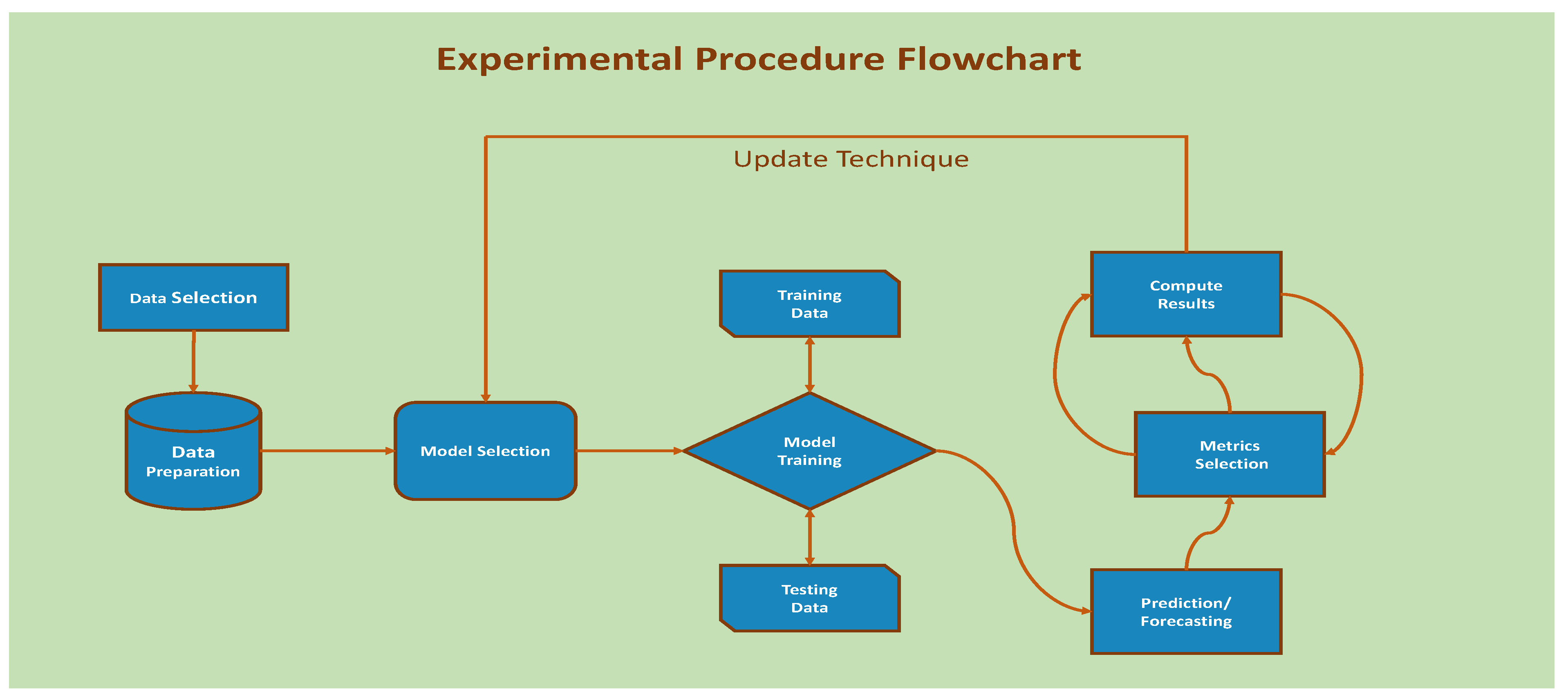
2.5. Experimental Procedure

This research work has gone through several experimental stages which have been visualized through the flowchart in Figure 1. Data selection and data preparation were performed in the first stages followed by the list of selected models chosen for this research work. Next, the data was trained after dividing into two portions; the training and testing portions. Following next, the critical step of prediction has been performed for each selected dataset and predictive model. Lastly, the performance of each model has been measured by all the selected evaluation criteria iteratively.

3. Results

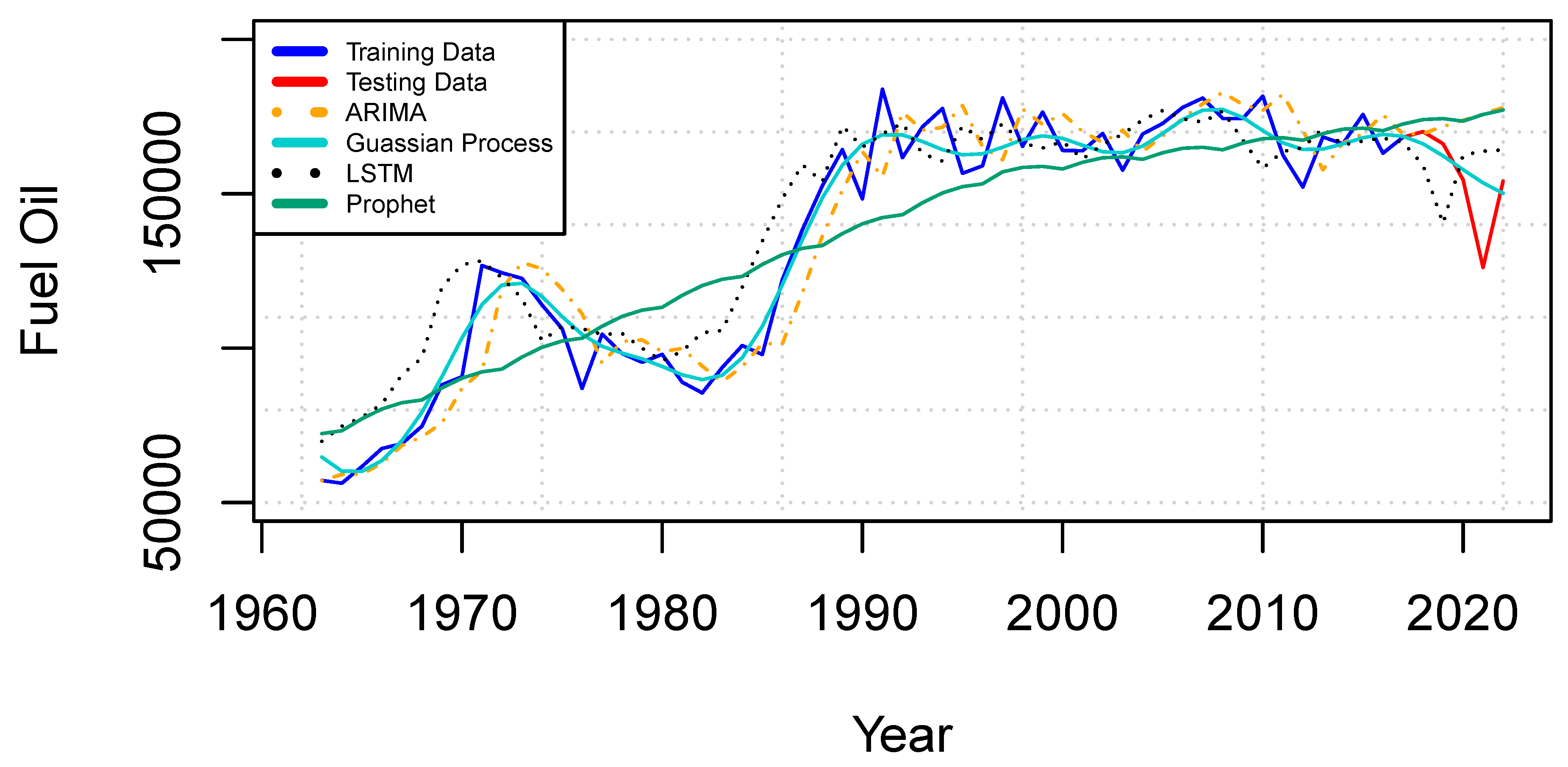
Table 2 highlights the selected model’s (Prophet, LSTM, GP, and ARIMA) performance for the fuel oil dataset using five evaluation metrics, including RMSE, MAPE, RAE, AIC, and Time consumption in seconds as described earlier. By looking at the presented results given below, the ARIMA model resulted in small forecasting errors for most of the evaluation criteria which are 18184.8, 12.4%, 0.42, 1158.9, and 0.7 for RMSE, MAPE%, RAE, AIC, and time consumption. Looking at RMSE, ARIMA produced an error of 13793.7, followed by LSTM 14564.1, and Prophet 18184.8, while GP resulted in 25052.6 as compared to all other forecasting techniques. The same performance was shown by the GP producing a greater value of 0.44 according to the evaluation metric RAE. considering MAPE, the ARIMA and GP models resulted in smaller forecasting error of of 7.7% and 4.8%. based on AIC, GP model produced smaller forecasting error of 1073.9 followed by LSTM, while the prophet produces a larger value of 1158.9. The time consumption or requirement for training the model indicated that ARIMA and GP models took less, i.e., 0.7 and 1.2 seconds, followed by Prophet while LSTM took more time approximately 128 seconds.

Figure 2, visualizes line trend plots for the selected forecasting models and trained as well as test values for the fuel oil dataset. The line plots show how well the model forecasts values by not only predicting values but also capturing the trend in the original values and forecasting values. The ARIMA and LSTM models have captured the trend comparatively well followed by GP which have also grasped the trend; however, more smoothness is available in the GP line. Looking at the line of the Prophet model, it looks narrower and straighter showing less efficiency in forecast.

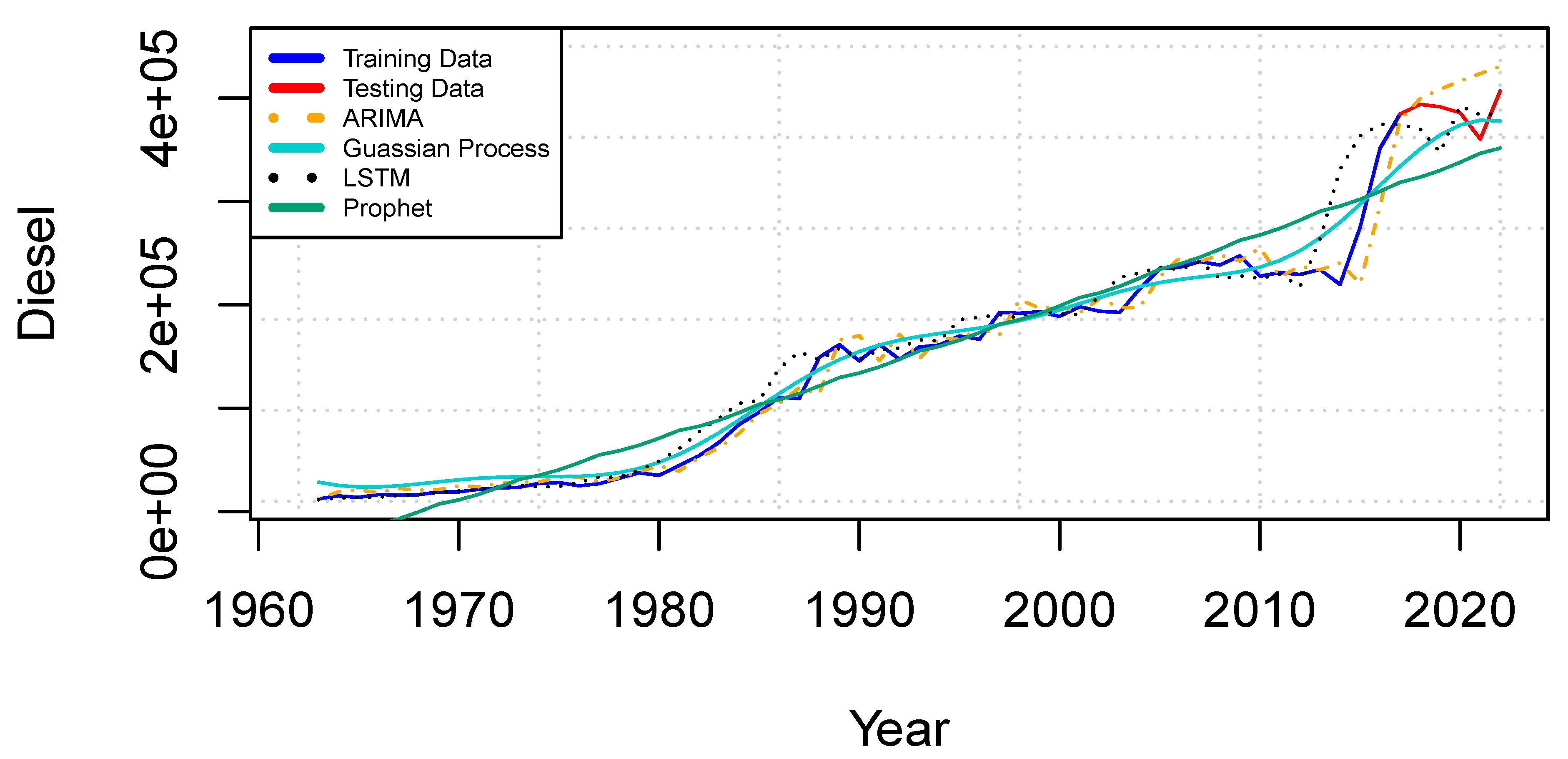
Table 3 displays the findings for the diesel dataset. For the majority of the evaluation metrics—RMSE, MAPE%, RAE, AIC, and training time—the ARIMA model demonstrated superior performance, achieving the lowest values: 17492.4 for RMSE, 10.7% for MAPE, 0.11 for RAE, 1175.1 for AIC, and 1 second for training time. Among all forecasting approaches, ARIMA produced the lowest RMSE value of 17492.4, followed closely by GP with 18133.1 and LSTM with 28952.5, whereas Prophet exhibited the highest RMSE at 29897.4. In terms of RAE, Prophet performed poorly with a higher value of 0.23, while ARIMA excelled with the lowest value of 0.11. For MAPE, both the LSTM and ARIMA models stood out, recording 16.1% and 10.7%, respectively. Regarding the AIC metric, the GP model achieved the lowest score at 1168.9, followed closely by ARIMA, while both Prophet and LSTM exceeded 1200. To assess the computational efficiency of the models, training time was also evaluated. The ARIMA and GP models demonstrated exceptional efficiency, completing training in just 0.8 and 1 second, respectively. Prophet followed with 2 seconds, while LSTM required significantly more time, exceeding 135 seconds. This metric highlights the importance of considering computational demands when selecting a forecasting method.

Figure 3 presents line trend charts for the selected forecasting models, along with the training and test values for the diesel dataset. Among these models, the LSTM and ARIMA plots exhibit the least deviation from the overall trend, indicating strong alignment. In contrast, the GP model’s test and training lines closely follow the observed trends, reflecting its effectiveness in capturing the dataset’s patterns.

A comparison between the Prophet model’s performance on the diesel dataset and its results on the fuel oil dataset reveals a notable difference: the diesel dataset’s trend line aligns more closely with the training and test lines, highlighting improved forecasting consistency.

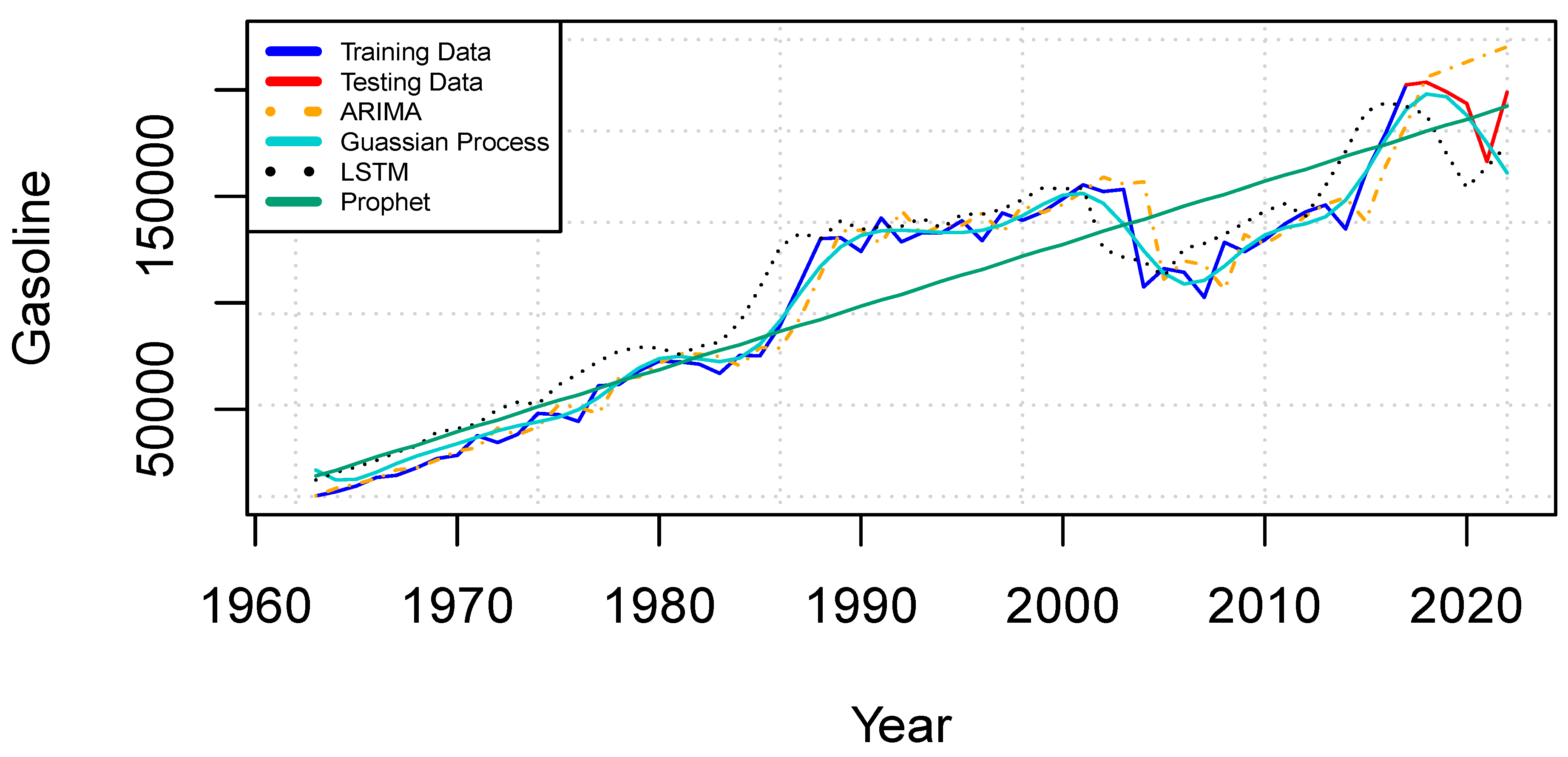
The results for the gasoline dataset are summarized in Table 4. The GP model outperformed others in most evaluation metrics, including time consumption, RMSE, MAPE%, RAE, and AIC, with values of 0.7 seconds, 7893.6, 9.3%, 0.11, and 1065.4, respectively. Among all forecasting techniques, the LSTM model exhibited the highest RMSE at 20635.8, while the GP model achieved the lowest RMSE of 7893.6, followed by ARIMA with 13024.4 and Prophet with 19919.8. Similarly, the RAE metric showed LSTM with the highest score of 0.38, whereas the GP model reported the smallest value, indicating superior performance. For MAPE, the GP and ARIMA models achieved the lowest predictions at 9.3% and 8.2%, respectively. In terms of the AIC metric, the GP model again delivered the most favorable value of 1065.4, followed by ARIMA at 1139.5, while Prophet and LSTM recorded higher values of 1183.3 and 1153.4, respectively.

To evaluate computational efficiency, training time was used as the fifth metric. The ARIMA and GP models demonstrated exceptional speed, completing forecasting in 1 and 0.7 seconds, respectively. Prophet required 2 seconds, while the LSTM model demanded significantly more time, exceeding 121 seconds. These results highlight the GP model’s ability to balance accuracy and efficiency effectively across various evaluation criteria.

Figure 4 illustrates the line trend charts for the selected forecasting models, alongside the training and test values for the gasoline dataset. Once again, the GP model demonstrates a strong ability to capture the overall trend, with its test and training lines closely aligned to the data pattern. In contrast, the LSTM and ARIMA models manage to follow the minimal trend effectively but exhibit less precision compared to GP. For the gasoline dataset, the Prophet model generates a straight line, reflecting its limitations in capturing the dataset’s variations.

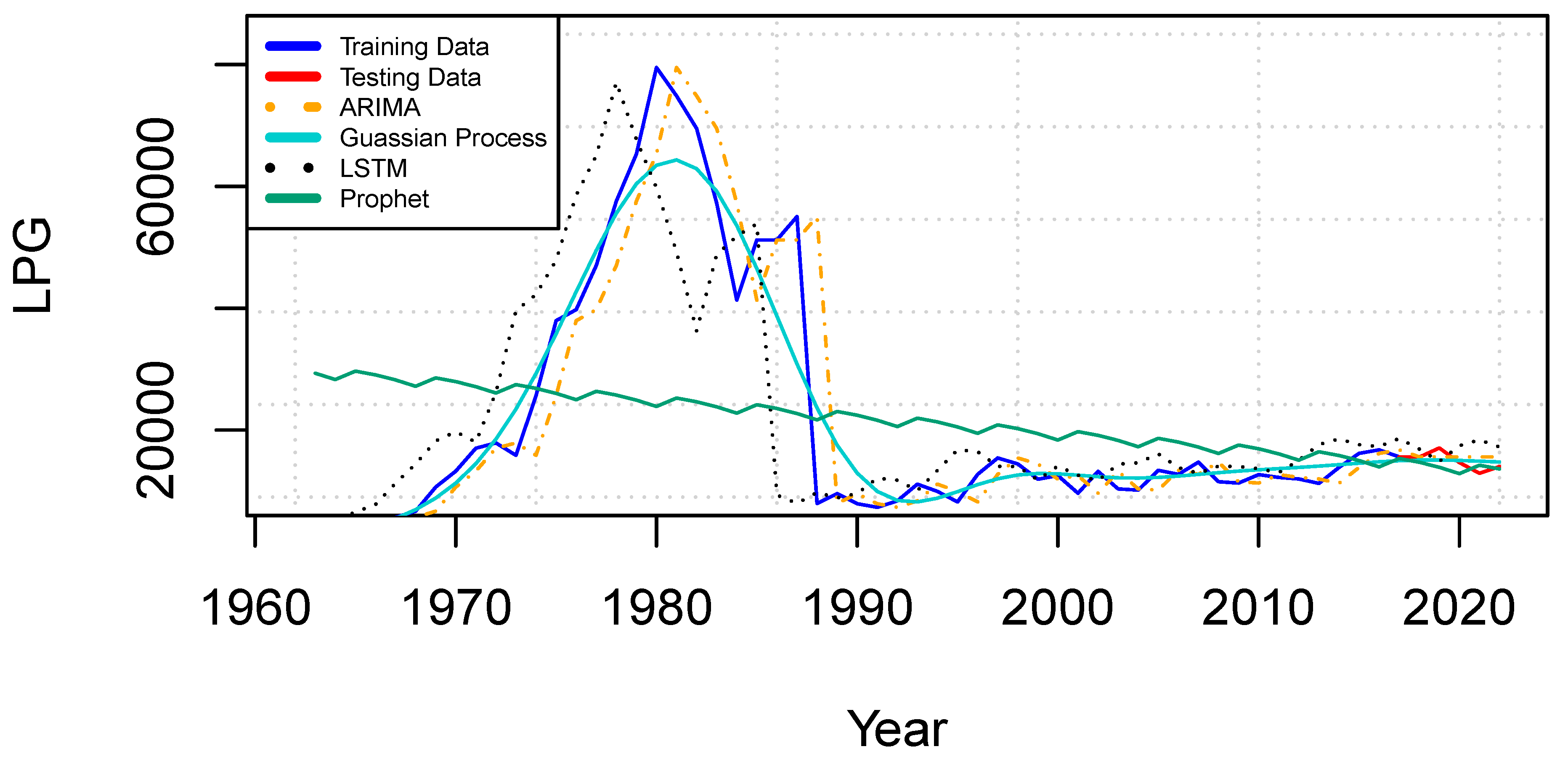
The results for the LPG dataset, presented in Table 5, highlight the performance of the forecasting models across various evaluation metrics. The GP model achieved the lowest values for most criteria, including time consumption, RMSE, MAPE%, RAE, and AIC, with values of 1 second, 5318.8, 19.2%, 0.19, and 1019.3, respectively. In contrast, the Prophet model recorded the highest RMSE at 18950.5, while the GP model achieved the lowest RMSE at 5318.8, followed by ARIMA at 7799.5 and LSTM at 12467.8. The Prophet model also exhibited the highest RAE at 0.92, while the GP model delivered the smallest RAE value of 0.19. For MAPE, the GP and ARIMA models performed well with predictions of 19.2% and 25.8%, respectively, while the Prophet model produced a significantly higher MAPE of 152.8%. Regarding AIC, Prophet and LSTM predicted lower values at 1017.2 and 1118.8, while ARIMA and GP reported slightly higher values of 1077.3 and 1019.3. Training time was also a crucial factor in evaluating the models. Similar to other datasets, ARIMA, Prophet, and GP demonstrated exceptional efficiency, completing forecasting in just 1 second, whereas LSTM required approximately 112 seconds to train.

Figure 5 illustrates a comparative analysis of the forecasting models for the LPG dataset. The LSTM and ARIMA models demonstrate strong performance by closely tracking the actual values and effectively capturing the underlying trend. The GP model also performs well, generating a smooth curve that aligns reasonably with the observed data. However, the Prophet model continues to show limitations, producing an almost straight-line prediction that fails to capture the dynamic variations of the data set.

Table 6 presents the results for the Kerosene Aviation Fuels dataset. Among the evaluation criteria—time consumption, RMSE, MAPE%, RAE, and AIC—the GP model consistently predicted the lowest values, with results of 1 second for training time, 6628.5 for RMSE, 11.1% for MAPE, 0.18 for RAE, and 1045.5 for AIC. In contrast, the LSTM model yielded the highest RMSE value of 12163.3, surpassing all other forecasting methods. The GP model again excelled, predicting the lowest RMSE at 6628.5, followed by ARIMA at 10137.5 and Prophet at 11581.5. For the RAE metric, the GP model achieved the lowest value of 0.18, followed by ARIMA at 0.22, while the Prophet model once again exhibited the highest value at 37.8%. When examining AIC and training time, ARIMA and GP models again stood out with the most efficient performance, both in terms of lower AIC values and faster training times. This trend is further illustrated in Figure 6, where the performance of all models, much like the previous dataset, shows consistent results in terms of trend alignment and smoothness.

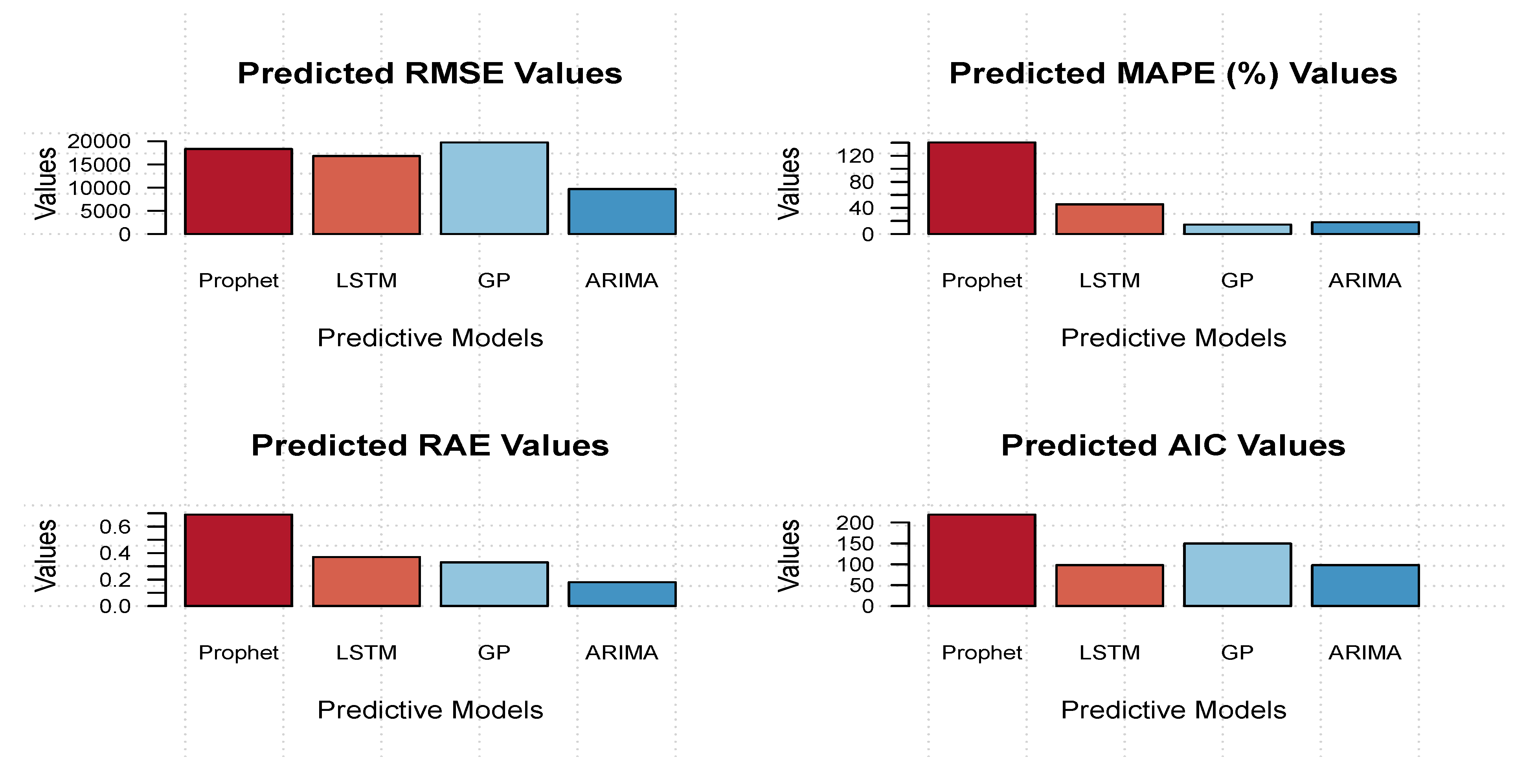
To summarize the performance of the selected models across multiple datasets and evaluation metrics, we present a bar graph in Figure 7 that visualizes the predicted values for RMSE, MAPE, RAE, and AIC. This graph allows us to assess the overall performance of each model, where smaller values indicate better performance across all datasets. As discussed in detail in previous sections, the Prophet model consistently yielded higher values for all metrics and datasets, making it the least effective overall.

In contrast, the LSTM and GP models showed mixed results, with performance varying from smaller to larger values depending on the dataset and metric. However, the ARIMA model consistently delivered lower values across all datasets and evaluation criteria, demonstrating stable performance. Furthermore, LSTM and ARIMA were the only models to closely follow the trend of the actual values, with ARIMA showing a smoother fit. The Prophet model, while following the general trend, failed to capture the underlying data pattern effectively, producing predictions that were closer to the actual values but lacked trend accuracy.

4. Discussion

This study presents a detailed comparison of four forecasting models - ARIMA, LSTM, GP and Prophet - applied to predict refined petroleum production in Saudi Arabia using several data sets: gasoline, LPG, aviation fuels kerosene and fuel oil. The goal was to assess the precision, computational efficiency and practical applicability of these models in forecasting petroleum production data over a period that spanned from 1962 to 2022. A set of evaluation metrics including RMSE (Root Mean Squared Error), MAPE (Mean Absolute Percentage Error), RAE (Relative Absolute Error), AIC (Akaike Information Criterion) and training time were used to analyse the model performance. Across all data sets, gasoline, LPG and Kerosene Aviation Fuels, the Gaussian Process (GP) model consistently demonstrated superior performance in terms of both forecast accuracy and computational efficiency. In the gasoline dataset, GP achieved the lowest RMSE of 7893.6, the lowest MAPE of 9.3%, and the lowest RAE of 0.11, completing training in just 0.7 seconds. These results highlight the model’s strong capability in capturing complex non-linear relationships within the data. A similar pattern of out performance was observed for the LPG dataset, where GP recorded the lowest RMSE of 5318.8, MAPE of 19.2%, and RAE of 0.19, again demonstrating the robustness of the model. For Kerosene Aviation Fuels, GP maintained its lead with the lowest RMSE of 6628.5, MAPE of 11. 1% and RAE of 0.18, continuing to show its ability to accurately predict refined petroleum production while being computationally efficient, completing training in 1 second for most datasets. This makes the GP model the most reliable and efficient option for forecasting petroleum production data across all scenarios.

The ARIMA model, though not as effective as GP in terms of accuracy, still showed strong performance across all datasets. ARIMA demonstrated stable results with moderate RMSE and MAPE values and relatively low RAE scores, indicating that it was able to capture the general trend in the data. For example, in the gasoline dataset, ARIMA produced an RMSE of 13024.4 and MAPE of 8.2%, while in the LPG dataset, it recorded RMSE of 7799.5 and MAPE of 25.8%, both outperforming the Prophet and LSTM models. One of the major advantages of ARIMA is its computational efficiency; it achieved a training time as low as 1 second across all datasets, which is particularly valuable when dealing with large datasets or real-time forecasting needs. The moderate accuracy of ARIMA and the fast training time make it a suitable choice for applications where speed is essential, and the data patterns are relatively stable and less complex.

The LSTM (Long Short-Term Memory) model showed promise in terms of its ability to capture complex relationships in the data but struggled with consistent performance across datasets. For example, in the gasoline dataset, LSTM produced the highest RMSE of 20635.8 and the RAE of 0.38, indicating that it struggled to achieve the same level of accuracy as GP and ARIMA. This discrepancy highlights that LSTM is not always the best choice for petroleum production forecasting, especially when the data do not exhibit strong nonlinear patterns or when there is a lack of sufficient data. Furthermore, LSTM required significantly longer training times compared to the other models, with training times exceeding 121 seconds for most datasets, making it computationally expensive. This makes LSTM less ideal for real-time forecasting applications where speed is a priority. Despite its potential to model nonlinear relationships, its performance was hindered by overfitting and the large amount of training data required to achieve good results.

The Prophet model, which is often considered for its ability to handle seasonality, was the least effective among the models in this study. Despite its strengths in modeling seasonal data, Prophet struggled to capture the complex and non-linear trends present in the petroleum production datasets. For example, in the gasoline dataset, Prophet achieved an RMSE of 19919.8 and MAPE of 41.1%, while in the LPG dataset, it recorded an RMSE of 18950.5 and MAPE of 152% - the highest among all models. These high error values indicate Prophet’s failure to accurately capture the underlying patterns in the data. The model produced overly linear forecasts that could not reflect the dynamic nature of the petroleum production data. In addition to poor accuracy, Prophet also exhibited relatively slow training times, taking up to 2 seconds for most datasets, which is still slower than ARIMA and GP, although faster than LSTM. These results underline Prophet’s limitations when applied to complex nonlinear forecasting tasks like petroleum production.

A critical aspect of this study was the assessment of the computational efficiency of each model, particularly in real-time forecasting applications. Both GP and ARIMA demonstrated impressive training times, completing training in less than 2 seconds for all datasets, with ARIMA being the fastest at 1 second. This makes ARIMA and GP highly suitable for practical, large-scale forecasting tasks where quick decision-making is essential. In contrast, the LSTM model, due to its deep learning nature, was computationally expensive, with training times frequently exceeding 120 seconds for most datasets. This long training time makes LSTM unsuitable for real-time applications. Prophet, while not as slow as LSTM, still lagged behind ARIMA and GP, with training times averaging around 2 seconds, which is slower than ARIMA but still reasonably fast.

5. Conclusions

This study, conducted a comprehensive evaluation of predictive modeling techniques to estimate the output of refined petroleum products in Saudi Arabia. Both time series and machine learning approaches for forecasting are used in this study. We explored a variety of machine learning models, including the Gaussian Process (GP), Facebook Prophet, Long Short-Term Memory (LSTM), and Auto-Regressive Integrated Moving Average (ARIMA). Each model was rigorously evaluated based on its ability to forecast refined petroleum output using historical data from 1962 to 2022. To assess model performance, we employed several key metrics, including Root Mean Squared Error (RMSE), Mean Absolute Percentage Error (MAPE), Relative Absolute Error (RAE), Akaike Information Criterion (AIC), and training time.

Our findings revealed subtle performance differences across the models and datasets. Notably, the ARIMA model demonstrated consistent robustness in capturing the underlying patterns in refined petroleum output, with superior forecasting accuracy across multiple metrics for most datasets. In contrast, the Prophet model was less reliable, often yielding higher error metrics and failing to capture the complex patterns within the data.

In the future, several research directions can be pursued. Exogenous factors can be added to the models to improve their prediction power and offer a deeper understanding of the dynamics of refined petroleum production. Furthermore, one can investigating ensemble modeling strategies that integrate many models.

References

- Ceylan, H.; Ozturk, H.K. Estimating energy demand of Turkey based on economic indicators using genetic algorithm approach. Energy Conversion and Management 2004, 45, 2525–2537. [Google Scholar] [CrossRef]
- Kontopoulou, V.I.; et al. A review of ARIMA vs. machine learning approaches for time series forecasting in data driven networks. Future Internet 2023, 15, 255. [Google Scholar] [CrossRef]
- Santangelo, O.E.; et al. Machine learning and prediction of infectious diseases: a systematic review. Machine Learning and Knowledge Extraction 2023, 5, 175–198. [Google Scholar] [CrossRef]
- Ilu, S.Y.; Prasad, R. Improved autoregressive integrated moving average model for COVID-19 prediction by using statistical significance and clustering techniques. Heliyon 2023, 9. [Google Scholar] [CrossRef] [PubMed]
- Álvarez-Chaves, H.; Muñoz, P.; R-Moreno, M.D. Machine learning methods for predicting the admissions and hospitalisations in the emergency department of a civil and military hospital. Journal of Intelligent Information Systems 2023, 61, 881–900. [Google Scholar] [CrossRef]
- Ansari, M.; Alam, M. An intelligent IoT-cloud-based air pollution forecasting model using univariate time-series analysis. Arabian Journal for Science and Engineering 2023, 1–28. [Google Scholar] [CrossRef]
- Parlak, F. The forecast performances of the classical time series model and machine learning algorithms on BIST-50 price index using exogenous variables. MS thesis, Middle East Technical University, 2023. [Google Scholar]
- Murugesan, R.; Mishra, E.; Krishnan, A.H. Deep learning based models: Basic LSTM, Bi LSTM, Stacked LSTM, CNN LSTM and Conv LSTM to forecast agricultural commodities prices. Preprint 2021. [Google Scholar]
- Feng, T.; Zheng, Z.; Yu, X. The comparative analysis of SARIMA, Facebook Prophet, and LSTM for road traffic injury prediction in Northeast China. Frontiers in Public Health 2022, 10, 946563. [Google Scholar] [CrossRef]
- Suganthi, L.; Samuel, A.A. Energy models for demand forecasting—A review. Renewable and Sustainable Energy Reviews 2012, 16, 1223–1240. [Google Scholar] [CrossRef]
- Ekonomou, L. Greek long-term energy consumption prediction using artificial neural networks. Energy 2010, 35, 512–517. [Google Scholar] [CrossRef]
- Guarnaccia, C.; et al. Development of seasonal ARIMA models for traffic noise forecasting. MATEC Web of Conferences, EDP Sciences 2017, 125. [Google Scholar] [CrossRef]
- Theerthagiri, P.; Ruby, A.U. Seasonal learning based ARIMA algorithm for prediction of Brent oil Price trends. Multimedia Tools and Applications 2023, 82, 24485–24504. [Google Scholar] [CrossRef]
- Grigoraș, A.; Leon, F. Transformer-Based Model for Predicting Customers’ Next Purchase Day in e-Commerce. Computation 2023, 11, 210. [Google Scholar] [CrossRef]
- Contreras, J.; et al. ARIMA models to predict next-day electricity prices. IEEE Transactions on Power Systems 2003, 18, 1014–1020. [Google Scholar] [CrossRef]
- Agrawal, R.K.; Muchahary, F.; Tripathi, M.M. Long term load forecasting with hourly predictions based on long-short-term-memory networks. In Proceedings of the 2018 IEEE Texas Power and Energy Conference (TPEC); IEEE, 2018. [Google Scholar]
- Telo, J. Web traffic prediction using Autoregressive, LSTM, and XGBoost time series models. Applied Research in Artificial Intelligence and Cloud Computing 2020, 3, 1–15. [Google Scholar]
- Gupta, R.; et al. Time series forecasting of solar power generation using Facebook prophet and XG boost. In Proceedings of the 2022 IEEE Delhi Section Conference (DELCON); IEEE, 2022. [Google Scholar]
- Ganapathy, G.P.; et al. Rainfall forecasting using machine learning algorithms for localized events. Comput. Mater. Contin. 2022, 71, 6333–6350. [Google Scholar]
- Othman, K.M.; et al. Evaluating and Comparing the Performance of Statistical and Artificial Intelligence Algorithms to Achieve Improved Load Forecasting in Saudi Arabia. Available at SSRN: https://ssrn.com/abstract=4484535.
- Natarajan, Y.; et al. Enhancing Building Energy Efficiency with IoT-Driven Hybrid Deep Learning Models for Accurate Energy Consumption Prediction. Sustainability 2024, 16, 1925. [Google Scholar] [CrossRef]
- Soto-Ferrari, M.; Carrasco-Pena, A.; Prieto, D. Deep Learning Architectures Framework for Emerging Outbreak Forecasting of Mpox: A Bagged Ensemble Scheme to Model Accurate Prediction Intervals. 2023. [Google Scholar]
- Niyogi, D.; Srinivasan, J. Accurate Prediction of Global Mean Temperature through Data Transformation Techniques. arXiv preprint 2023, arXiv:2303.06468. [Google Scholar]
- Jahin, M.A.; et al. Big Data-Supply Chain Management Framework for Forecasting: Data Preprocessing and Machine Learning Techniques. arXiv preprint 2023, arXiv:2307.12971. [Google Scholar]
- Zhang, J.; Yang, Y.; Feng, Y. Hybrid Time-Series Prediction Method Based on Entropy Fusion Feature. International Journal of Intelligent Systems 2023, 2023. [Google Scholar] [CrossRef]
- Kożuch, A.; Cywicka, D.; Adamowicz, K. A comparison of artificial neural network and time series models for timber price forecasting. Forests 2023, 14, 177. [Google Scholar] [CrossRef]
- Mandalis, P.; et al. Towards a Unified Vessel Traffic Flow Forecasting Framework. In Proceedings of the EDBT/ICDT Workshops; 2023. [Google Scholar]
- Zhao, J.; et al. A Novel Short-Time Passenger Flow Prediction Method for Urban Rail Transit: CEEMDAN-CSSA-LSTM Model Based on Station Classification. Engineering Letters 2023, 31. [Google Scholar]
- Shin, S.-Y.; Woo, H.-G. Energy consumption forecasting in Korea using machine learning algorithms. Energies 2022, 15, 4880. [Google Scholar] [CrossRef]
- Wang, H.; Chen, S. Insights into the Application of Machine Learning in Reservoir Engineering: Current Developments and Future Trends. Energies 2023, 16, 1392. [Google Scholar] [CrossRef]
- Dudek, G.; Piotrowski, P.; Baczyński, D. Intelligent Forecasting and Optimization in Electrical Power Systems: Advances in Models and Applications. Energies 2023, 16, 3024. [Google Scholar] [CrossRef]
- Saglam, M.; Spataru, C.; Karaman, O.A. Forecasting electricity demand in Turkey using optimization and machine learning algorithms. Energies 2023, 16, 4499. [Google Scholar] [CrossRef]
- Çodur, M.K. Ensemble Machine Learning Approaches for Prediction of Türkiye’s Energy Demand. 2023. [Google Scholar]
- Paassen, B.; Göpfert, C.; Hammer, B. Gaussian process prediction for time series of structured data. In Proceedings of the ESANN; 2016. [Google Scholar]
- Al-Rakhami, M.; et al. An ensemble learning approach for accurate energy load prediction in residential buildings. IEEE Access 2019, 7, 48328–48338. [Google Scholar] [CrossRef]
- Alali, Y.; Harrou, F.; Sun, Y. A proficient approach to forecast COVID-19 spread via optimized dynamic machine learning models. Sci. Rep. 2022, 12, 2467. [Google Scholar] [CrossRef]
- Kumar, S.V.; Vanajakshi, L. Short-term traffic flow prediction using seasonal ARIMA model with limited input data. European Transport Research Review 2015, 7, 1–9. [Google Scholar] [CrossRef]
- Nespoli, A.; et al. Day-ahead photovoltaic forecasting: A comparison of the most effective techniques. Energies 2019, 12, 1621. [Google Scholar] [CrossRef]
- Chadalavada, R.J.; Raghavendra, S.; Rekha, V. Electricity requirement prediction using time series and Facebook’s PROPHET. Indian J. Sci. Technol. 2020, 13, 4631–4645. [Google Scholar] [CrossRef]
- Taylor, S. J.; Letham, B. Forecasting at scale. The American Statistician 2018, 72, 37–45. [Google Scholar] [CrossRef]
- Ahmad, F.; Finos, L.; Guidolin, M. Forecasting hydropower with innovation diffusion models: A cross-country analysis. Forecasting 2024, 6, 1045–1064. [Google Scholar] [CrossRef]
- Jarrah, M.; Derbali, M. Predicting Saudi Stock Market Index by Using Multivariate Time Series Based on Deep Learning. Applied Sciences 2023, 13, 8356. [Google Scholar] [CrossRef]
- Herrera, G.P.; et al. Long-term forecast of energy commodities price using machine learning. Energy 2019, 179, 214–221. [Google Scholar] [CrossRef]
- Liu, T.; et al. Industrial time series forecasting based on improved Gaussian process regression. Soft Computing 2020, 24, 15853–15869. [Google Scholar] [CrossRef]
- Han, J.; Lin, H.; Qin, Z. Prediction and Comparison of In-Vehicle CO2 Concentration Based on ARIMA and LSTM Models. Applied Sciences 2023, 13, 10858. [Google Scholar] [CrossRef]
- Zhu, Q.; Guo, Y.; Feng, G. Household energy consumption in China: Forecasting with BVAR model up to 2015. In Proceedings of the 2012 Fifth International Joint Conference on Computational Sciences and Optimization; IEEE, 2012. [Google Scholar]
- Waseem, K.H.; et al. Forecasting of air quality using an optimized recurrent neural network. Processes 2022, 10, 2117. [Google Scholar] [CrossRef]