
Submitted:
20 November 2024
Posted:
21 November 2024
You are already at the latest version
Abstract
Determining the values of various properties for new bioinks for 3D printing is a very important task in the design of new materials. For this purpose, a large number of experimental works have been consulted and a database with >1200 bioprinting tests has been created. These tests cover different combinations of conditions in terms of print pressure, temperature, and needle values, for example. These data are difficult to deal with in terms of determining combinations of conditions to optimize the tests and to analyze new options. The best model presented has values of specificity = Sp (%) = 88.4, sensitivity = Sn (%) = 86.2 in training series and Sp (%) = 85.9, Sn (%) = 80.3 in external validation series. This model uses operators based on perturbation theory in order to analyze the complexity of the data. The performance of the model has been compared with neural networks with very similar results. This tool could be easily applied to predict the properties of in silico bioprinting assays.
Keywords:
1. Introduction
2. Materials and Methods
2.1. Computational Methods
2.1.1. Database Creation
2.1.2. Descriptors Calculation
2.1.3. Outcome Classification
2.1.4. Model Generation Process
3. Experimental Methods
3.1. Bioprinting Conditions
3.2. Image Caption and Analysis
4. Results and Discussion
4.1. Computational Model
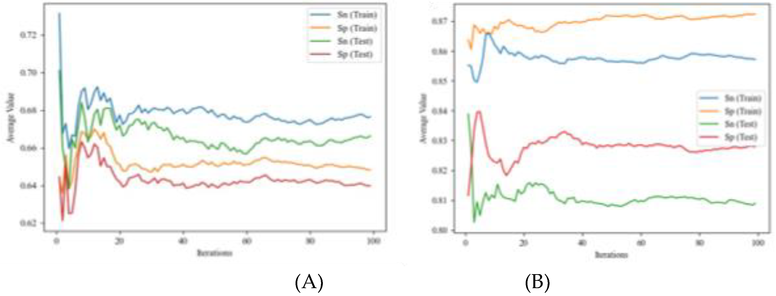
4.1.1. IFPTML Linear Model
4.1.2. IFPTML Non-Linear Models

| Profile | Training | Validation | ||||||
|---|---|---|---|---|---|---|---|---|
| f(vi,j) | 0a | 1a | (%) | Par. | (%) | 0a | 1a | |
| IFPTML-MLPC 1:1-100-100-1:1 |
0b | 352 | 222 | 77.4 | Sp | 56.8 | 134 | 102 |
| 1b | 118 | 405 | 61.3 | Sn | 77.4 | 53 | 182 | |
| AUROC | 0.694 | 0.671 | ||||||
| IFPTML-MLPC 1:1-100-100-100-1:1 |
0b | 491 | 83 | 85.5 | Sp | 78.8 | 186 | 50 |
| 1b | 170 | 353 | 67.5 | Sn | 63.8 | 85 | 750 | |
| AUROC | 0.765 | 0.713 | ||||||
| IFPTML-MLPC 1:1-100-1100-100-1:1 |
0b | 187 | 82 | 85.7 | Sp | 79.2 | 187 | 49 |
| 1b | 171 | 352 | 67.3 | Sn | 63.0 | 87 | 148 | |
| AUROC | 0.765 | 0.711 | ||||||
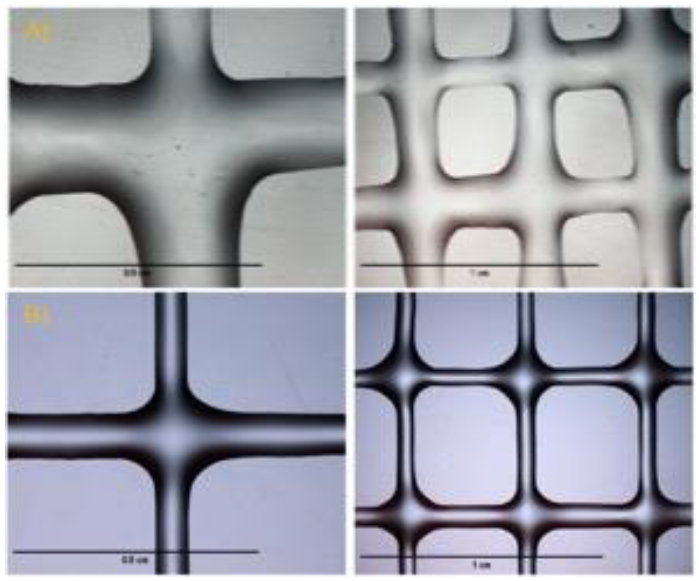
4.2. Experimental and Computational Case of Study of ChiMA Gel
4.2.1. Experimental Characterization of Two New ChiMA and ChiMA + PEGDA Hydrogel
4.2.2. IFPTML Computational Simulation of ChiMA Gel
5. Conclusions
Author Contributions
Funding
Data Availability Statement
Conflicts of Interest
References
- Roche, C.D.; Brereton, R.J.L.; Ashton, A.W.; Jackson, C.; Gentile, C. Current challenges in three-dimensional bioprinting heart tissues for cardiac surgery. European Journal of Cardio-Thoracic Surgery 2020, 58, 500–510. [Google Scholar] [CrossRef] [PubMed]
- Unagolla, J.M.; Jayasuriya, A.C. Hydrogel-based 3D bioprinting: A comprehensive review on cell-laden hydrogels, bioink formulations, and future perspectives. Applied Materials Today 2020, 18, 100479. [Google Scholar] [CrossRef] [PubMed]
- Chimene, D.; Lennox, K.K.; Kaunas, R.R.; Gaharwar, A.K. Advanced Bioinks for 3D Printing: A Materials Science Perspective. Annals of Biomedical Engineering 2016, 44, 2090–2102. [Google Scholar] [CrossRef] [PubMed]
- Shah, P.P.; Shah, H.B.; Maniar, K.K.; Özel, T. Extrusion-based 3D bioprinting of alginate-based tissue constructs. Procedia CIRP 2020, 95, 143–148. [Google Scholar] [CrossRef]
- Huang, J.; Lei, X.; Huang, Z.; Rong, Z.; Li, H.; Xie, Y.; Duan, L.; Xiong, J.; Wang, D.; Zhu, S.; et al. Bioprinted Gelatin-Recombinant Type III Collagen Hydrogel Promotes Wound Healing. Int J Bioprint 2022, 8, 517. [Google Scholar] [CrossRef] [PubMed]
- Ding, Y.-W.; Zhang, X.-W.; Mi, C.-H.; Qi, X.-Y.; Zhou, J.; Wei, D.-X. Recent advances in hyaluronic acid-based hydrogels for 3D bioprinting in tissue engineering applications. Smart Materials in Medicine 2023, 4, 59–68. [Google Scholar] [CrossRef]
- Piluso, S.; Skvortsov, G.A.; Altunbek, M.; Afghah, F.; Khani, N.; Koç, B.; Patterson, J. 3D bioprinting of molecularly engineered PEG-based hydrogels utilizing gelatin fragments. Biofabrication 2021, 13. [Google Scholar] [CrossRef]
- Rosińska, K.; Bartniak, M.; Wierzbicka, A.; Sobczyk-Guzenda, A.; Bociaga, D. Solvent types used for the preparation of hydrogels determine their mechanical properties and influence cell viability through gelatine and calcium ions release. J Biomed Mater Res B Appl Biomater 2023, 111, 314–330. [Google Scholar] [CrossRef]
- Darmau, B.; Hoang, A.; Gross, A.J.; Texier, I. Water-based synthesis of dextran-methacrylate and its use to design hydrogels for biomedical applications. European Polymer Journal 2024, 221, 113515. [Google Scholar] [CrossRef]
- Shamma, R.N.; Sayed, R.H.; Madry, H.; El Sayed, N.S.; Cucchiarini, M. Triblock Copolymer Bioinks in Hydrogel Three-Dimensional Printing for Regenerative Medicine: A Focus on Pluronic F127. Tissue Engineering Part B: Reviews 2021, 28, 451–463. [Google Scholar] [CrossRef]
- Wang, M.; Bai, J.; Shao, K.; Tang, W.; Zhao, X.; Lin, D.; Huang, S.; Chen, C.; Ding, Z.; Ye, J. Poly(vinyl alcohol) Hydrogels: The Old and New Functional Materials. International Journal of Polymer Science 2021, 2021, 2225426. [Google Scholar] [CrossRef]
- Ye, J.; Qian, C.; Dong, Y.; Zhu, Y.; Fu, Y. Development of organic solvent-induced shape memory poly(ethylene-co-vinyl acetate) monoliths for expandable oil absorbers. European Polymer Journal 2023, 183, 111730. [Google Scholar] [CrossRef]
- Dwivedi, R.; Kumar, S.; Pandey, R.; Mahajan, A.; Nandana, D.; Katti, D.S.; Mehrotra, D. Polycaprolactone as biomaterial for bone scaffolds: Review of literature. J Oral Biol Craniofac Res 2020, 10, 381–388. [Google Scholar] [CrossRef] [PubMed]
- Rodríguez-Rego, J.M.; Mendoza-Cerezo, L.; Macías-García, A.; Mendoza-Cerezo, L.; Carrasco-Amador, J.P.; Marcos-Romero, A.C. Methodology for characterizing the printability of hydrogels. Int J Bioprint 2023, 9, 667. [Google Scholar] [CrossRef] [PubMed]
- Dell, A.C.; Wagner, G.; Own, J.; Geibel, J.P. 3D Bioprinting Using Hydrogels: Cell Inks and Tissue Engineering Applications. Pharmaceutics 2022, 14. [Google Scholar] [CrossRef] [PubMed]
- Kaliaraj, G.S.; Shanmugam, D.K.; Dasan, A.; Mosas, K.K. Hydrogels—A Promising Materials for 3D Printing Technology. Gels 2023, 9. [Google Scholar] [CrossRef]
- Martin, T.B.; Audus, D.J. Emerging Trends in Machine Learning: A Polymer Perspective. ACS Polymers Au 2023, 3, 239–258. [Google Scholar] [CrossRef]
- Naghieh, S.; Chen, X. Printability–A key issue in extrusion-based bioprinting. Journal of Pharmaceutical Analysis 2021, 11, 564–579. [Google Scholar] [CrossRef]
- Zhang, T.; Zhao, W.; Zijie, X.H.; Wang, X.W.; Zhang, K.X.; Yin, J.B. Bioink design for extrusion-based bioprinting. APPLIED MATERIALS TODAY 2021, 25. [Google Scholar] [CrossRef]
- He, Y.; Yang, F.; Zhao, H.; Gao, Q.; Xia, B.; Fu, J. Research on the printability of hydrogels in 3D bioprinting. Scientific Reports 2016, 6, 29977. [Google Scholar] [CrossRef]
- Lai, J.; Ye, X.; Liu, J.; Wang, C.; Li, J.; Wang, X.; Ma, M.; Wang, M. 4D printing of highly printable and shape morphing hydrogels composed of alginate and methylcellulose. Materials & Design 2021, 205, 109699. [Google Scholar] [CrossRef]
- Jin, W.; Liu, H.; Li, Z.; Nie, P.; Zhao, G.; Cheng, X.; Zheng, G.; Yang, X. Effect of Hydrogel Contact Angle on Wall Thickness of Artificial Blood Vessel. International Journal of Molecular Sciences 2022, 23. [Google Scholar] [CrossRef] [PubMed]
- Mancha Sánchez, E.; Gómez-Blanco, J.C.; López Nieto, E.; Casado, J.G.; Macías-García, A.; Díaz Díez, M.A.; Carrasco-Amador, J.P.; Torrejón Martín, D.; Sánchez-Margallo, F.M.; Pagador, J.B. Hydrogels for Bioprinting: A Systematic Review of Hydrogels Synthesis, Bioprinting Parameters, and Bioprinted Structures Behavior. Frontiers in Bioengineering and Biotechnology 2020, 8. [Google Scholar] [CrossRef] [PubMed]
- Sällström, N.; Goulas, A.; Martin, S.; Engstrøm, D.S. The effect of print speed and material aging on the mechanical properties of a self-healing nanocomposite hydrogel. Additive Manufacturing 2020, 35, 101253. [Google Scholar] [CrossRef]
- Strauß, S.; Schroth, B.; Hubbuch, J. Evaluation of the Reproducibility and Robustness of Extrusion-Based Bioprinting Processes Applying a Flow Sensor. Front Bioeng Biotechnol 2022, 10, 831350. [Google Scholar] [CrossRef] [PubMed]
- Lee, U.N.; Day, J.H.; Haack, A.J.; Bretherton, R.C.; Lu, W.; DeForest, C.A.; Theberge, A.B.; Berthier, E. Layer-by-layer fabrication of 3D hydrogel structures using open microfluidics. Lab Chip 2020, 20, 525–536. [Google Scholar] [CrossRef]
- Göhl, J.; Markstedt, K.; Mark, A.; Håkansson, K.; Gatenholm, P.; Edelvik, F. Simulations of 3D bioprinting: Predicting bioprintability of nanofibrillar inks. Biofabrication 2018, 10, 034105. [Google Scholar] [CrossRef]
- GhavamiNejad, A.; Ashammakhi, N.; Wu, X.Y.; Khademhosseini, A. Crosslinking Strategies for 3D Bioprinting of Polymeric Hydrogels. Small 2020, 16, 2002931. [Google Scholar] [CrossRef]
- Xie, S. Perspectives on development of biomedical polymer materials in artificial intelligence age. Journal of Biomaterials Applications 2023, 37, 1355–1375. [Google Scholar] [CrossRef]
- Hulsen, T. Literature analysis of artificial intelligence in biomedicine. Ann Transl Med 2022, 10, 1284. [Google Scholar] [CrossRef]
- Mazón-Ortiz, G.; Cerda-Mejía, G.; Gutiérrez Morales, E.; Diéguez-Santana, K.; Ruso, J.M.; González-Díaz, H. Trends in Nanoparticles for Leishmania Treatment: A Bibliometric and Network Analysis. Diseases 2023, 11. [Google Scholar] [CrossRef] [PubMed]
- Nocedo-Mena, D.; Cornelio, C.; Camacho-Corona, M.D.R.; Garza-González, E.; Waksman de Torres, N.; Arrasate, S.; Sotomayor, N.; Lete, E.; González-Díaz, H. Modeling Antibacterial Activity with Machine Learning and Fusion of Chemical Structure Information with Microorganism Metabolic Networks. J Chem Inf Model 2019, 59, 1109–1120. [Google Scholar] [CrossRef] [PubMed]
- Quevedo-Tumailli, V.; Ortega-Tenezaca, B.; González-Díaz, H. IFPTML Mapping of Drug Graphs with Protein and Chromosome Structural Networks vs. Pre-Clinical Assay Information for Discovery of Antimalarial Compounds. International Journal of Molecular Sciences 2021, 22. [Google Scholar] [CrossRef] [PubMed]
- Santana, R.; Zuluaga, R.; Gañán, P.; Arrasate, S.; Onieva Caracuel, E.; González-Díaz, H. PTML Model of ChEMBL Compounds Assays for Vitamin Derivatives. ACS Combinatorial Science 2020, 22, 129–141. [Google Scholar] [CrossRef] [PubMed]
- Santiago, C.; Ortega-Tenezaca, B.; Barbolla, I.; Fundora-Ortiz, B.; Arrasate, S.; Dea-Ayuela, M.A.; González-Díaz, H.; Sotomayor, N.; Lete, E. Prediction of Antileishmanial Compounds: General Model, Preparation, and Evaluation of 2-Acylpyrrole Derivatives. Journal of Chemical Information and Modeling 2022, 62, 3928–3940. [Google Scholar] [CrossRef]
- Helguera, A.M.; Combes, R.D.; González, M.P.; Cordeiro, M.N. Applications of 2D descriptors in drug design: A DRAGON tale. Curr Top Med Chem 2008, 8, 1628–1655. [Google Scholar] [CrossRef]
- Leini, Z.; Xiaolei, S. Study on Speech Recognition Method of Artificial Intelligence Deep Learning. Journal of Physics: Conference Series 2021, 1754, 012183. [Google Scholar] [CrossRef]
- Ennaji, O.; Vergütz, L.; El Allali, A. Machine learning in nutrient management: A review. Artificial Intelligence in Agriculture 2023, 9, 1–11. [Google Scholar] [CrossRef]
- Kakani, V.; Nguyen, V.H.; Kumar, B.P.; Kim, H.; Pasupuleti, V.R. A critical review on computer vision and artificial intelligence in food industry. Journal of Agriculture and Food Research 2020, 2, 100033. [Google Scholar] [CrossRef]
- Barreiro, E.; Munteanu, C.R.; Cruz-Monteagudo, M.; Pazos, A.; González-Díaz, H. Net-Net Auto Machine Learning (AutoML) Prediction of Complex Ecosystems. Sci Rep 2018, 8, 12340. [Google Scholar] [CrossRef]
- Madadian Bozorg, N.; Leclercq, M.; Lescot, T.; Bazin, M.; Gaudreault, N.; Dikpati, A.; Fortin, M.-A.; Droit, A.; Bertrand, N. Design of experiment and machine learning inform on the 3D printing of hydrogels for biomedical applications. Biomaterials Advances 2023, 153, 213533. [Google Scholar] [CrossRef] [PubMed]
- Yang, B.; Zhao, Y.; Wei, Y.; Fu, C.; Tao, L. The Ugi reaction in polymer chemistry: Syntheses, applications and perspectives. Polymer Chemistry 2015, 6, 8233–8239. [Google Scholar] [CrossRef]
- Li, F.; Han, J.; Cao, T.; Lam, W.; Fan, B.; Tang, W.; Chen, S.; Fok, K.L.; Li, L. Design of self-assembly dipeptide hydrogels and machine learning via their chemical features. Proceedings of the National Academy of Sciences 2019, 116, 11259–11264. [Google Scholar] [CrossRef] [PubMed]
- Yadav, D.; Chhabra, D.; Kumar Garg, R.; Ahlawat, A.; Phogat, A. Optimization of FDM 3D printing process parameters for multi-material using artificial neural network. Materials Today: Proceedings 2020, 21, 1583–1591. [Google Scholar] [CrossRef]
- Elbadawi, M.; Muñiz Castro, B.; Gavins, F.K.H.; Ong, J.J.; Gaisford, S.; Pérez, G.; Basit, A.W.; Cabalar, P.; Goyanes, A. M3DISEEN: A novel machine learning approach for predicting the 3D printability of medicines. Int J Pharm 2020, 590, 119837. [Google Scholar] [CrossRef]
- Nadernezhad, A.; Groll, J. Machine Learning Reveals a General Understanding of Printability in Formulations Based on Rheology Additives. Advanced Science 2022, 9, 2202638. [Google Scholar] [CrossRef]
- Chen, H.; Liu, Y.; Balabani, S.; Hirayama, R.; Huang, J. Machine Learning in Predicting Printable Biomaterial Formulations for Direct Ink Writing. Research 6, 0197. [CrossRef]
- Bediaga, H.; Moreno, M.I.; Arrasate, S.; Vilas, J.L.; Orbe, L.; Unzueta, E.; Mercader, J.P.; González-Díaz, H. Multi-output chemometrics model for gasoline compounding. Fuel 2022, 310, 122274. [Google Scholar] [CrossRef]
- Cabrera-Andrade, A.; López-Cortés, A.; Munteanu, C.R.; Pazos, A.; Pérez-Castillo, Y.; Tejera, E.; Arrasate, S.; González-Díaz, H. Perturbation-Theory Machine Learning (PTML) Multilabel Model of the ChEMBL Dataset of Preclinical Assays for Antisarcoma Compounds. ACS Omega 2020, 5, 27211–27220. [Google Scholar] [CrossRef]
- Aranzamendi, E.; Arrasate, S.; Sotomayor, N.; González-Díaz, H.; Lete, E. Chiral Brønsted Acid-Catalyzed Enantioselective α-Amidoalkylation Reactions: A Joint Experimental and Predictive Study. ChemistryOpen 2016, 5, 540–549. [Google Scholar] [CrossRef]
- Blay, V.; Yokoi, T.; González-Díaz, H. Perturbation Theory–Machine Learning Study of Zeolite Materials Desilication. Journal of Chemical Information and Modeling 2018, 58, 2414–2419. [Google Scholar] [CrossRef]
- Carracedo-Reboredo, P.; Aranzamendi, E.; He, S.; Arrasate, S.; Munteanu, C.; Fernandez-Lozano, C.; Sotomayor, N.; Lete, E.; González-Díaz, H. MATEO: InterMolecular α-Amidoalkylation Theoretical Enantioselectivity Optimization. Online Tool for Selection and Design of Chiral Catalysts and Products. 2023. [Google Scholar] [CrossRef]
- Concu, R.; MN, D.S.C.; Munteanu, C.R.; González-Díaz, H. PTML Model of Enzyme Subclasses for Mining the Proteome of Biofuel Producing Microorganisms. J Proteome Res 2019, 18, 2735–2746. [Google Scholar] [CrossRef] [PubMed]
- Correa Gonzalez, S.; Kroyan, Y.; Sarjovaara, T.; Kiiski, U.; Karvo, A.; Toldy, A.I.; Larmi, M.; Santasalo-Aarnio, A. Prediction of Gasoline Blend Ignition Characteristics Using Machine Learning Models. Energy & Fuels 2021, 35, 9332–9340. [Google Scholar] [CrossRef]
- Ewald, J.; Jansen, P.M.; Brunke, S.; Hiller, D.; Luther, C.; González-Díaz, H.; Dittrich, M.; Fleißner, A.; Hube, B.; Schuster, S.; et al. The landscape of toxic intermediates in the metabolic networks of pathogenic fungi reveals targets for antifungal drugs. 2021. [CrossRef]
- Quevedo-Tumailli, V.F.; Ortega-Tenezaca, B.; González-Díaz, H. Chromosome Gene Orientation Inversion Networks (GOINs) of Plasmodium Proteome. J Proteome Res 2018, 17, 1258–1268. [Google Scholar] [CrossRef] [PubMed]
- Liu, Z.; Xin, W.; Ji, J.; Xu, J.; Zheng, L.; Qu, X.; Yue, B. 3D-Printed Hydrogels in Orthopedics: Developments, Limitations, and Perspectives. Frontiers in Bioengineering and Biotechnology 2022, 10. [Google Scholar] [CrossRef] [PubMed]
- Aguado, B.A.; Mulyasasmita, W.; Su, J.; Lampe, K.J.; Heilshorn, S.C. Improving viability of stem cells during syringe needle flow through the design of hydrogel cell carriers. Tissue Eng Part A 2012, 18, 806–815. [Google Scholar] [CrossRef]
- Almeida, C.R.; Serra, T.; Oliveira, M.I.; Planell, J.A.; Barbosa, M.A.; Navarro, M. Impact of 3-D printed PLA- and chitosan-based scaffolds on human monocyte/macrophage responses: Unraveling the effect of 3-D structures on inflammation. Acta Biomaterialia 2014, 10, 613–622. [Google Scholar] [CrossRef]
- Butler, H.M.; Naseri, E.; MacDonald, D.S.; Tasker, R.A.; Ahmadi, A. Investigation of rheology, printability, and biocompatibility of N,O-carboxymethyl chitosan and agarose bioinks for 3D bioprinting of neuron cells. Materialia 2021, 18, 101169. [Google Scholar] [CrossRef]
- Chen, Y.; Xiong, X.; Liu, X.; Cui, R.; Wang, C.; Zhao, G.; Zhi, W.; Lu, M.; Duan, K.; Weng, J.; et al. 3D Bioprinting of shear-thinning hybrid bioinks with excellent bioactivity derived from gellan/alginate and thixotropic magnesium phosphate-based gels. Journal of Materials Chemistry B 2020, 8, 5500–5514. [Google Scholar] [CrossRef]
- Contessi Negrini, N.; Bonetti, L.; Contili, L.; Farè, S. 3D printing of methylcellulose-based hydrogels. Bioprinting 2018, 10, e00024. [Google Scholar] [CrossRef]
- Firipis, K.; Footner, E.; Boyd-Moss, M.; Dekiwadia, C.; Nisbet, D.; Kapsa, R.M.I.; Pirogova, E.; Williams, R.J.; Quigley, A. Biodesigned bioinks for 3D printing via divalent crosslinking of self-assembled peptide-polysaccharide hybrids. Materials Today Advances 2022, 14, 100243. [Google Scholar] [CrossRef]
- Gao, H.; Zhang, W.; Yu, Z.; Xin, F.; Jiang, M. Emerging Applications of 3D Printing in Biomanufacturing. Trends in Biotechnology 2021, 39, 1114–1116. [Google Scholar] [CrossRef] [PubMed]
- Giuseppe, M.D.; Law, N.; Webb, B.; Macrae, R.A.; Liew, L.J.; Sercombe, T.B.; Dilley, R.J.; Doyle, B.J. Mechanical behaviour of alginate-gelatin hydrogels for 3D bioprinting. Journal of the Mechanical Behavior of Biomedical Materials 2018, 79, 150–157. [Google Scholar] [CrossRef] [PubMed]
- Jain, T.; Baker, H.B.; Gipsov, A.; Fisher, J.P.; Joy, A.; Kaplan, D.S.; Isayeva, I. Impact of cell density on the bioprinting of gelatin methacrylate (GelMA) bioinks. Bioprinting 2021, 22, e00131. [Google Scholar] [CrossRef]
- Ouyang, L.; Yao, R.; Zhao, Y.; Sun, W. Effect of bioink properties on printability and cell viability for 3D bioplotting of embryonic stem cells. Biofabrication 2016, 8. [Google Scholar] [CrossRef]
- Maiz-Fernández, S.; Pérez-Álvarez, L.; Silván, U.; Vilas-Vilela, J.L.; Lanceros-Méndez, S. Dynamic and Self-Healable Chitosan/Hyaluronic Acid-Based In Situ-Forming Hydrogels. Gels 2022, 8. [Google Scholar] [CrossRef]
- Gao, T.; Gillispie, G.J.; Copus, J.S.; Pr, A.K.; Seol, Y.-J.; Atala, A.; Yoo, J.J.; Lee, S.J. Optimization of gelatin-alginate composite bioink printability using rheological parameters: A systematic approach. Biofabrication 2018, 10, 034106–034106. [Google Scholar] [CrossRef]
- Soltan, N.; Ning, L.; Mohabatpour, F.; Papagerakis, P.; Chen, X. Printability and Cell Viability in Bioprinting Alginate Dialdehyde-Gelatin Scaffolds. ACS Biomaterials Science & Engineering 2019, 5, 2976–2987. [Google Scholar] [CrossRef]
- Weininger, D. SMILES, a chemical language and information system. 1. Introduction to methodology and encoding rules. Journal of Chemical Information and Computer Sciences 1988, 28, 31–36. [Google Scholar] [CrossRef]
- van Rossum, G. Python reference manual. 1995.
- Moriwaki, H.; Tian, Y.-S.; Kawashita, N.; Takagi, T. Mordred: A molecular descriptor calculator. Journal of Cheminformatics 2018, 10, 4. [Google Scholar] [CrossRef]
- Mauri, A. alvaDesc: A Tool to Calculate and Analyze Molecular Descriptors and Fingerprints. In Ecotoxicological QSARs, Roy, K., Ed.; Springer US: New York, NY, 2020; pp. 801–820. [Google Scholar]
- Fattah, J.; Ezzine, L.; Aman, Z.; El Moussami, H.; Lachhab, A. Forecasting of demand using ARIMA model. International Journal of Engineering Business Management 2018, 10, 1847979018808673. [Google Scholar] [CrossRef]
- Boland, J. Box–Jenkins Time Series Models. In International Encyclopedia of Statistical Science, Lovric, M., Ed.; Springer Berlin Heidelberg: Berlin, Heidelberg, 2011; pp. 178–181. [Google Scholar]
- Schindelin, J.; Arganda-Carreras, I.; Frise, E.; Kaynig, V.; Longair, M.; Pietzsch, T.; Preibisch, S.; Rueden, C.; Saalfeld, S.; Schmid, B.; et al. Fiji: An open-source platform for biological-image analysis. Nat Methods 2012, 9, 676–682. [Google Scholar] [CrossRef] [PubMed]
- Boedeker, P.; Kearns, N.T. Linear Discriminant Analysis for Prediction of Group Membership: A User-Friendly Primer. Advances in Methods and Practices in Psychological Science 2019, 2, 250–263. [Google Scholar] [CrossRef]
- Chen, X.w.; Jeong, J.C. Enhanced recursive feature elimination. In Proceedings of the Sixth International Conference on Machine Learning and Applications (ICMLA 2007), 13-15 Dec. 2007; pp. 429–435. [Google Scholar]
- Xu, K.; Das, K.C. On Harary index of graphs. Discrete Applied Mathematics 2011, 159, 1631–1640. [Google Scholar] [CrossRef]
- Schrier, J. Can One Hear the Shape of a Molecule (from its Coulomb Matrix Eigenvalues)? Journal of Chemical Information and Modeling 2020, 60, 3804–3811. [Google Scholar] [CrossRef]
- Ivanciuc, O. QSAR Comparative Study of Wiener Descriptors for Weighted Molecular Graphs. Journal of Chemical Information and Computer Sciences 2000, 40, 1412–1422. [Google Scholar] [CrossRef]
- Kavithaa, S.; Kaladevi, V. Gutman Index and Detour Gutman Index of Pseudo-Regular Graphs. Journal of Applied Mathematics 2017, 2017, 4180650. [Google Scholar] [CrossRef]
- Bonchev, D.; Markel, E.; Dekmezian, A. Topological Analysis of Long-Chain Branching Patterns in Polyolefins. Journal of Chemical Information and Computer Sciences 2001, 41, 1274–1285. [Google Scholar] [CrossRef]
- Lukovits, I. An All-Path Version of the Wiener Index. Journal of Chemical Information and Computer Sciences 1998, 38, 125–129. [Google Scholar] [CrossRef]
- Montavon, G.; Rupp, M.; Gobre, V.; Vazquez-Mayagoitia, A.; Hansen, K.; Tkatchenko, A.; Müller, K.-R.; Anatole von Lilienfeld, O. Machine learning of molecular electronic properties in chemical compound space. New Journal of Physics 2013, 15, 095003. [Google Scholar] [CrossRef]
- Plavšić, D.; Nikolić, S.; Trinajstić, N.; Mihalić, Z. On the Harary index for the characterization of chemical graphs. Journal of Mathematical Chemistry 1993, 12, 235–250. [Google Scholar] [CrossRef]
- Hollas, B. An Analysis of the Autocorrelation Descriptor for Molecules. Journal of Mathematical Chemistry 2003, 33, 91–101. [Google Scholar] [CrossRef]
- Liu, X.; Zhan, Q. The Expected Values for the Gutman Index and Schultz Index in the Random Regular Polygonal Chains. Molecules 2022, 27. [Google Scholar] [CrossRef] [PubMed]
- Developers, T. TensorFlow, v2.15.0-rc1; Zenodo: 2023.
- Chollet, F. Others. Keras. 2015.

| Author | HAa | ChiMAb | Gelatin | Alginate | MCc | Agarose | NOOCd | GelMAe | GGf | Chitosan | Ref. |
|---|---|---|---|---|---|---|---|---|---|---|---|
| Aguado et al. | x | [58] | |||||||||
| Almeida et al. | x | [59] | |||||||||
| Butler et al. | x | x | [60] | ||||||||
| Chen et al. | x | x | [61] | ||||||||
| Di Giuseppe et al. | x | x | [65] | ||||||||
| Firipis et al. | x | x | [63] | ||||||||
| Gao et al. | x | x | [69] | ||||||||
| Jain et al. | x | [66] | |||||||||
| Maíz-Fernandez et al. | x | x | [68] | ||||||||
| Negrini et al. | x | [62] | |||||||||
| Ouyang et al. | x | x | [67] | ||||||||
| Soltan et al. | x | x | [70] |
| Outcome (Unit) | Lim. Inf. |
Avg | Lim. Supp. |
n0 | n1 | Ref. |
|---|---|---|---|---|---|---|
| Uniformity, U | 0.93 | 0.98 | 1.03 | 62 | 36 | [68,69,70] |
| Pore factor, Pr | 0.90 | 0.95 | 1.00 | 28 | 11 | [14,63,66,67,70] |
| Integrity factor, I | 0.30 | 0.61 | 0.70 | 16 | 13 | [69,70] |
| Viscosity (cP) | 1800.00 | 3054.86 | 15000.00 | 10 | 4 | [58,70] |
| Accuracy, Ac | 82.82 | 87.18 | 91.54 | 12 | 3 | [65] |
| Width | 0.32 | 0.33 | 0.35 | 3 | 3 | 29h |
| Parameter Optimzation Index, POI | 40.00 | 57.04 | 65.00 | 3 | 3 | 29h |
| Compr. Modulus (kPa) | 35.00 | 38.13 | 42.00 | 3 | 3 | 29h |
| Storage, G’ | 25.00 | 468.10 | 95.00 | 12 | 7 | [58,60,69] |
| Loss moduli, G″ | 0.40 | 0.75 | 0.85 | 5 | 1 | [60] |
| tan(G″/G´) | 0.20 | 0.32 | 0.40 | 6 | 4 | [69,70] |
| Swelling ratio, Sw | 10.71 | 11.28 | 11.84 | 2 | 2 | [61] |
| E (Pa) | 100.00 | 830.99 | 2000.00 | 2 | 4 | [69] |
| Diameter (mm) | 100.00 | 735.44 | 772.21 | 18 | 30 | [62] |
| Porosity (%) | 78.00 | 77.35 | 85.00 | 1 | 1 | [59] |
| Expansion (%) | 8.00 | 10.18 | 25.00 | 628 | 632 | [68] |
| Total | 811 | 757 |
| Model | Data | Classes | f(vi,j)pred | ||||
|---|---|---|---|---|---|---|---|
| Set | f(vi,j)obs | Stat. | (%) | nj | 0 | 1 | |
| training | 0 | Sp | 72.8 | 558 | 406 | 103 | |
| IFPTML-LDA | 1 | Sn | 80.9 | 539 | 152 | 436 | |
| validation | 0 | Sp | 71.0 | 252 | 179 | 50 | |
| 1 | Sn | 77.2 | 219 | 73 | 169 | ||
| Data | Classes | f(vi,j)pred | |||||
| Set | f(vi,j)obs | Stat. | (%) | nj | 0 | 1 | |
| IFPTML-DTC | training | 0 | Sp | 88.4 | 562 | 497 | 74 |
| 1 | Sn | 86.2 | 535 | 65 | 461 | ||
| validation | 0 | Sp | 85.9 | 248 | 213 | 44 | |
| 1 | Sn | 80.3 | 223 | 35 | 179 | ||
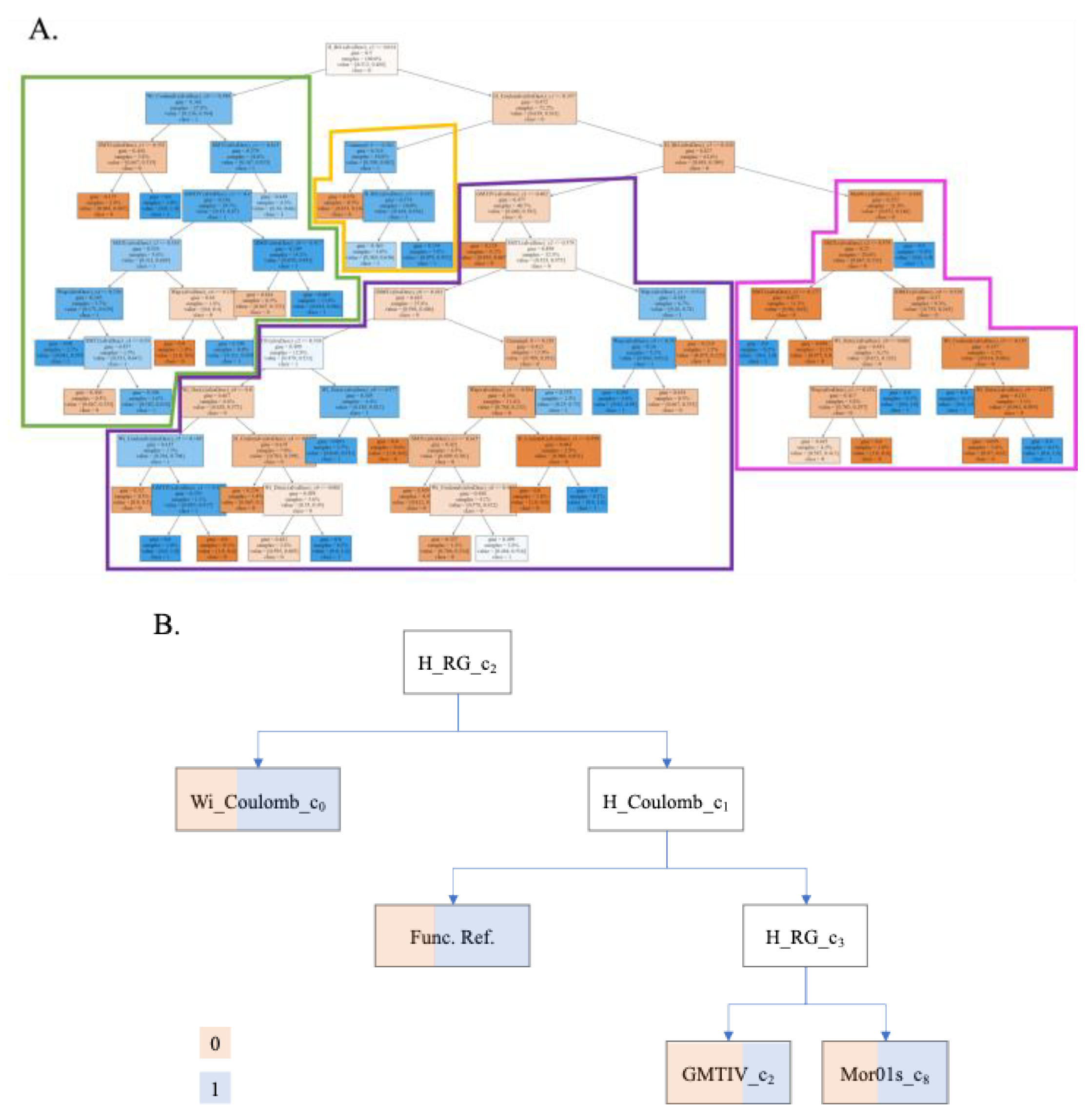
| Input Variables ∆Dk(cj) |
Descriptor Code |
Name | Description | Related Condition (cj) |
Condition name |
Nodes Count |
Ref. |
|---|---|---|---|---|---|---|---|
| ∆Wapi(c4) | Wapi | All-path Wiener index | Counts the number of bonds between pairs of atoms to generate a matrix. Does not take hydrogens into account. | 4 | Nozzle inner diameter | 3 | [85] |
| ∆Wapi(c1) | 1 | Extrusion pressure | 3 | ||||
| ∆WiDzvi(c0) | Wi_Dz(v)i | Wiener-like index from Barysz matrix weighted by van der Waals volume | 0 | Measured property | 1 | [82] | |
| ∆WiDzvi(c9) | 9 | Ethanol content | 4 | ||||
| ∆WiCoulombi (c0) | Wi_Coulombi | Wiener-like index from Coulomb matrix | 0 | Measured property | 2 | [86] | |
| ∆WiCoulombi (c5) | 5 | Layers printed | 2 | ||||
| ∆HRGi (c3) | H_RGi | Harary-like index from reciprocal squared geometrical matrix | It counts the number of bonds of disordered atoms, always taking the shortest path. | 3 | Nozzle | 2 | [80,87] |
| ∆HRGi (c2) | 2 | Extrusion speed | 1 | ||||
| ∆HCoulombi (c1) | H_Coulombi | Harary-like index from Coulomb matrix | 1 | Extrusion pressure | 3 | ||
| ∆HCoulombi (c4) | 4 | Nozzle inner diameter | 1 | ||||
| ∆Mor01si(c3) | Mor01si | Moran autocorrelation of lag 1 weighted by I-state | It is a correlation of two signals between atoms close to each other in space. | 3 | Nozzle | 1 | [88] |
| ∆GMTIVi(c1) | GMTIVi | Gutman Molecular Topological Index by valence vertex degrees | A weighted sum that considers the vertices and valences of all pairs of atoms in a graph. | 1 | Extrusion pressure | 2 | [83,89] |
| ∆GMTIVi(c2) | 2 | 1 | |||||
| ∆SMTIi(c1) | SMTIi | Schultz Molecular Topological Index | 1 | 4 | [74] | ||
| ∆SMTIi(c2) | 2 | 5 | |||||
| ∆IDMTi(c0) | IDMTi | Total information content on the distance magnitude | 0 | Measured property | 2 | ||
| f(vi,j)ref | Reference function | Value dependent on the property to be calculated. | - | 2 |
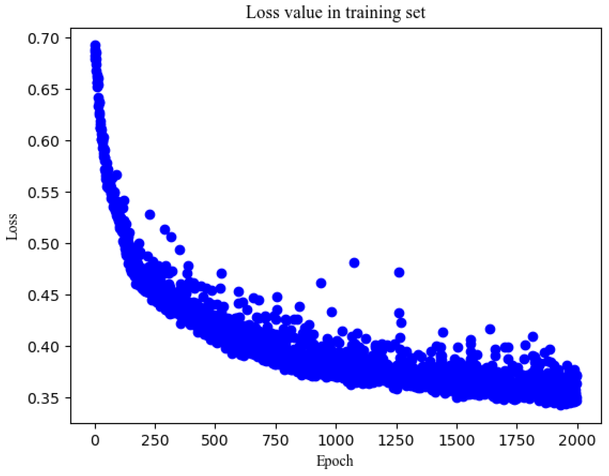
| Epoch | Batch Size |
Train | Test | |||||||
|---|---|---|---|---|---|---|---|---|---|---|
| Sp (%) |
Sn (%) |
Ac (%) |
AUC | Sp (%) |
Sn (%) |
Ac (%) |
AUC | Loss | ||
| 32 | 66.9 | 80.1 | 73.2 | 0.832 | 61.8 | 82.6 | 72.2 | 0.783 | 0.611 | |
| 100 | 64 | 84.8 | 66.7 | 76.2 | 0.807 | 78.8 | 63 | 70.9 | 0.761 | 0.582 |
| 128 | 60.8 | 78.2 | 69.1 | 0.818 | 56.7 | 78.3 | 67.5 | 0.774 | 0.61 | |
| 200 | 32 | 79.4 | 74.6 | 77.1 | 0.861 | 73.7 | 73.6 | 73.7 | 0.792 | 0.596 |
| 64 | 69.8 | 83.4 | 76.3 | 0.858 | 64.0 | 78.3 | 71.1 | 0.788 | 0.614 | |
| 128 | 83.0 | 69.8 | 76.6 | 0.856 | 76.3 | 66.8 | 71.5 | 0.789 | 0.602 | |
| 500 | 32 | 86.6 | 68.6 | 78.3 | 0.895 | 78.4 | 66 | 72.2 | 0.815 | 0.656 |
| 1000 | 32 | 83.5 | 80.7 | 82.1 | 0.906 | 75.0 | 78.7 | 76.8 | 0.830 | 0.659 |
| 2000 | 32 | 79.4 | 81.2 | 80.3 | 0.915 | 72.5 | 80.0 | 76.2 | 0.815 | 0.886 |
| Parameter | Value | Classification Observed |
Classification Predicted |
|
|---|---|---|---|---|
| ChiMA | Uniformity | 0.94 | 1 | 1 |
| Expansion | 6.44 | 0 | 0 | |
| Porosity | 0.38 | 0 | 0 | |
| ChiMA + PEGDA |
Uniformity | 0.98 | 1 | 0 |
| Expansion | 2.78 | 0 | 0 | |
| Porosity | 0.69 | 0 | 0 |
| Extrusion speed (mm/s) (c2) | Property | |||||
| 1 | 7 | 10 | 25 | |||
|
Extrusion P (kPa) (c1) |
25 | 0.071 | 0.927 | 0.071 | 0.148 | Expansion |
| 30 | 0.583 | 0.148 | 0.583 | 0.071 | ||
| 35 | 0.148 | 0.071 | 0.148 | 0.927 | ||
| 48 | 0.071 | 0.927 | 0.071 | 0.148 | ||
| 25 | 0.071 | 0.927 | 0.071 | 0.148 | Pr | |
| 30 | 0.583 | 0.148 | 0.583 | 0.071 | ||
| 35 | 0.148 | 0.071 | 0.148 | 0.927 | ||
| 48 | 0.071 | 0.927 | 0.071 | 0.148 | ||
| 25 | 0.927 | 0.148 | 0.927 | 0.071 | U | |
| 30 | 0.148 | 0.071 | 0.148 | 0.583 | ||
| 35 | 0.071 | 0.927 | 0.071 | 0.148 | ||
| 48 | 0.927 | 0.148 | 0.927 | 0.071 | ||
| 25 | 0.071 | 0.927 | 0.071 | 1.000 | I | |
| 30 | 0.583 | 1.000 | 0.583 | 0.071 | ||
| 35 | 1.000 | 0.071 | 1.000 | 0.927 | ||
| 48 | 0.071 | 0.927 | 0.071 | 1.000 | ||
| Color-scale for probability values | Low | Medium | High | |||
Disclaimer/Publisher’s Note: The statements, opinions and data contained in all publications are solely those of the individual author(s) and contributor(s) and not of MDPI and/or the editor(s). MDPI and/or the editor(s) disclaim responsibility for any injury to people or property resulting from any ideas, methods, instructions or products referred to in the content. |
© 2024 by the authors. Licensee MDPI, Basel, Switzerland. This article is an open access article distributed under the terms and conditions of the Creative Commons Attribution (CC BY) license (http://creativecommons.org/licenses/by/4.0/).


